
Influence of the Characteristics of Weather Information in a Thunderstorm-Related Power Outage Prediction System


Abstract
:1. Introduction
2. Materials and Methods
2.1. Data
2.1.1. Weather
2.1.2. Infrastructure and Outage Data
2.1.3. Environmental Data
2.2. Outage Modeling
2.3. Analysis
3. Results
3.1. Weather Analysis
3.2. The Outage Models
3.2.1. Spatial Skill
3.2.2. Outage Model Variable Importance
4. Discussion
5. Conclusions
Author Contributions
Funding
Institutional Review Board Statement
Informed Consent Statement
Data Availability Statement
Conflicts of Interest
Abbreviations
| NWP | Numerical Weather Prediction |
| WRF | Weather Research and Forecasting model |
| RTMA | Real-Time Mesoscale Analysis |
| RMSLE | Root Mean Squared Logarithmic Error |
| NSE | Nash–Sutcliffe Efficiency |
| MAPE | Mean Absolute Percent Error |
| CRMSE | Centered Root Mean Squared Error |
| FSS | Fraction Skill Score |
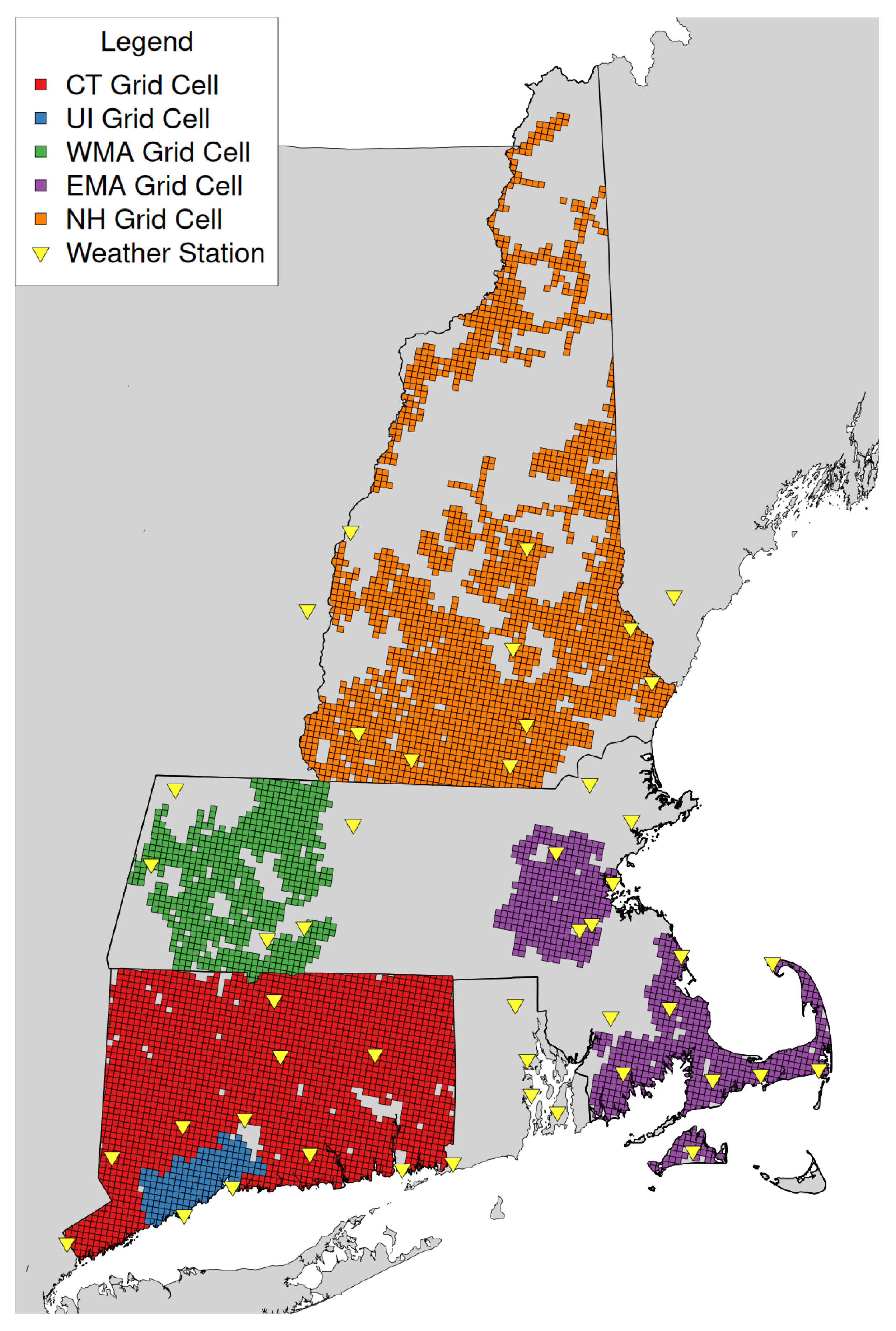
| CT | Eversource Connecticut |
| WMA | Eversource Western Massachusetts |
| EMA | Eversource Eastern Massachusetts |
| NH | Eversource New Hampshire |
| UI | AVANGRID United Illuminating |
| SPI | Standardized Precipitation Index |
| LAI | Leaf Area Index |
| DEM | Digital Elevation Model |
| NLCD | National Land Cover Database |
| 3DEP | 3D Elevation Program |
| GEDI | Global Ecosystem Dynamics Investigation |
| SSURGO | Soil Survey Geographic Database |
| ITSP | Individual Tree Species Parameter |
| WWDT | West Wide Drought Tracker |
| MODIS | Moderate Resolution Imaging Spectroradiometer |
| METAR | Meteorological Aerodrome Reports |
| SPECI | Aviation Selected Special Weather Report |
| NOAA | National Oceanic and Atmospheric Administration |
| NCEP | National Centers for Environmental Prediction |
| USDA | United States Department of Agriculture |
| USGS | United States Geological Survey |
| MRLC | Multi-Resolution Land Characteristics |
Appendix A. Data Features

| Name | Description | Source | Variable Group | RTMA Drp. Loss | WRF Drp. Loss |
|---|---|---|---|---|---|
| ohLength | Length of Overhead Line | Utility Company | Infrastructure | 0.153695 | 0.155182 |
| poleCount | Number of Utility Poles | Utility Company | Infrastructure | 0.152473 | 0.153222 |
| fuseCount | Number of Fuses | Utility Company | Infrastructure | 0.152181 | 0.153253 |
| reclrCount | Number of Reclosers | Utility Company | Infrastructure | 0.152233 | 0.153057 |
| prec11 | Percent NLCD 11—Open Water | NLCD 2016 [51] | Land Cover | 0.151933 | 0.152713 |
| prec21 | Percent NLCD 21—Developed, Open | NLCD 2016 [51] | Land Cover | 0.152056 | 0.152876 |
| prec22 | Percent NLCD 22—Developed, Low | NLCD 2016 [51] | Land Cover | 0.151910 | 0.152749 |
| prec23 | Percent NLCD 23—Developed, Medium | NLCD 2016 [51] | Land Cover | 0.152079 | 0.152963 |
| prec24 | Percent NLCD 24—Developed, High | NLCD 2016 [51] | Land Cover | 0.151989 | 0.152700 |
| prec31 | Percent NLCD 31—Barren | NLCD 2016 [51] | Land Cover | 0.151927 | 0.152714 |
| prec41 | Percent NLCD 41—Deciduous Forest | NLCD 2016 [51] | Land Cover | 0.151974 | 0.152783 |
| prec42 | Percent NLCD 42—Evergreen Forest | NLCD 2016 [51] | Land Cover | 0.151936 | 0.152731 |
| prec43 | Percent NLCD 43—Mixed Forest | NLCD 2016 [51] | Land Cover | 0.151861 | 0.152732 |
| prec52 | Percent NLCD 52—Shrub | NLCD 2016 [51] | Land Cover | 0.151933 | 0.152704 |
| prec71 | Percent NLCD 71—Grassland | NLCD 2016 [51] | Land Cover | 0.151928 | 0.152699 |
| prec82 | Percent NLCD 82—Cultivated Crops | NLCD 2016 [51] | Land Cover | 0.151933 | 0.152715 |
| prec95 | Percent NLCD 95—Herbaceous Wetlands | NLCD 2016 [51] | Land Cover | 0.151934 | 0.152713 |
| avgCanopy | Mean Percent Tree Canopy Cover | NLCD Tree Canopy 2016 [52] | Vegetation | 0.152329 | 0.152956 |
| stdCanopy | Standard Deviation of Canopy Cover | NLCD Tree Canopy 2016 [52] | Vegetation | 0.151968 | 0.152736 |
| avgVegHgt | Mean Vegetation Height | GEDI 2019 [53] | Vegetation | 0.152037 | 0.152906 |
| stdVegHgt | Standard Deviation of Vegetation Height | GEDI 2019 [53] | Vegetation | 0.151945 | 0.152771 |
| avgHardBA | Mean Hardwood Basal Area | ITSP [56] | Vegetation | 0.151903 | 0.152714 |
| stdHardBA | Standard Deviation of Hardwood BA | ITSP [56] | Vegetation | 0.151939 | 0.152722 |
| avgHardSDI | Mean Hardwood Stand Density Index | ITSP [56] | Vegetation | 0.151963 | 0.152686 |
| stdHardSDI | Standard Deviation of Hardwood SDI | ITSP [56] | Vegetation | 0.151919 | 0.152698 |
| avgSoftBA | Mean Softwood Basal Area | ITSP [56] | Vegetation | 0.151914 | 0.152702 |
| stdSoftBA | Standard Deviation of Softwood BA | ITSP [56] | Vegetation | 0.151881 | 0.152691 |
| avgSoftSDI | Mean Softwood Stand Density Index | ITSP [56] | Vegetation | 0.151927 | 0.152677 |
| stdSoftSDI | Standard Deviation of Softwood SDI | ITSP [56] | Vegetation | 0.151891 | 0.152684 |
| avgBA | Mean Total Basal Area | ITSP [56] | Vegetation | 0.151950 | 0.152737 |
| stdBA | Standard Deviation of Total Basal Area | ITSP [56] | Vegetation | 0.151910 | 0.152776 |
| avgSDI | Mean Total Stand Density Index | ITSP [56] | Vegetation | 0.151951 | 0.152698 |
| stdSDI | Standard Deviation of Total SDI | ITSP [56] | Vegetation | 0.151981 | 0.152767 |
| avgDQ | Mean Total Quadratic Mean Diameter | ITSP [56] | Vegetation | 0.151929 | 0.152718 |
| stdDQ | Standard Deviation of Total DQ | ITSP [56] | Vegetation | 0.151936 | 0.152760 |
| avgTF | Mean of Total Frequency | ITSP [56] | Vegetation | 0.152247 | 0.153137 |
| stdTF | Standard Deviation of TF | ITSP [56] | Vegetation | 0.151984 | 0.152783 |
| avgTPA | Mean of Trees per Acre | ITSP [56] | Vegetation | 0.151881 | 0.152653 |
| stdTPA | Standard Deviation of TPA | ITSP [56] | Vegetation | 0.151932 | 0.152690 |
| LAI | Leaf Area Index | MODIS [9,79] | Vegetation | 0.152083 | 0.152848 |
| avgDEM | Mean Elevation | 3DEP [54] | Elevation | 0.151837 | 0.152660 |
| stdDEM | Standard Deviation of Elevation | 3DEP [54] | Elevation | 0.151924 | 0.152720 |
| elvDiff | Difference of avgDEM and weather elevation | 3DEP [54], RTMA [37], WRF [80] | Elevation | 0.151931 | 0.152706 |
| spi1 | One Month Standardized Precipitation Index | WWDT [57] | Drought | 0.151987 | 0.153005 |
| spi3 | Three Month Standardized Precipitation Index | WWDT [57] | Drought | 0.152001 | 0.152830 |
| spi12_0 | 12 Month SPI, current | WWDT [57] | Drought | 0.151998 | 0.152773 |
| spi12_1 | 12 Month SPI, 1 year prior | WWDT [57] | Drought | 0.152137 | 0.152853 |
| spi12_2 | 12 Month SPI, 2 years prior | WWDT [57] | Drought | 0.152075 | 0.152831 |
| spi12_3 | 12 Month SPI, 3 years prior | WWDT [57] | Drought | 0.152155 | 0.152853 |
| spi12_4 | 12 Month SPI, 4 years prior | WWDT [57] | Drought | 0.152027 | 0.152809 |
| spi12_5 | 12 Month SPI, 5 years prior | WWDT [57] | Drought | 0.151939 | 0.152801 |
| hydNo | Percent not hydric soils | SSURGO [55] | Soil Type | 0.151954 | 0.152771 |
| siltTotal | Percent Silt Content | SSURGO [55] | Soil Type | 0.151943 | 0.152747 |
| clayTotal | Percent Clay Content | SSURGO [55] | Soil Type | 0.151929 | 0.152717 |
| rockTotal | Percent of Rock Content | SSURGO [55] | Soil Type | 0.151966 | 0.152738 |
| soilDepth | Depth of Soil | SSURGO [55] | Soil Type | 0.151847 | 0.152661 |
| orgMat | Percent of Organic Material | SSURGO [55] | Soil Type | 0.151949 | 0.152743 |
| soilDens | Soil Density | SSURGO [55] | Soil Type | 0.151950 | 0.152730 |
| kSat | Saturated Hydraulic Conductivity | SSURGO [55] | Soil Type | 0.151945 | 0.152732 |
| satP | Soil Porosity | SSURGO [55] | Soil Type | 0.151961 | 0.152716 |
| avgTMP | Mean Air Temperature | RTMA [37], WRF [80] | Temperature | 0.152191 | 0.152650 |
| stdTMP | Standard Deviation of Air Temp | RTMA [37], WRF [80] | Temperature | 0.152156 | 0.152819 |
| maxTMP | Maximum Air Temperature | RTMA [37], WRF [80] | Temperature | 0.152685 | 0.153235 |
| minTMP | Minimum Air Temperature | RTMA [37], WRF [80] | Temperature | 0.151925 | 0.152873 |
| sumTMP | Sum of Air Temperatures | RTMA [37], WRF [80] | Temperature | 0.152029 | 0.152741 |
| peakTMP | Mean Temp during peak winds | RTMA [37], WRF [80] | Temperature | 0.152020 | 0.152780 |
| avgDPT | Mean Dew Point Temperature | RTMA [37], WRF [80] | Dew Point | 0.151976 | 0.152767 |
| stdDPT | Standard Deviation of Dew Point | RTMA [37], WRF [80] | Dew Point | 0.152013 | 0.152804 |
| maxDPT | Maximum Dew Point Temperature | RTMA [37], WRF [80] | Dew Point | 0.151926 | 0.152687 |
| minDPT | Minimum Dew Point Temperature | RTMA [37], WRF [80] | Dew Point | 0.151941 | 0.152832 |
| sumDPT | Sum of Dew Point Temperatures | RTMA [37], WRF [80] | Dew Point | 0.152012 | 0.152792 |
| peakDPT | Mean Dew Point during peak winds | RTMA [37], WRF [80] | Dew Point | 0.152007 | 0.152723 |
| avgPRES | Mean Surface Pressure | RTMA [37], WRF [80] | Pressure | 0.151914 | 0.152716 |
| stdPRES | Standard Deviation of Pressure | RTMA [37], WRF [80] | Pressure | 0.152297 | 0.152797 |
| maxPRES | Maximum Surface Pressure | RTMA [37], WRF [80] | Pressure | 0.151950 | 0.152735 |
| minPRES | Minimum Surface Pressure | RTMA [37], WRF [80] | Pressure | 0.151946 | 0.152737 |
| sumPRES | Sum of Surface Pressures | RTMA [37], WRF [80] | Pressure | 0.151943 | 0.152706 |
| peakPRES | Mean Pressure during peak winds | RTMA [37], WRF [80] | Pressure | 0.151960 | 0.152694 |
| avgSPFH | Mean Specific Humidity | RTMA [37], WRF [80] | Humidity | 0.152062 | 0.152817 |
| stdSPFH | Standard Deviation of Spec. Humidity | RTMA [37], WRF [80] | Humidity | 0.152018 | 0.152836 |
| maxSPFH | Maximum Specific Humidity | RTMA [37], WRF [80] | Humidity | 0.151949 | 0.152751 |
| minSPFH | Minimum Specific Humidity | RTMA [37], WRF [80] | Humidity | 0.152082 | 0.152905 |
| sumSPFH | Sum of Specific Humidities | RTMA [37], WRF [80] | Humidity | 0.152163 | 0.152752 |
| peakSPFH | Mean of Spec. Humidity during peak winds | RTMA [37], WRF [80] | Humidity | 0.151984 | 0.152767 |
| avgWIND | Mean 10m Wind Speed | RTMA [37], WRF [80] | Wind/Gust | 0.151961 | 0.152710 |
| stdWIND | Standard Deviation of 10m Wind Speed | RTMA [37], WRF [80] | Wind/Gust | 0.151954 | 0.152750 |
| maxWIND | Maximum 10m Wind Speed | RTMA [37], WRF [80] | Wind/Gust | 0.151977 | 0.152748 |
| minWIND | Minimum 10m Wind Speed | RTMA [37], WRF [80] | Wind/Gust | 0.151997 | 0.152745 |
| sumWIND | Sum of Wind Speeds | RTMA [37], WRF [80] | Wind/Gust | 0.151972 | 0.152716 |
| peakWIND | Mean wind speed during peak winds | RTMA [37], WRF [80] | Wind/Gust | 0.151948 | 0.152742 |
| avgGUST | Mean Wind Gust Speed | RTMA [37], WRF [80] | Wind/Gust | 0.152045 | 0.152836 |
| stdGUST | Standard Deviation of Wind Gust Speed | RTMA [37], WRF [80] | Wind/Gust | 0.151985 | 0.152769 |
| maxGUST | Maximum Wind Gust Speed | RTMA [37], WRF [80] | Wind/Gust | 0.152040 | 0.152752 |
| minGUST | Minimum Wind Gust Speed | RTMA [37], WRF [80] | Wind/Gust | 0.152089 | 0.152746 |
| sumGUST | Sum of Wind Gusts | RTMA [37], WRF [80] | Wind/Gust | 0.151988 | 0.152746 |
| peakGUST | Mean Wind Gust Speed during peak winds | RTMA [37], WRF [80] | Wind/Gust | 0.152039 | 0.152748 |
| avgLFSH | Mean Leaf Stress | MODIS [9,79], RTMA [37], WRF [80] | Wind/Gust | 0.151991 | 0.152744 |
| stdLFSH | Standard Deviation of Leaf Stress | MODIS [9,79], RTMA [37], WRF [80] | Wind/Gust | 0.151961 | 0.152738 |
| maxLFSH | Maximum Leaf Stress | MODIS [9,79], RTMA [37], WRF [80] | Wind/Gust | 0.151980 | 0.152743 |
| minLFSH | Minimum Leaf Stress | MODIS [9,79], RTMA [37], WRF [80] | Wind/Gust | 0.151963 | 0.152755 |
| sumLFSH | Sum of Leaf Stresses | MODIS [9,79], RTMA [37], WRF [80] | Wind/Gust | 0.152024 | 0.152760 |
| peakLFSH | Mean Leaf Stress during peak winds | MODIS [9,79], RTMA [37], WRF [80] | Wind/Gust | 0.151961 | 0.152826 |
| wgt5 | Hours of Winds >5 m/s | RTMA [37], WRF [80] | Wind/Gust | 0.151974 | 0.152793 |
| cowgt5 | Continuous Hours of Winds >5 m/s | RTMA [37], WRF [80] | Wind/Gust | 0.151952 | 0.152770 |
| ggt13 | Hours of Gusts >13 m/s | RTMA [37], WRF [80] | Wind/Gust | 0.151967 | 0.152997 |
| ggt17 | Hours of Gusts >17 m/s | RTMA [37], WRF [80] | Wind/Gust | 0.151932 | 0.152729 |
| ggt22 | Hours of Gusts >22 m/s | RTMA [37], WRF [80] | Wind/Gust | 0.151934 | 0.152717 |
| coggt13 | Continuous Hours of Gusts >13 m/s | RTMA [37], WRF [80] | Wind/Gust | 0.151935 | 0.152804 |
| coggt17 | Continuous Hours of Gusts >17 m/s | RTMA [37], WRF [80] | Wind/Gust | 0.151940 | 0.152736 |
| coggt22 | Continuous Hours of Gusts >22 m/s | RTMA [37], WRF [80] | Wind/Gust | 0.151945 | 0.152719 |
| typWDIR | Typical (mean) wind direction of all storms | RTMA [37], WRF [80] | Wind/Gust | 0.152005 | 0.152712 |
| medWDIR | Median Wind direction of storm | RTMA [37], WRF [80] | Wind/Gust | 0.152002 | 0.152806 |
| difWDIR | Difference between typWDIR and medWDIR | RTMA [37], WRF [80] | Wind/Gust | 0.151966 | 0.152745 |
| avgPREC | Mean Hourly Precipitation Rate | Stage IV [38], WRF [80] | Precipitation | 0.152209 | 0.152784 |
| stdPREC | Standard Deviation of Precip. Rate | Stage IV [38], WRF [80] | Precipitation | 0.152403 | 0.152731 |
| maxPREC | Maximum Hourly Precipitation Rate | Stage IV [38], WRF [80] | Precipitation | 0.152844 | 0.152773 |
| sumPREC | Total Precipitation | Stage IV [38], WRF [80] | Precipitation | 0.152187 | 0.152746 |
| peakPREC | Mean Precip. Rate during peak winds | Stage IV [38], WRF [80] | Precipitation | 0.152311 | 0.152726 |
Appendix B. Weather Correlations
| Name | Variable Group | RTMA—METAR R | WRF—METAR R |
|---|---|---|---|
| avgTMP | Temperature | 0.9836 | 0.9129 |
| stdTMP | Temperature | 0.9119 | 0.6448 |
| maxTMP | Temperature | 0.9707 | 0.8686 |
| minTMP | Temperature | 0.9443 | 0.8592 |
| sumTMP | Temperature | 0.9119 | 0.8459 |
| peakTMP | Temperature | 0.7814 | 0.6480 |
| avgDPT | Dew Point | 0.9798 | 0.9461 |
| stdDPT | Dew Point | 0.9092 | 0.7349 |
| maxDPT | Dew Point | 0.9608 | 0.8966 |
| minDPT | Dew Point | 0.9511 | 0.8897 |
| sumDPT | Dew Point | 0.9234 | 0.8921 |
| peakDPT | Dew Point | 0.8348 | 0.7189 |
| avgPRES | Pressure | 0.1700 | 0.1588 |
| stdPRES | Pressure | 0.9766 | 0.9392 |
| maxPRES | Pressure | 0.1498 | 0.1363 |
| minPRES | Pressure | 0.2200 | 0.2038 |
| sumPRES | Pressure | 0.0015 | 0.0013 |
| peakPRES | Pressure | 0.1708 | 0.1469 |
| avgSPFH | Humidity | 0.9735 | 0.9274 |
| stdSPFH | Humidity | 0.8878 | 0.6932 |
| maxSPFH | Humidity | 0.9470 | 0.8648 |
| minSPFH | Humidity | 0.9500 | 0.8799 |
| sumSPFH | Humidity | 0.9204 | 0.8735 |
| peakSPFH | Humidity | 0.8219 | 0.7002 |
| avgWIND | Wind/Gust | 0.6346 | 0.5879 |
| stdWIND | Wind/Gust | 0.3217 | 0.1736 |
| maxWIND | Wind/Gust | 0.3327 | 0.2667 |
| minWIND | Wind/Gust | 0.5053 | 0.3046 |
| sumWIND | Wind/Gust | 0.6057 | 0.5643 |
| peakWIND | Wind/Gust | 0.3632 | 0.3246 |
| avgGUST | Wind/Gust | 0.5915 | 0.5056 |
| stdGUST | Wind/Gust | 0.1411 | 0.0627 |
| maxGUST | Wind/Gust | 0.2484 | 0.1067 |
| minGUST | Wind/Gust | 0.0060 | 0.0091 |
| sumGUST | Wind/Gust | 0.5789 | 0.4957 |
| peakGUST | Wind/Gust | 0.1487 | 0.0625 |
| avgLFSH | Wind/Gust | 0.5512 | 0.5444 |
| stdLFSH | Wind/Gust | 0.3583 | 0.2756 |
| maxLFSH | Wind/Gust | 0.2845 | 0.2249 |
| minLFSH | Wind/Gust | 0.4397 | 0.2735 |
| sumLFSH | Wind/Gust | 0.5382 | 0.5385 |
| peakLFSH | Wind/Gust | 0.2939 | 0.2786 |
| wgt5 | Wind/Gust | 0.4230 | 0.4820 |
| cowgt5 | Wind/Gust | 0.3837 | 0.3517 |
| ggt13 | Wind/Gust | 0.4432 | 0.2149 |
| ggt17 | Wind/Gust | 0.0352 | 0.0137 |
| ggt22 | Wind/Gust | NA 1 | 0.0000 |
| coggt13 | Wind/Gust | 0.4110 | 0.1665 |
| coggt17 | Wind/Gust | 0.0396 | 0.0105 |
| coggt22 | Wind/Gust | NA 1 | 0.0000 |
| typWDIR | Wind/Gust | 0.0054 | 0.1378 |
| medWDIR | Wind/Gust | 0.3357 | 0.0304 |
| difWDIR | Wind/Gust | 0.2362 | 0.0219 |
| avgPREC | Precipitation | 0.6056 | 0.0886 |
| stdPREC | Precipitation | 0.5589 | 0.0622 |
| maxPREC | Precipitation | 0.5298 | 0.0538 |
| sumPREC | Precipitation | 0.5585 | 0.0862 |
| peakPREC | Precipitation | 0.1989 | 0.0279 |
Appendix C. Error Metrics
References
- Economic Benefits of Increasing Electric Grid Resilience to Weather Outages; Technical Report; Executive Office of the President: Washington, DC, USA, 2013.
- Lubkeman, D.; Julian, D. Large scale storm outage management. In Proceedings of the IEEE Power Engineering Society General Meeting, Denver, CO, USA, 6–10 June 2004; Volume 2, pp. 16–22. [Google Scholar] [CrossRef]
- Hall, K.L. Out of Sight, Out of Mind; Technical Report; Edison Electric Institute: Washington, DC, USA, 2012. [Google Scholar]
- Mukherjee, S.; Nateghi, R.; Hastak, M. A multi-hazard approach to assess severe weather-induced major power outage risks in the U.S. Reliab. Eng. Syst. Saf. 2018, 175, 283–305. [Google Scholar] [CrossRef]
- Sander, J.; Eichner, J.F.; Faust, E.; Steuer, M. Rising Variability in Thunderstorm-Related U.S. Losses as a Reflection of Changes in Large-Scale Thunderstorm Forcing. Weather. Clim. Soc. 2013, 5, 317–331. [Google Scholar] [CrossRef] [Green Version]
- Diffenbaugh, N.S.; Scherer, M.; Trapp, R.J. Robust increases in severe thunderstorm environments in response to greenhouse forcing. Proc. Natl. Acad. Sci. USA 2013, 110, 16361–16366. [Google Scholar] [CrossRef] [Green Version]
- Scaff, L.; Prein, A.F.; Li, Y.; Liu, C.; Rasmussen, R.; Ikeda, K. Simulating the convective precipitation diurnal cycle in North America’s current and future climate. Clim. Dyn. 2020, 55, 369–382. [Google Scholar] [CrossRef]
- Li, Z.; Singhee, A.; Wang, H.; Raman, A.; Siegel, S.; Heng, F.L.; Mueller, R.; Labut, G. Spatio-temporal forecasting of weather-driven damage in a distribution system. In Proceedings of the 2015 IEEE Power & Energy Society General Meeting, Denver, CO, USA, 26–30 July 2015; pp. 1–5. [Google Scholar] [CrossRef]
- Cerrai, D.; Wanik, D.W.; Bhuiyan, M.A.E.; Zhang, X.; Yang, J.; Frediani, M.E.B.; Anagnostou, E.N. Predicting Storm Outages Through New Representations of Weather and Vegetation. IEEE Access 2019, 7, 29639–29654. [Google Scholar] [CrossRef]
- Wanik, D.W.; Anagnostou, E.N.; Hartman, B.M.; Frediani, M.E.B.; Astitha, M. Storm outage modeling for an electric distribution network in Northeastern USA. Nat. Hazards 2015, 79, 1359–1384. [Google Scholar] [CrossRef]
- Kankanala, P.; Das, S.; Pahwa, A. AdaBoost+: An Ensemble Learning Approach for Estimating Weather-Related Outages in Distribution Systems. IEEE Trans. Power Syst. 2014, 29, 359–367. [Google Scholar] [CrossRef] [Green Version]
- Han, S.R.; Guikema, S.D.; Quiring, S.M.; Lee, K.H.; Rosowsky, D.; Davidson, R.A. Estimating the spatial distribution of power outages during hurricanes in the Gulf coast region. Reliab. Eng. Syst. Saf. 2009, 94, 199–210. [Google Scholar] [CrossRef]
- Quiring, S.M.; Zhu, L.; Guikema, S.D. Importance of soil and elevation characteristics for modeling hurricane-induced power outages. Nat. Hazards 2011, 58, 365–390. [Google Scholar] [CrossRef]
- Guikema, S.D.; Nateghi, R.; Quiring, S.M.; Staid, A.; Reilly, A.C.; Gao, M. Predicting Hurricane Power Outages to Support Storm Response Planning. IEEE Access 2014, 2, 1364–1373. [Google Scholar] [CrossRef]
- McRoberts, D.B.; Quiring, S.M.; Guikema, S.D. Improving Hurricane Power Outage Prediction Models Through the Inclusion of Local Environmental Factors. Risk Anal. 2018, 38, 2722–2737. [Google Scholar] [CrossRef]
- D’Amico, D.F.; Quiring, S.M.; Maderia, C.M.; McRoberts, D.B. Improving the Hurricane Outage Prediction Model by including tree species. Clim. Risk Manag. 2019, 25, 100193. [Google Scholar] [CrossRef]
- Yang, F.; Watson, P.; Koukoula, M.; Anagnostou, E.N. Enhancing Weather-Related Power Outage Prediction by Event Severity Classification. IEEE Access 2020, 8, 60029–60042. [Google Scholar] [CrossRef]
- Watson, P.L.; Cerrai, D.; Koukoula, M.; Wanik, D.W.; Anagnostou, E. Weather-related power outage model with a growing domain: Structure, performance, and generalisability. J. Eng. 2020, 2020, 817–826. [Google Scholar] [CrossRef]
- Tervo, R.; Láng, I.; Jung, A.; Mäkelä, A. Predicting power outages caused by extratropical storms. Nat. Hazards Earth Syst. Sci. 2021, 21, 607–627. [Google Scholar] [CrossRef]
- Singhee, A.; Wang, H. Probabilistic forecasts of service outage counts from severe weather in a distribution grid. In Proceedings of the 2017 IEEE Power & Energy Society General Meeting, Chicago, IL, USA, 16–20 July 2017; pp. 1–5. [Google Scholar] [CrossRef]
- Yue, M.; Toto, T.; Jensen, M.P.; Giangrande, S.E.; Lofaro, R. A Bayesian Approach-Based Outage Prediction in Electric Utility Systems Using Radar Measurement Data. IEEE Trans. Smart Grid 2018, 9, 6149–6159. [Google Scholar] [CrossRef]
- Zhou, Y.; Pahwa, A.; Yang, S.S. Modeling Weather-Related Failures of Overhead Distribution Lines. IEEE Trans. Power Syst. 2006, 21, 1683–1690. [Google Scholar] [CrossRef]
- Kankanala, P.; Pahwa, A.; Das, S. Regression models for outages due to wind and lightning on overhead distribution feeders. In Proceedings of the 2011 IEEE Power and Energy Society General Meeting, San Detroit, MI, USA, 24–28 July 2011; pp. 1–4. [Google Scholar] [CrossRef]
- Hohenegger, C.; Schar, C. Atmospheric Predictability at Synoptic Versus Cloud-Resolving Scales. Bull. Am. Meteorol. Soc. 2007, 88, 1783–1794. [Google Scholar] [CrossRef]
- Sun, J.; Xue, M.; Wilson, J.W.; Zawadzki, I.; Ballard, S.P.; Onvlee-Hooimeyer, J.; Joe, P.; Barker, D.M.; Li, P.W.; Golding, B.; et al. Use of NWP for Nowcasting Convective Precipitation: Recent Progress and Challenges. Bull. Am. Meteorol. Soc. 2014, 95, 409–426. [Google Scholar] [CrossRef] [Green Version]
- Yano, J.I.; Ziemiański, M.Z.; Cullen, M.; Termonia, P.; Onvlee, J.; Bengtsson, L.; Carrassi, A.; Davy, R.; Deluca, A.; Gray, S.L.; et al. Scientific Challenges of Convective-Scale Numerical Weather Prediction. Bull. Am. Meteorol. Soc. 2018, 99, 699–710. [Google Scholar] [CrossRef]
- Papadopoulos, A.; Chronis, T.G.; Anagnostou, E.N. Improving Convective Precipitation Forecasting through Assimilation of Regional Lightning Measurements in a Mesoscale Model. Mon. Weather Rev. 2005, 133, 1961–1977. [Google Scholar] [CrossRef] [Green Version]
- Hu, M.; Xue, M. Impact of Configurations of Rapid Intermittent Assimilation of WSR-88D Radar Data for the 8 May 2003 Oklahoma City Tornadic Thunderstorm Case. Mon. Weather Rev. 2007, 135, 507–525. [Google Scholar] [CrossRef] [Green Version]
- Benjamin, S.G.; Weygandt, S.S.; Brown, J.M.; Hu, M.; Alexander, C.R.; Smirnova, T.G.; Olson, J.B.; James, E.P.; Dowell, D.C.; Grell, G.A.; et al. A North American Hourly Assimilation and Model Forecast Cycle: The Rapid Refresh. Mon. Weather Rev. 2016, 144, 1669–1694. [Google Scholar] [CrossRef]
- Clark, A.J.; Gallus, W.A.; Xue, M.; Kong, F. A Comparison of Precipitation Forecast Skill between Small Convection-Allowing and Large Convection-Parameterizing Ensembles. Weather Forecast. 2009, 24, 1121–1140. [Google Scholar] [CrossRef] [Green Version]
- Roberts, B.; Gallo, B.T.; Jirak, I.L.; Clark, A.J. The High Resolution Ensemble Forecast (HREF) system: Applications and Performance for Forecasting Convective Storms. Meteorology 2019. [Google Scholar] [CrossRef] [Green Version]
- Bouttier, F.; Marchal, H. Probabilistic thunderstorm forecasting by blending multiple ensembles. Tellus A Dyn. Meteorol. Oceanogr. 2020, 72, 1–19. [Google Scholar] [CrossRef] [Green Version]
- Alpay, B.A.; Wanik, D.; Watson, P.; Cerrai, D.; Liang, G.; Anagnostou, E. Dynamic Modeling of Power Outages Caused by Thunderstorms. Forecasting 2020, 2, 151–162. [Google Scholar] [CrossRef]
- Sheild, S.A.; Quiring, S.M.; McRoberts, D.B. Development of a Thunderstorm Outage Prediction Model. Ph.D. Thesis, The Ohio State University, Columbus, OH, USA, 2018. [Google Scholar]
- Kabir, E.; Guikema, S.D.; Quiring, S.M. Predicting Thunderstorm-Induced Power Outages to Support Utility Restoration. IEEE Trans. Power Syst. 2019, 34, 4370–4381. [Google Scholar] [CrossRef]
- Babbage, C. Passages from the Life of a Philosopher; Longman, Green, Longman, Roberts, & Green: London, UK, 1864. [Google Scholar]
- De Pondeca, M.S.F.V.; Manikin, G.S.; DiMego, G.; Benjamin, S.G.; Parrish, D.F.; Purser, R.J.; Wu, W.S.; Horel, J.D.; Myrick, D.T.; Lin, Y.; et al. The Real-Time Mesoscale Analysis at NOAA’s National Centers for Environmental Prediction: Current Status and Development. Weather Forecast. 2011, 26, 593–612. [Google Scholar] [CrossRef]
- Nelson, B.R.; Prat, O.P.; Seo, D.J.; Habib, E. Assessment and Implications of NCEP Stage IV Quantitative Precipitation Estimates for Product Intercomparisons. Weather Forecast. 2016, 31, 371–394. [Google Scholar] [CrossRef]
- NOAA/NWS. RTMA: Real-Time Mesoscale Analysis Data; NOAA/NWS: Washington, DC, USA, 2015.
- Hudlow, M.D. Technological Developments in Real-Time Operational Hydrologic Forecasting in the United States. J. Hydrol. 1988, 102, 69–92. [Google Scholar] [CrossRef]
- Environmental Modeling Center; National Centers for Environmental Prediction; National Weather Service; NOAA; U.S. Department of Commerce. NCEP North American Mesoscale (NAM) 12 km Analysis; U.S. Department of Commerce: Washington, DC, USA, 2015.
- Morrison, H.; Thompson, G.; Tatarskii, V. Impact of Cloud Microphysics on the Development of Trailing Stratiform Precipitation in a Simulated Squall Line: Comparison of One- and Two-Moment Schemes. Mon. Weather Rev. 2009, 137, 991–1007. [Google Scholar] [CrossRef] [Green Version]
- Mlawer, E.J.; Taubman, S.J.; Brown, P.D.; Iacono, M.J.; Clough, S.A. Radiative transfer for inhomogeneous atmospheres: RRTM, a validated correlated-k model for the longwave. J. Geophys. Res. Atmos. 1997, 102, 16663–16682. [Google Scholar] [CrossRef] [Green Version]
- Chou, M.; Suarez, M. An Efficient Thermal Infrared Radiation Parameterization for Use in General Circulations Models. NASA Tech. Memo. 1994, 3, 1–85. [Google Scholar]
- Jiménez, P.A.; Dudhia, J.; González-Rouco, J.F.; Navarro, J.; Montávez, J.P.; García-Bustamante, E. A Revised Scheme for the WRF Surface Layer Formulation. Mon. Weather Rev. 2012, 140, 898–918. [Google Scholar] [CrossRef] [Green Version]
- Tewari, M.; Chen, F.; Wang, W.; Dudhia, J.; LeMone, M.; Mitchell, K.; Ek, M.; Gayno, G.; Wegiel, J.; Cuenca, R. Implementation and verification of the unified NOAH land surface model in the WRF model. In Proceedings of the 20th Conference on Weather Analysis and Forecasting/16th Conference on Numerical Weather Prediction, Seattle, WA, USA, 11–15 January 2004; Volume 1115, pp. 2165–2170. [Google Scholar]
- Hong, S.; Noh, Y.; Dudhia, J. A New Vertical Diffusion Package with an Explicit Treatment of Entrainment Processes. Mon. Weather Rev. 2006, 134, 2318–2341. [Google Scholar] [CrossRef] [Green Version]
- Agostinelli, C.; Lund, U. R Package Circular: Circular Statistics (Version 0.4-93); Department of Environmental Sciences, Informatics and Statistics, Ca’ Foscari University: Venice, Italy; UL: Department of Statistics, California Polytechnic State University: San Luis Obispo, CA, USA, 2017; Available online: https://cran.r-project.org/web/packages/circular/circular.pdf (accessed on 2 February 2021).
- Bivand, R.; Keitt, T.; Rowlingson, B. rgdal: Bindings for the ’Geospatial’ Data Abstraction Library. R Package Version 1.5-23. 2021. Available online: https://cran.r-project.org/web/packages/rgdal/index.html (accessed on 2 February 2021).
- Bivand, R.; Rundel, C. rgeos: Interface to Geometry Engine—Open Source (’GEOS’). R Package Version 0.5-5. 2020. Available online: https://cran.r-project.org/web/packages/rgeos/index.html (accessed on 1 June 2020).
- Jin, S.; Homer, C.; Yang, L.; Danielson, P.; Dewitz, J.; Li, C.; Zhu, Z.; Xian, G.; Howard, D. Overall Methodology Design for the United States National Land Cover Database 2016 Products. Remote Sens. 2019, 11, 2971. [Google Scholar] [CrossRef] [Green Version]
- Coulston, J.W.; Moisen, G.G.; Wilson, B.T.; Finco, M.V.; Cohen, W.B.; Brewer, C.K. Modeling Percent Tree Canopy Cover: A Pilot Study. Photogramm. Eng. Remote Sens. 2012, 78, 715–727. [Google Scholar] [CrossRef] [Green Version]
- Potapov, P.; Li, X.; Hernandez-Serna, A.; Tyukavina, A.; Hansen, M.C.; Kommareddy, A.; Pickens, A.; Turubanova, S.; Tang, H.; Silva, C.E.; et al. Mapping global forest canopy height through integration of GEDI and Landsat data. Remote Sens. Environ. 2021, 253, 112165. [Google Scholar] [CrossRef]
- Gesch, D.; Evans, G.; Oimoen, M.; Arundel, S. The National Elevation Dataset; American Society for Photogrammetry and Remote Sensing: Bethseda, MD, USA, 2018; pp. 83–110. [Google Scholar]
- Soil Survey Staff, Natural Resources Conservation Service. Soil Survey Geographic (SSURGO) Database. 2010. Available online: https://websoilsurvey.nrcs.usda.gov/ (accessed on 21 August 2020).
- Individual Tree Species Parameter Maps. 2015. Available online: https://www.fs.fed.us/foresthealth/applied-sciences/mappingreporting/indiv-tree-parameter-maps.shtml (accessed on 19 March 2021).
- Abatzoglou, J.T.; McEvoy, D.J.; Redmond, K.T. The West Wide Drought Tracker: Drought Monitoring at Fine Spatial Scales. Bull. Am. Meteorol. Soc. 2017, 98, 1815–1820. [Google Scholar] [CrossRef]
- R Core Team. R: A Language and Environment for Statistical Computing; R Foundation for Statistical Computing: Vienna, Austria, 2021. [Google Scholar]
- Kursa, M.B.; Jankowski, A.; Rudnicki, W.R. Boruta—A System for Feature Selection. Fundam. Inform. 2010, 101, 271–285. [Google Scholar] [CrossRef]
- Kursa, M.B.; Rudnicki, W.R. Feature Selection with the Boruta Package. J. Stat. Softw. 2010, 36, 1–13. [Google Scholar] [CrossRef] [Green Version]
- Chipman, H.A.; George, E.I.; McCulloch, R.E. BART: Bayesian additive regression trees. Ann. Appl. Stat. 2010, 4, 266–298. [Google Scholar] [CrossRef]
- Sparapani, R.; Spanbauer, C.; McCulloch, R. Nonparametric Machine Learning and Efficient Computation with Bayesian Additive Regression Trees: The BART R Package. J. Stat. Softw. 2021, 97, 1–66. [Google Scholar] [CrossRef]
- Ardia, D.; Boudt, K.; Carl, P.; Mullen, K.M.; Peterson, B.G. Differential Evolution with DEoptim: An Application to Non-Convex Portfolio Optimization. R J. 2011, 3, 27–34. [Google Scholar] [CrossRef] [Green Version]
- Mullen, K.; Ardia, D.; Gil, D.; Windover, D.; Cline, J. DEoptim: An R Package for Global Optimization by Differential Evolution. J. Stat. Softw. 2011, 40, 1–26. [Google Scholar] [CrossRef] [Green Version]
- National Centers for Environmental Information. Integrated Surface Data (ISD) Archive. Available online: https://www.ncei.noaa.gov/data/global-hourly/access/ (accessed on 3 March 2021).
- Nash, J.; Sutcliffe, J. River flow forecasting through conceptual models part I—A discussion of principles. J. Hydrol. 1970, 10, 282–290. [Google Scholar] [CrossRef]
- Roberts, N.M.; Lean, H.W. Scale-Selective Verification of Rainfall Accumulations from High-Resolution Forecasts of Convective Events. Mon. Weather Rev. 2008, 136, 78–97. [Google Scholar] [CrossRef]
- Gilleland, E.; Ahijevych, D.A.; Brown, B.G.; Ebert, E.E. Verifying Forecasts Spatially. Bull. Am. Meteorol. Soc. 2010, 91, 1365–1376. [Google Scholar] [CrossRef] [Green Version]
- Mittermaier, M.; Roberts, N. Intercomparison of Spatial Forecast Verification Methods: Identifying Skillful Spatial Scales Using the Fractions Skill Score. Weather Forecast. 2010, 25, 343–354. [Google Scholar] [CrossRef]
- Laboratory, N.R.A. Verification: Weather Forecast Verification Utilities. R Package Version 1.42. 2015. Available online: https://CRAN.R-project.org/package=verification.
- Gilleland, E. SpatialVx: Spatial Forecast Verification. R Package Version 0.8. 2021. Available online: https://CRAN.R-project.org/package=SpatialVx (accessed on 3 March 2021).
- Fisher, A.; Rudin, C.; Dominici, F. All Models are Wrong, but Many are Useful: Learning a Variable’s Importance by Studying an Entire Class of Prediction Models Simultaneously. J. Mach. Learn. Res. 2019, 20, 1–81. [Google Scholar]
- Biecek, P. DALEX: Explainers for Complex Predictive Models in R. J. Mach. Learn. Res. 2018, 19, 1–5. [Google Scholar]
- Lee, T.R.; Buban, M.; Turner, D.D.; Meyers, T.P.; Baker, C.B. Evaluation of the High-Resolution Rapid Refresh (HRRR) Model Using Near-Surface Meteorological and Flux Observations from Northern Alabama. Weather Forecast. 2019, 34, 635–663. [Google Scholar] [CrossRef]
- Pichugina, Y.L.; Banta, R.M.; Bonin, T.; Brewer, W.A.; Choukulkar, A.; McCarty, B.J.; Baidar, S.; Draxl, C.; Fernando, H.J.S.; Kenyon, J.; et al. Spatial Variability of Winds and HRRR–NCEP Model Error Statistics at Three Doppler-Lidar Sites in the Wind-Energy Generation Region of the Columbia River Basin. J. Appl. Meteorol. Climatol. 2019, 58, 1633–1656. [Google Scholar] [CrossRef]
- Shucksmith, P.E.; Sutherland-Stacey, L.; Austin, G.L. The spatial and temporal sampling errors inherent in low resolution radar estimates of rainfall: Spatial and temporal sampling errors in low resolution radar estimates of rainfall. Meteorol. Appl. 2011, 18, 354–360. [Google Scholar] [CrossRef]
- Moreau, E.; Testud, J.; Le Bouar, E. Rainfall spatial variability observed by X-band weather radar and its implication for the accuracy of rainfall estimates. Adv. Water Resour. 2009, 32, 1011–1019. [Google Scholar] [CrossRef] [Green Version]
- Zhou, L.; Lin, S.J.; Chen, J.H.; Harris, L.M.; Chen, X.; Rees, S.L. Toward Convective-Scale Prediction within the Next Generation Global Prediction System. Bull. Am. Meteorol. Soc. 2019, 100, 1225–1243. [Google Scholar] [CrossRef]
- Leaf Area Index (1 Month—Terra/MODIS). 2017. Available online: https://modis.gsfc.nasa.gov/data/dataprod/mod15.php (accessed on 17 December 2020).
- Community, WRF. Weather Research and Forecasting (WRF) Model; UCAR/NCAR: Boulder, CO, USA, 2000. [Google Scholar] [CrossRef]


| CT | WMA | EMA | NH | UI | Total | |
|---|---|---|---|---|---|---|
| Number of Storms | 74 | 82 | 69 | 91 | 56 | 372 |
| Territory Grid Cells | 2019 | 638 | 820 | 2128 | 169 | 5774 |
| Total Entries | 149,406 | 52,316 | 56,580 | 193,648 | 9464 | 461,414 |
| Horizontal Resolution | 2 km | |
| Vertical Levels | 51 | |
| Horizontal Grid Scheme | Arakawa C Grid | |
| Nesting | One 6km Nested Domain | |
| Microphysics Option | Thompson Graupel Scheme [42] | |
| Longwave Radiation Option | RRTM Scheme [43] | |
| Shortwave Radiation Option | Goddard Shortwave Scheme [44] | |
| Surface-Layer Option | Revised MM5 Scheme [45] | |
| Land-Surface Option | Noah Land-Surface Model [46] | |
| Planetary Boundary Layer | Yonsei Scheme [47] |
| MdAPE | MAPE | CRMSE | R | NSE | |
|---|---|---|---|---|---|
| RTMA | 31% | 46% | 50 | 0.39 | 0.37 |
| WRF | 35% | 50% | 51 | 0.36 | 0.35 |
Publisher’s Note: MDPI stays neutral with regard to jurisdictional claims in published maps and institutional affiliations. |
© 2021 by the authors. Licensee MDPI, Basel, Switzerland. This article is an open access article distributed under the terms and conditions of the Creative Commons Attribution (CC BY) license (https://creativecommons.org/licenses/by/4.0/).
Share and Cite
Watson, P.L.; Koukoula, M.; Anagnostou, E. Influence of the Characteristics of Weather Information in a Thunderstorm-Related Power Outage Prediction System. Forecasting 2021, 3, 541-560. https://0-doi-org.brum.beds.ac.uk/10.3390/forecast3030034
Watson PL, Koukoula M, Anagnostou E. Influence of the Characteristics of Weather Information in a Thunderstorm-Related Power Outage Prediction System. Forecasting. 2021; 3(3):541-560. https://0-doi-org.brum.beds.ac.uk/10.3390/forecast3030034
Chicago/Turabian StyleWatson, Peter L., Marika Koukoula, and Emmanouil Anagnostou. 2021. "Influence of the Characteristics of Weather Information in a Thunderstorm-Related Power Outage Prediction System" Forecasting 3, no. 3: 541-560. https://0-doi-org.brum.beds.ac.uk/10.3390/forecast3030034