
Probabilistic Day-Ahead Wholesale Price Forecast: A Case Study in Great Britain

1
Energy Systems Catapult, Cannon House, Birmingham B4 6BS, UK
2
Mathematical Institute, University of Oxford, Oxford OX2 6GG, UK
*
Author to whom correspondence should be addressed.
Forecasting 2021, 3(3), 596-632; https://0-doi-org.brum.beds.ac.uk/10.3390/forecast3030038
Submission received: 29 June 2021
/
Revised: 12 August 2021
/
Accepted: 25 August 2021
/
Published: 28 August 2021
(This article belongs to the Special Issue Forecasting Prices in Power Markets)
Abstract
:The energy sector is moving towards a low-carbon, decentralised, and smarter network. The increased uptake of distributed renewable energy and cheaper storage devices provide opportunities for new local energy markets. These local energy markets will require probabilistic price forecasting models to better describe the future price uncertainty. This article considers the application of probabilistic electricity price forecasting models to the wholesale market of Great Britain (GB) and compares them to better understand their capabilities and limits. One of the models that this paper considers is a recent novel X-model that predicts the full supply and demand curves from the bid-stack. The advantage of this model is that it better captures price spikes in the data. In this paper, we provide an adjustment to the model to handle data from GB. In addition to this, we then consider and compare two time-series approaches and a simple benchmark. We compare both point forecasts and probabilistic forecasts on real wholesale price data from GB and consider both point and probabilistic measures.
1. Introduction
Since the liberalisation of the electricity market, forecasting electricity prices has been an important factor in decision making for energy suppliers and generators. Day-ahead wholesale electricity price forecasts are an essential component of the electricity market. In the wholesale market, electricity is traded between suppliers and generators by placing offers and bids, respectively, for different volumes of electricity. This is used to set the wholesale price at which day-ahead electricity is purchased. Energy suppliers generally hedge (purchase ahead) their best forecast of volumes and refine their positions closer to delivery, such as in the day-ahead market. The overall cost of wholesale energy is combined with other cost elements in the tariffs offered to consumers. The wholesale electricity price forecasts are a fundamental input for an energy company’s decision making. Prices are relatively volatile, and hence, probabilistic forecasts are more useful, as they describe the uncertainty associated with different events. In this article, three day-ahead probabilistic electricity price forecasts are developed and tested for Great Britain’s day-ahead wholesale electricity market. One of the focuses will be on a recent method developed in [1] called the X-model, whose focus is on the prediction of spikes in the electricity price.
Until recently, wholesale price forecasting was typically focused on point forecasts. However, in the last few years, probabilistic price forecasting has been gaining interest. The comprehensive 2014 review by Weron [2] showed that very few papers at the time considered probabilistic forecasts. The 2018 review update by Nowotarski and Weron [3], however, highlighted the importance of probabilistic forecasts due to the introduction of the so-called smart grid and the increased uncertainty in supply and demand. A more recent review [4] published after the development presented in this article underlines the need for a rigorous approach and sensible benchmarking in the electricity price forecasting field.
The 2018 review showed that there was an increase in probabilistic electricity price forecasting papers, but the literature is relatively sparse, especially compared to load forecasting, with only 38 papers on probabilistic electricity price forecasting for the period of 2002–2016. There has not been a dramatic change in the number of probabilistic electricity price forecasting papers since the review by Nowotarski and Weron [3]. Using the same search terms as the authors (Scopus query used to find probabilistic electricity price forecasting publications: (TITLE((“probabilistic” AND “forecasting”) OR interval OR density) OR TITLE-ABS-KEY(“probabilistic forecast*” OR “interval forecast*” OR “density forecast*” OR “prediction interval*”)) AND (TITLE (((((“electric*” OR “energy market” OR “power price” OR “power market” OR “power system” OR pool OR “market clearing” OR “energy clearing”) AND (price OR prices OR pricing)) OR lmp OR “locational marginal price”) AND (forecast OR forecasts OR forecasting OR prediction OR predicting OR predictability OR “predictive densit*”)) OR (“price forecasting” AND “smartgrid*”)) OR TITLE-ABS (“electricity price forecasting” OR “forecasting electricity price” OR “day-ahead price forecasting” OR “day-ahead mar*price forecasting” OR (gefcom2014 AND price) OR ((“electricity market” OR “electric energy market”) AND “priceforecasting”) OR (“electricity price” AND (“prediction interval”OR“interval forecast”OR“density forecast” OR “probabilisticforecast”))) AND NOT TITLE (“unit commitment”)) AND (EXCLUDE (AU-ID, “[No Author ID found]” undefined))), we found 11 papers in 2018, 10 in 2019, 16 in 2020, and 8 in 2021 so far. So there has only been a small uptick in probabilistic price forecasting, and much more work in this area is still required. In particular, there was only one paper found on probabilistic price forecasting within the day-ahead wholesale market in Great Britain [5]. In this paper, Maciejowska et al. produced prediction intervals by applying a quantile regression with several individual point forecast methods used as independent variables and the spot price as the dependent variable. The presented method also updated this model by using a PCA to extract common factors, which were used as independent inputs within a quantile regression. A limitation to this work is that they only considered prediction intervals and, hence, did not produce a detailed description of the uncertainty. In addition, they did not consider price spikes.
As summarized in the review by Nowotarski and Weron [3], probabilistic forecasts in the electricity price sector started to appear after 2002 and gained momentum thanks to the Global Energy Forecasting Competition of 2014. Such models can be characterized by the family of the modelling technique used (neural network, traditional statistical time series, hybrid, or other) and the method used to compute the prediction interval. The prediction interval can be computed from historical simulations (also called empirical or sample prediction intervals), from distribution-based forecasts (usually approximating the error distribution with a Gaussian distribution), from bootstrapping, or from quantile regression averaging. The bootstrapping method [6] is particularly popular for neural network methods, but is also used in statistical time-series approaches [7]. The quantile regression averaging method (QRA) proposed by Nowotarski and Weron [8] has gained popularity in the probabilistic electricity price forecasting field and was used by the top two winning teams of the Global Energy Forecasting Competition of 2014 [9,10]. More recently, Uniejewski et al. [11] presented a regularised form of QRA that utilises the LASSO method. A regularised approach was also considered by Banitalebi et al. [12], but while using a triple seasonal exponential smoothing model.
As the probabilistic electricity price forecasting field has developed, statistical time-series approaches have seemed to become proportionally more popular than in the electricity price point forecasting landscape, but neural network approaches—in particular, deep learning—have gained interest in the last few years. He et al. [13] considered deep convolutional neural networks. Brusaferri et al. [14] present a Bayesian deep learning approach to probabilistic day-ahead price forecasts and demonstrated it on both the Italian and Belgian markets.
Statistical time-series approaches, such as linear autoregressive methods and ARIMA models, are common in price forecasting, and have continued to be developed. Recent developments from Marcjasz et al. [15] showed that a nonlinear version of an ARX could outperform its linear counterparts. Uniejewski et al. [16] considered a new class of probabilistic models called seasonal component autoregressive models (SCARX). Since their successful application within the Global Energy Forecasting competition in 2014 [10], generalised additive models have become more popular and have been applied extensively in load and price forecasting. Bernardi and Lisi [17] use a generalised additive model to generate point and prediction intervals and applied it to the Italian electricity market.
There are also some newer and more unique approaches emerging, as well as models that are perhaps common in areas such as load forecasting, but have not been applied as much in price forecasting. Gaussian processes are common in load forecasting. Mehmood et al. [18] used a Gaussian process regression for interval forecasting of SPOT prices. An interesting paper by Taylor [19] considered the generation of prediction intervals by using a quantile approach versus using the less common “expectile” approach. Finally, a unique approach was applied by Kath and Ziel [20], who considered a conformal prediction approach in order to estimate prediction intervals. CP is a framework that considers a non-conformity score on an out-of-sample dataset, and then a threshold is calculated for the one-step-ahead forecast to produce the prediction intervals.
Of particular importance is accurately forecasting price spikes, which are large deviations from the mean price that are either big or small. As discussed in [1], many researchers have considered regime-switching models or jump-diffusion models to predict extreme values, and these do not typically forecast the entire series. The authors of [3] mentioned a few forecasting studies that were designed to estimate spikes; for example, [21] considered an autoregressive conditional hazard model, Ref. [22] used a specific error metric to train and select models while accounting for spikes, and the authors of [23] used a threshold forecasting model. However, there is still unexploited potential in terms of investigating the underlying mechanisms behind price spikes. As pointed out in [1], many studies only model the individual spike and not the entire price time series, and all of them ignore the underlying mechanism that generates the prices. Accounting for some of these drawbacks, Ziel and Steinert developed the so-called X-model, a unique approach that forecasts entire supply and demand curves to produce a probabilistic price forecast [1]. By forecasting the supply and demand curves, the model can capture potential price spikes and the uncertainty around them, since sensitivities to small changes in bids can be modelled. In particular, the likelihood of price spikes is strongly related to the steepness of the supply and demand curves near the clearance price. In these cases, a small shift in the bids or offers could cause a dramatic increase/decrease in the final clearance price. Estimating the supply and demand curves increases the chances that such price spikes can be estimated. The authors compared their models with a simple weekly persistence model and a regime-switching model.
The aim of this paper was primarily to bridge some of the gaps in probabilistic price forecasts applied to day-ahead wholesale market data from Great Britain. In particular, we applied the X-model to forecast the aggregated supply and demand curves. In addition to this, we also considered and compared some more traditional time-series-based methods. Hence, in addition to expanding the literature into probabilistic price forecasting for the market in GB, we will also be investigating the ability to predict price spikes by focusing on a particular real-life case study using data from the EPEX SPOT power exchange. To the authors’ knowledge, there has not been an investigation of probabilistic price spike forecasting in the British day-ahead market.
The paper is organised as follows. In Section 2, we introduce the background of the wholesale market in Great Britain (GB); in Section 3, we then introduce the methodology of the methods that we implement in this paper. In Section 4, we introduce the data that will be used for our experiment. In Section 5, we investigate some further details of the class forecasts for the X-model before presenting both point and probabilistic price forecasting results in Section 6 using real data from the EPEX SPOT day-ahead market. In particular, we consider a particular price spike that occurred in the data in January 2019. Finally, we summarise in Section 7.
2. Background of Wholesale Electricity Price Forecasting
There are two day-ahead electricity power exchange markets operating in the wholesale market of Great Britain (GB): APX, which is owned by the EPEX (European Power Exchange) SPOT SE, and N2EX, which is owned by Nord Pool Spot AS in cooperation with Nasdaq Commodities. The EPEX SPOT exchange is the focus of the research presented in this document.
For each hour of the next day, offers of power (in MW) from generators are matched with bids from suppliers and large consumers within the day-ahead wholesale market auction operated by the power exchanges. The possible bids have different restrictions depending on the particular power exchange. Within the market, suppliers and generators can make bids for specific volumes. For the EPEX SPOT (https://www.epexspot.com/sites/default/files/download_center_files/20-01-24_TradingBrochure.pdf (accessed on 26 August 2021)) day-ahead market, the maximum/minimum bids are +3000/−500 EUR per MWh, with a minimum price and volume increment of 0.1 EUR/MWh and 0.1 MW, respectively.
The auction ends at 12:00 CET before delivery on the next day. This means that there are 35,001 possible prices on the price grid (EUR), which are given by .
GB’s wholesale electricity market clearance price is the intersection between the supply and demand curves. However, this is not completely accurate because, prior to Brexit and before Jan 2021, the EPEX and N2EX markets were coupled via the Pan-European Hybrid Electricity Market Integration Algorithm (EUPHEMIA) (https://www.n-side.com/pcr-euphemia-algorithm-european-power-exchanges-price-coupling-electricity-market/ (accessed on 10 August 2021)), which defines the market clearing price from all bids (including block bids, linked block orders etc.) across all European markets. However, it is expected that the market clearing price will be closely approximated to the intersection of the aggregated supply and demand curves for the individual exchange market (in this case, EPEX SPOT). This was confirmed in [1] for the German and Austrian market, where 99.8% of the estimates were within 1 EUR/MWh of the true clearing price. This was also confirmed in the research presented here with GB’s EPEX SPOT market with 97% of bids within 2 GBP/MWh (87% within 1 GBP/MWh; see Appendix A.1 for further details). Note that in this paper, the data will be from before Brexit, so the EUPHEMIA price coupling algorithm will still apply.
The clearing price can be calculated with the following procedure. First, for the supply curve, the offered volumes are ordered by price from lowest to highest, and for the demand curve, the bid prices are ordered from highest to lowest price. The supply and demand curves are then formed by calculating the cumulative volumes for the offers and bids, respectively, in the current ordering. An example of the supply and demand curves and their intersection is shown in Figure 1 for one particular hour from the aggregated supply and demand data from EPEX SPOT. Note that the markets are more complicated than presented here. As in [1], all bids will be considered simple bids, and additionally, the virtual interconnector between the N2EX and EPEX SPOT markets is not considered. However, these restrictions are not expected to have too much of an impact on the overall results presented.
3. Methodology
This section describes the different models that will considered and includes a recent innovative model described by Ziel and Steinert [1], the so-called X-model. The X-model is relatively unique in that it generates a forecast of the entire supply and demand curves, and then the clearance price is calculated; the intersection of the two is described in Section 2. This model will be compared to some simpler but common time-series models that forecast the price directly. The main focus will be on generating probabilistic forecasts, but point forecasts can also be generated and will be considered briefly.
3.1. X-Model—Outline
The first model considered is the X-model, as developed by Ziel and Steinert [1]. The details will not be repeated here, but the general concepts and adjustments for Great Britain’s market are presented in this section. Some extra details are given in the Appendix.
The novelty of the model is that the future supply and demand curves are estimated directly rather than explicitly forecasting the clearance price. However, forecasting every incremental price would incur an excessive computational cost and is not necessary, since the supply and demand curves are monotonic functions that can be accurately interpolated given sufficient points (Appendix A.2.2). For these reasons, the supply and demand curves for each hour of the dataset are split into a limited number of price bands, as illustrated in Figure 2.
The volume of bids in each price band is aggregated for all hours in the dataset to create an individual time series for each price band, which is then forecasted using a linear regression model. Once the forecast for each individual class has been produced, the supply and demand curves are reconstructed, and their intersection and, hence, the clearing price can be calculated.
The model can be summarised in the following steps:
- Split the supply and demand curves into price classes and store the volumes of bids for each price class c, which we label and , respectively, for day d and hour h (see Section 3.1.1);
- Model each price class using a linear regression model;
- Find the coefficients for each model using a LASSO model. This both trains the coefficients and chooses the most appropriate inputs for the model;
- Using the trained model, produce rolling day-ahead forecasts for each class for each day of the testing set;
- Reconstruct the supply and demand curves and find the intersection to estimate the clearance price (see Section 3.1.2);
- Develop a probabilistic forecast by bootstrapping the residual time series in daily chunks (see Section 3.1.3).
The possible inputs for each price class model and the reasons behind the choice are as follows:
- Historical data from the same price class—past volumes in the current price class may be related;
- Historical data from other price classes—other price classes are likely to be related—higher bids for low prices may mean that there are lower bids for higher price classes;
- Historical clearing prices and volumes—as mentioned in Section 2, the clearance prices and volumes are determined by the intersection of the supply and demand curves. Hence, the intersection of the curves may be related to the volumes traded in each price class;
- Daily dummy variables—different days of the week have different bidding behaviours, and demand is likely to be driven by daily seasonal effects;
- Day-ahead renewable generation forecasts—as discussed in Section 4.2, renewable generation can have a strong effect on the spot price, particularly through the merit-order effect, especially for the lower-offer supply classes.
A LASSO model is implemented, since it simultaneously trains the coefficients and selects the most appropriate inputs. This will allow improved interpretation of the model, as variables that have little impact on the overall forecasts are not included. The LASSO therefore acts as a regularisation method by preventing overfitting of the model to the underlying noise in the data signal. The LASSO model is described in detail in Appendix A.2 and follows the procedure defined by Ziel and Steinert in [1].
The core element of the probabilistic forecasts is a bootstrap method on daily residuals in the trained data. This ensures that daily interdependencies are maintained in the errors, and the forecasts should be more realistic. This block bootstrap also ensures that the different hours of the day are modelled with different levels of variation that are dependent on historical residuals at the same hour. The details of this are found in Appendix A.2.3.
3.1.1. Deriving the Price Classes
The aim of the X-model is to produce probabilistic forecasts by forecasting the supply and demand curves. However, for the EPEX SPOT day-ahead market, the maximum/minimum bids are +3000/−500 EUR per MWh, with the following minimum price/volume increments: price tick, 0.1 EUR/MWh; volume tick, 0.1 MW. Hence, there is a large number of possible prices at which a supplier or generator could place bids, many of which are often never used. As mentioned above, to simplify the task, price classes are produced, and for each hour, the bid volumes are aggregated to produce several time series.
The price classes are developed based on a consideration of all historical supply and demand curves. In [1], the price classes were chosen to ensure that, on average, each price class consisted of the same volume (in this case, 1000 to produce 16 classes for both supply and demand). The boundaries of the price classes could be chosen on the grid at 0.1 EUR/MWh with clearly defined maximum and minimum bids. However, in our situation, the aggregated sale and purchase curve data for Great Britain are in GBP, which poses a problem because they are subject to exchange rates and thus do not align with a well-defined discrete pricing grid. In particular, in GBP, the maximum and minimum price bids/offers are not fixed for GB’s market data. Another difference from the original X-model paper is in the sizes of the volumes that are being traded. In [1], the volumes being traded are of the order of 30,000 MW on average. For GB, the volumes are relatively small in comparison, with orders of around 3000 MW, i.e., lower by a factor of 10.
For these reasons, rather than choosing the classes based on a uniform volume, the classes are chosen to ensure that there is a sufficient number of bids per price band. We create price classes (to the nearest 0.1 GBP) so that there is a uniform number of bids/offers across the classes, as illustrated in Figure 2. Let and be the set of prices seen in the historical data for the supply and demand bids. Suppose that there are N bids through the entire training period; then, we create 16 classes (to be comparable to [1]) so that there are bids in each volume. We denote the price classes for the supply curve as and for the demand curve as . Notice that, for this procedure, the lowest (and similarly, the highest) price class will cover any value less (greater) than a particular price value.
The supply volume for class c at day d and hour h of the day (h = 1, …, 24) is given by for , where is simply all prices in that are in class c for the supply curve, and is the volume bid for supplying at price P at day d and hour h. Similarly, the demand volume for class c at day d and hour h of the day is given by for , where is simply all prices in that are in class c for the demand, and is the volume bid for demand at price P at day d and hour h.
3.1.2. Reconstructing the Clearance Price
Once the price classes are predicted, the intersection of the resultant supply and demand curves can be used to create a clearance price. However, the supply and demand curves for the reduced price classes are not granular enough, and this leads to sensitive intersection points [1]. Instead, the supply and demand curves must be transformed into a higher-resolution grid. In our case, we use a finer grid with increments of 0.1 GBP. The volumes in each price class are distributed according to how often the prices on the finer grid occur in the historical data. There are two main ways to do this:
- Assign a volume to a price on the finer grid if it occurs frequently enough according to some threshold.
- Assign a volume to a price in a stochastic way, but with increased likelihood the more frequently it occurs.
The details are given in Appendix A.2.2, but the first approach is used when generating point forecasts and the second when generating a probabilistic approach. This adds more variability and takes into account uncertainty in individual bidding prices.
3.1.3. Generating Probabilistic Forecasts
Generating a point forecast is relatively simple. Once the supply and demand curves have been reconstructed (Section 3.1.2), the intersection produces the clearance price. Generating a probabilistic forecast is slightly more complicated. The reconstruction uses the stochastic version (Section 3.1.2) to model the uncertainty when moving to a higher-resolution price grid. However, the main contribution to modelling the uncertainty comes via block bootstraps of the historical residuals that are added to each class. However, to retain the interdependencies in the data, the residuals are sampled as daily blocks across the classes to retain any temporal or class correlations. The details are given in Appendix A.2.3.
3.2. ARX Model
This model is similar to the X-model in that it is a linear model with similar dependent variables, and it is solved via LASSO. However, the main differences are that no price classes are used, nor any volume inputs. Instead, the clearance price is directly estimated using the same lag template (see Appendix A.2.1) for the price, solar, offshore wind, and onshore wind variables. In other words, 8 days of lags are used for all hours of all variables, in addition to 36 days of lags for lags from the same hour of the day. LASSO is used again to select the features to be included in the model, as well as to train the coefficients of the linear model.
As with the X-model, the probabilistic forecasts are produced via a bootstrap procedure, which preserves the daily correlation structure of the residuals. This will be referred to as the AR or ARX model.
3.3. ARIMAX Model
We also consider a traditional time-series model. In this report, an ARIMAX(12, 1, 4) model is used (i.e., autoregressive order p = 12, a single difference d = 1, and an order q = 4 moving average term). The lagged values are treated as the exogenous variables, with price values at lags of 24, 48, 196, and 336 h. Technically, using a lag of 24 breaks the rules of not using any price data from the day of interest, but this is only for the final hour of the day over a less volatile period (midnight), and it is not expected to make much difference in the overall result. Note that no generation inputs are used in this model.
The prediction intervals are based on a standard normal distribution (for more details, see: https://www.statsmodels.org/stable/generated/statsmodels.tsa.statespace.mlemodel.MLEResults.conf_int.html#statsmodels.tsa.statespace.mlemodel.MLEResults.conf_int (accessed on 10 August 2021)). This model will be referred to as the ARIMAX model. Unlike the ARX model and X-Model, the coefficients are not trained using the LASSO model, but rather through a maximum likelihood estimation.
3.4. Daily Seasonal Persistence Model
There are strong daily patterns in the data. A very basic forecast model is therefore simply a daily seasonal persistence model. In other words, today’s forecast is simply yesterday’s price. No exogenous variables, such as wind generation, are used in this model.
3.5. Error Measures
This report focuses on probabilistic forecasts, but will also briefly consider point forecasts. For point forecasts, the root-mean-squared error (RMSE) is used. Consider a point forecast at time steps and actual observations defined at the same time steps . Then, the RMSE is defined by
The smaller the RMSE is, the more accurate the forecast will be. The choice of RMSE over other common measures, such as mean absolute error or mean absolute percentage error, is that the others are based on the 1-norm, rather than the 2-norm, which means that they are less representative of measurements of errors in peaks [24].
To assess a probabilistic forecast requires a proper scoring function [25]; this guarantees that the minimum of the score is achieved by the true underlying distribution. Since this paper considers quantiles, the pinball (or quantile) scoring function was deemed to be appropriate [26]. Given a quantile forecast for some probability value (called the -quantile), then for an observation , the pinball loss score for the quantile is defined as
The pinball score is an asymmetric function that penalises the difference between the quantile and the observation and weighs this difference depending on the sign of the difference.
The pinball measure produces an average score that measures how well the model is calibrated in terms of matching the observations, as well as how wide the distributions are (a thinner spread means that the estimates are more precise). However, they are limited in terms of assessing biases in the probabilistic forecasts. Here, we consider the probability integral transform (PIT) to understand how well calibrated the forecasts are. The PIT is simply a histogram that counts how many observations fall between each quantile. For example, for ventiles, 20 buckets are used, and hence, one would expect one observation in every 20 to fall into each bucket (or between each ventile/quantile), unless the quantiles are not accurately estimated for the underlying data. As will be shown in the results, the PIT can also show whether the forecast is biased or the quantiles are too wide or narrow in places.
4. Data
This section outlines the data used. As discussed in Section 3, the following are the datasets used to develop the models:
- Hourly historical aggregated supply and demand curves.
- Historical clearing prices and volumes.
- Historical day-ahead solar, offshore wind, and onshore wind forecasts.
4.1. Pricing and Volume Data
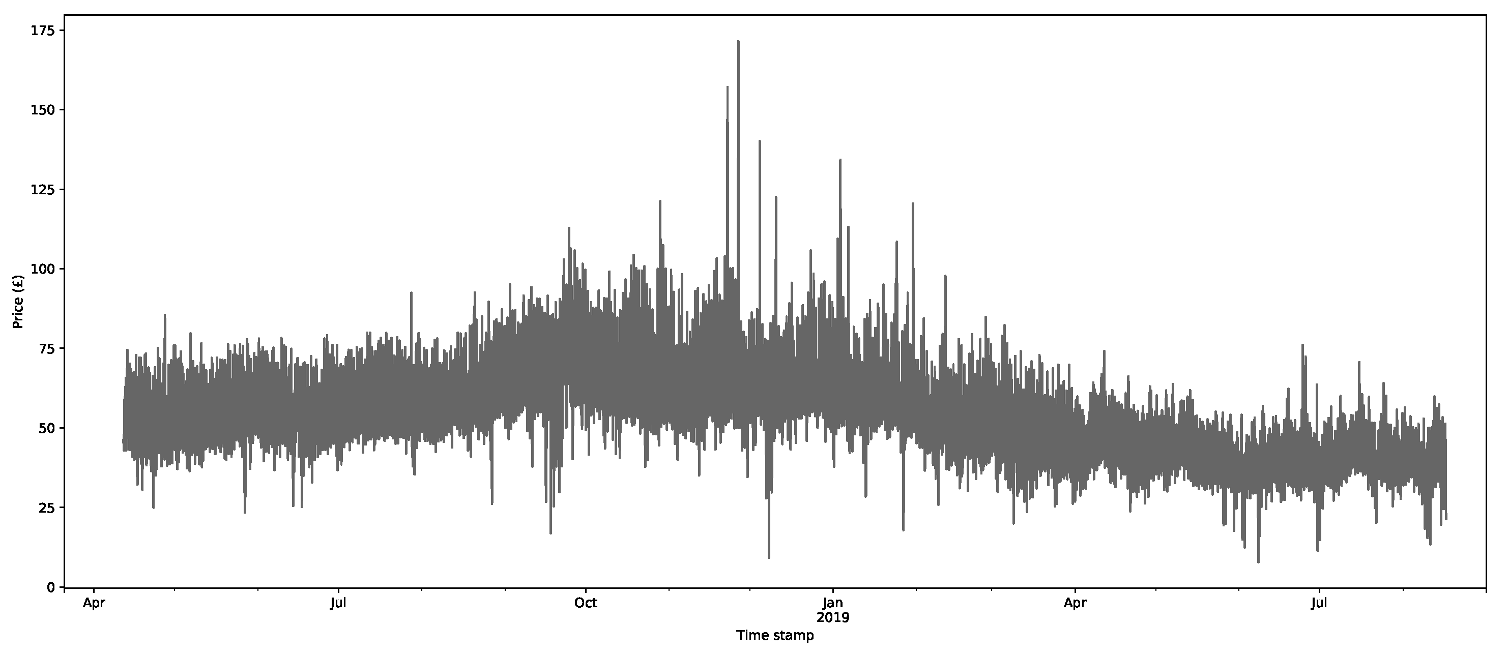
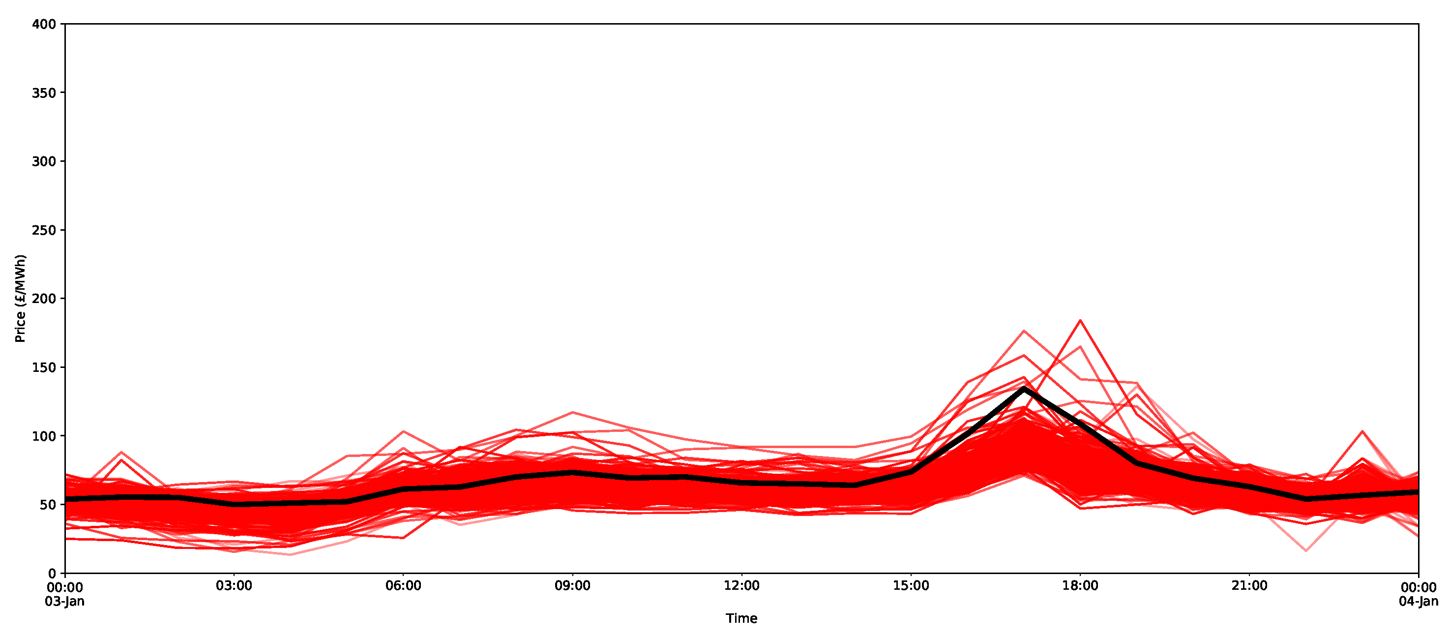
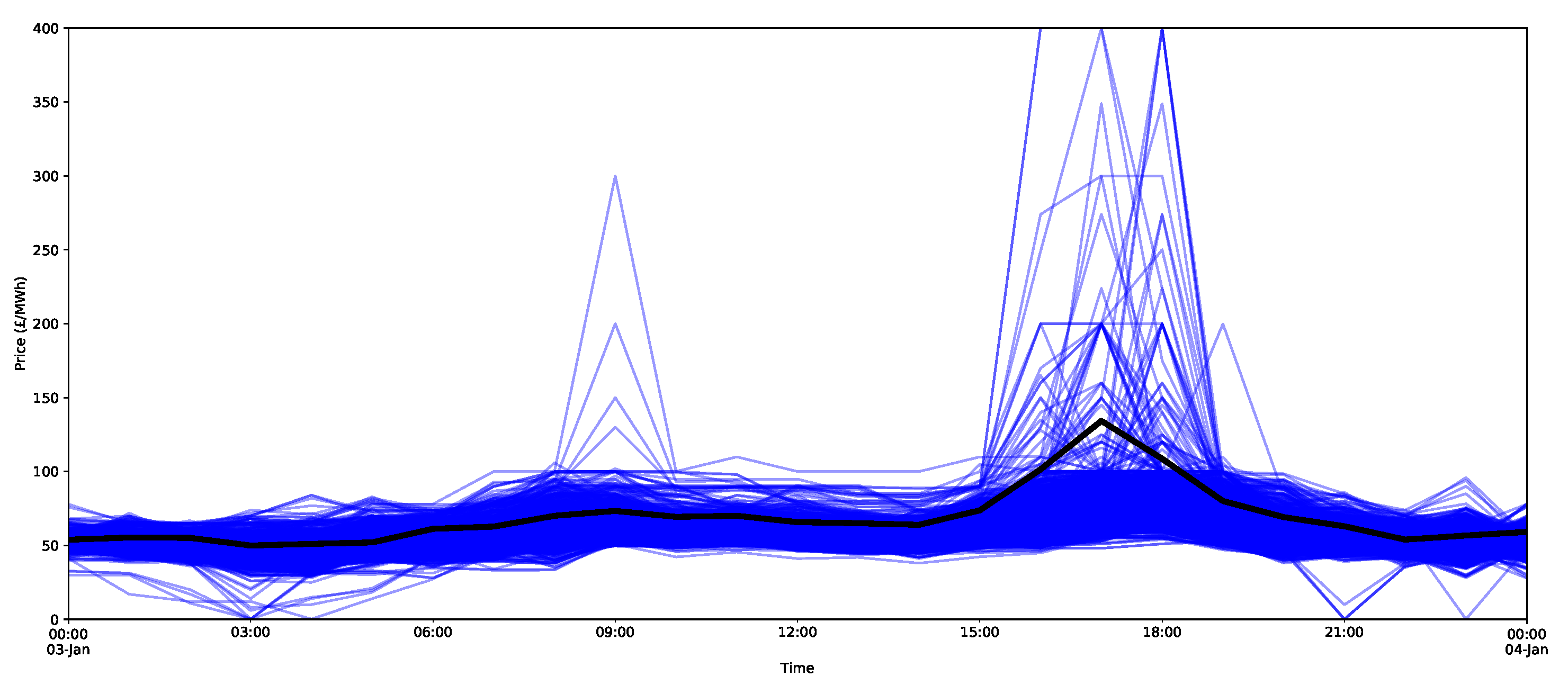
The core inputs for the model are the aggregate supply and demand curves for the GB’s market through EPEX SPOT (https://webshop.eex-group.com/epex-spot-public-market-data (las accessed on 10 August 2021)). The clearing price and volumes are created through the intersection of these curves, as described in Appendix A.1. The data were available for this trial from 11 April 2018. The estimated clearing price and volumes, as calculated via the interpolation method described in Appendix A.1, are presented in Figure 3 and Figure 4, respectively, for the period 11 April 2018 to 17 August 2019.
As noted in Section 2, there are specific rules for the bids in the EPEX market, such as maximum bids of 3000 EUR per MWh and a minimum of −500 EUR, as well as a minimum price and volume increment of 0.1 EUR/MWh and 0.1 MW. However, the data provided for this research are in GBP, which means that some modifications to the original X-model implementation are required (see Section 3.1 and Appendix A.2).
4.2. Solar and Wind Generation Forecasts
The other core dataset consists of the solar, offshore wind, and onshore wind generation forecasts. This was extracted from the Balancing Mechanism Reporting Service (BMRS) website (provided under the BMRS data license: https://www.elexon.co.uk/data/balancing-mechanism-reporting-agent/copyright-licence-bmrs-data/ (last accessed on 10 August 2021)). These are a key component of the “merit-order effect” (this is a lowering of the electricity prices due to increasing renewables, since they have no operation costs and, hence, produce relatively cheap electricity compared to other forms of generation). For example, in the supply curve (Figure 1), the first bids in the ordered list of bids are often associated with renewable generation and push more conventional generation further down in the ordered list of bids.
The hourly day-ahead solar, offshore wind, and onshore wind generation data are available through the balancing mechanism reports provided by Elexon (https://www.bmreports.com/bmrs/?q=generation/ (last accessed on 26 August 2021)). These were collected using a BMRS wrapper tool (available here: https://pypi.org/project/ElexonDataPortal/1.0.0/ (last accessed on 26 August 2021)). A sample of each of these time series is shown in Figure 5 for the same period as that of the price estimates in Figure 3. These are transparency data and are therefore available for the purposes of balancing; they must be received no later than 17:00 GMT on the day before the actual delivery. The day-ahead wholesale market auction closes at 11 a.m., which means that these data may not be available, although there are also generation forecasts with longer forecast horizons that could be used, but they would be less accurate. For this report, these forecasts are sufficient for illustrating the models. The practicality of including the day-ahead generation forecasts can be considered in future work.
4.3. Data Pre-Processing
The clearing prices in the wholesale market data were checked to confirm that they were consistent with the Nordpool data (https://www.nordpoolgroup.com/Market-data1/GB/Auction-prices/UK/Hourly/?view=table (last accessed on 26 August 2021)). The wholesale price data were available from 1 January 2017 and did not have any gaps or obvious errors. The renewable day-ahead generation forecasts had some gaps after 18 August 2019. For this reason, it was decided not to use any data after 17 August 2019, which was where the best-quality data were available. This gave a total of 959 days, which should be sufficient for splitting the data into reasonably sized training and testing sets (Section 4.4).
The main pre-processing required was the transformation of the data into 24 hourly settlement periods by correcting for the daylight savings periods. For this, a standard technique was employed: Extra hours were deleted, and missing hours were inserted by repeating the following available hour.
4.4. Splitting the Data for Training and Testing
The data were split so that the training data were any data prior to January 1 2019, and the test set was anything on or after 1 January 2019. This provided eight months of testing data and 2 years of training data. This also allowed the analysis of some of the peak prices that occurred in January 2019. Ideally, the training should be rolling and, hence, updated with the forecasts. However, this was too computationally expensive for this particular trial. If the model is developed further, methods for making it more efficient will be necessary.
5. Developing the X-Model
5.1. Volume Classes and Class Forecasts
In this trial, an example was considered that used 16 classes each for the supply and demand. This allowed the trial to be analogous to the application used in [1]. The data spanned the period of 1 January 2017 to 17 August 2019. The training set was defined to be all of the data prior to 1 January 2019, and the test set was anything from and including 1 January 2019.
The final price classes (GBP/MWh) are defined as follows.
| For demand | ||||||||
| Class | D_C0 | D_C1 | D_C2 | D_C3 | D_C4 | D_C5 | D_C6 | D_C7 |
| Value (GBP) | 100.1 | 74.5 | 64.9 | 59.1 | 54.8 | 51.2 | 48.1 | 45.0 |
| Class | D_C8 | D_C9 | D_C10 | D_C11 | D_C12 | D_C13 | D_C14 | D_C15 |
| Value (GBP) | 41.9 | 38.6 | 34.8 | 30.1 | 23.1 | 8.1 | −195.0 | −466.3 |
| For supply | ||||||||
| Class | S_C0 | S_C1 | S_C2 | S_C3 | S_C4 | S_C5 | S_C6 | S_C7 |
| Value (GBP) | 22.9 | 33.9 | 38.7 | 42.3 | 45.7 | 49.1 | 52.3 | 55.6 |
| Class | S_C8 | S_C9 | S_C10 | S_C11 | S_C12 | S_C13 | S_C14 | S_C15 |
| Value (GBP) | 59.4 | 63.7 | 68.6 | 75.0 | 86.1 | 123.9 | 1499.0 | 2798.0 |
The first class (D_C0) for demand is the aggregated volume for prices greater than or equal to 100.1 GBP, and the next is anything between 100.1 and 74.5 GBP, etc. Similarly, for supply, the first class (S_C0) is anything less than 22.9 GBP, and S_C1 is the aggregated volume between 22.9 and 33.9 GBP, etc.
There is a drawback to the count method for producing the classes. Although this guarantees that there are enough volumes in each class, it means that the majority of the volumes of bids are in the first class. However, this is a minor issue because the first classes (S_C0, D_C0) are quite important for determining the overall clearing price [27].
Notice that the average prices are 50 GBP and that there are several price classes close to this value, showing the high number of bids in these intervals.
5.1.1. Examples of Class Curves
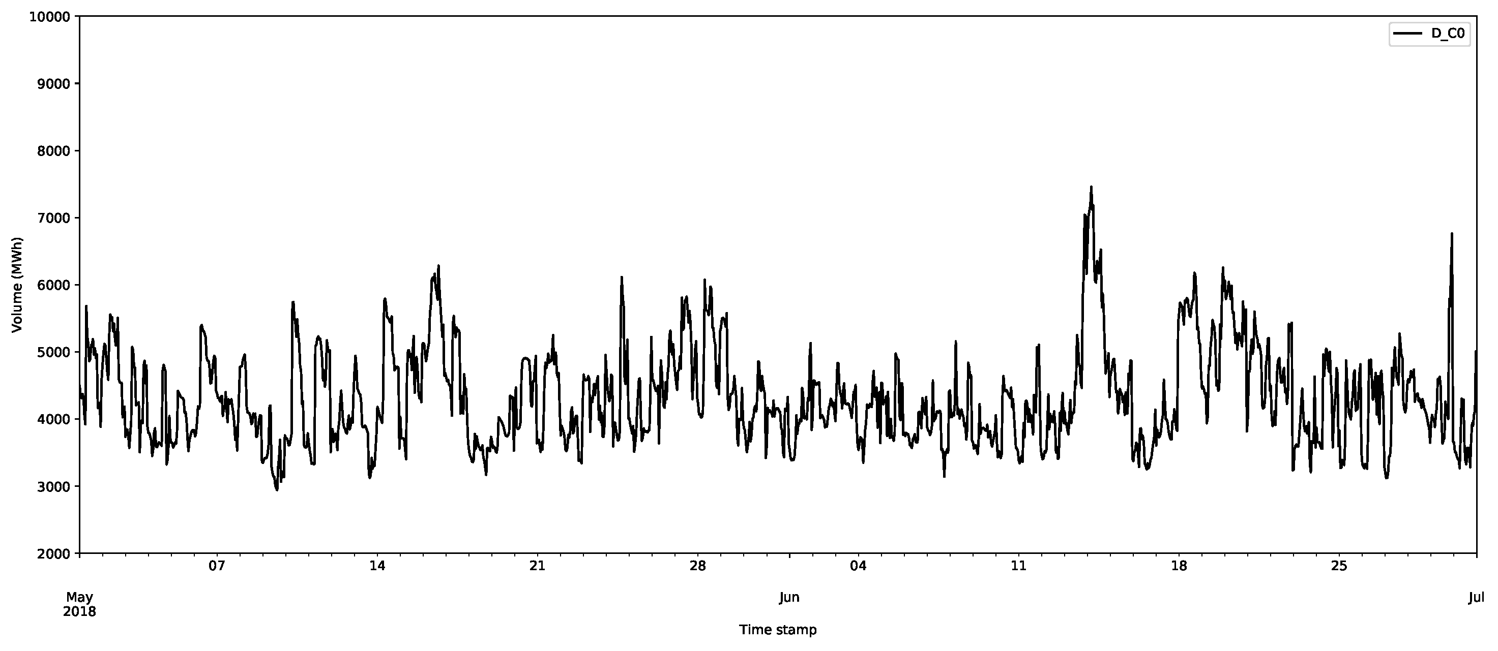
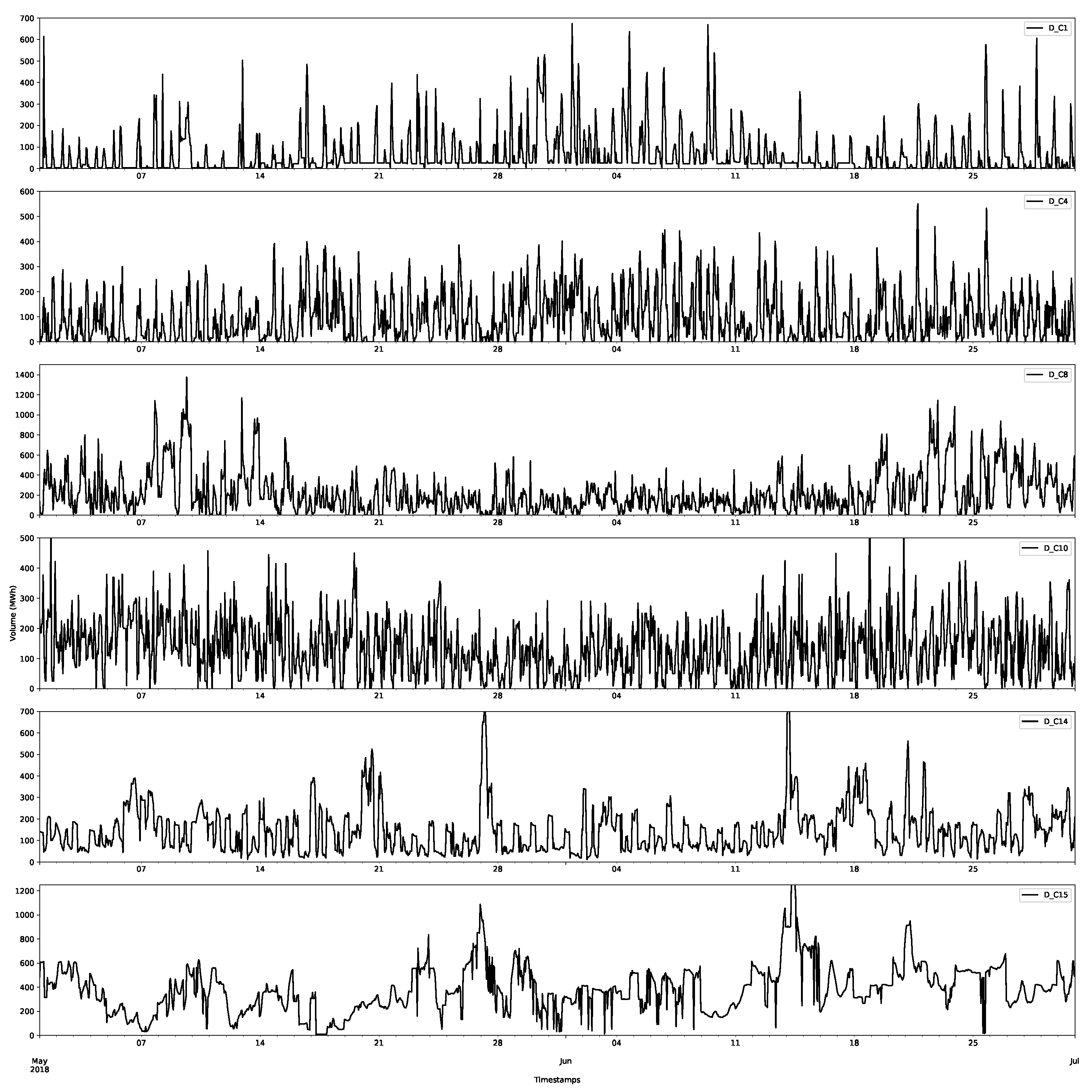
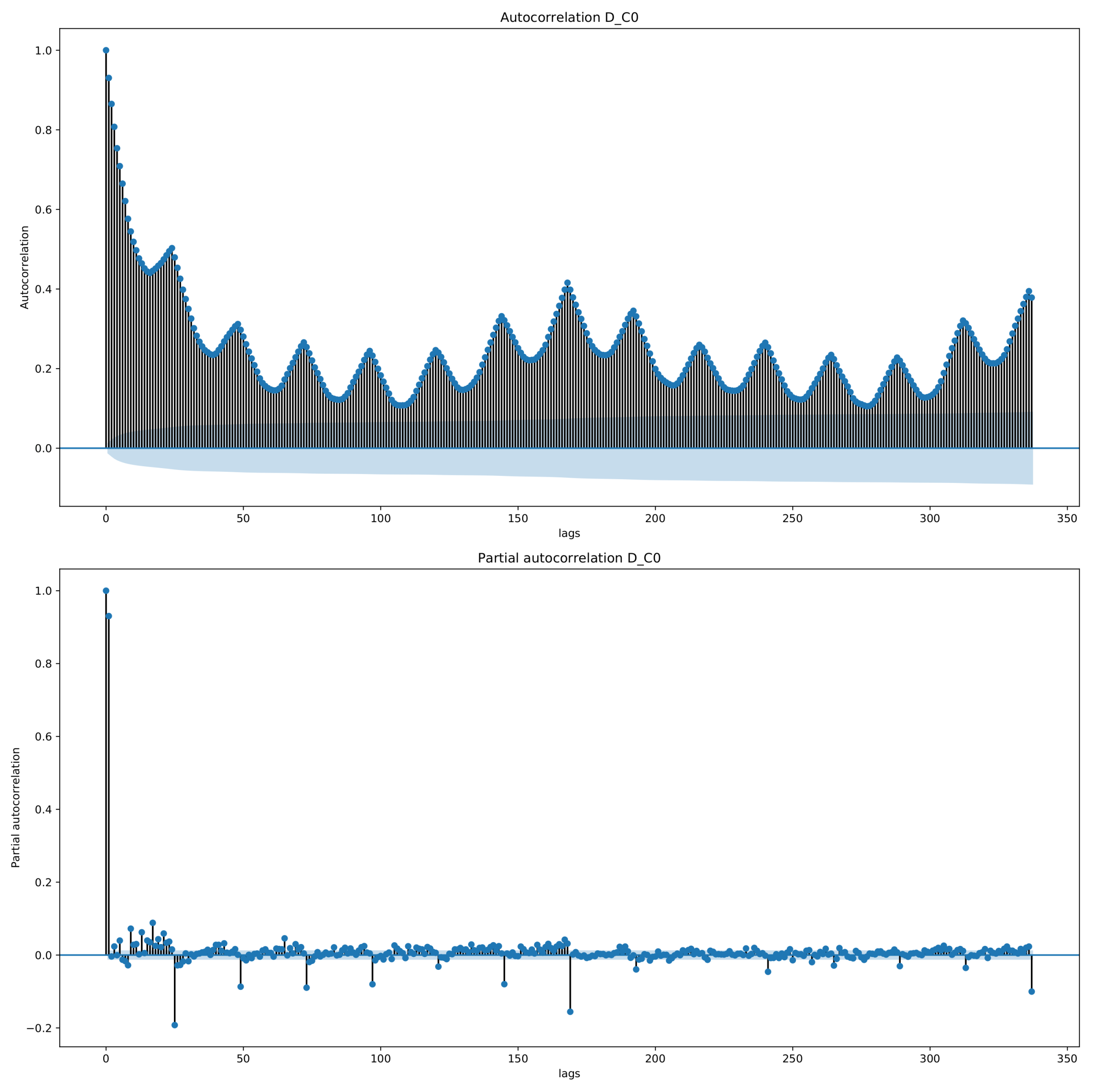
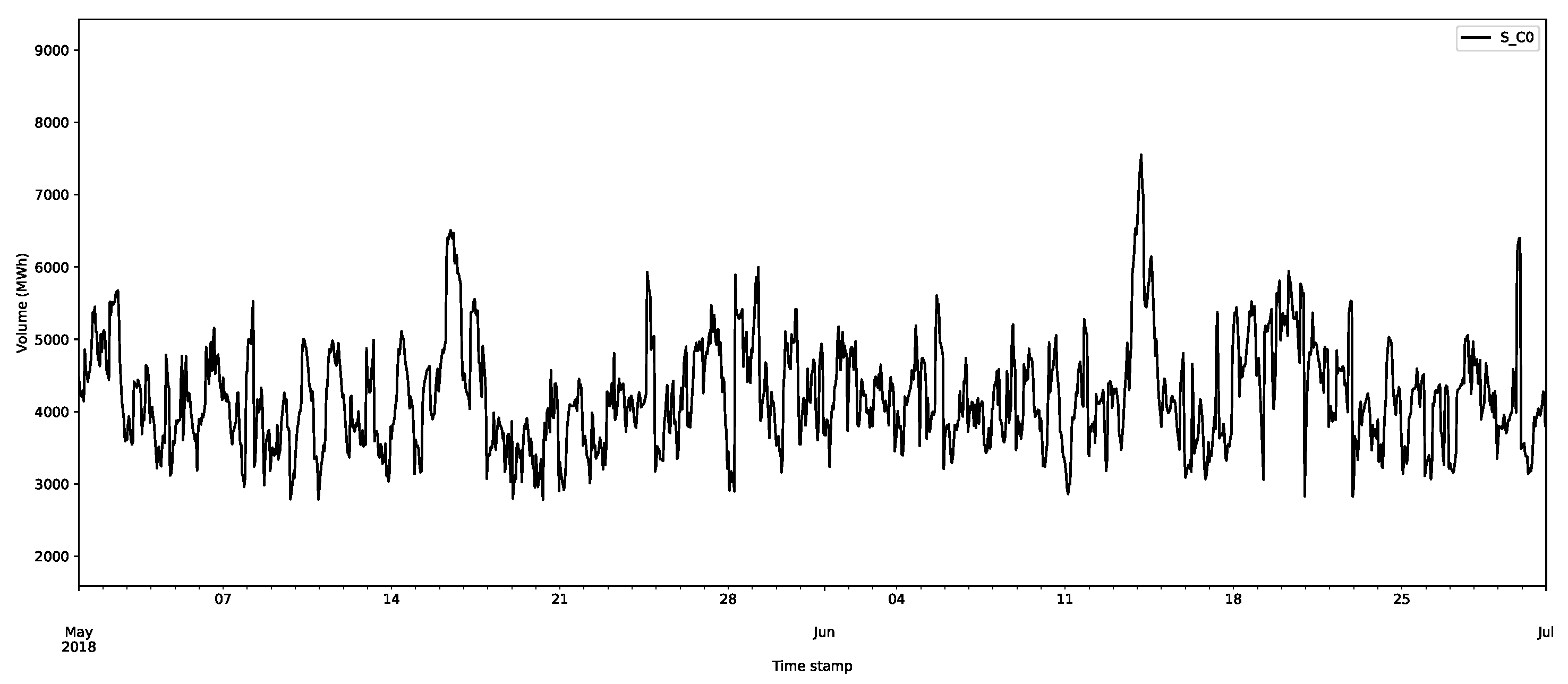
The first class D_C0 is shown in Figure 6, and selected data for other classes for the demand are shown in Figure 7. The first thing to notice is that the first class has much larger volumes than those of the other classes. In Figure 6, the largest demands are over 6000 MWh, whereas for the other classes in Figure 7, they never reach above 1500 MWh. The other things to notice are the regularities in the data; there are daily and weekly periodicities, as confirmed by considering the autocorrelation and partial autocorrelation function plots (an example for D_C0 is shown in Figure 8).
Notice that there seems to be a less periodic structure in the large classes, which is expected, as they are likely less important for the final clearance price.
5.1.2. Examples of Class Forecasts
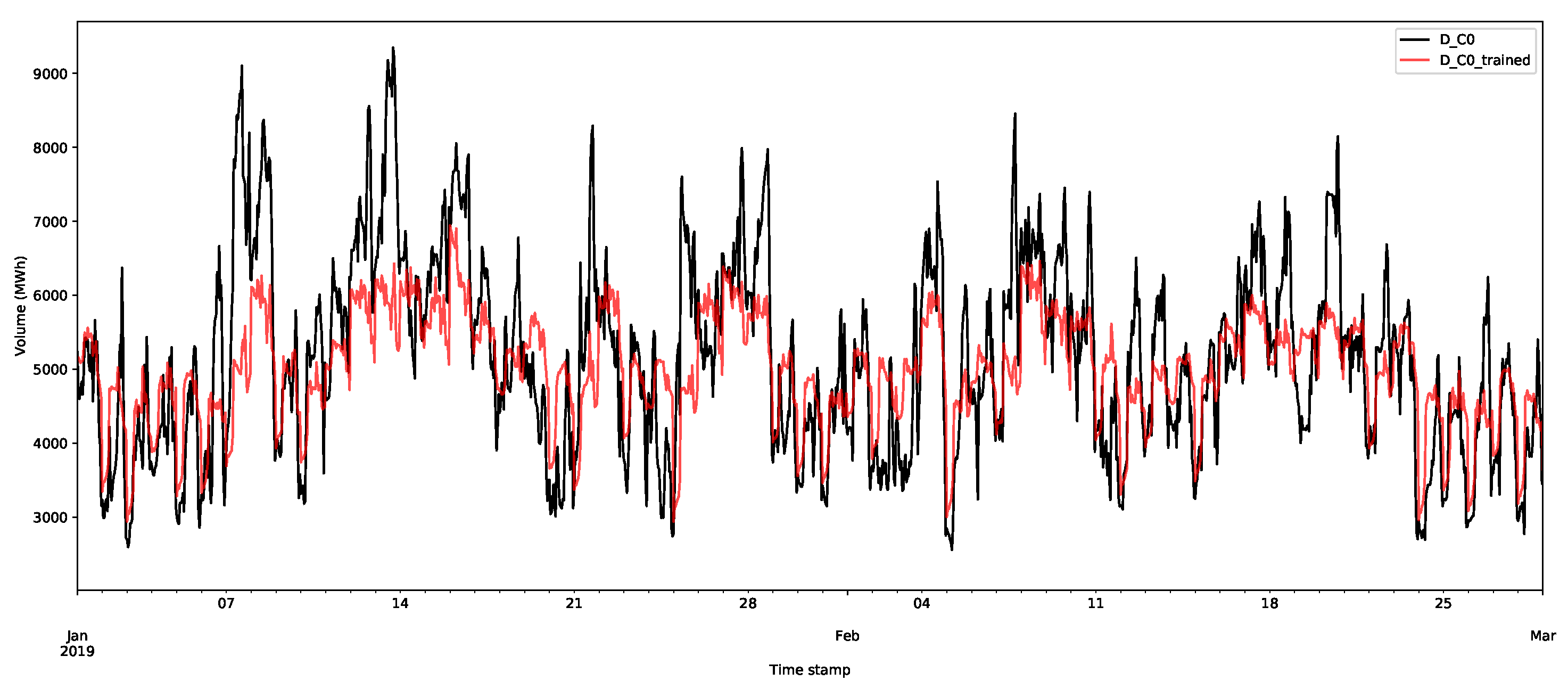
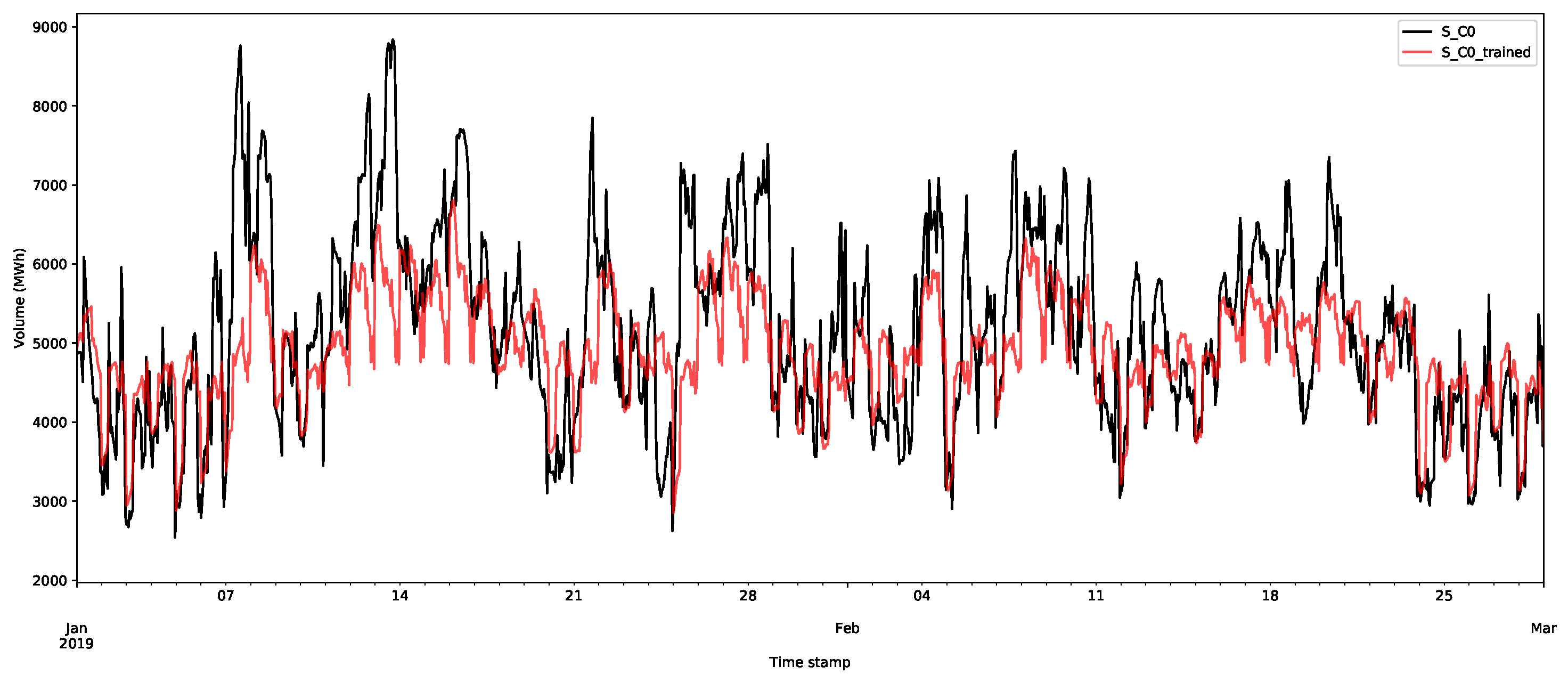
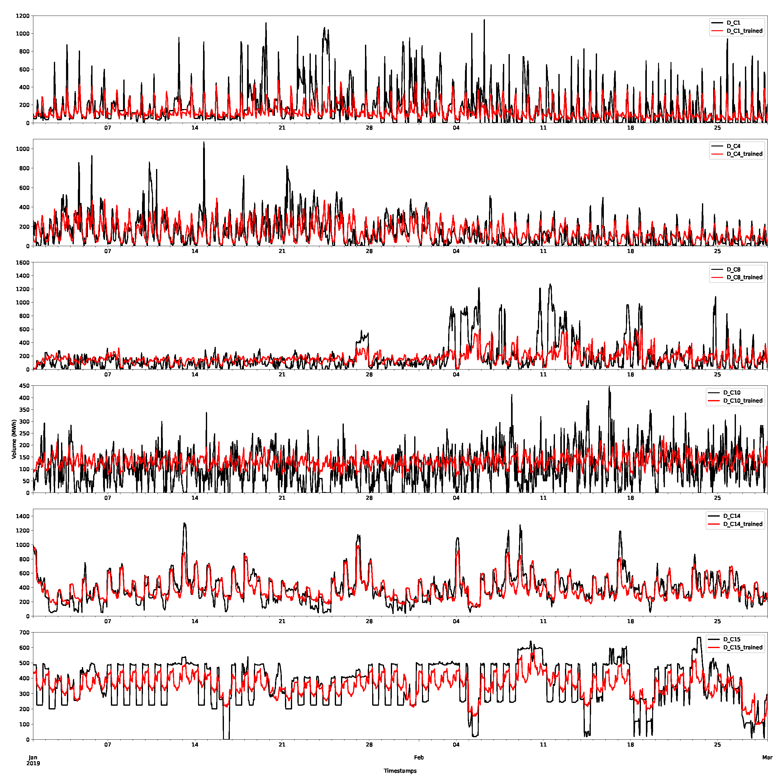
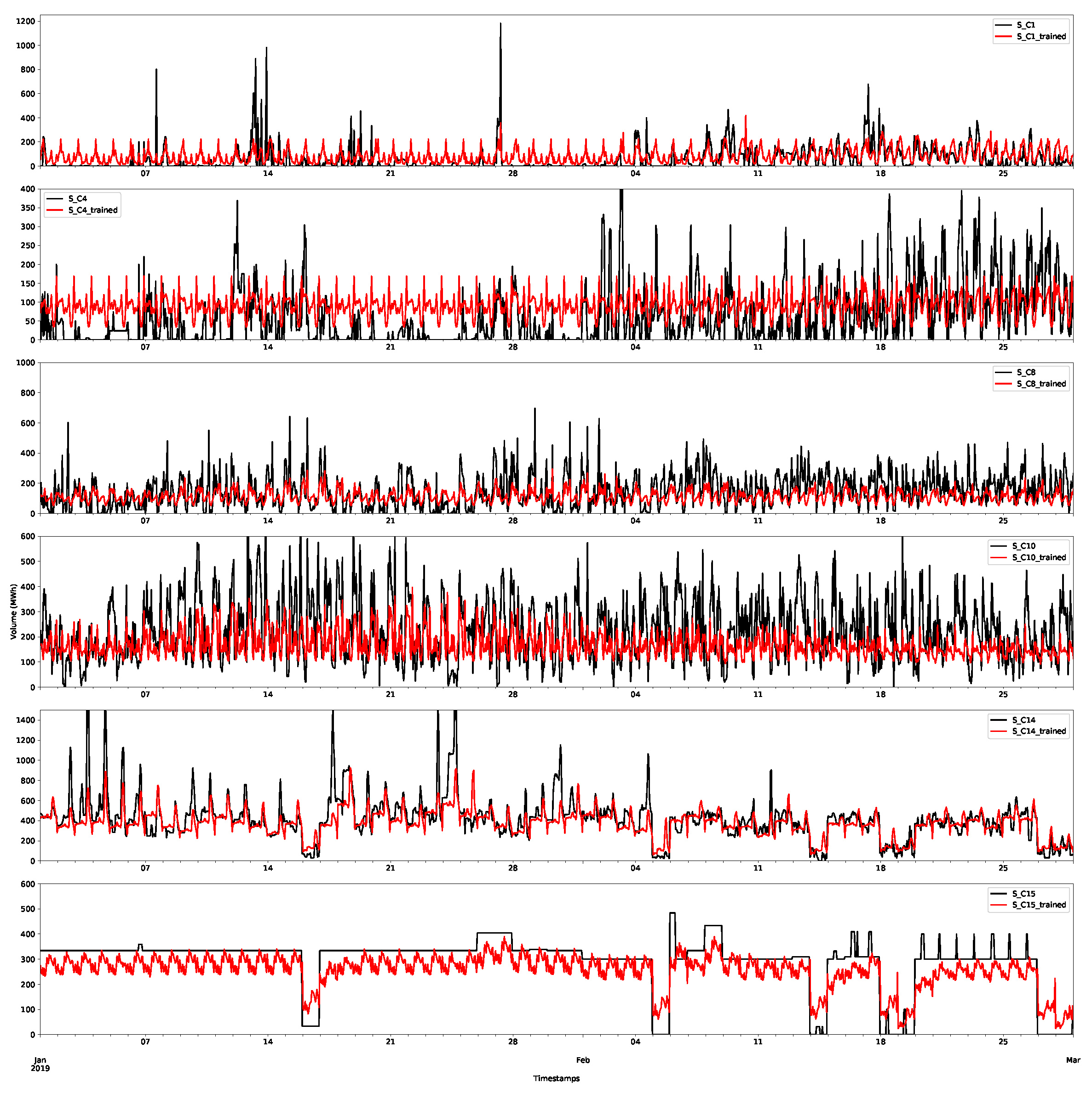
Day-ahead forecasts were produced for each of the price class using the method described in Appendix A.2.1. The class forecast for the first demand and supply classes are shown in Figure 11 and Figure 12, respectively, for the first two months (January and February 2019) of the test set. The other classes are shown in Appendix B.1. The first price classes are more regular than the other classes and, as shown in the plots, this behaviour appears to have been accurately captured. However, it is worth nothing that there are still large deviations and errors. The additional smaller volumes in this price class seem to be more accurately captured by the forecast than larger volumes. This highlights that a probabilistic approach is preferable, since it will capture more of the variations in the volumes. Some of these deviations will be captured in the residual bootstrap implementation (see Appendix A.2.3).
6. Results
This section will briefly describe some of the results for both the point and probabilistic forecasts, as well as their comparison with the benchmarks. As mentioned in Section 5.1, for the X-model, the supply and demand volumes were split into 16 price classes each, and linear day-ahead forecast models were trained on the hourly data from 1 January 2017 to 1 January 2019; these were then applied in a rolling manner to the testing dataset from 1 January 2019 to 17 August 2019, starting at midnight on 1 January. The price classes are presented in Section 5.1 and the methods for generating the X-model forecasts are explained in detail in Appendix A.2. The other methods only use the historical prices and, in the case of the ARX model, wind and solar generation forecast data.
6.1. Point Forecasts
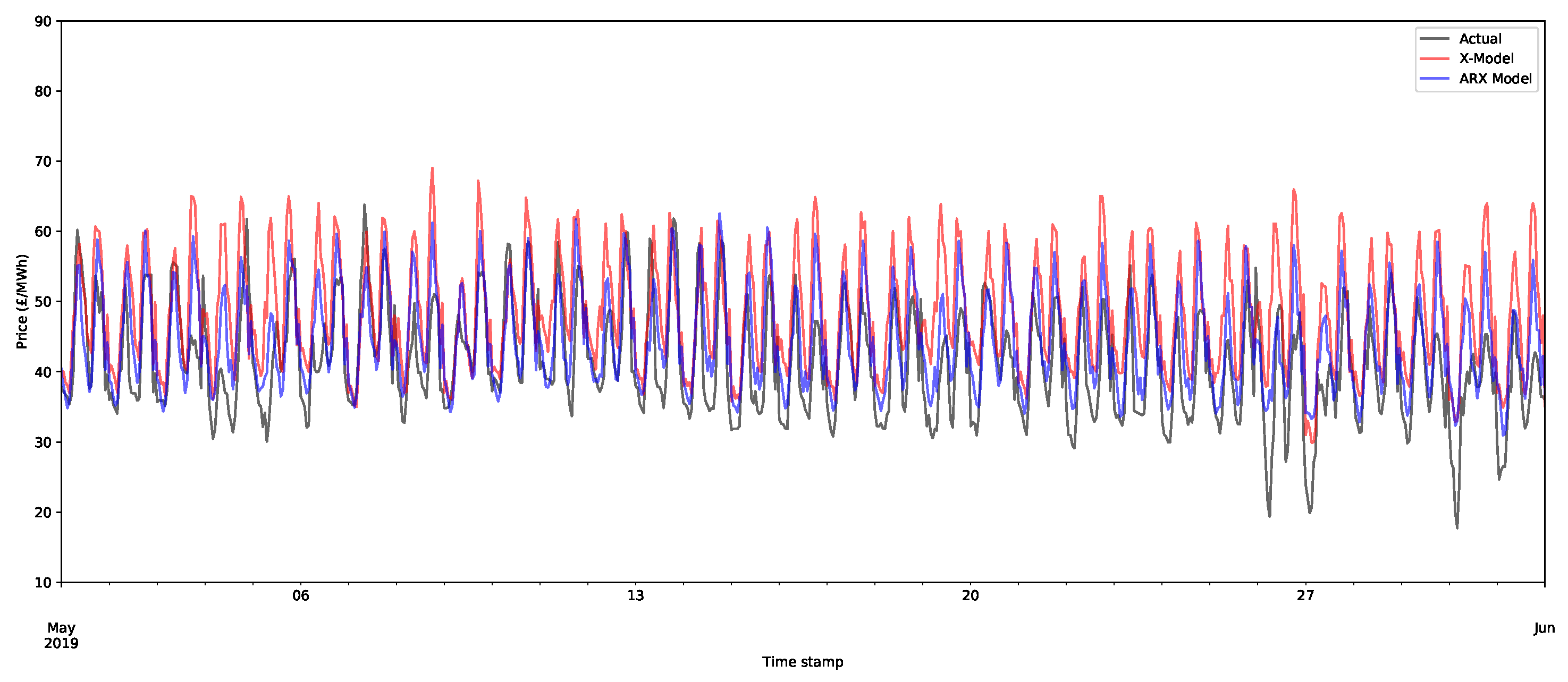
Although point forecasts are not the aim of the models, it is worth investigating them to begin to better understand some of the features of the models. An X-model point forecast model was produced by reconstructing the supply and demand curves from their class forecasts and then calculating the intersection of the two lines. An example of the day-ahead price forecasts is shown in Figure 13 for the X-model and the ARX model for the first month of the training set. As can be seen, the forecasts appear to be closely aligned to the actual data, although some of the peaks are inaccurately estimated.
For later months, the forecasts still appear to be doing a decent job of capturing the main shape of the demand, but there is a slight deviation from the average level of demand. This is illustrated for the fifth month of the test set (May 2019) in Figure 14. The main cause of this is that the models need retraining. Both the X-model and ARX model potentially use a large number of inputs, many of which can be relatively old (up to 36 days). Hence, these models can be improved by retraining on more recent data with respect to the periods being forecasted. Due to time constraints, these were not applied for this test case.
The RMSE (for the definition of the RMSE, see Section 3.5) for the daily seasonal persistence (Section 3.4) for each forecast model is shown in Table 1. It is clear now that the ARIMAX model produces the best error measures, but is very similar in accuracy to the ARX model. The X-model even has larger RMSE values than the daily persistence. As will be shown later, this is due to the bias in the data, especially for the later months. Although this paper was applied to the German and Austrian electricity market, we can compare the performance of the X-model with the performance in the original X-model paper relative to a simple persistence model [1]. In the original paper, the X-model was, in fact, better in comparison with the weekly persistence model and was 44% of the size. In contrast, our X-model is actually larger than the daily persistence model. In addition, our autoregressive model is 80% of the persistence model, but it was 57% in the original X-model paper. One reason for the lower performance of both the ARX model and X-model compared to the persistence model is likely the lack of use of conventional generation as an input. In addition, more frequent retraining of the model parameters could be another reason for the difference.
The errors broken down by month are shown in Table 2. The ARX model performs the best in the earliest month, but is the second-best model for the later months of the test set. Similarly, the X-model also has a decrease in accuracy in the later months, highlighting the need to retrain the model. In fact, the average error over the January and February months shows that, in this case, the X-model is at least as competitive as the persistence benchmark.
The ARIMAX model has relatively few parameters that use only quite recent information. This means that it is not unduly affected by seasonal effects or old data. In contrast, the ARX model and X-model not only use generation data, but they potentially also use large amounts of lagged data—up to 36 days in some cases. In a future study, it would be worth experimenting with reduced input variables to make these models more accurate when the training data are scarce (another experiment was performed with the ARX model with fewer lags, which did indeed improve the accuracy of the point forecast; however, this reduced the probabilistic accuracy, as it likely reduced the sample of residuals, the source of variation in the bootstrap forecast method.).
6.2. Probabilistic Forecasts
Probabilistic forecasts contain estimates about the distribution of the prices rather than giving a single estimated value. There are two stochastic elements that contribute to the generation of the probabilistic forecasts in the X-model. One component is Bernoulli random number generation in the reconstruction of the supply and demand curves. On its own, this is not expected to play much of a part in modelling the uncertainty. For one, the available data are currently relatively small, and hence, many of the prices will have no volumes offered or bid upon in the auction; thus, there may be very few changes based on the Bernoulli random draws (see Appendix A.2.2 for details). Secondly, the reconstruction has a limited effect, as it only influences the classes that are close to the intersection price. To illustrate this, an example of three reconstructions of the price forecasts is given in Figure 15 over 15 days of the test set. In black are the actual prices, the threshold reconstruction is in blue (in other words, that which was used to produce the point forecasts in Section 6.1 and described in Appendix A.2.2), and two examples of reconstructed curves using the Bernoulli random sampling are shown, as described in detail in Appendix A.2.2. As the figure shows, they are all quite similar, with minimal deviations from each other.
The main contributor to the probabilistic forecasts is from bootstrapping from the residuals (i.e., the deviation of the observations and the trained model) in the historical dataset. As described in Appendix A.2.2, full days are sampled (as well as across classes for the X-model) to retain any interdependencies in the data. The bootstraps are calculated for the 0.05-quantiles (ventiles) for each time step in the test set. The error score for each time step in the test set is then calculated using the pinball loss score (see Section 3.5 for details). In this example, 2000 bootstraps are used.
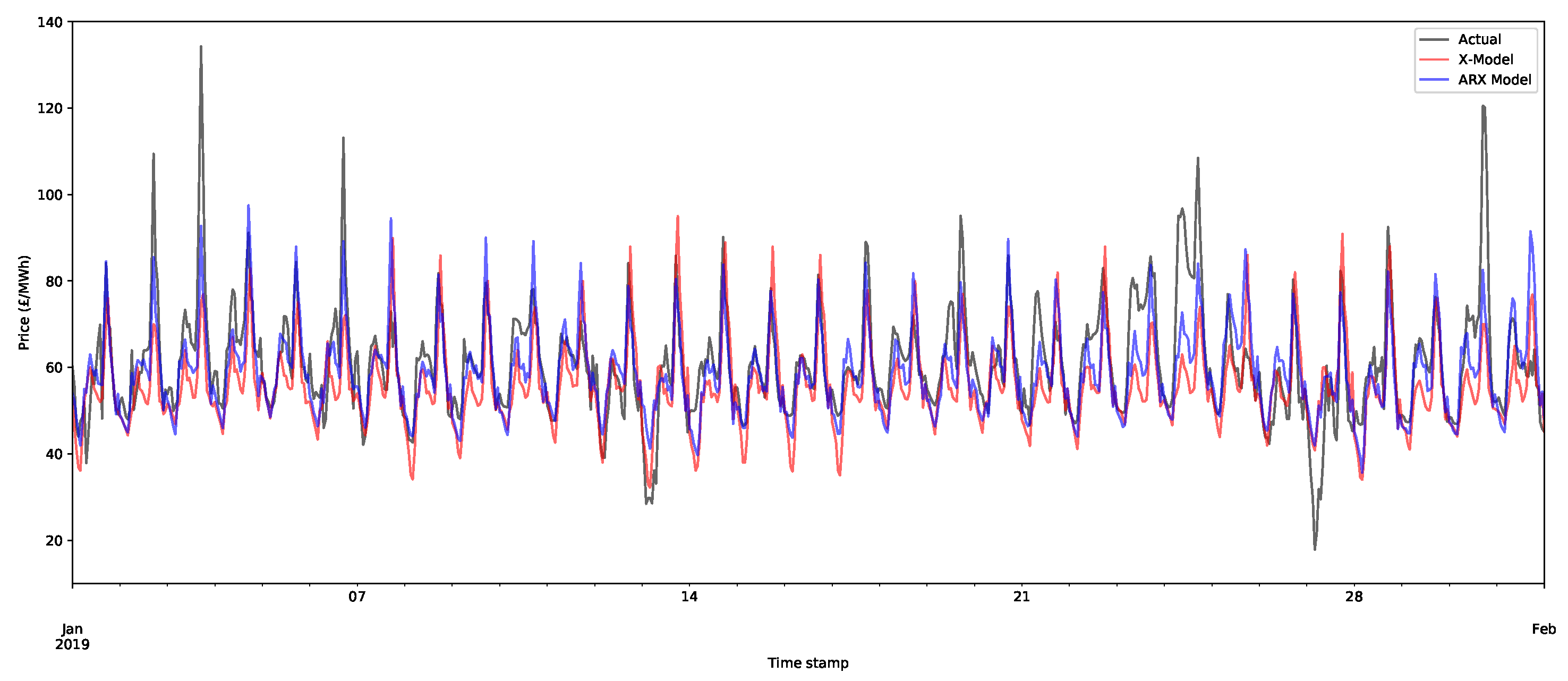
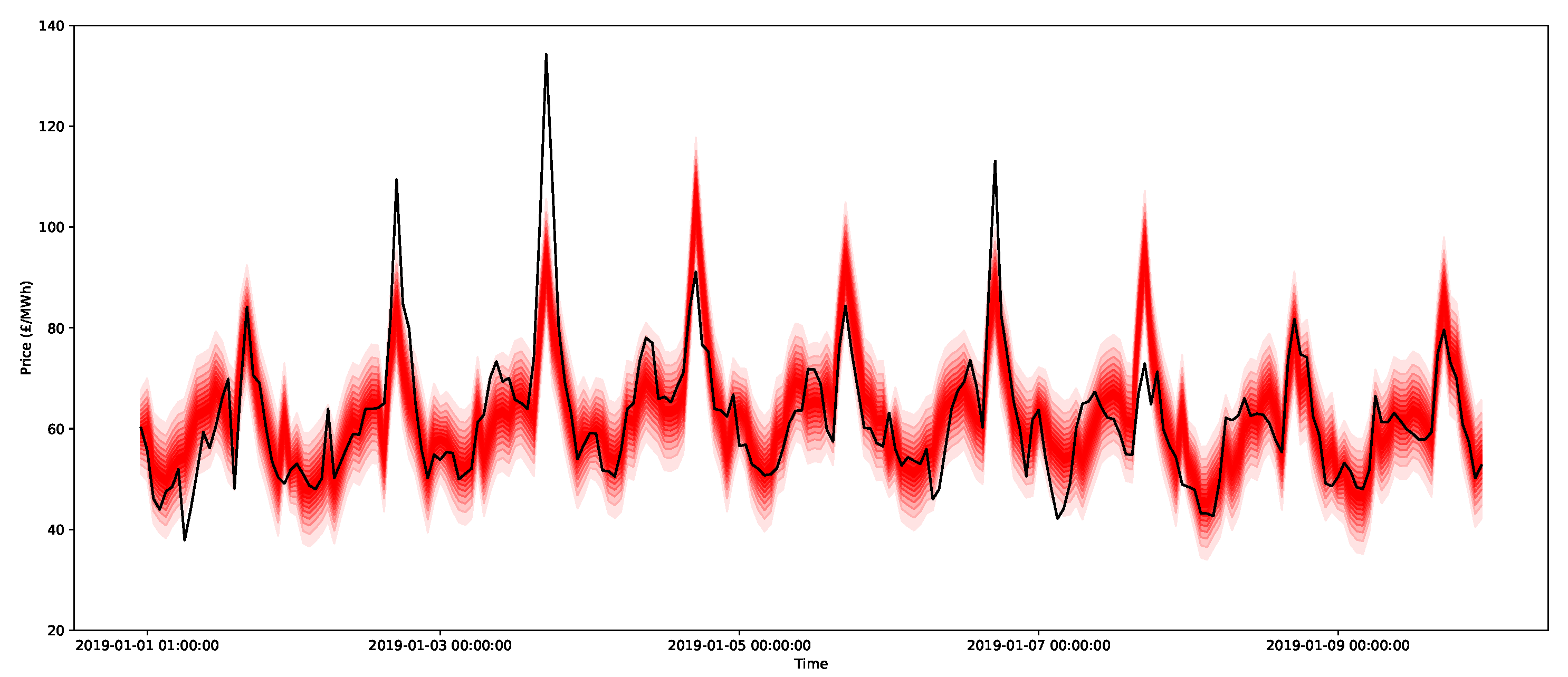
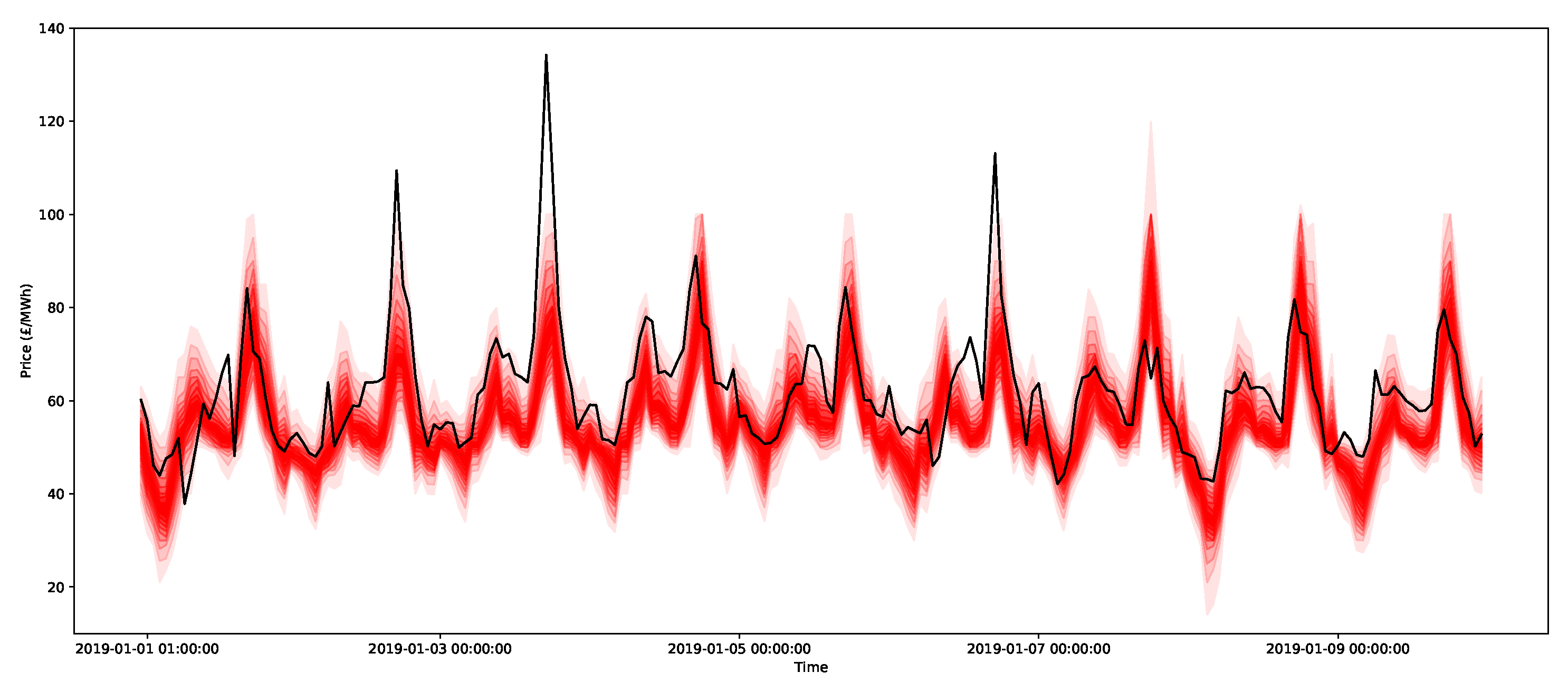
An example of the 0.05-quantiles (or ventiles) for the day-ahead forecasts for nine days for the three methods is presented in Figure 16, Figure 17 and Figure 18 for the ARIMAX model, ARX model, and X-model, respectively. The different shades represent the different predictive intervals between ventiles, where the darkest shade is for the middle ventiles (50–55 percentile and 45–50 percentiles), with gradually lighter shades until the outer ventiles (90–95 percentile and 5–10 percentiles). Comparing the ARIMAX and ARX models, one of the most clear differences is that the bounds of ARIMAX are a little bit wider, which is likely due to the restriction on the bounds being from a Gaussian distribution, which is relatively broad. However, compared to the X-model, the distributions for the ARIMAX and ARX models are much more regular and similar from one day to the next. These plots highlight some interesting features. First, it is clear that the ARIMAX and ARX models provide the most stable forecasts and express regularity from one day to the next. The X-model in Figure 18 shows much more varied distribution shapes, such as the low-cost spike that occurs between 7 and 9 January. This is likely due to the incorporation of the sensitivities in the intersection point of the supply and demand curves, which will be shown in more detail in the next section.
The average pinball scores over the entire test period are shown in Table 3. The ARX model is the best-scoring method. Once again, the ARIMAX model is one of the best-scoring models, and its score is slightly higher than that of the ARX model, although they are not significantly different. The X-model’s pinball score is about 50% higher than that of the ARX model, and is hence considered the least accurate when using this measure. As we will show later, this is likely due to bias in the estimate.
For completeness, the average pinball scores are also shown in Table 4 for each complete month in the test set and for each of the three methods. Notice that the scores of all three methods are similar for January 2019. This is the month right after the end of the training set. Further, the X-model is relatively competitive with the other models for January and February 2019. This again suggests that a large factor in the X-model’s reduction in accuracy is the requirement of more frequently retraining on more recent data. The ARX model is the most accurate model for the first four months of the test data, but then decreases in accuracy relative to the ARIMAX model starting in May 2019. This again suggests that retraining is necessary, but since the ARX model has much fewer parameters than the X-model, the reduction in accuracy occurs much later in the test set.
As shown in Section 6.1, the ARX model and X-model need retraining, as the models begin to drift for later months. Hence, the results investigated here will be for the first two months of the test set (January and February 2019). The results for the full dataset are given in Appendix B for completeness, but they confirm the bias introduced into the X-model and ARX-model for the later test data.
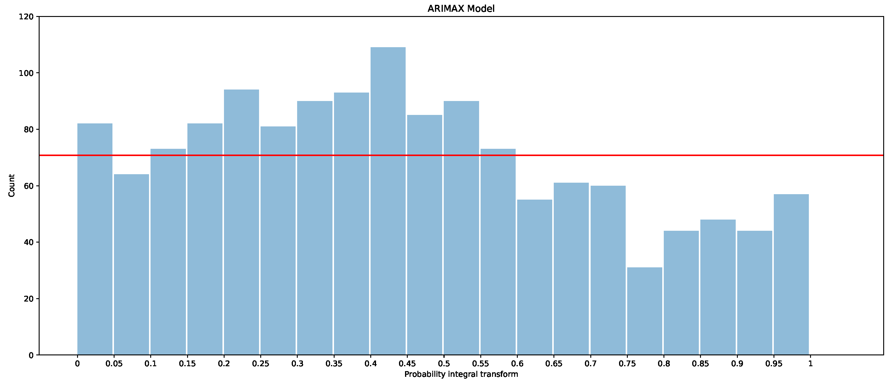
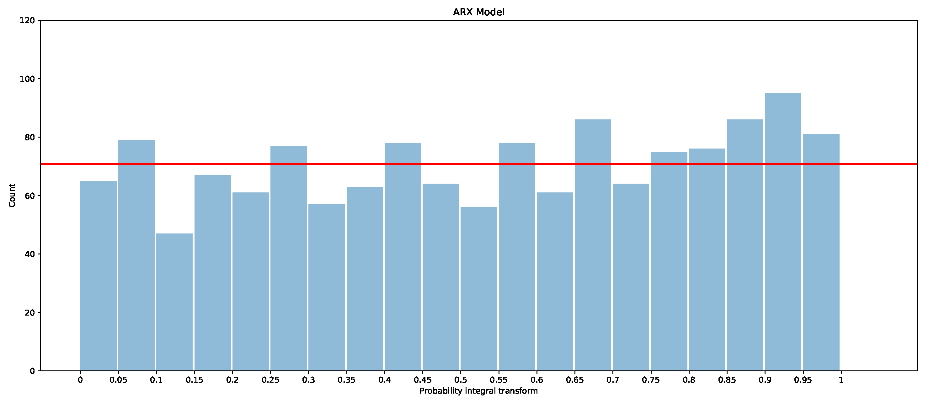
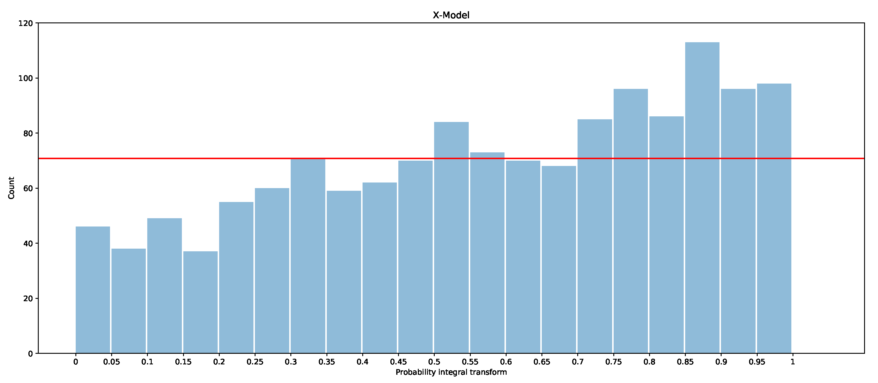
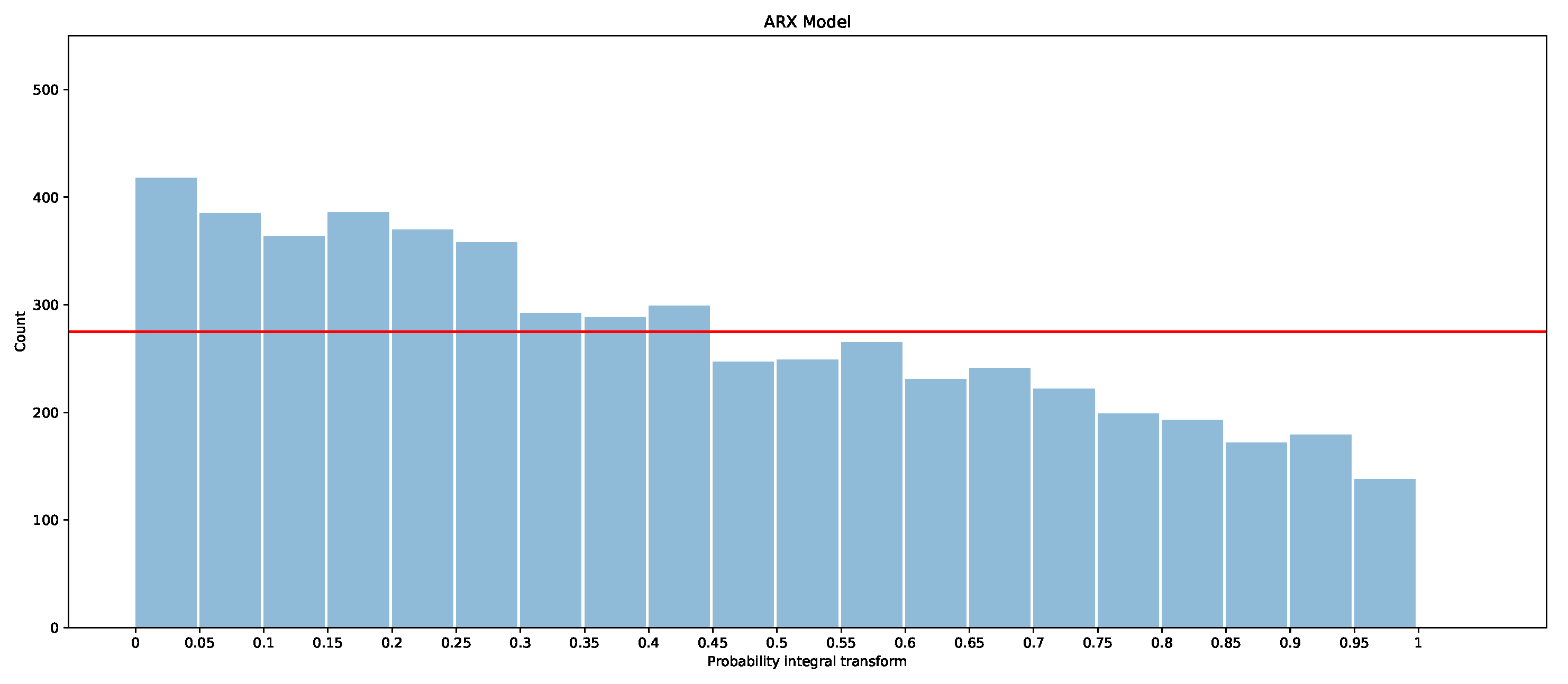
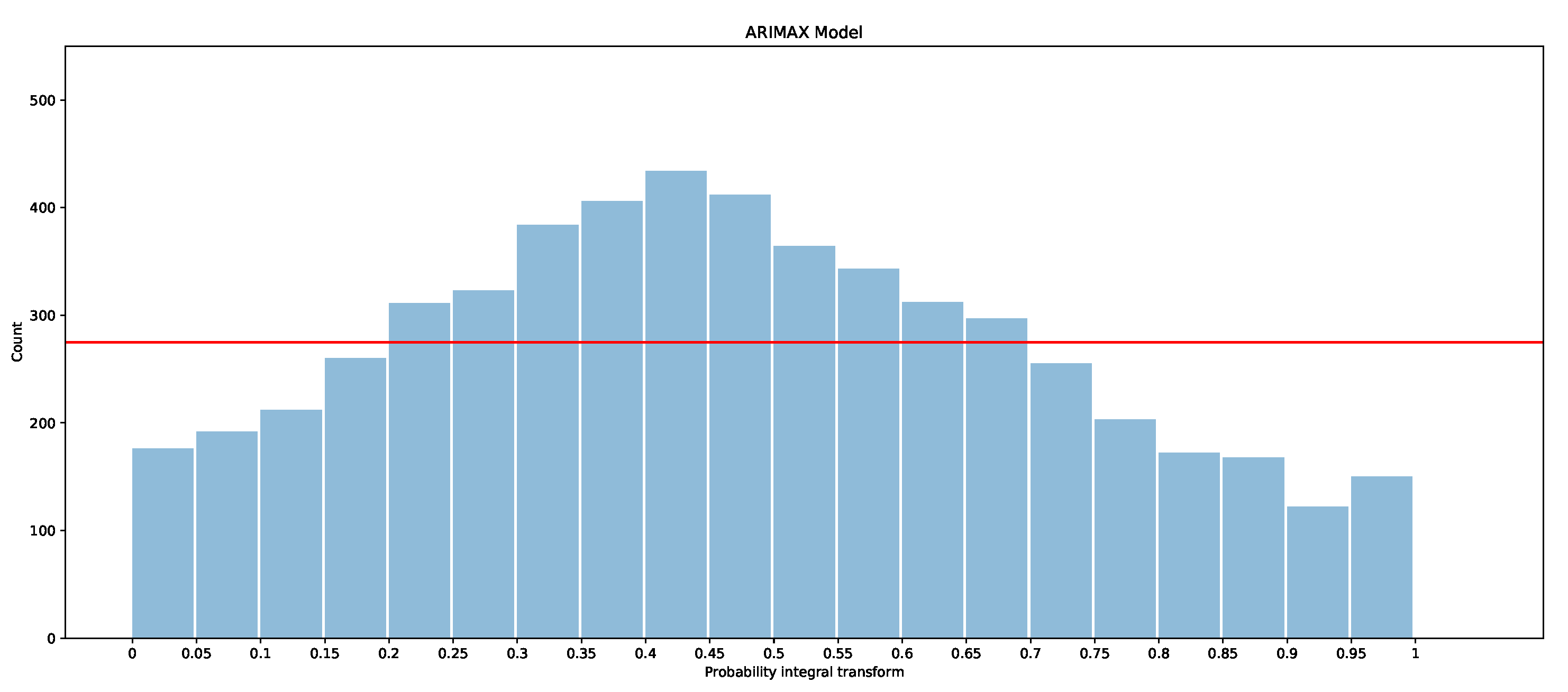
The PITs for the ARIMAX model, ARX model, and X-model are shown in Figure 19, Figure 20 and Figure 21 for the first two months of the test dataset. Additionally included is a red line with which the bars should be level if the models were to be calibrated (i.e., if all observations were evenly divided into the 20 boxes, , where is number of observations in January and February).
It is clear that the ARX model is the best calibrated of the three models, as the PIT is closer to a uniform distribution than in the other models. The ARIMAX model and X-model both have some biases, but the ARIMAX model also appears to be a little over-dispersed, which suggests that the quantiles are more spread out than the underlying distribution [28]. The X-model, on the other hand, has more observations in the larger quantiles than in the smaller quantiles. This suggests that the overall distribution estimated by the X-model is slightly shifted so that more observations fall into the larger quantiles. One explanation of the bias in the X-model is due to the use of the LASSO regressor, which is a bias estimator. This is exacerbated in the X-model, since the biases will accumulate by summing across each class forecast when producing the supply and demand curves. Comparison of the probabilistic forecasts of the original X-model papers [1,27] is difficult, as there is no proper scoring function evaluation included. However, a qualitative comparison with the probabilistic integral transforms is possible. The PIT in [1] shows that the X-model is under-dispersed with over-representation in the lower quantiles. In [27], both the X-model and the autoregression are biased and over-represent the lower quantiles. This is similarly the case for our ARX model and X-model for the entire dataset (see Appendix B.2). However, for the smaller test dataset, our models actually have an over-representation of data in the upper quantiles. The difference between the X-model in this paper and the ones in [1,27] could be because they only include renewable generation as an input rather than conventional generation, hence the bias towards lower prices (e.g., the merit-order effect). We do not produce a comparison of these results with those of the only other paper while considering the probabilistic forecasts of GB’s market [5], since they only consider prediction intervals, whereas we are interested in a wide range of quantiles—from 5% to 95%.
The PIT suggests that methods should be used to try to improve the models, such as by using a reducing bias or by scaling or shifting the estimated distributions [28]. This will be explored in future work.
6.3. Ensembles and Peak Forecasts
The quantile regressions are good for showing the uncertainty around the values produced by each model. However, each time step in the day ahead is a univariate distribution and does not explain the interdependencies in the data. The interdependencies may be more useful for an aggregator who needs to understand how the prices in one part of the day may affect other periods. The ARIMAX model does not have the capability of modelling this; hence, only the ARX and X-model are compared here.
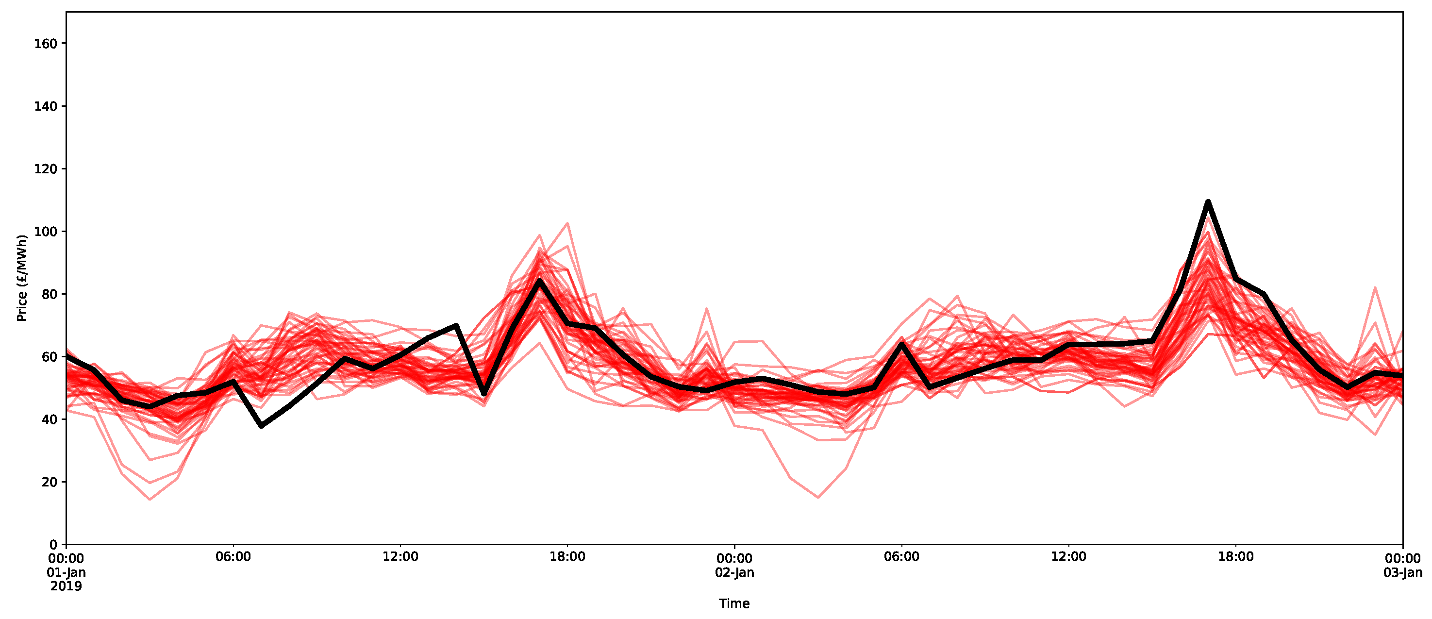
Understanding interdependencies requires estimates of a multivariate distribution for the following day. In the forecasts of the ARX model and X-model, each individual bootstrap can be viewed as an individual draw from the multivariate distribution. An example using the ARX model is shown in Figure 22, for which 50 bootstraps were randomly selected (in red). Note that the bootstraps are based on randomly sampled full daily residuals and, therefore, maintain the daily interdependencies. A similar process was performed for the X-model in Figure 23.
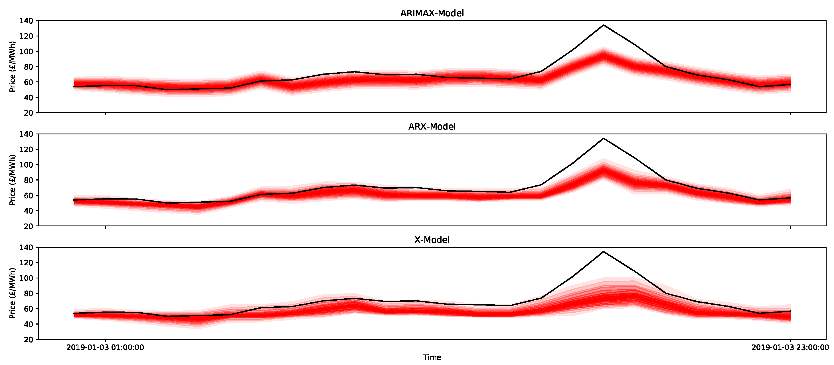
Now consider the large peak at 5 p.m. on 3 January 2019 with a size of 134.24 GBP/MWh (this can be seen in Figure 18). In addition, the surrounding hours of 4 p.m. and 6 p.m. are also very large at over 100 GBP/MWh. As indicated in Figure 24, the peak is higher than the estimates for the 95 percentile for all of the models considered, and the quantile estimates do not appear to capture the potential peak, since this extreme behaviour likely lies in the larger quantiles of the distribution (for example, the 99th percentile). Notice that, just using ventiles, the methods all score relatively poorly (in terms of the pinball score) for the peak period, as shown in Table 5. It does appear that the X-model does encompass some of the uncertainty around the higher demands surrounding the main peaks within its quantiles.
Since peaks are relatively rare, we may not expect the peaks to be captured very well, especially for the broad buckets defined by the ventiles, which were created from relatively few bootstraps (2000 bootstraps means that each bucket would only have about 100 points on average). The individual ensembles/bootstraps themselves may give more insight into these rare events.
To demonstrate the forecasts of the peaks, all 2000 bootstrap forecasts are shown for both the ARX model and the X-model in Figure 25 and Figure 26, respectively. Notice that the X-model has some ensembles with more extreme peak predictions (and note that they were not visible in the prediction interval estimates in Figure 18, since they were in the top 5% of values). Additionally notice that the adjacent time periods also have larger estimates with the X-model.
Hence, both models make it clear that there is potential for a price spike at 5 p.m., and many of the ensembles indicate a peak. An explanation for the peaks (especially the larger ones) in the X-model is offered in the original X-model paper [1], which suggests that the steepness in the gradient of the supply curve produces a sensitivity to the final clearance price.
In fact, this is seen to be the case for the 5 p.m. peak on the 3 January 2019, as shown in Figure 27 for the peak hour and selected hours around the peak period. Notice the large rate of change in the demand curve near the intersection point. A small change in the bids and offers could shift the curves, so the intersection and, hence, the clearance price could change quite dramatically. In addition, for the same hour, peaks as high as 400 GBP/MWh are predicted by the X-model (Figure 26). As shown by the supply–demand curves, such a peak is, in fact, quite possible, as a small change in the supply or demand curve could easily shift the intersection point to this extremely high price.
The potential peak of 400 GBP/MWh was not reproduced in the ensembles of the ARX model. This method only utilises the final clearance prices, so very large deviations will only be included in the residual bootstrap if they are observed as historical deviations from the model. This means that the ARX will model the typical behaviours, but is unlikely to include features due to the sensitivities in the supply and demand curves.
In contrast, the X-model is designed to forecast the supply and demand curves. The bootstrapping of the residuals is added to the forecasted price classes, creating several reconstructed supply and demand curves. Some of these pairs of curves will produce small changes, which will result in a high clearance price, as shown in this example.
The X-model process has both positive and negative implications for practitioners. On the one hand, it can highlight moments that are particularly sensitive to potential price spikes. However, at the same time, it may give a false impression of how often these occur. This suggests that one of the best usages of the X-model is in conjunction with other techniques and methods. If the X-model suggests a price spike, this should suggest to the practitioner to look deeper into the supply and demand curves estimated by the method. These should be further compared to findings with other models, such as the ARX model, to see what the typical behaviour is likely to be in order to better inform the business decisions to be made.
7. Conclusions and Discussion
The aim of this paper is to present the first implementation of a relatively new day-ahead probabilistic forecasting method for electricity prices with X-model specifically for Great Britain’s market, as well as to discuss its performance in comparison to two more common methods that were implemented in the same context and also presented in this paper. The research presented here suggested the X-model could be useful for predicting price spikes and the uncertainty around them, and a particular example from January 2019 that was examined in this report showed that the X-model correctly indicated a spike and highlighted the sensitivity of the prices at that period of time.
In addition to the X-model investigation, two other models were also tested and introduced. A simpler version of the X-model—labelled ARX here—was found to be the most accurate model, especially for probabilistic forecasting, although it may not be as useful in predicting price spikes as the X-model. An ARIMAX-type model was also introduced. This model also performed well with a small number of parameters and required less training. This suggests that if data are limited, this model would be the most suitable for standard probabilistic forecasts. However, if more data are available, then the ARX model is preferable, as it can also produce ensemble forecasts that capture the intraday day-ahead price dependencies, which could help inform decision making and could be useful for other applications.
The study of data-driven probabilistic forecasts has important implications for future energy markets and the policies that support them. Firstly, increasing numbers of trades are being algorithmically implemented (65% of EPEX SPOT trades in 2019) [29]. Hence, there is a requirement for more data-driven models, such as those presented in this paper. Secondly, localised energy markets are being emphasised as a potential solution in many marketplaces as a way to coordinate an increasingly complex decentralised energy system [30]. This will require more advanced probabilistic modelling, such as that demonstrated in this paper, in order to cope with the increasing uncertainty and irregularity in pricing at the localised level. This will also require increased data availability for the more granular demand and distributed generation. At a policy level, this may require changes in how markets are regulated. These will be important areas of investigation and research, but are beyond the scope of this paper.
Some limitations of this study include:
- Only one specific price spike event has been studied in detail, but if additional price spike events would have been identified and studied, a more quantitative conclusion on the benefits of the X-model for price spike events with respect to more traditional modelling techniques could have been reached;
- Two more traditional modelling techniques were used as benchmarks. However, these techniques were not specifically designed to handle price spike events. Additional benchmarks that consider price spike events could be informative;
- Only means of renewable energy generation (solar and wind) were considered as exogenous variables. In other studies, such as [27], conventional energy generation was also considered as an input, and it would be informative to compare the current results with those of the same techniques when including these variables.
There are several useful extensions of the models and analyses that could be included in future work. One useful extension of the research presented here is the expansion of the model to longer-term forecasts. This would improve the planning and understanding of the impact of higher proportions of renewables on the network. A medium- and long-term extension of the X-model is described in [27].
Since there are multiple components of the X-model, the algorithm presented here was not optimised for computational efficiency. Most of the components are relatively efficient, and many are only implemented once—for example, identifying the supply and demand classes. The LASSO model and, hence, the class forecasts are all relatively quick to implement. There are only two main elements that are quite computationally expensive:
- Generating the probability and average volumes for each price class.
- Generating the bootstrap forecast. This is expensive because each bootstrap also includes a stochastic reconstruction of the supply and demand curves.
The first operation is not an issue, as this can be derived offline and is only updated at irregular intervals. The second, however, is quite computationally expensive, since it requires two expensive steps for each bootstrap: first, a Bernoulli random draw for all elements in the forecast vector, and second, a calculation of the intersection of the reconstructed curves. However, each bootstrap can be calculated on its own, and hence, the code can be easily parallelised. This will be considered in future work.
Future work can also focus on the more recent evolution of the market in Great Britain. The current paper analysed a dataset collected prior to January 2021. After January 2021, the application of Brexit will slightly modify Great Britain’s individual exchange market, particularly regarding the algorithm coupling the GB’s and EU’s prices.
Author Contributions
Conceptualisation, S.H. and J.V.; Methodology, S.H. and J.C.; software, S.H. and J.C.; validation, S.H., and J.C.; formal analysis, S.H.; investigation, S.H., J.C., and J.V.; data curation, S.H.; writing—original draft preparation, S.H., J.C., and J.V.; writing—review and editing, S.H., J.C., and J.V.; visualisation, S.H. and J.C.; supervision, S.H. and J.V.; project administration, J.V.; funding acquisition, J.V. All authors have read and agreed to the published version of the manuscript.
Funding
This work was completed as part of the Energy Revolution Integration Service (ERIS) at the Energy System Catapult and was funded through the Industrial Strategy Challenge Fund via the Prospering from the Energy Revolution programme.
Institutional Review Board Statement
Not applicable.
Informed Consent Statement
Not applicable.
Data Availability Statement
The aggregated supply and demand data used here were purchased from EPEX SPOT https://webshop.eex-group.com/epex-spot-public-market-data (las accessed on 26 August 2021). The solar and wind generation forecasts are available from Elexon’s Balancing Mechanism Reporting Service, https://www.elexonportal.co.uk/category/view/10701 (last accessed on 26 August 2021), and they were extracted using the ElexonDataPortal wrapper https://github.com/OSUKED/ElexonDataPortal (last accessed on 26 August 2021) made available by OSUKED.
Acknowledgments
We would like to acknowledge several individuals who helped and supported this work—firstly, our colleagues Naomi De Silva and Alasdair Muntz, who were invaluable for their knowledge on wholesale markets. We would also like to thank Ayrton Bourn, who developed the BMRS wrapper, which was extremely valuable for ease in the extraction of the day-ahead wind and solar generation forecasts. Finally, we would like to thank EPEX SPOT for providing the data used throughout this report.
Conflicts of Interest
The authors declare no conflict of interest.
Appendix A. X-Model Details
The X-model is fully detailed in the original paper [1]; however, for completeness, some of the main features are included in more detail here.
Appendix A.1. Deriving the Prices and Volumes
As described in the main text, the market clearing price is derived from a complex EUPHEMIA algorithm that is owned by the power exchanges and calculates the prices for 25 European countries (see https://www.n-side.com/pcr-euphemia-algorithm-european-power-exchanges-price-coupling-electricity-market/ (accessed on 10 August 2021)). The details are not available, but it is known to be a relatively complex algorithm that joins the simple, block, and smart orders across multiple markets.
Since this algorithm is not available, an approximation of the true clearance price would use the intersection of the aggregated supply and demand curves from the EPEX SPOT auctions [1]. This section briefly outlines a comparison of the two methods for calculating the clearing prices and volumes using different ways of approximating the intersection of the supply and demand curves. The results of the methods are compared to the actual clearing prices.
Two different methods were considered to calculate the intersection price:
- A clearance price procedure that checks—in order—each supply offer volume to see if the corresponding bids can purchase all of the offers with the given price. The maximum of these prices is used to define the clearing price. This will be referred to as the clearing procedure, and the resultant price and volumes are referred to as the “clearance price” and “clearance volume”.
- A linear interpolation. The volumes of the supply and demand curves are interpolated to a 0.1 GBP resolution grid, and the intersection is then calculated by identifying where the price differences change signs. This gives one price estimate and two volume estimates (one above and one below the intersection, since this is based on a grid). This will be referred to as the interpolation method or procedure. The resultant prices and volumes will be referred to as the “interpolated price” and “interpolated volumes”.
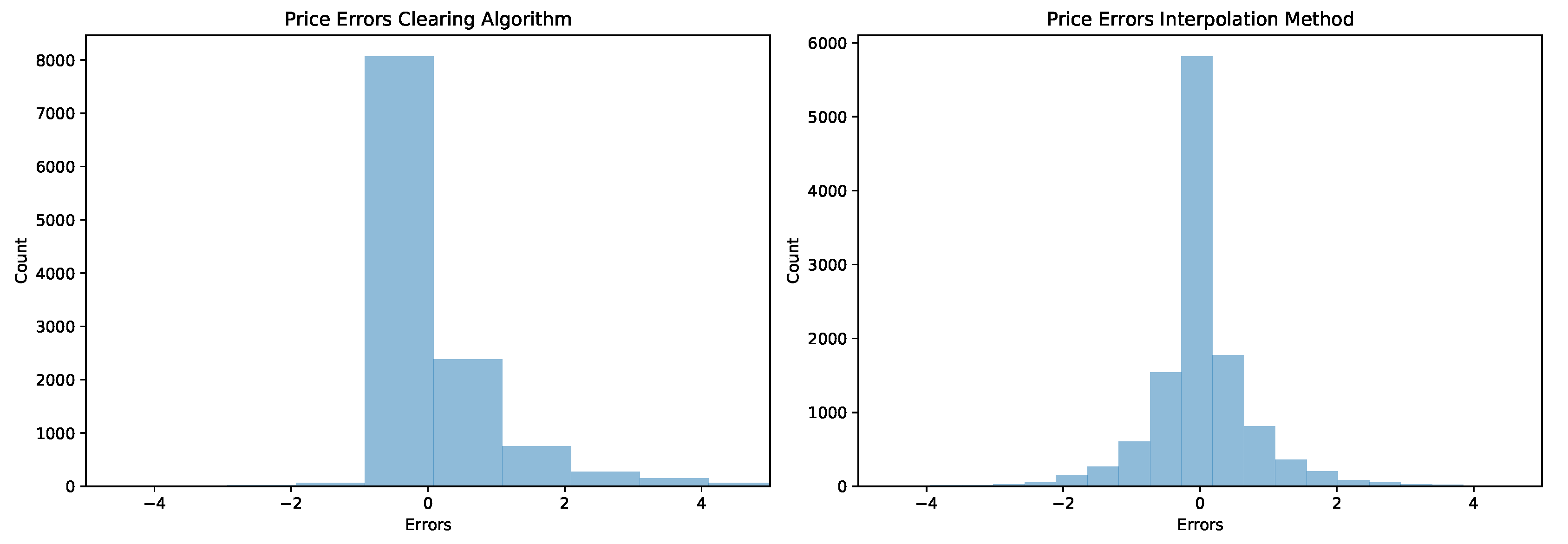
Using the actual clearing prices and volumes, as provided through EPEX SPOT, the errors (estimated minus the actual) were calculated for each method for a sample of dates (11 April 2018 to 17 August 2019). Some statistics of these errors are shown in Table A1, including the average error, the average absolute error, maximum and minimum error, and average relative error.

Table A1.
Some statistics on the errors for the two interpolation methods for April 2018 to August 2019.
Table A1.
Some statistics on the errors for the two interpolation methods for April 2018 to August 2019.
| Clearance Price (GBP) | Interpolated Price (GBP) | Clearance Volume | Interpolated Volume 1 | Interpolated Volume 2 | |
|---|---|---|---|---|---|
| Average error | 0.30 | 0.02 | −4.17 | 11.52 | 11.59 |
| Average abs error | 0.43 | 0.48 | 9.84 | 12.94 | 13.06 |
| Maximum error | 36.29 | 7.97 | 834.3 | 877.13 | 875.8 |
| Minimum error | −14 | −14.93 | −1060.3 | −999.82 | −1001.52 |
| Standard deviation of error | 1.07 | 0.81 | 40.62 | 28.93 | 29.04 |
| Average relative error (%) | 0.59 | 0.07 | −0.09 | 0.24 | 0.24 |
Beginning by considering the price errors, the interpolation method appears more accurate in terms of both the average error and the maximum absolute error (36.29 GBP for the clearance algorithm vs. 14.93 GBP for the interpolation method). The average error and average relative error show a large improvement for the interpolated method compared to the clearance method, with average errors of 2 pence compared to 30 pence, respectively. The average absolute errors are similar, since the clearance methods are skewed toward overestimating the price, as shown by comparing the histogram of the errors in Figure A1. There are a few large errors in the price, with a maximum absolute error of 14 GBP for the interpolation method and an error of over 36 GBP for the clearance algorithm. This is actually caused by an unusually large price on 31 March 2019. Despite the large errors that both methods have, on average, quite accurate estimates were obtained with only 0.6% and 0.07% relative errors for each method.
Figure A1.
Histograms with 50 bins of the errors for the two intersection methods: the clearance algorithm (left) and interpolation method (right).
Figure A1.
Histograms with 50 bins of the errors for the two intersection methods: the clearance algorithm (left) and interpolation method (right).

In [1], the authors found that in 89% of the cases the difference between their price estimate and the actual clearing price, was less than 0.1 EUR/MWh (the smallest bidding unit) and less than 1 EUR/MWh for 99.8% of the time. A similar comparison was made for the two methods presented above, and the results are shown in Table A2. The methods are not quite as accurate, but for both methods, the difference in price was less than 1 GBP/MWh for 87% of the time and less than 2 GBP/MWh for 94% of the time for the clearance method and 97% for the interpolation method. The difference in accuracy could be due to the Euro-focused bidding structure of the EPEX SPOT market, where bids are made with increments of 0.1 EUR/MWh.
Table A2.
Showing the number of estimates whose errors are less than the different price amounts. Additionally included are the percentages.
Table A2.
Showing the number of estimates whose errors are less than the different price amounts. Additionally included are the percentages.
| Errors Less than | Clearance Algorithm | Interpolation Method | Clearance Algorithm (Percent) | Interpolation Method (Percent) |
|---|---|---|---|---|
| £0.1 | 6235 | 3517 | 53% | 30% |
| £0.5 | 9358 | 8093 | 79% | 68% |
| £1 | 10,273 | 10,275 | 87% | 87% |
| £2 | 11,170 | 11,509 | 94% | 97% |
| £5 | 11,763 | 11,841 | 99% | 99.9% |
| £10 | 11,853 | 11,856 | 99.97% | 99.99% |
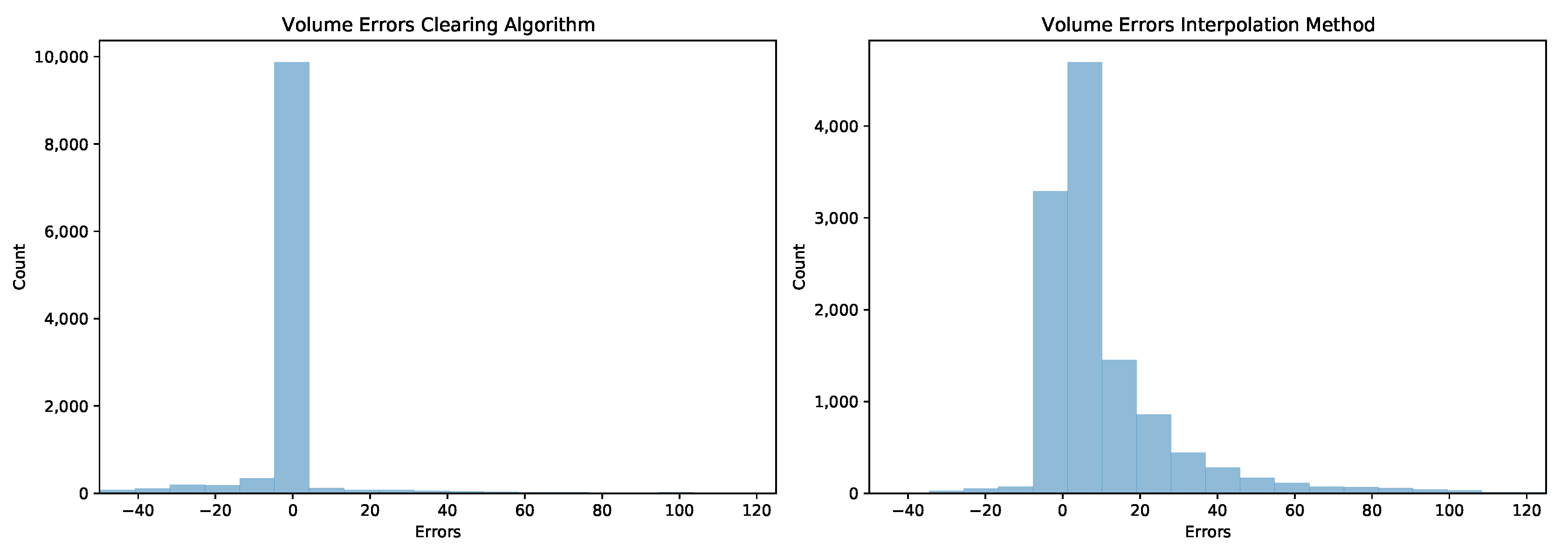
Next, we consider the estimates of the volumes. Although the volumes are of less interest, their accuracy should give confidence in the methods and help in deciding on which of the two methods to use. This time, the clearance algorithm gives the smallest errors on average, but also tends to underestimate the value. In contrast, the interpolation algorithm tends to overestimate the value. More details are shown in the histogram in Figure A2.
Figure A2.
Histogram for the clearing volumes for the clearing algorithm (left) and the interpolation method (right).
Figure A2.
Histogram for the clearing volumes for the clearing algorithm (left) and the interpolation method (right).

Given the analysis above, the decision was made to use the interpolation method. This was for several reasons. Firstly, although the clearance volume is more accurately predicted by the clearance method, the most important variable is the clearance price, which is much more accurately predicted using the interpolation method. Secondly, the interpolation method is much easier to implement than the clearance method.
Appendix A.2. X-Model
This section briefly describes the X-model [1] that was used as the basis for one of the core probabilistic day-ahead electricity price forecasting models presented in this report.
The model is split into several components:
- Deriving the clearance price from the supply and demand curves—this will be used as the actual price, as described in Appendix A.1.
- Deriving the price class time series from the supply and demand curves.
- Producing forecast models for each price class.
- Reconstructing the supply and demand curves from the price class forecast.
- Estimating the price from the intersection of the reconstructed supply and demand curves—this uses the same method to derive the clearance price and is described in Appendix A.1.
- Producing a probabilistic forecast from a residual bootstrap.
Each of the steps is elaborated upon in the individual sections below. The notation used throughout will be similar to that used in [1].
Appendix A.2.1. Producing Day-ahead Forecasts for Each Price Class
The model is only trained once for simplicity and to reduce the computational cost. This can be updated in future work. To model day d and hour h, the main variables for the model are denoted as follows:
where and are the volumes within each price classes at hour h for the supply and demand, respectively, where the price classes were defined in Section 3.1.1. Additionally included is the price and volume , (found from the intersection of the original supply and demand curves) and the offshore wind, onshore wind, and solar generation forecasts, , , and .
The dimension of for each hour and day is , where are the numbers of price classes for the supply and demand, respectively, and is the number of other variables. Note that only the first variables are to be forecast for each hour h of the next day. At present, the forecast is made from midnight of the day before. This is not strictly accurate, but is likely to make little difference in the forecast results. This should be considered in future work.
The first step is to reduce the data to a zero-mean time series , where is estimated using the sample mean. Further, since the LASSO model is a regularised least squares method, each variable is normalised to have unit variance. This assists with the training of the weights.
A linear model is considered for each hour, and is given by
with parameters and for the autoregressive coefficients and the day-of-the-week-effect coefficients, respectively. The day-of-the-week dummy variable is equal to one if k is equal to the same day of the week as d, and zero otherwise. The errors are assumed to be independent and identically distributed across days with constant variance .
A large number of lags are considered for the price components, and they are defined by
These represent the maximum size of the lags for different input variables. If the variable is the same class, then 36 days of lags are used for the same hour of the day, whereas only 8 days of lags are used if it is a different class but the same hour of the day, or the same class but a different hour. If the hour and class are different, only data from one day of lags are used.
The coefficients are found via a LASSO approach, which not only trains the variables, but also selects the best variables. Suppose that there is a linear model (written in matrix form for simplicity):
with a parameter vector
and a -dim vector of regressors:
The LASSO estimator is
with penalty ( means that there is no penalty on the number of variables, and hence, this is likely to lead to overfitting). If the penalty is too large, then the coefficients will simply be set to zero. The best penalty is found by maximising the Bayesian Information Criterion by implementing the least-angle regression implementation of LASSO, a very quick method for solving a highly parameterised LASSO optimisation.
Once the parameters are found, they can be rescaled to apply to the mean zero series and then re-centred to give the forecast for the original time series.
Appendix A.2.2. Reconstructing the Full Supply and Demand Curves
The forecasts produced are just for the price classes chosen by the method described in Section 3.1.1. To produce a price forecast, the supply and demand curves must be reconstructed, and then the wholesale price is simply the intersection of these curves. This is done on a price grid with 0.1 GBP increments, as in the X-model paper (but in GBP rather than EUR). This is slightly complicated, as a choice needs to be made regarding how the volumes from the price class will be distributed to the higher-resolution price grid.
The choice is made by looking at the historical data and calculating the most frequent probability that a volume is bid upon at each price level (rounded to the nearest 0.1 in our case), i.e., counting the proportion of bids made at price P. These are denoted and for the supply and demand, respectively (note that they are independent of the time period). The reconstructed volumes for supply and demand for hour h and day d are then given by
and
where and are the average volume curves for supply and demand, respectively, and are the current volumes forecast for price class c for hour h and day d for supply and demand, respectively, and and are Bernoulli random variables for supply and demand, respectively, with the associated probabilities generated from the available sample of historical data (although, as mentioned before, the combined training and test datasets are used instead due to the relatively small amount of data—this is not expected to change the results too dramatically, as the probabilities are likely to be similar).
The reconstruction probabilities (i.e., the Bernoulli random variables) are assumed to be independent in each price and also from the errors, , in the LASSO fit. This will enable a simple construction of the bootstrap forecasts (see Appendix A.2.3).
The way that the Bernoulli random variables are selected is dependent on whether a point or probabilistic model is being chosen.
- If a point forecast is being generated, then the value is set to if . In other words, if a price is seen, on average, twice a day, then it is included in the reconstruction. A similar process is used for the reconstruction of the demand curve. This is the same threshold as that used in [1].
- If considering a probabilistic forecast, then, instead of a fixed threshold as with the point forecast, for each bootstrapped price class forecast (see Appendix A.2.3), the supply and demand curves will be reconstructed by sampling from the Bernoulli distributions with their prescribed probabilities.
Once the supply and demand forecast curves have been reconstructed, then the forecast price is given by the intersection using the interpolation method described in Appendix A.1.
Appendix A.2.3. Probabilistic Forecast Generation
This section describes how a probabilistic forecast is created. Given the parameters found from the LASSO model (Appendix A.2.1), a point forecast for each normalised class time series is generated. Then, the sample means are re-added to obtain the bid volume forecasts for the following day.
A basic method for modelling the uncertainty around the forecast is produced by a residual bootstrap [1] from the training data. In other words, the residuals , which are the difference between the values from the model and the actual values in the training data, are randomly sampled with replacements and added to the current forecast vector to model the expected deviations from the mean. This can be repeated to produce B bootstrapped samples, with for for each price class. Then, the bootstrapped classes are reconstructed as supply and demand curves using the Bernoulli sampling method in Appendix A.2.2. The intersection of the supply and demand curves is then calculated for each bootstrap pair by using the interpolation method described in Appendix A.1. Note that the independent bootstrapping and Bernoulli random sampling are valid, since the price probabilities and the residual errors are assumed to be uncorrelated.
An adjustment to the simple bootstrap that randomly samples from the set of residuals for the entire training set but takes into account the correlation structure of the residuals is used instead. Let be a vector of residuals for day d and hour h for each of the price classes. Then, a daily residual vector can be defined as . The bootstrap is made from (i.e., from the n historical days) and is then applied to the current time series. This ensures that the correlation between price classes and the daily residual correlations are included in the model.
Appendix B. Extra Results
This appendix contains some extra results that did not fit within the main content of the paper, and these are given here as supporting material.
Appendix B.1. Price Class Forecasts
Figure A3 and Figure A4 show some day-ahead price class forecasts for the first two months of the test set for selected demand and supply classes, respectively. It is clear that some are more regular than others and are, hence, likely to be easier to accurately forecast.
Figure A3.
Examples of day-ahead forecasts for several classes for demand. The forecasts are in red and the actuals in black.
Figure A3.
Examples of day-ahead forecasts for several classes for demand. The forecasts are in red and the actuals in black.

Figure A4.
Day-ahead forecasts for selected supply classes in the test set. The forecasts are in red and the actual values are in black.
Figure A4.
Day-ahead forecasts for selected supply classes in the test set. The forecasts are in red and the actual values are in black.

Appendix B.2. Probability Integral Transforms
In Section 6.2, some probability integral transforms are presented for the first two months of the test set. For completeness, the PIT for the entire test set is given here for each of the main models. These are given in Figure A5, Figure A6 and Figure A7. Additionally note that the level for a uniform PIT is given in red, and this shows how the PIT would be distributed if the models were well calibrated over the entire test set.
In this case, unlike with the first two months, it is clear that the ARX model and X-model are both biased [28]. This means that the quantiles for these models are shifted too high for the observations. This is easily explained by the drift of the models, as seen in Figure 14 for the later months of the test set. As shown for the shorter test set, this bias is moved (in fact, it shifts to the other side) from the PIT. The bias is worse for the X-model, and this could be due to the accumulation of the forecast bias for each class. One way to reduce the bias in the ARX model and X-model would be to retain them at regular intervals. Other methods that have less bias than the LASSO model used here should be considered.
Figure A5.
PIT for the X-model for the entire test set.
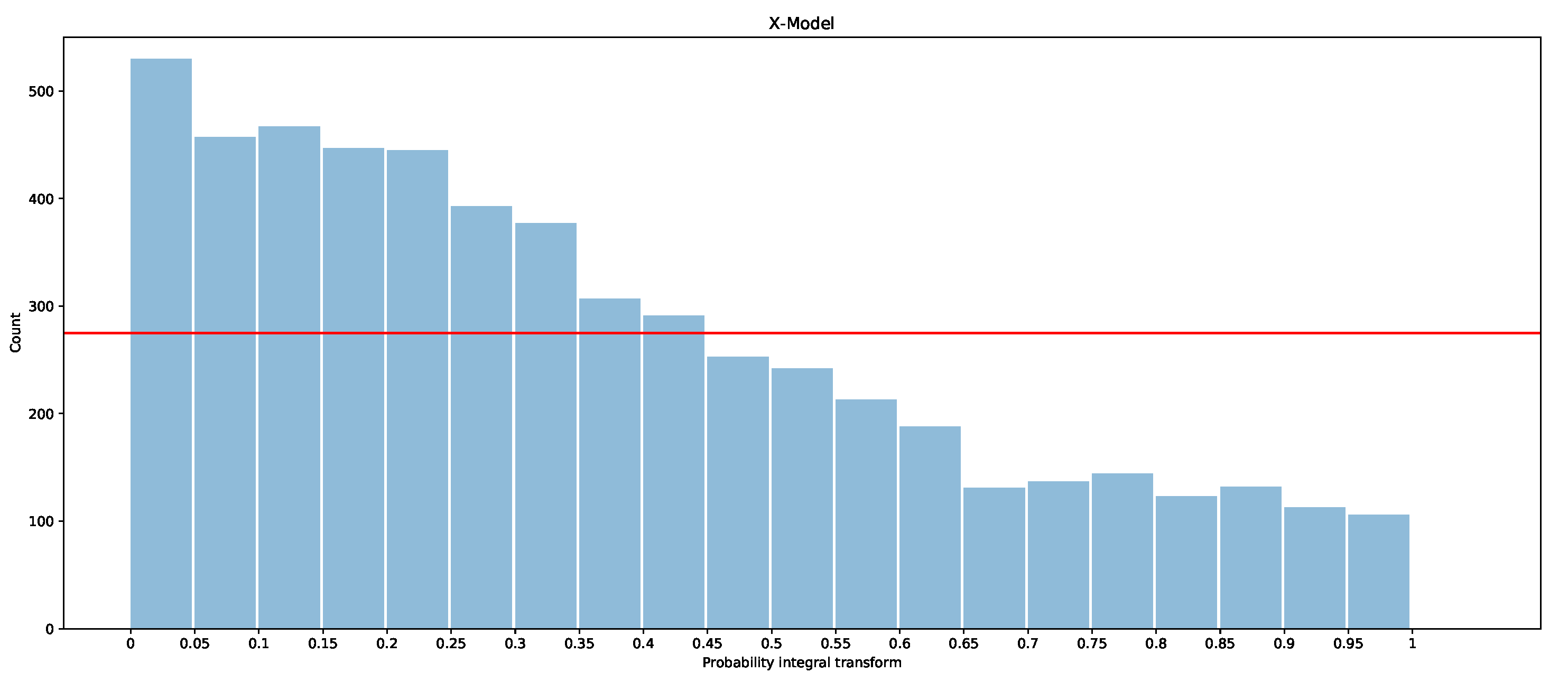
Figure A6.
PIT for the ARX model for the entire test set.

For the ARIMAX model, the PIT in Figure A7 shows an over-dispersion, which means that the quantiles are perhaps too wide for the actual underlying distribution. The underlying model for this method is a Gaussian distribution, which is clearly too wide, at least for this larger test set. As before, this is reduced in the shorter test set of two months, as shown in Figure 19, which is now more uniform, but has a slight bias.
Figure A7.
PIT for the ARIMAX model for the entire test set.

References
- Ziel, F.; Steinert, R. Electricity price forecasting using sale and purchase curves: The x-model. Energy Econ. 2016, 59, 435–454. [Google Scholar] [CrossRef] [Green Version]
- Weron, R. Electricity price forecasting: A review of the state-of-the-art with a look into the future. Int. J. Forecast. 2014, 30, 1030–1081. [Google Scholar] [CrossRef] [Green Version]
- Nowotarski, J.; Weron, R. Recent advances in electricity price forecasting: A review of probabilistic forecasting. Renew. Sustain. Energy Rev. 2018, 81, 1548–1568. [Google Scholar] [CrossRef]
- Lago, J.; Marcjasz, G.; De Schutter, B.; Weron, R. Forecasting day-ahead electricity prices: A review of state-of-the-art algorithms, best practices and an open-access benchmark. Appl. Energy 2021, 293, 116983. [Google Scholar] [CrossRef]
- Maciejowska, K.; Nowotarski, J.; Weron, R. Probabilistic forecasting of electricity spot prices using Factor Quantile Regression Averaging. Int. J. Forecast. 2016, 32, 957–965. [Google Scholar] [CrossRef]
- Efron, B.; Tibshirani, R.J. An Introduction to the Bootstrap; Chapman & Hall: New York, NY, USA, 1993. [Google Scholar]
- Clements, M.P.; Kim, J.H. Bootstrap prediction intervals for autoregressive time series. Comput. Stat. Data Anal. 2007, 51, 3580–3594. [Google Scholar] [CrossRef]
- Nowotarski, J.; Weron, R. Computing electricity spot price prediction intervals using quantile regression and forecast averaging. Comput. Stat. 2015, 30, 791–803. [Google Scholar] [CrossRef] [Green Version]
- Maciejowska, K.; Nowotarski, J. A hybrid model for GEFCom2014 probabilistic electricity price forecasting. Int. J. Forecast. 2016, 32, 1051–1056. [Google Scholar] [CrossRef] [Green Version]
- Gaillard, P.; Goude, Y.; Nedellec, R. Additive models and robust aggregation for GEFCom2014 probabilistic electric load and electricity price forecasting. Int. J. Forecast. 2016, 32, 1038–1050. [Google Scholar] [CrossRef]
- Uniejewski, B.; Weron, R. Regularized quantile regression averaging for probabilistic electricity price forecasting. Energy Econ. 2021, 95, 105121. [Google Scholar] [CrossRef]
- Banitalebi, B.; Hoque, M.E.; Appadoo, S.S.; Thavaneswaran, A. Regularized Probabilistic Forecasting of Electricity Wholesale Price and Demand. In Proceedings of the 2020 IEEE Symposium Series on Computational Intelligence (SSCI), Canberra, Australia, 1–4 December 2020; pp. 28–35. [Google Scholar]
- He, H.; Lu, N.; Jiang, Y.; Chen, B.; Jiao, R. End-to-end probabilistic forecasting of electricity price via convolutional neural network and label distribution learning. Energy Rep. 2020, 6, 1176–1183. [Google Scholar] [CrossRef]
- Brusaferri, A.; Matteucci, M.; Portolani, P.; Vitali, A. Bayesian deep learning based method for probabilistic forecast of day-ahead electricity prices. Appl. Energy 2019, 250, 1158–1175. [Google Scholar] [CrossRef]
- Marcjasz, G.; Uniejewski, B.; Weron, R. Probabilistic electricity price forecasting with NARX networks: Combine point or probabilistic forecasts? Int. J. Forecast. 2020, 36, 466–479. [Google Scholar] [CrossRef]
- Uniejewski, B.; Marcjasz, G.; Weron, R. On the importance of the long-term seasonal component in day-ahead electricity price forecasting: Part II—Probabilistic forecasting. Energy Econ. 2019, 79, 171–182. [Google Scholar] [CrossRef] [Green Version]
- Bernardi, M.; Lisi, F. Point and Interval Forecasting of Zonal Electricity Prices and Demand Using Heteroscedastic Models: The IPEX Case. Energies 2020, 13, 6191. [Google Scholar] [CrossRef]
- Mehmood, N.; Arshad, N. Interval Forecasting of Hourly Electricity Spot Prices using Rolling Window Based Gaussian Process Regression. In Proceedings of the 2020 2nd International Conference on Smart Power & Internet Energy Systems (SPIES), Bangkok, Thailand, 15–18 September 2020; pp. 469–473. [Google Scholar]
- Taylor, J.W. Evaluating quantile-bounded and expectile-bounded interval forecasts. Int. J. Forecast. 2021, 37, 800–811. [Google Scholar] [CrossRef]
- Kath, C.; Ziel, F. Conformal prediction interval estimation and applications to day-ahead and intraday power markets. Int. J. Forecast. 2021, 37, 777–799. [Google Scholar] [CrossRef]
- Christensen, T.; Hurn, A.; Lindsay, K. Forecasting spikes in electricity prices. Int. J. Forecast. 2012, 28, 400–411. [Google Scholar] [CrossRef]
- Bello, A.; Reneses, J.; Muñoz, A. Medium-term probabilistic forecasting of extremely low prices in electricity markets: Application to the Spanish case. Energies 2016, 9, 193. [Google Scholar] [CrossRef]
- Zareipour, H.; Janjani, A.; Leung, H.; Motamedi, A.; Schellenberg, A. Classification of future electricity market prices. IEEE Trans. Power Syst. 2011, 26, 165–173. [Google Scholar] [CrossRef]
- Haben, S.; Ward, J.; Greetham, D.; Grindrod, P.; Singleton, C. A New Error Measure for Forecasts of Household-level, High Resolution Electrical Energy Consumption. Int. J. Forecast. 2014, 30, 246–256. [Google Scholar] [CrossRef] [Green Version]
- Gneiting, T.; Raftery, A. Strictly Proper Scoring Rules, Prediction, and Estimation. J. Am. Stat. Assoc. 2007, 102, 477. [Google Scholar] [CrossRef]
- Hong, T.; Pinson, P.; Fan, S.; Zareipour, H.; Troccoli, A.; Hyndman, R.J. Probabilistic energy forecasting: Global Energy Forecasting Competition 2014 and beyond. Int. J. Forecast. 2016, 32, 896–913. [Google Scholar] [CrossRef] [Green Version]
- Ziel, F.; Steinert, R. Probabilistic mid- and long-term electricity price forecasting. Renew. Sustain. Energy Rev. 2018, 94, 251–266. [Google Scholar] [CrossRef] [Green Version]
- Polsterer, K.; D’Isanto, A.; Gieseke, F. Uncertain Photometric Redshifts; Annual Meeting of the German Astronomical Sociery: Bochum, Germany, 2016. [Google Scholar]
- EPEX SPOT SE (2020a). Annual Report 2019. Available online: https://www.epexspot.com/sites/default/files/downloadcenterfiles/Epex-spot-2019200703Planche.pdf (accessed on 10 August 2021).
- Energy Systems Catapult. The Policy and Regulatory Context for New Local Energy Markets. 2019. Available online: https://es.catapult.org.uk/reports/the-policy-and-regulatory-context-for-new-local-energy-markets/ (accessed on 10 August 2021).
Figure 1.
Example of the supply (blue) and demand (orange) curves and their intersection (blue dot) giving the wholesale clearance price.
Figure 1.
Example of the supply (blue) and demand (orange) curves and their intersection (blue dot) giving the wholesale clearance price.
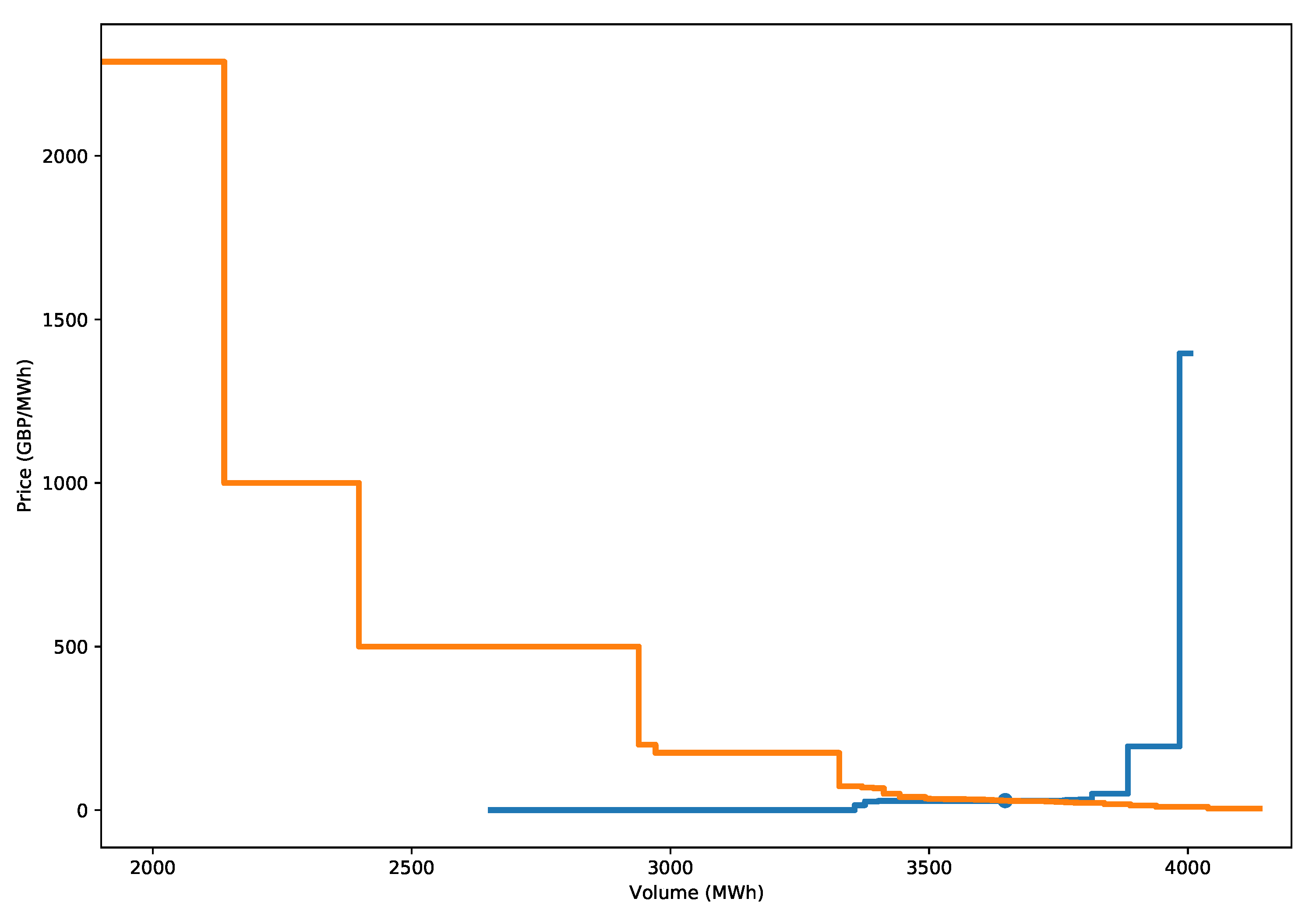
Figure 2.
Illustration of price classes for the supply (left) and demand curves (right).
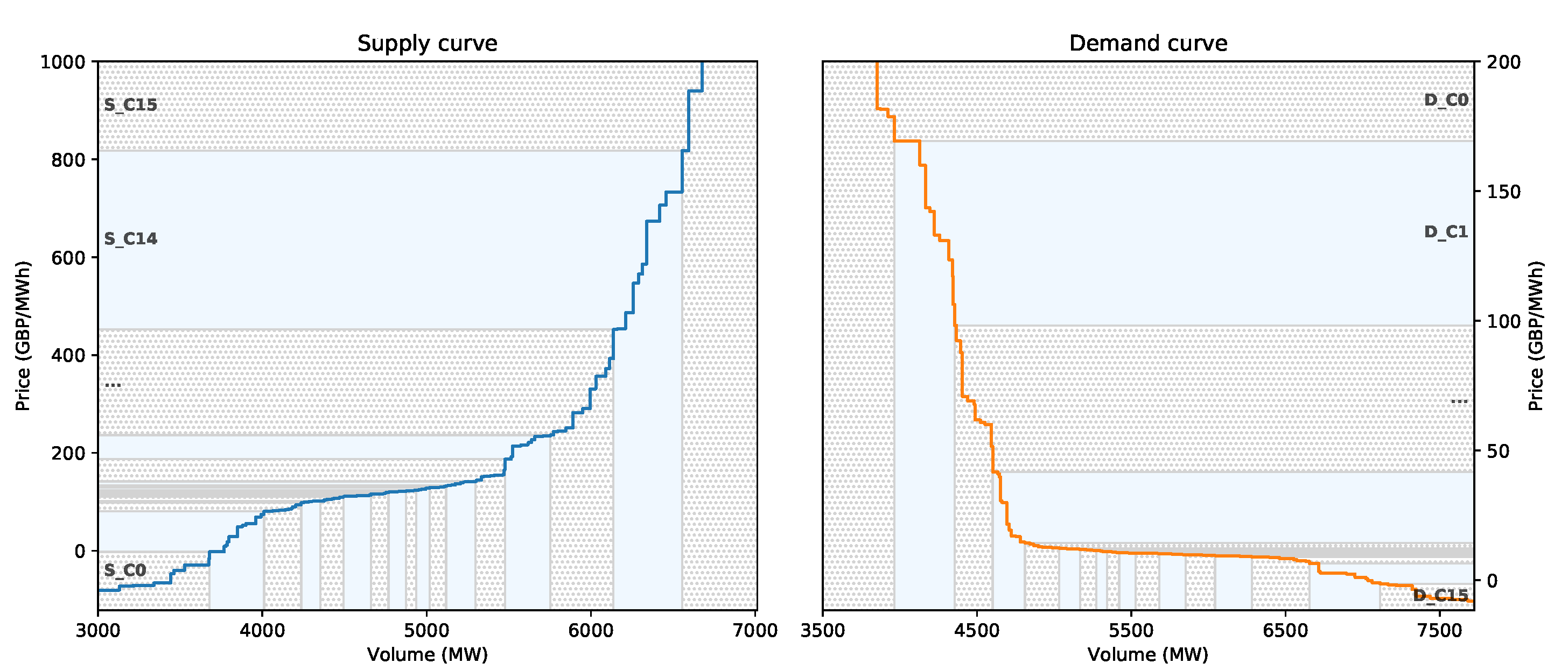
Figure 3.
Estimates of the clearing price for the period 11 April 2018 to 17 August 2019.

Figure 4.
Estimates of the clearing volumes (in MWh) for the period 11 April 2018 to 17 August 2019.
Figure 4.
Estimates of the clearing volumes (in MWh) for the period 11 April 2018 to 17 August 2019.

Figure 5.
Day-ahead forecasts for the solar (top), offshore wind (middle), and onshore generation (bottom) for the period of 11 April 2018 to 17 August 2019.
Figure 5.
Day-ahead forecasts for the solar (top), offshore wind (middle), and onshore generation (bottom) for the period of 11 April 2018 to 17 August 2019.
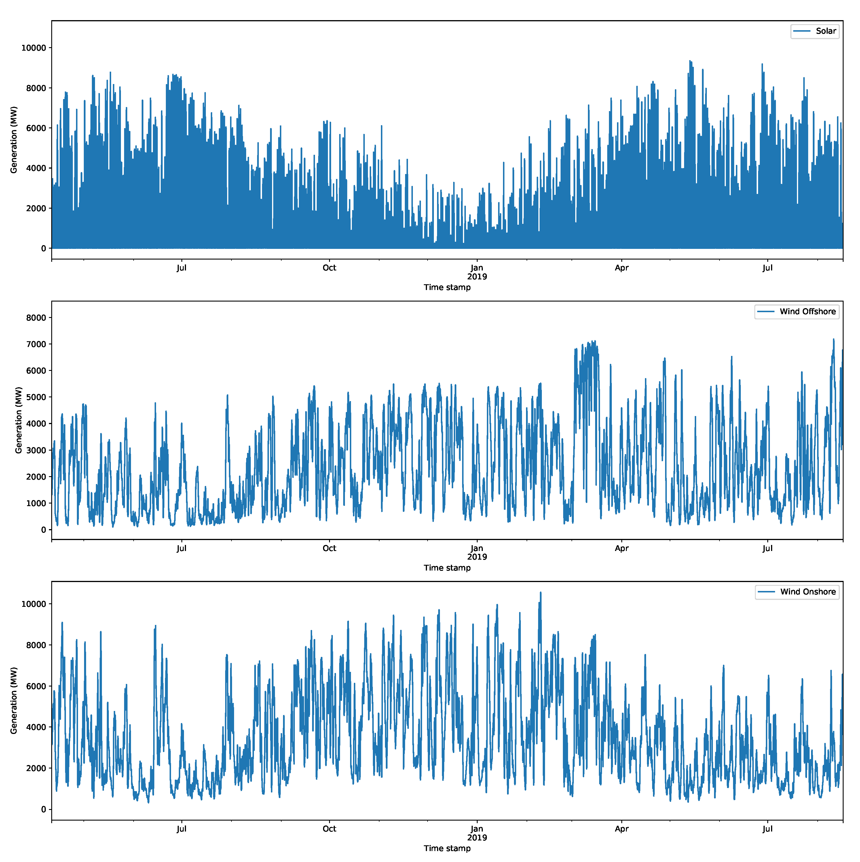
Figure 6.
Sample of the volume time series for the first class, D_C0, for the demand.

Figure 7.
Samples of the volume time series for other demand classes.

Figure 8.
Autocorrelation and partial autocorrelation for the first demand class, D_C0.

Figure 9.
Sample of the volume time series for the first supply class.

Figure 10.
Selected classes for the supply volume time series.
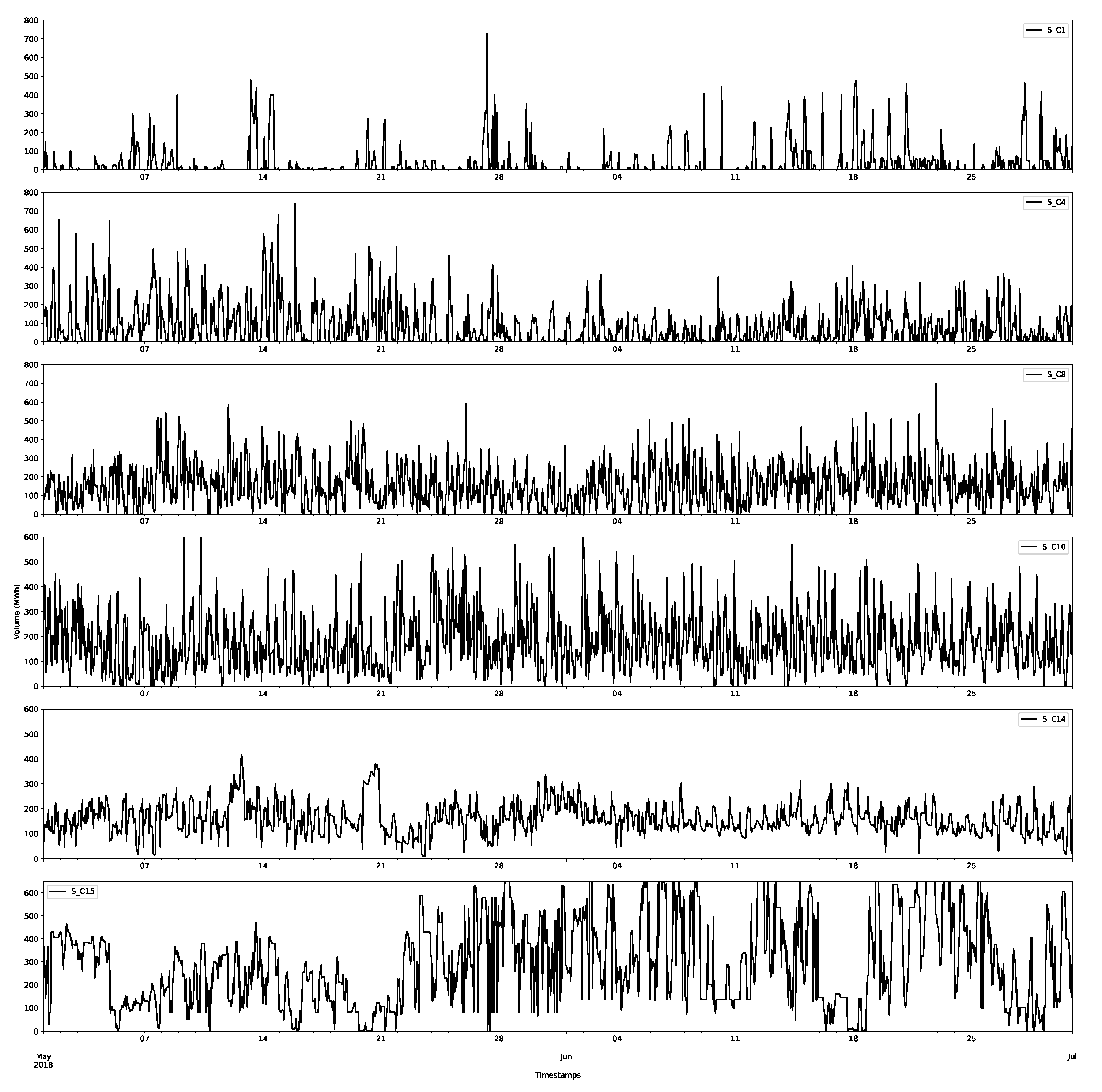
Figure 11.
Example of day-ahead forecasting for the first demand class for the first two months of the test set. The actual values are in black and the forecast values are in red.
Figure 11.
Example of day-ahead forecasting for the first demand class for the first two months of the test set. The actual values are in black and the forecast values are in red.

Figure 12.
Day-ahead forecast for the first supply class for the first two months of the test set. The actual values are in black and the forecast values are in red.
Figure 12.
Day-ahead forecast for the first supply class for the first two months of the test set. The actual values are in black and the forecast values are in red.

Figure 13.
Example of the X-model’s and ARX model’s rolling day-ahead point forecasts for the first month of the test set. Black is the actual, red is the X-model forecast, and blue is the ARX model forecast.
Figure 13.
Example of the X-model’s and ARX model’s rolling day-ahead point forecasts for the first month of the test set. Black is the actual, red is the X-model forecast, and blue is the ARX model forecast.

Figure 14.
Example of the day-ahead price forecasts of the X-model’s (red) and the ARX model’s point forecasts (blue) for one of the later months of the testing set (May 2019). This was obtained using the training data from 1 January 2017 to 1 January 2019.
Figure 14.
Example of the day-ahead price forecasts of the X-model’s (red) and the ARX model’s point forecasts (blue) for one of the later months of the testing set (May 2019). This was obtained using the training data from 1 January 2017 to 1 January 2019.

Figure 15.
Reconstructed day-ahead forecasts for prices with the fixed threshold method (i.e., the point forecast in blue) and two Bernoulli random draws (red) for selected days in the test set. These are compared to the actual prices (black).
Figure 15.
Reconstructed day-ahead forecasts for prices with the fixed threshold method (i.e., the point forecast in blue) and two Bernoulli random draws (red) for selected days in the test set. These are compared to the actual prices (black).

Figure 16.
Sample of the ARIMAX model’s forecast for the first nine days of the test set. The different confidence bounds are given different shades, with the darkest representing the prediction interval for the middle ten percent. The actual prices are given by the black line.
Figure 16.
Sample of the ARIMAX model’s forecast for the first nine days of the test set. The different confidence bounds are given different shades, with the darkest representing the prediction interval for the middle ten percent. The actual prices are given by the black line.

Figure 17.
Sample of the ARX model’s forecast for the first nine days of the test period. The different confidence bounds are given different shades, with the darkest representing the prediction interval for the middle ten percent. The actual prices are given by the black line.
Figure 17.
Sample of the ARX model’s forecast for the first nine days of the test period. The different confidence bounds are given different shades, with the darkest representing the prediction interval for the middle ten percent. The actual prices are given by the black line.
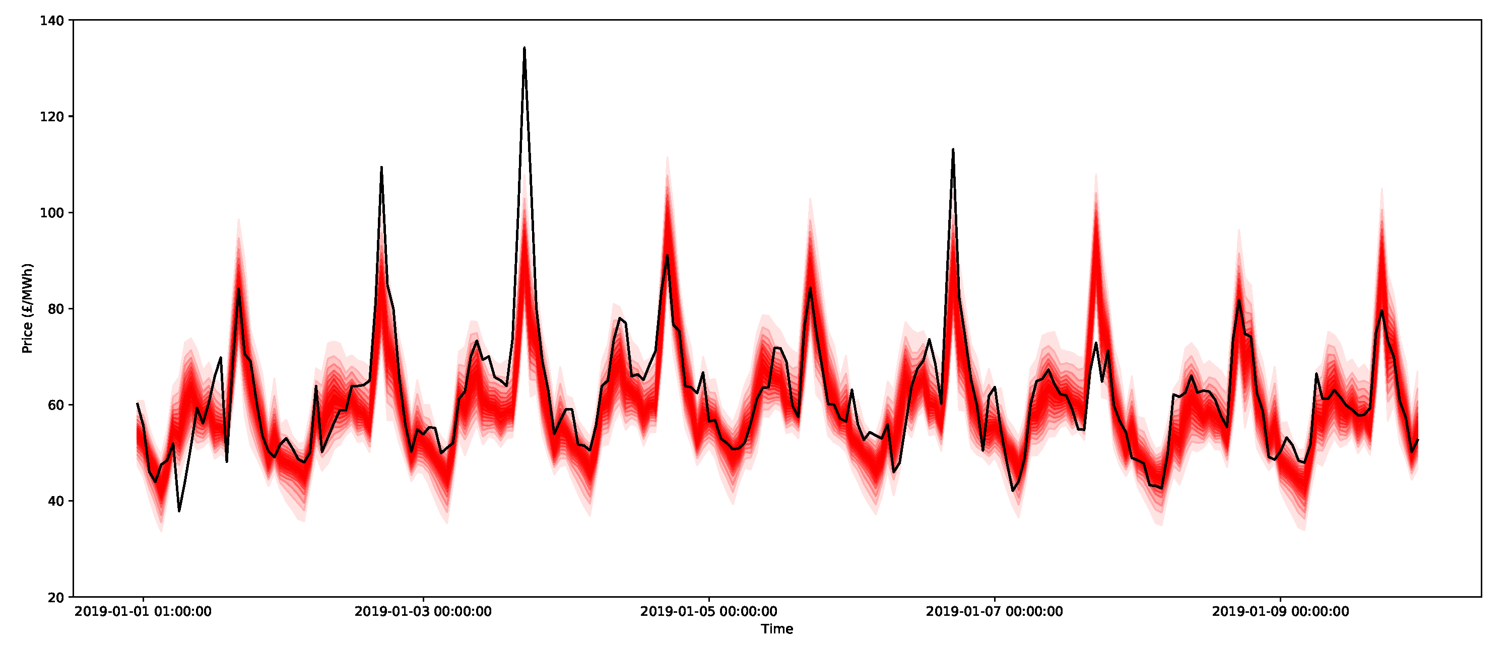
Figure 18.
Sample of the X-model’s forecast for the first nine days of the test periods. The different confidence bounds are given different shades, with the darkest representing the prediction interval for the middle ten percent. The actual prices are given by the black line.
Figure 18.
Sample of the X-model’s forecast for the first nine days of the test periods. The different confidence bounds are given different shades, with the darkest representing the prediction interval for the middle ten percent. The actual prices are given by the black line.

Figure 19.
PIT for the ARIMAX model for the first two months of the test set.

Figure 20.
PIT for the ARX model for the first two months of the test set.

Figure 21.
PIT for the X-model for the first two months of the test set.

Figure 22.
Example of 50 ensembles (red) for the ARX method for the first day of the test set. The actual price is in black.
Figure 22.
Example of 50 ensembles (red) for the ARX method for the first day of the test set. The actual price is in black.

Figure 23.
Example of 50 ensembles (blue) for the X-model method for the first day of the test set. The actual price is in black.
Figure 23.
Example of 50 ensembles (blue) for the X-model method for the first day of the test set. The actual price is in black.
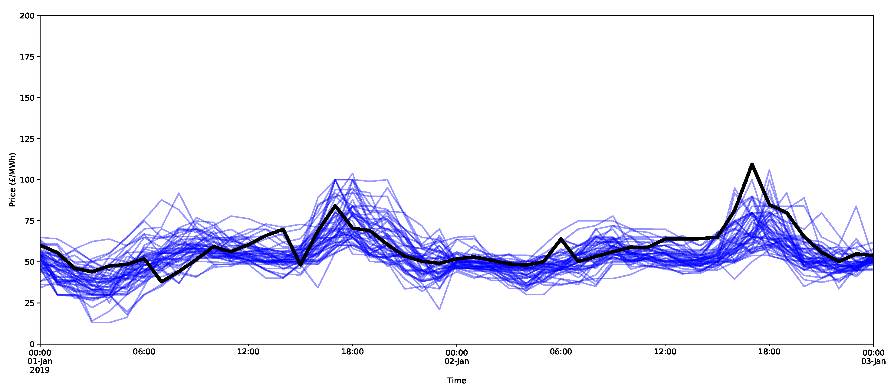
Figure 24.
Quantile estimates (red) for 3 January 2019 for each of the forecast models. The actual is shown in black.
Figure 24.
Quantile estimates (red) for 3 January 2019 for each of the forecast models. The actual is shown in black.

Figure 25.
All 2000 bootstrap ensembles (red) for the ARX method for 3 January 2019. The true price is in black.
Figure 25.
All 2000 bootstrap ensembles (red) for the ARX method for 3 January 2019. The true price is in black.

Figure 26.
All 2000 bootstrap ensembles (blue) for the X-model method for 3 January 2019. The true price is in black.
Figure 26.
All 2000 bootstrap ensembles (blue) for the X-model method for 3 January 2019. The true price is in black.

Figure 27.
Supply and demand curves for the hours around the peak price on 3 January 2019. The demand curves are in blue and the supply curves are in orange.
Figure 27.
Supply and demand curves for the hours around the peak price on 3 January 2019. The demand curves are in blue and the supply curves are in orange.
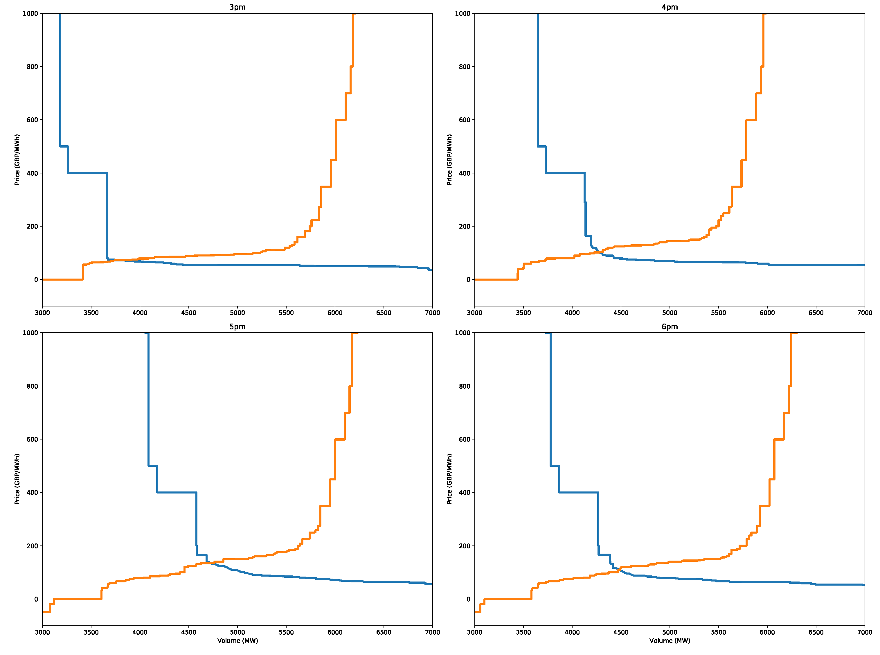
Table 1.
Average RMSE score of each method over the entire test set.
| Method | RMSE |
|---|---|
| Daily Persistence | 7.61 |
| ARX Benchmark | 6.13 |
| X-Model | 9.51 |
| ARIMAX | 6.03 |
Table 2.
Average RMSE scores for each method per test month. The best scores per month are in bold.
| RMSE | Jan 19 | Feb 19 | Mar 19 | Apr 19 | May 19 | Jun 19 | Jul 19 |
|---|---|---|---|---|---|---|---|
| Persistence | 10.6 | 7.1 | 8.4 | 6.3 | 6.4 | 7.9 | 5.8 |
| ARX | 8.11 | 5.15 | 6.18 | 5.42 | 5.54 | 6.59 | 4.97 |
| ARIMAX | 8.46 | 6.01 | 6.11 | 5.32 | 4.90 | 6.38 | 4.54 |
| X-Model | 10.65 | 6.72 | 8.90 | 8.56 | 9.40 | 11.64 | 8.88 |
Table 3.
Average pinball scores for the three main methods. The best-scoring method is shown in bold.
Table 3.
Average pinball scores for the three main methods. The best-scoring method is shown in bold.
| Model | Average Pinball Score |
|---|---|
| ARIMAX | 1.72 |
| ARX Model | 1.71 |
| X-Model | 2.59 |
Table 4.
Monthly average pinball score for each method. In bold is the best-scoring method for each month.
Table 4.
Monthly average pinball score for each method. In bold is the best-scoring method for each month.
| Pinball Scores | Jan 19 | Feb 19 | Mar 19 | Apr 19 | May 19 | Jun 19 | Jul 19 |
|---|---|---|---|---|---|---|---|
| ARIMAX | 2.32 | 1.77 | 1.79 | 1.59 | 1.48 | 1.79 | 1.40 |
| ARX | 2.20 | 1.47 | 1.76 | 1.56 | 1.56 | 1.85 | 1.41 |
| X-Model | 2.95 | 1.93 | 2.45 | 2.35 | 2.54 | 3.23 | 2.36 |
Table 5.
Pinball scores for the peak hours on 3 January 2019 for the three forecast models. In bold are the best scores for that time period.
Table 5.
Pinball scores for the peak hours on 3 January 2019 for the three forecast models. In bold are the best scores for that time period.
| Time Period on 3 Jan | Pinball Score | ||
|---|---|---|---|
| X-Model | ARX | ARIMAX | |
| 2pm | 4.02 | 1.72 | 0.87 |
| 3pm | 5.55 | 5.78 | 4.04 |
| 4pm | 14.18 | 11.78 | 9.46 |
| 5pm | 26.46 | 19.03 | 18.55 |
| 6pm | 12.68 | 14.15 | 12.61 |
| 7pm | 4.94 | 2.27 | 1.71 |
| 8pm | 4.84 | 1.73 | 0.99 |
Publisher’s Note: MDPI stays neutral with regard to jurisdictional claims in published maps and institutional affiliations. |
© 2021 by the authors. Licensee MDPI, Basel, Switzerland. This article is an open access article distributed under the terms and conditions of the Creative Commons Attribution (CC BY) license (https://creativecommons.org/licenses/by/4.0/).
Share and Cite
MDPI and ACS Style
Haben, S.; Caudron, J.; Verma, J. Probabilistic Day-Ahead Wholesale Price Forecast: A Case Study in Great Britain. Forecasting 2021, 3, 596-632. https://0-doi-org.brum.beds.ac.uk/10.3390/forecast3030038
AMA Style
Haben S, Caudron J, Verma J. Probabilistic Day-Ahead Wholesale Price Forecast: A Case Study in Great Britain. Forecasting. 2021; 3(3):596-632. https://0-doi-org.brum.beds.ac.uk/10.3390/forecast3030038
Chicago/Turabian StyleHaben, Stephen, Julien Caudron, and Jake Verma. 2021. "Probabilistic Day-Ahead Wholesale Price Forecast: A Case Study in Great Britain" Forecasting 3, no. 3: 596-632. https://0-doi-org.brum.beds.ac.uk/10.3390/forecast3030038