
Short Term Electric Power Load Forecasting Using Principal Component Analysis and Recurrent Neural Networks

 ,
,  , and
, and 
Abstract
:1. Introduction
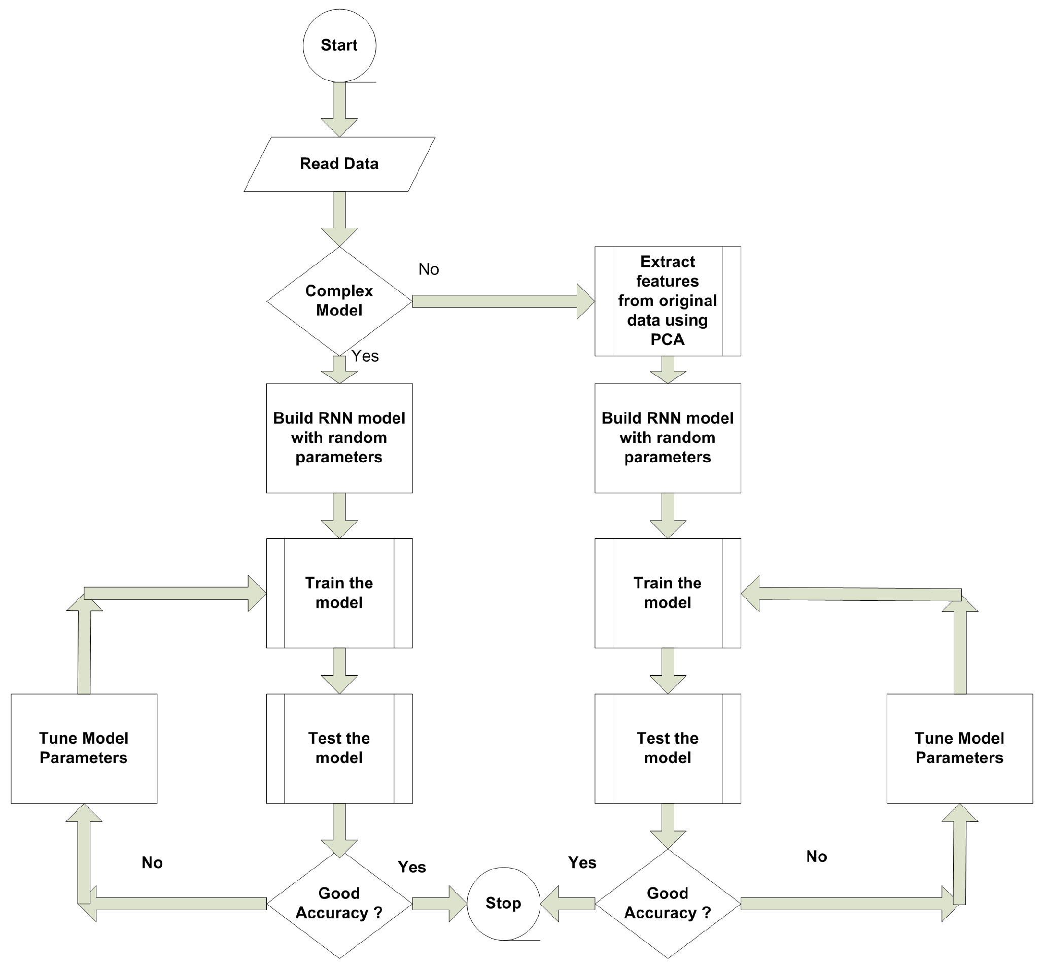
2. Methodology
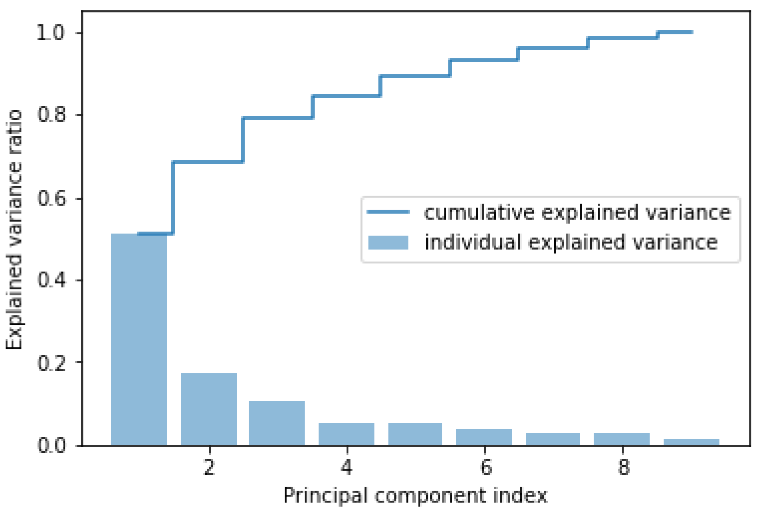
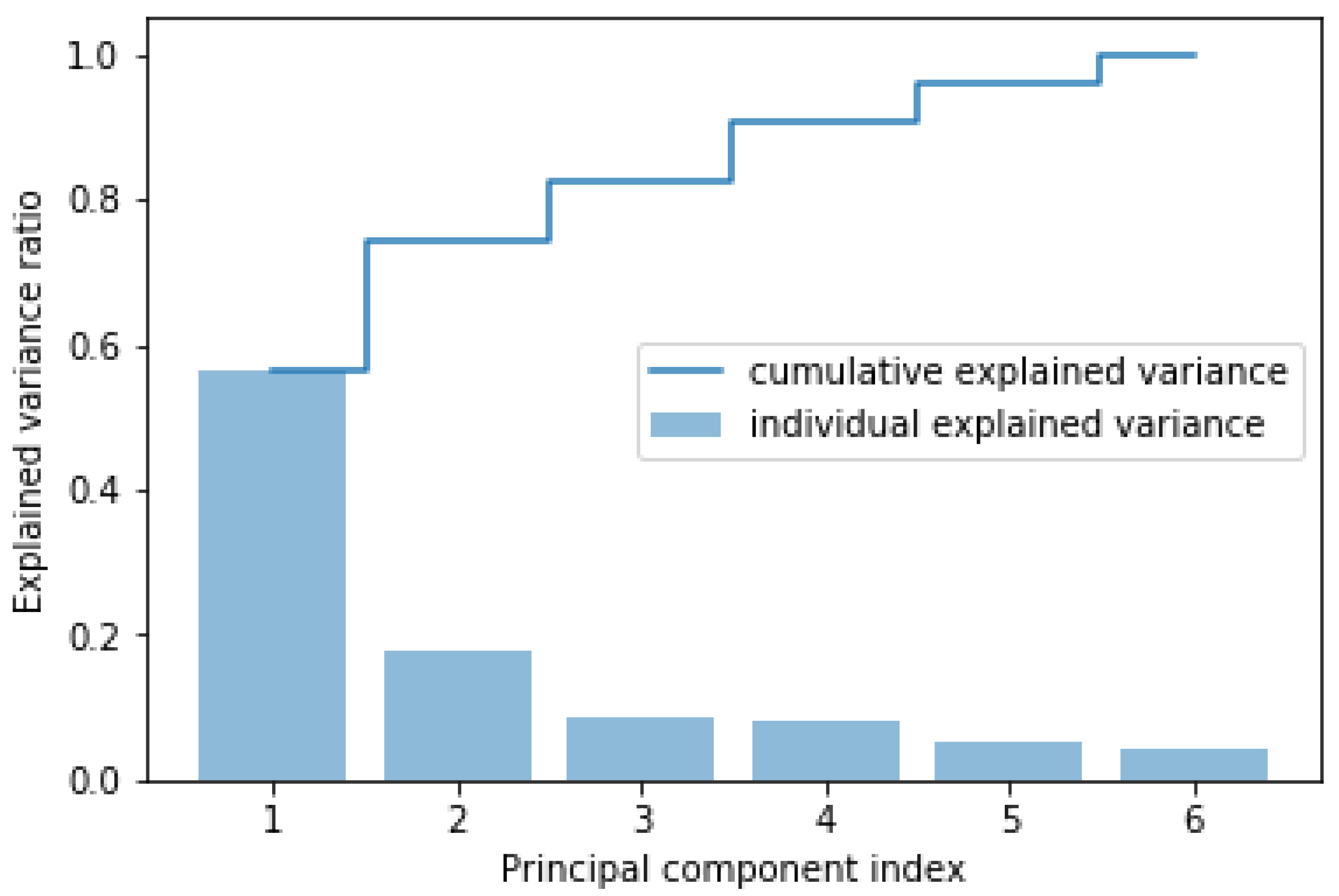
2.1. Dimensionality Reduction Using Principal Component Analysis (PCA)
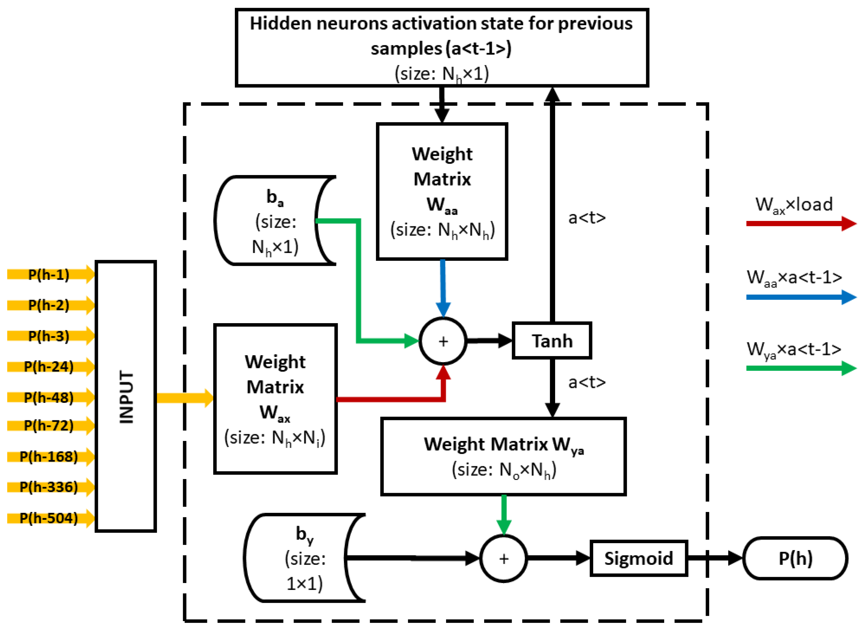
2.2. Recurrent Neural Network (RNN)
3. Result Analysis
3.1. Load Forecasting for HAM-(RHM-1)
3.2. Load Forecasting for HAM-(RHM-2)
3.3. Load Forecasting for DAM-(RDM-1)
3.4. Load Forecasting for DAM-(RDM-2)
3.5. Comparative Result Analysis
4. Conclusions
Author Contributions
Funding
Institutional Review Board Statement
Informed Consent Statement
Data Availability Statement
Acknowledgments
Conflicts of Interest
Abbreviations
| Load at hour | |
| Load at one hour before from the time of prediction | |
| Load at two hours before from the time of prediction | |
| Load at three hours before from time of prediction | |
| Load at one day before from the time of prediction | |
| Load at two days before from the time of prediction | |
| Load at three days before from time of prediction | |
| Load at one week before from the time of prediction | |
| Load at two weeks before from the time of prediction | |
| Load at three weeks before from time of prediction | |
| MSE | Mean Square Error |
| MAE | Mean Absolute Error |
| RMSE | Root Mean Square Error |
| a | Hidden neuron current activation state |
| a | Hidden neuron previous activation state |
| Bias parameter for hidden layer | |
| Bias parameter for output layer | |
| Weight matrix between input and hidden layer | |
| Weight matrix between output and hidden layer | |
| DAM | Day ahead market |
| HAM | Hourly ahead market |
| RHM-1 | Recurrent Neural Network Model for Hourly Ahead Market |
| RHM-2 | Light weight recurrent neural network Model for Hourly Ahead Market |
| RDM-1 | Recurrent Neural Network Model for day ahead market |
| RDM-2 | Light weight recurrent neural network Model for day ahead market |
| Actual load from sample | |
| Predicted load with sample |
References
- Ahmad, T.; Chen, H. A review on machine learning forecasting growth trends and their real-time applications in different energy systems. Sustain. Cities Soc. 2020, 54, 102010. [Google Scholar] [CrossRef]
- Akhavan-Hejazi, H.; Mohsenian-Rad, H. Power systems big data analytics: An assessment of paradigm shift barriers and prospects. Energy Rep. 2018, 4, 91–100. [Google Scholar] [CrossRef]
- Almeshaiei, E.; Soltan, H. A methodology for electric power load forecasting. Alex. Eng. J. 2011, 50, 137–144. [Google Scholar] [CrossRef] [Green Version]
- Khodayar, M.E.; Wu, H. Demand forecasting in the Smart Grid paradigm: Features and challenges. Electr. J. 2015, 28, 51–62. [Google Scholar] [CrossRef]
- Mansoor, M.; Grimaccia, F.; Leva, S.; Mussetta, M. Comparison of echo state network and feed-forward neural networks in electrical load forecasting for demand response programs. Math. Comput. Simul. 2021, 184, 282–293. [Google Scholar] [CrossRef]
- Su, P.; Tian, X.; Wang, Y.; Deng, S.; Zhao, J.; An, Q.; Wang, Y. Recent trends in load forecasting technology for the operation optimization of distributed energy system. Energies 2017, 10, 1303. [Google Scholar] [CrossRef] [Green Version]
- Zheng, X.; Ran, X.; Cai, M. Short-term load forecasting of power system based on neural network intelligent algorithm. IEEE Access 2020. [Google Scholar] [CrossRef]
- Vasudevan, S. One-Step-Ahead Load Forecasting for Smart Grid Applications. Ph.D. Thesis, The Ohio State University, Columbus, OH, USA, 2011. [Google Scholar]
- Neusser, L.; Canha, L.N. Real-time load forecasting for demand side management with only a few days of history available. In Proceedings of the 4th International Conference on Power Engineering, Energy and Electrical Drives, Istanbul, Turkey, 13–17 May 2013; pp. 911–914. [Google Scholar]
- Singh, A.K.; Khatoon, S.; Muazzam, M.; Chaturvedi, D.K. Load forecasting techniques and methodologies: A review. In Proceedings of the 2012 2nd International Conference on Power, Control and Embedded Systems, Allahabad, India, 17–19 December 2012; pp. 1–10.
- Ahmad, F.; Alam, M.S. Assessment of power exchange based electricity market in India. Energy Strategy Rev. 2019, 23, 163–177. [Google Scholar] [CrossRef]
- Massaoudi, M.; Refaat, S.S.; Chihi, I.; Trabelsi, M.; Oueslati, F.S.; Abu-Rub, H. A novel stacked generalization ensemble-based hybrid LGBM-XGB-MLP model for Short-Term Load Forecasting. Energy 2021, 214, 118874. [Google Scholar] [CrossRef]
- Yin, L.; Xie, J. Multi-temporal-spatial-scale temporal convolution network for short-term load forecasting of power systems. Appl. Energy 2021, 283, 116328. [Google Scholar] [CrossRef]
- Syed, D.; Abu-Rub, H.; Ghrayeb, A.; Refaat, S.S.; Houchati, M.; Bouhali, O.; Bañales, S. Deep learning-based short-term load forecasting approach in smart grid with clustering and consumption pattern recognition. IEEE Access 2021, 9, 54992–55008. [Google Scholar] [CrossRef]
- Munkhammar, J.; van der Meer, D.; Widén, J. Very short term load forecasting of residential electricity consumption using the Markov-chain mixture distribution (MCM) model. Appl. Energy 2021, 282, 116180. [Google Scholar] [CrossRef]
- Guo, W.; Che, L.; Shahidehpour, M.; Wan, X. Machine-Learning based methods in short-term load forecasting. Electr. J. 2021, 34, 106884. [Google Scholar] [CrossRef]
- Eskandari, H.; Imani, M.; Moghaddam, M.P. Convolutional and recurrent neural network based model for short-term load forecasting. Electr. Power Syst. Res. 2021, 195, 107173. [Google Scholar] [CrossRef]
- Sheng, Z.; Wang, H.; Chen, G.; Zhou, B.; Sun, J. Convolutional residual network to short-term load forecasting. Appl. Intell. 2021, 51, 2485–2499. [Google Scholar] [CrossRef]
- Veeramsetty, V.; Mohnot, A.; Singal, G.; Salkuti, S.R. Short Term Active Power Load Prediction on A 33/11 kV Substation Using Regression Models. Energies 2021, 14, 2981. [Google Scholar] [CrossRef]
- Veeramsetty, V.; Chandra, D.R.; Salkuti, S.R. Short-term electric power load forecasting using factor analysis and long short-term memory for smart cities. Int. J. Circuit Theory Appl. 2021, 49, 1678–1703. [Google Scholar] [CrossRef]
- Grimaccia, F.; Mussetta, M.; Zich, R. Neuro-fuzzy predictive model for PV energy production based on weather forecast. In Proceedings of the 2011 IEEE International Conference on Fuzzy Systems (FUZZ-IEEE 2011), Taipei, Taiwan, 27–30 June 2011; pp. 2454–2457. [Google Scholar] [CrossRef]
- Veeramsetty, V.; Deshmukh, R. Electric power load forecasting on a 33/11 kV substation using artificial neural networks. SN Appl. Sci. 2020, 2, 855. [Google Scholar] [CrossRef] [Green Version]
- Hong, T.; Pinson, P.; Fan, S.; Zareipour, H.; Troccoli, A.; Hyndman, R.J. Probabilistic energy forecasting: Global Energy Forecasting Competition 2014 and beyond. Int. J. Forecast. 2016, 32, 896–913. [Google Scholar] [CrossRef] [Green Version]
- Veeramsetty, V.; Reddy, K.R.; Santhosh, M.; Mohnot, A.; Singal, G. Short-term electric power load forecasting using random forest and gated recurrent unit. Electr. Eng. 2021, 1–23. [Google Scholar] [CrossRef]
- Abdi, H.; Williams, L.J. Principal component analysis. Wiley Interdiscip. Rev. Comput. Stat. 2010, 2, 433–459. [Google Scholar] [CrossRef]
- Mandic, D.P.; Chambers, J. Recurrent Neural Networks for Prediction: Learning Algorithms, Architectures and Stability; John Wiley & Sons, Inc.: Hoboken, NJ, USA, 2001. [Google Scholar]
- Karri, C.; Durgam, R.; Raghuram, K. Electricity Price Forecasting in Deregulated Power Markets using Wavelet-ANFIS-KHA. In Proceedings of the 2018 International Conference on Computing, Power and Communication Technologies (GUCON), Greater Noida, India, 28–29 September 2018; pp. 982–987. [Google Scholar]
- Veeramsetty, V. Active Power Load Dataset. 2020. Available online: https://data.mendeley.com/datasets/ycfwwyyx7d/2 (accessed on 13 December 2021).
- Shaloudegi, K.; Madinehi, N.; Hosseinian, S.; Abyaneh, H.A. A novel policy for locational marginal price calculation in distribution systems based on loss reduction allocation using game theory. IEEE Trans. Power Syst. 2012, 27, 811–820. [Google Scholar] [CrossRef]
- Veeramsetty, V.; Chintham, V.; Vinod Kumar, D. Proportional nucleolus game theory–based locational marginal price computation for loss and emission reduction in a radial distribution system. Int. Trans. Electr. Energy Syst. 2018, 28, e2573. [Google Scholar] [CrossRef]
- Hannan, E.J.; Kavalieris, L. Regression, autoregression models. J. Time Ser. Anal. 1986, 7, 27–49. [Google Scholar] [CrossRef]
- Johnston, F.; Boyland, J.; Meadows, M.; Shale, E. Some properties of a simple moving average when applied to forecasting a time series. J. Oper. Res. Soc. 1999, 50, 1267–1271. [Google Scholar] [CrossRef]
- Chen, J.F.; Wang, W.M.; Huang, C.M. Analysis of an adaptive time-series autoregressive moving-average (ARMA) model for short-term load forecasting. Electr. Power Syst. Res. 1995, 34, 187–196. [Google Scholar] [CrossRef]
- Contreras, J.; Espinola, R.; Nogales, F.J.; Conejo, A.J. ARIMA models to predict next-day electricity prices. IEEE Trans. Power Syst. 2003, 18, 1014–1020. [Google Scholar] [CrossRef]
- Haben, S.; Giasemidis, G.; Ziel, F.; Arora, S. Short term load forecasting and the effect of temperature at the low voltage level. Int. J. Forecast. 2019, 35, 1469–1484. [Google Scholar] [CrossRef] [Green Version]
- Gneiting, T. Making and Evaluating Point Forecasts. J. Am. Stat. Assoc. 2011, 106, 746–762. [Google Scholar] [CrossRef] [Green Version]


| Reference | Year | Contribution | Disadvantage |
|---|---|---|---|
| [12] | 2021 | novel stacking ensemble-based algorithm | Model complexity |
| [13] | 2021 | multi-temporal-spatial-scale technique | Missing Weekly impact |
| [14] | 2021 | k-Medoid based algorithm | Model complexity |
| [15] | 2021 | Markov-chain mixture distribution model | Accuracy |
| [16] | 2021 | Fusion forecasting approach | Accuracy |
| [17] | 2021 | Bi-directional GRU and LSTM | Model complexity |
| [18] | 2021 | Deep Residual Network with convolution layer | Model complexity |
| [19] | 2021 | Regression Models | Accuracy |
| [20] | 2021 | LSTM and Factor Analysis | Accuracy |
| [22] | 2020 | ANN | Accuracy |
| Parameters | RHM-1 | RHM-2 | RDM-1 | RDM-2 |
|---|---|---|---|---|
| Input neurons () | 9 | 6 | 6 | 4 |
| Output Neurons () | 1 | 1 | 1 | 1 |
| Hidden Neurons () | 13 | 11 | 13 | 7 |
| Hidden Layers | 1 | 1 | 1 | 1 |
| Hidden Layer activation | Tanh | Tanh | Tanh | Tanh |
| Output Layer activation | Sigmoid | Sigmoid | Sigmoid | Sigmoid |
| Weights & bias | 313 | 210 | 274 | 92 |
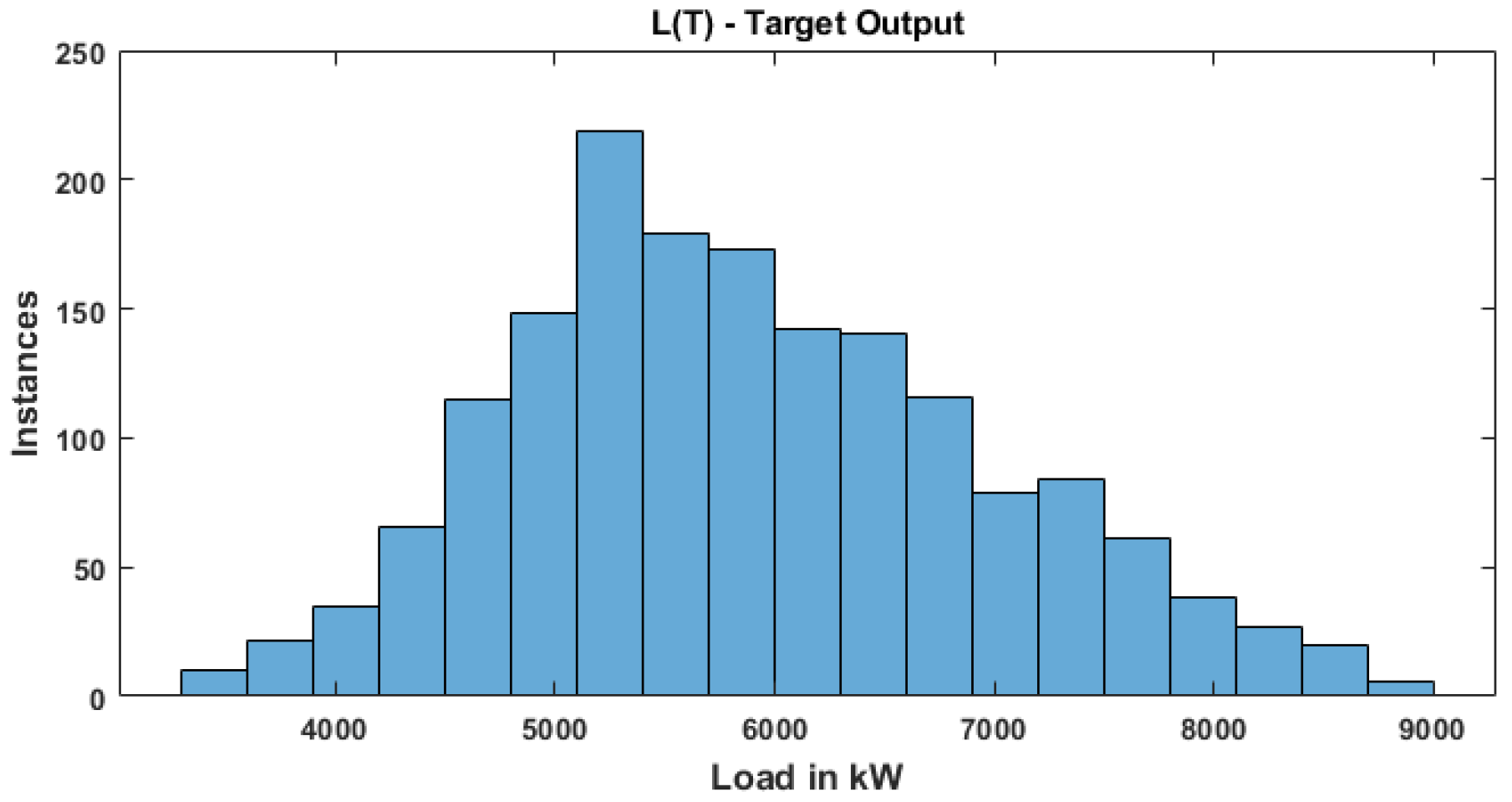
| Statistical Parameters | Output |
|---|---|
| Count | 1680.00 |
| Mean | 5904.52 |
| Std. | 1077.75 |
| Min | 3377.92 |
| 25% | 5138.90 |
| 50% | 5795.62 |
| 75% | 6618.66 |
| Max | 8841.67 |
| Number of training samples | 1512 |
| Number of testing samples | 168 |
| Nodes | Training | Testing | Trainable | |
|---|---|---|---|---|
| MSE | RMSE | MAE | Param | |
| 21 | 0.0104 | 0.124 | 0.093 | 673 |
| 18 | 0.0103 | 0.120 | 0.088 | 523 |
| 15 | 0.0102 | 0.115 | 0.081 | 391 |
| 13 | 0.0101 | 0.115 | 0.08 | 313 |
| 11 | 0.0102 | 0.117 | 0.083 | 243 |
| 10 | 0.0104 | 0.117 | 0.083 | 211 |
| No. of Hidden | Training | Testing | Trainable | ||
|---|---|---|---|---|---|
| Layers | Nodes | MSE | RMSE | MAE | Parameters |
| 1 | 13 | 0.01 | 0.115 | 0.08 | 313 |
| 2 | 13 | 0.01 | 0.124 | 0.094 | 664 |
| 3 | 13 | 0.01 | 0.131 | 0.1 | 1015 |
| Statistical Parameters | Training | Testing | |
|---|---|---|---|
| MSE | RMSE | MAE | |
| count | 10 | 10 | 10 |
| mean | 0.0103 | 0.1168 | 0.0831 |
| std | 0.000125 | 0.001751 | 0.003725 |
| min | 0.0101 | 0.115 | 0.079 |
| 25% | 0.0103 | 0.11525 | 0.08 |
| 50% | 0.0103 | 0.1165 | 0.082 |
| 75% | 0.010375 | 0.11775 | 0.08575 |
| max | 0.0105 | 0.12 | 0.09 |
| PC-1 | PC-2 | PC-3 | PC-4 | PC-5 | PC-6 |
|---|---|---|---|---|---|
| 1.15773 | −0.03658 | −0.15948 | 0.080498 | −0.03406 | −0.09375 |
| 1.206716 | 0.022011 | −0.06865 | 0.10224 | 0.020807 | −0.02302 |
| 1.317927 | 0.087764 | −0.15442 | 0.286619 | 0.173571 | 0.137578 |
| 1.474023 | 0.247519 | −0.14054 | 0.327771 | 0.017663 | 0.282082 |
| 1.585102 | 0.250539 | −0.10991 | 0.301018 | 0.04917 | 0.098137 |
| 1.528944 | 0.003412 | −0.09801 | 0.148669 | −0.02632 | 0.071544 |
| 1.675344 | −0.22242 | −0.34602 | 0.148969 | −0.08434 | 0.103249 |
| 1.571563 | −0.28011 | −0.51846 | 0.037141 | −0.23163 | 0.15251 |
| 1.335613 | −0.03608 | −0.48765 | 0.030066 | −0.05095 | 0.214678 |
| 1.035098 | 0.156347 | −0.3284 | 0.417524 | −0.17399 | 0.139219 |
| Hidden Nodes | Training | Testing | Trainable Parameters | |
|---|---|---|---|---|
| MSE | RMSE | MAE | ||
| 9 | 0.0111 | 0.122 | 0.089 | 154 |
| 10 | 0.0114 | 0.119 | 0.086 | 181 |
| 11 | 0.0110 | 0.117 | 0.084 | 210 |
| 12 | 0.0111 | 0.121 | 0.088 | 241 |
| 13 | 0.0110 | 0.121 | 0.089 | 274 |
| No. of Hidden | Training | Testing | Trainable Parameters | ||
|---|---|---|---|---|---|
| Layers | Nodes | MSE | RMSE | MAE | |
| 1 | 11 | 0.0110 | 0.117 | 0.084 | 210 |
| 2 | 11 | 0.0112 | 0.119 | 0.086 | 463 |
| 3 | 11 | 0.0113 | 0.12 | 0.088 | 716 |
| 4 | 11 | 0.0113 | 0.2 | 0.087 | 969 |
| Statistical Parameters | Training | Testing | |
|---|---|---|---|
| MSE | RMSE | MAE | |
| Count | 10 | 10 | 10 |
| mean | 0.0112 | 0.1194 | 0.0861 |
| std | 0.0001 | 0.0014 | 0.0018 |
| min | 0.0110 | 0.1170 | 0.0840 |
| 25% | 0.0112 | 0.1190 | 0.0850 |
| 50% | 0.0112 | 0.1190 | 0.0860 |
| 75% | 0.0113 | 0.1208 | 0.0868 |
| max | 0.0115 | 0.1210 | 0.0890 |
| Model | Trainable Parameters | Testing | |
|---|---|---|---|
| RMSE | MAE | ||
| RHM-1 | 313 | 0.115 | 0.080 |
| RHM-2 | 210 | 0.117 | 0.084 |
| % of absolute change | 32.91 | 1.7 | 5 |
| Hidden Nodes | Training | Testing | Trainable Parameters | |
|---|---|---|---|---|
| MSE | RMSE | MAE | ||
| 18 | 0.0155 | 0.1510 | 0.1140 | 469 |
| 15 | 0.0155 | 0.1500 | 0.1100 | 346 |
| 13 | 0.0155 | 0.1420 | 0.1030 | 274 |
| 12 | 0.0155 | 0.1460 | 0.1090 | 241 |
| 11 | 0.0155 | 0.1480 | 0.1100 | 210 |
| No. of Hidden | Training | Testing | Trainable Parameters | ||
|---|---|---|---|---|---|
| Layers | Nodes | MSE | RMSE | MAE | |
| 1 | 13 | 0.0155 | 0.142 | 0.103 | 274 |
| 2 | 13 | 0.0154 | 0.148 | 0.108 | 625 |
| 3 | 13 | 0.0156 | 0.148 | 0.109 | 976 |
| Statistical Parameter | Training | Testing | |
|---|---|---|---|
| MSE | RMSE | MAE | |
| Count | 10 | 10 | 10 |
| mean | 0.0155 | 0.1475 | 0.1089 |
| std | 0.0001 | 0.0040 | 0.0041 |
| min | 0.0154 | 0.1420 | 0.1030 |
| 25% | 0.0154 | 0.1440 | 0.1065 |
| 50% | 0.0155 | 0.1475 | 0.1090 |
| 75% | 0.0156 | 0.1498 | 0.1100 |
| max | 0.0157 | 0.1540 | 0.1160 |
| Hidden Nodes | Training | Testing | Trainable Param | |
|---|---|---|---|---|
| MSE | RMSE | MAE | ||
| 5 | 0.0165 | 0.145 | 0.107 | 56 |
| 6 | 0.0164 | 0.144 | 0.107 | 73 |
| 7 | 0.0165 | 0.143 | 0.106 | 92 |
| 9 | 0.0167 | 0.145 | 0.107 | 136 |
| 11 | 0.0164 | 0.146 | 0.109 | 188 |
| No. of Hidden | Training | Testing | Trainable Parameters | ||
|---|---|---|---|---|---|
| Layers | Nodes | MSE | RMSE | MAE | |
| 1 | 7 | 0.0165 | 0.143 | 0.106 | 92 |
| 2 | 7 | 0.0165 | 0.144 | 0.108 | 197 |
| 3 | 7 | 0.0166 | 0.150 | 0.114 | 302 |
| Statistical Parameters | Training | Testing | |
|---|---|---|---|
| MSE | RMSE | MAE | |
| count | 10 | 10 | 10 |
| mean | 0.0165 | 0.1465 | 0.1092 |
| std | 0.0002 | 0.0021 | 0.0029 |
| min | 0.0163 | 0.1430 | 0.1050 |
| 25% | 0.0164 | 0.1448 | 0.1065 |
| 50% | 0.0165 | 0.1470 | 0.1095 |
| 75% | 0.0166 | 0.1480 | 0.1115 |
| max | 0.0168 | 0.1490 | 0.1130 |
| Model | Trainable Parameters | Testing | |
|---|---|---|---|
| RMSE | MAE | ||
| RDM-1 | 274 | 0.142 | 0.103 |
| RDM-2 | 92 5 | 0.143 | 0.105 |
| % of absolute change | 66.42 | 0.7 | 1.9 |
| Model | MSE | RMSE | ||
|---|---|---|---|---|
| Training | Testing | Training | Testing | |
| ANN Model [29] | 0.29 | 1.59 | 0.54 | 1.26 |
| ANN Model [30] | 0.23 | 0.44 | 0.48 | 0.66 |
| ANN Model [22] | 0.2 | 0.32 | 0.45 | 0.57 |
| SLR Model [19] | 0.0973 | 0.0163 | 0.312 | 0.128 |
| PR Model [19] | 0.0171 | 0.0158 | 0.131 | 0.126 |
| MLR Model [19] | 0.0723 | 0.0119 | 0.269 | 0.109 |
| LSTM-HAM-Model1 [20] | 0.0109 | 0.013 | 0.104 | 0.114 |
| LSTM-HAM-Model2 [20] | 0.0125 | 0.0146 | 0.112 | 0.121 |
| LSTM-DAM-Model1 [20] | 0.0156 | 0.02 | 0.125 | 0.141 |
| LSTM-DAM-Model2 [20] | 0.0166 | 0.02 | 0.129 | 0.1414 |
| RHM-1 | 0.0101 | 0.0132 | 0.1 | 0.115 |
| RHM-2 | 0.011 | 0.0138 | 0.105 | 0.117 |
| RDM-1 | 0.0154 | 0.02 | 0.124 | 0.141 |
| RDM-2 | 0.0163 | 0.0205 | 0.128 | 0.143 |
| Parameter | [29] | [30] | [22] | RHM-1 | RHM-2 | RDM-1 | RDM-2 |
|---|---|---|---|---|---|---|---|
| Mean | 0.2975 | 0.2500 | 0.2250 | 0.0135 | 0.0143 | 0.0215 | 0.0215 |
| SD | 0.0200 | 0.0100 | 0.0100 | 0.0002 | 0.0003 | 0.0010 | 0.0006 |
| Min | 0.2800 | 0.2400 | 0.2000 | 0.0132 | 0.0138 | 0.0200 | 0.0205 |
| 25% | 0.2800 | 0.2475 | 0.2175 | 0.0133 | 0.0141 | 0.0208 | 0.0209 |
| 50% | 0.2950 | 0.2500 | 0.2200 | 0.0135 | 0.0143 | 0.0217 | 0.0216 |
| 75% | 0.3050 | 0.2525 | 0.2350 | 0.0136 | 0.0145 | 0.0221 | 0.0218 |
| Max | 0.3300 | 0.2600 | 0.2500 | 0.0139 | 0.0147 | 0.0232 | 0.0223 |
| Batch Size | RHM-1 | RHM-2 | RDM-1 | RDM-2 | No. of Back Propagations |
|---|---|---|---|---|---|
| 1 | 624 | 1167 | 820 | 1182 | 151,200 |
| 8 | 131 | 148 | 106 | 153 | 18,900 |
| 16 | 74 | 82 | 50 | 85 | 9500 |
| 32 | 24 | 24 | 33 | 47 | 4800 |
Publisher’s Note: MDPI stays neutral with regard to jurisdictional claims in published maps and institutional affiliations. |
© 2022 by the authors. Licensee MDPI, Basel, Switzerland. This article is an open access article distributed under the terms and conditions of the Creative Commons Attribution (CC BY) license (https://creativecommons.org/licenses/by/4.0/).
Share and Cite
Veeramsetty, V.; Chandra, D.R.; Grimaccia, F.; Mussetta, M. Short Term Electric Power Load Forecasting Using Principal Component Analysis and Recurrent Neural Networks. Forecasting 2022, 4, 149-164. https://0-doi-org.brum.beds.ac.uk/10.3390/forecast4010008
Veeramsetty V, Chandra DR, Grimaccia F, Mussetta M. Short Term Electric Power Load Forecasting Using Principal Component Analysis and Recurrent Neural Networks. Forecasting. 2022; 4(1):149-164. https://0-doi-org.brum.beds.ac.uk/10.3390/forecast4010008
Chicago/Turabian StyleVeeramsetty, Venkataramana, Dongari Rakesh Chandra, Francesco Grimaccia, and Marco Mussetta. 2022. "Short Term Electric Power Load Forecasting Using Principal Component Analysis and Recurrent Neural Networks" Forecasting 4, no. 1: 149-164. https://0-doi-org.brum.beds.ac.uk/10.3390/forecast4010008