Climate Change, Security, Sensors

1
IDASC—Istituto di Acustica e Sensoristica O. M. Corbino (CNR), 00133 Rome, Italy
2
IEVPC— International Earthquake and Volcano Prediction Center, Orlando, FL 32860, USA
3
IASCC—Institute for Advanced Studies in Climate Change, Aurora, CO 80014, USA
4
ISSO—International Seismic Safety Organization, Headquarters, 64031 Arsita (TE), Italy
Acoustics 2020, 2(3), 474-504; https://0-doi-org.brum.beds.ac.uk/10.3390/acoustics2030026
Submission received: 16 April 2020
/
Revised: 6 June 2020
/
Accepted: 29 June 2020
/
Published: 3 July 2020
(This article belongs to the Special Issue Wind Turbine Noise)
Abstract
:A concise threefold illustration is given: (i) of climate change on the gigayear (Ga) time scale through the nanosecond (nsec) time scale, (ii) of the role of the performance of solid materials, concerning both manmade and natural structures with reference to security, and (iii) of the exploitation of the electrostatic energy of the atmospheric electrical circuit—which is an enormous reservoir of natural “clean” energy. Several unfortunate misunderstandings are highlighted that bias the present generally agreed beliefs. The typical natural pace of the Earth’s “electrocardiogram”, ~27.4 Ma, is such that, at present, for the first time humankind must challenge an Earth’s “heartbeat”. A correct use of sensors is needed to get an efficient monitoring of the ongoing climate change. Both anthropic and natural drivers are to be considered. A brief reminder is given about sensors that ought to monitor solid materials—with application (i) to every kind of machinery, building, viaduct or bridge, vehicle, aircraft, rocket, etc. and (ii) for a correct (and unprecedented) monitoring of the electric field at ground, which is the prerequisite for the exploitation of the electrostatic energy of the atmosphere. In every case, a systemic approach is always needed. Every specialized investigation often misses the true physics of phenomena. The resulting great complication can be tackled by means of suitable approximate and “simple” models, which always have to be correctly tested. The impact on the biosphere is manifested as a steady regeneration of microorganisms at the deep ocean floors, supplied by endogenous CH4. Microorganisms are thus the beginning of an ever rejuvenating food chain. The natural climate change implies a permanent evolution of living forms. On the longer time-scale, a permanent cycle occurs of species extinction and/or generation. In addition, owing to such a process, some living forms are likely to also exist underground on other planetary objects. That is, life ought to be a ubiquitous intrinsic endogenic feature of matter in the universe, while life’s survival, evolution and/or extinction, ought to depend on the available hosting environment.
1. Introduction
The target of the present paper is to highlight—mainly to an audience of engineers—the need for unprecedented sensors aimed to monitor the environment and to improve security and welfare. A warning deals with the bias by “generally agreed” and “common” beliefs, and by an incorrect reference to non-tested “models” that rely on arbitrary simplifying assumptions.
The challenge is represented by an unprecedented ongoing rapid climate change. The concern is not about whether phenomena are unprecedented or not. There is just a need to face present events.
A concise illustration is given in three steps of a wide multidisciplinary item.
The first step deals with a list of basic observational facts concerning climate change. The main concern is about getting rid of the bias by a large amount of false “generally agreed” beliefs and misunderstanding.
The second step refers to the sensors that can provide an unprecedented, timely, and incisive monitoring of the performance of solid structures, with application to the security either of artifacts and/or of natural systems.
The third step deals with sensors for an unprecedented monitoring of the atmospheric electrical circuit. The ultimate target is the exploitation of the immense reservoir of the natural electromagnetic (e.m.) energy, exploitable through the electrostatic energy supplied by the solar wind. By a decade of correct observations, it will be possible to get the needed information aimed to exploit a free—huge and “clean”—renewable energy source, possibly with relevant impact on the global economy.
The term “environment” is here used to denote every given condition inside a given domain of space and/or time. In contrast, the term “climate” is here used to denote the domain of environment where the biosphere can survive and thrive. In this respect, note that the often used definition is here contended of “climate” identified with statistics of environmental parameters. Indeed, statistics cannot be identified with the rationale of the understanding of phenomena.
A basic warning is needed. I must apologize for the impossibility to give a full critical discussion. Only a very scant list is here given of references. In fact, it is impossible to synthesize the critical discussion in a few pages. An exhaustive treatment is given in an 8-volume set (about 13,000 pages), that at present is completed, to be published as soon as possible free on the web. Permission for use of figures and tables is presently being progressively granted. A preliminary presentation is given in Gregori (2014) [1]. In any case, I stress that we must always rely on observations. Leonardo da Vinci repeatedly - and in different ways - claimed that one should first “read the book written by Nature, and only later on the books written by men”. That is, every statement given here relies on observations—and a specific warning is made whenever some role is played by modeling.
Indeed, the often celebrated and fashionable “models” are a clever way to assess how far a given interpretation matches with observations. But, “models” are only clever mathematical exercises carried out by very skillful applied mathematicians. The basic understanding of processes and mechanisms cannot be given by a numerical model, that is rather only a way to test the limits of our understanding, i.e., of our ignorance. One should never confuse the role of different specialists: geophysicists, geologists, engineers, applied mathematicians. For instance, it is still widely claimed that the Earth’s inner core (IC) is “solid” because it is crossed by seismic S waves. This is a naïve belief by people who have no real feeling about some well-assessed knowledge of basic solid state physics. Such a misconception is generally supported by Earth scientists who rely on college physics, and on concepts that, since over one century ago, have been obsolete. As another example, meteorologists are highly professional and reliable applied mathematicians, who very carefully check the skill of their forecast, but refrain from extrapolating their prediction behind a well assessed time range. In fact, the basic present limitation of meteorology is likely to be related, perhaps, to the crucial role of e.m. phenomena, that ought to be better taken into account, in addition to the thermodynamic viewpoint that is presently considered. In any case, the reader must be warned and get rid of an ensemble of false and unproven, widespread paradigms.
Let me anticipate a few basic items to be better explained in the following.
The Earth is not a hot ball that is cooling in space on the Ga (gigayear) time scale. Rather, the Earth operates like a battery, with a varying recharging and discharging. Hence, the time scale of different phenomena is crucial (see below).
The space between the Sun and planets is not empty. Hence, solar–terrestrial relations occur through a twofold channel: (i) solar e.m. radiation, and (ii) corpuscular radiation, called solar wind, identified with the thermal expansion of the solar corona. Compared to e.m. radiation, solar wind variations are fundamental for the solar influence on planets, due to the solar wind control on the generation of endogenous heat.
Interstellar space inside the galaxy (Milky Way) is not empty. The encounters of the Solar System with clouds of matter are crucial for the control of solar activity and of the solar wind, hence of Earth’s climate.
No discontinuity exists between solar wind and Earth’s atmosphere. The natural system is just a continuum. Similarly, one must consider a unique, huge, system of electrical circuits encompassing altogether the Sun, solar wind, solar corona, the whole Earth’s system, through the entire Solar System, and inside the Earth’ body, down to the Earth’s center. A most “shocking” aspect is the steady presence of intense air–earth currents, i.e., electric currents crossing through the Earth’s surface. Note that for almost two centuries air–earth currents were basically neglected, according to a classical—and formerly quite reasonable, though unproven—working hypothesis by Gauss.
This whole electrical system is powered by the Sun, and by a tidal dynamo supplied mainly by the Moon. The energy is responsible for all phenomena that occur on the Earth. The exploitation of such an energy reservoir is a benchmark for the Earth’s global economy, for “climate”, and for the survival of humankind.
The fake concept of “primordial soup” where life was originated has to be rebutted. Life is endogenic and microorganisms are continuously regenerated everywhere. Whenever the environment is suitable for life’s development; the evolution occurs of higher life forms. On the Earth, microorganisms are observed to be steadily regenerated at the deep ocean floors, where no solar radiation can penetrate. The needed energy supply is by endogenous methane (CH4) exhalation. This is the start of the food chain. Increasingly complex living forms progressively occupy ever shallower ocean layers, where solar radiation is an additional energy-source that permits the “explosion” of unprecedented life forms. Thus, depending on climate change, different life forms steadily experience extinction while new forms are born. For instance, vaccines must be continuously regenerated.
Thus, every planetary object is to be expected to have life forms, although eventually only underneath its surface, whenever no sufficient amount of solar radiation is available, etc.
Therefore, climate and health are closely related to each other. The target is to exploit feasible and reliable sensors suited to monitor and to envisage suitable actions aimed to manage the “climate change”.
It should be stressed that humans are just one component of “climate”. The anthropic action can be either negative or positive. Every human action is a driver to be added to all other natural drivers. A correct understanding of phenomena, with no false paradigm, is the prerequisite to manage the hazards and risks of climate change and of natural catastrophes.
2. Energy and Mass—Detectability—The Empirical Constraint
Some basic, though uncommon but fundamental, premises are needed for the present discussion. The energy source is a primary concern, when attempting an interpretation of observations. Energy and mass are manifestations of a unique reservoir. Hence, while dealing with a general perspective, it is worthwhile to consider altogether mass plus energy, and to deal with “emp”—acronym for energy-mass-primordial.
Another concept is the “empirical constraint”, i.e., the concern about what we can really observe by means of our instruments. In this respect, chemical bonds are fundamental for biology and for our same existence. Hence, “climate” deals with a “cold” environment. Differently stated, electrons in atomic shells are fundamental. Electrons are responsible for the emission of photons that are the main source of our available observational information.
In contrast, inside a “hot” environment, even a state of total ionization must be paradoxically considered, where no photon can be released. In such an extreme state, “emp” cannot be directly detected. At most, we can infer its existence only through indirect evidence. This is the so-called “dark matter”, or plasma “dark mode” as opposed to “glow mode”, that perhaps is the most frequent state in the universe. But, it is likely that it is also the explanation of the inner core (IC) of the Earth. In this same respect, remind about the aforementioned naïve concept of “solid” IC: A likely hypothesis is that the IC is composed of atomic nuclei with no electron shell. Hence, these nuclei are strongly coupled to one another by their respective magnetic moments. Such a state of complete magnetic polarization can therefore be called “magpol”, in addition to other best known states of matter. The rigid magnetic coupling is such that also S waves can easily cross through the IC, even better than through a solid body. The IC ought thus to display some kind of “fibrous” structure, and the whole pattern ought to be responsible for the origin of the leading dipole magnetic field of the Earth.
A concise summary, from small through large object, is as follows dealing with energy sources. But, a long historical debate ought to be recalled (radioactivity, fossil heat, biomass, etc.), which is however only a curiosity. In addition, the existence of gravitation is here taken for granted, as its discussion is outside the perspective of the topics that are here considered.
2.1. The Tide-Driven (TD) Dynamo—The Earth Like a Battery
Consider an object that is composed of parts (either solid or fluid), and suppose that the components can move relative to one another. In addition, suppose that the entire system experiences a local gravitational gradient. Note that, unlike the intensity of gravitation, the gradient is relevant to causing relative displacement of different components (e.g., the gradient of the lunar-tide is well-known to be more effective than the solar-tide gradient).
In general, matter is partially ionized, the whole process thus results to be an effective dynamo (Gregori, 2002, 2009) [2,3], i.e., the tide-driven (TD) dynamo. But, in addition to the gravitational gradient, the TD dynamo is controlled by the e.m. induction by the solar wind that affects the stator of the dynamo.
The present energy balance referred to the Earth – in fact, the TD dynamo applies to all planetary objects (see below)—is given in Table 1 and in Figure 1. The enormous e.m. energy is to be stressed, which decays by Joule heat (see below), while only a tiny, almost negligible, fraction is observed like geomagnetic field. In this respect a remind is deserved about the present generally agreed explanation for the origin of the geomagnetic field, that is generally reported in the literature. That explanation relies on an MHD dynamo (the so-called Elsasser–Bullard dynamo), which is the application to a planetary object of the Larmor dynamo, which correctly applies inside a star. But, the identical mechanism is physically untenable inside a planet. The criticism can be simply explained upon considering a standard dynamo of a hydroelectric plant. The amount of water that is injected in the dynamo depends on the amount of power that is absorbed by the users. In fact, if water is supplied even when no user-absorption occurs, the dynamo ends up in a total blocking by the enormous magnetic forces that couple stator and coil. In the case of the Sun, this effect is called Biermann’s blocking (as Biermann first stressed this phenomenon inside sunspots). However, the endogenous thermonuclear energy, which is typical inside every star, causes a violent disruption of the blocking (see Section 2.3). The same process cannot occur inside a planet, as no thermonuclear process is in progress. All numerical MHD models computed for a Elsasser–Bullard dynamo in the Earth unavoidably always lead to numerical blocking, unless “suitable” arbitrary perturbations are mathematically speculated, etc. (Gregori, 2002, [2]). For brevity’s purpose, only two issues are here stressed.
The whole scenario of the Earth system is thus dominated by a tremendous amount of endogenous energy. The Earth is a battery that is steadily recharged by the TD dynamo, with a modulation originated by the e.m. induction by the time-varying solar wind flow. The timing is therefore crucial to the battery discharge. The most relevant energy release occurs through the ubiquitous geothermal heat, and its time-variation plays a primary role for climate change.
As far as the solar–terrestrial relations are concerned, reference has therefore to be made (Figure 2) to a twofold process, i.e., an “external way” by solar e.m. radiation that penetrates through the atmosphere, and an “internal way” by the solar wind that modulates the generation of endogenous energy, altogether with the time-delayed energy release by exhalation into the ocean/atmosphere’s entire system with an impact on “climate”.
The timing of the battery discharge is explained by the fact that every electric circuit expands in space as much as possible (in college physics this is the Hamilton variation principle). That is, electric currents are generated inside deep Earth by the TD dynamo. Every circuit attempts to expand as much as possible, depending on the local electrical conductivity σ. Finally, currents decay by Joule heat wherever they find an almost step-like drop of σ. Every drop can be approximately denoted as a σ discontinuity. Step-like drops can indeed be monitored by means of the geomagnetic field (Gregori, 2002, 2009) [2,3]. A confirmation of this interpretation is provided by independent estimates, of the depth of these well-known step-like transitions inside deep Earth. A coincidence is thus verified of estimates by seismology and by geomagnetism. In addition, the secular variation of the geomagnetic field permits to detect the large changes vs. time of the radius of the Earth’s IC. This is the mechanism for the time-variation of the energy storage in the Earth battery.
A surface of σ discontinuity is, however, not perfectly spherical. Thus, owing to Hamilton, every minor bump (Figure 3) of such a surface implies a larger concertation of electric current right at the very top of the bump, where Joule heat is generated. Thus, σ is locally increased and the σ discontinuity can expand. The process reminds us about an electric soldering iron that is pushed inside a block of ice (ESI mechanism). Thus, a spike is generated, and the Earth’s interior finally reminds us about a sea-urchin.
When a “spike” approaches the Earth’s surface, as soon as some fluids (water, oil, CH4, geogas, etc.) are available, fluids can transport heat by advection. However, when fluids are insufficient, the local temperature increases and the “spike” further propagates upward. When the spike reaches some shallow depth of a lower lithostatic pressure, where equation-of-state permits melting, a new fluid is formed, i.e., magma, which samples the basalt chemism of the layer where it is formed. Indeed, the isotopic chemism of ocean basalt is useful information suited to check the whole process. The magma is just another fluid that, through an eruption, transports heat by advection.
The “sea-urchin spikes” have a twofold role: (i) they are effective channels for the energy transfer from deep Earth through Earth’s surface, and (ii) they are efficient antennae for the e.m. coupling between solar wind and deep Earth, thus permitting the modulation of the TD dynamo. In fact, in this way, the Faraday screening is avoided by shallow Earth’s layers. In addition, the mutual interaction between sea-urchin spikes seems to also give an unexpected explanation for the planetary distribution of mid-ocean ridges (MORs).
2.2. An Approximate Model
Science is the conquest of understanding, and—like every conquest—science needs outposts conquered by selected attack-troops, followed by systematic reorganization of the conquered land. Approximate models are “simpler”, hence better suited to exploit “intuition” and to attack.
I stress that the results that are here presented derive from a rigorous critical reorganization of a “land” that was suffering by logical gaps, inconsistencies, paradoxes. But, a mention is deserved for a present outpost-trench concerned with the long-period e.m. induction by the solar wind. A reminder is given about two items.
Consider that solar e.m. radiation is usually treated in terms of e.m. waves of a given frequency, where every “ray” is composed of an endless number of complete waves. In contrast, solar wind is responsible for e.m. induction at some unbelievably long period. Hence, only transient perturbations occur that span a time lag much shorter than a wavelength. Therefore, the concept of “wave” is only mathematical and can be misleading. Transient perturbations are rather to be considered.
Thus, e.m. induction phenomena can be more expressively represented in terms of a transient change in total axial field strength of the Earth’s magnetic field. The transfer of energy approximately affects three primary vectors of Earth’s circuitry i.e., the vertical, orthogonal or radial, and axial fields, in different ways depending on the primary amount of vector-field change by the solar wind. Thus, e.g., the “internal way” is interpreted as a change of the total axial field strength, as a modulation of the radial component of the field. This is the “Stellar Transformer” approach. See Leybourne and Gregori (2020) [6] for details.
Another warning deals with the dichotomy continuum/quantum, i.e., between continuous functions and corpuscular solar wind. The best-known classical treatment relies on MHD (magneto-hydrodynamics), which is the classical gas theory, also including e.m. interaction. Max Planck solved the paradox of the black body spectrum by rejecting the continuum hypothesis. Similarly, paradoxes are also originated in solar–terrestrial relations. For instance, the best-known example deals with the concept of “reconnection”, i.e., magnetic field lines are supposed to “break” and to “reconnect” with a different topology. This is a denial of the Maxell’s law div B = 0. The correct physical reason is that the solar wind has particle/particle vacancies (“plasma cavities”). Hence, on the microscale, MHD is conceptually incompatible with the composition of the physical system. “Reconnection” is just a mathematical ad hoc trick.
MHD is a difficult discipline, with several distinctions, depending on the characteristics of the medium. Several excellent textbooks are available, e.g., Shercliff (1965) [7]. But, these items are not here pertinent, even though the scientific community seems to miss a correct perception of this basic drawback. For instance, reference ought to be made to the strictly local phenomena that originate either an instability, or a so-called electric double-layer, etc. These concepts are pertinent whenever the continuum approximation can be applied, and are useful mathematical tools aimed to represent the ongoing local phenomena according to the MHD viewpoint. In contrast, whenever discrete particle effects enter into play, the available number should be considered - on an instant basis - of the interacting particles. Variations occur on the time-scale of the time-lag spent by a light ray to cross through the distance between contiguous particles. Hence, the formalism of MHD is eventually paradoxical—and they eventually tried to “save” the formalism by introducing some additional paradox (such as the aforementioned “reconnection” hypothesis).
In any case, in principle, these eventually useful algorithms cannot be considered inside the rigorous critical reorganization that is here reported.
2.3. A Nuclear Reactor
A nuclear reactor ought to be considered inside suitably large planetary objects. Probably, at present, this occurs inside Jupiter, maybe also inside Venus. A nuclear reactor perhaps also existed inside the Earth during the first 2–2.5 GA of its existence, being the unique presently available possible explanation for the mysterious observed 3He/4He ratio in rocks.
2.4. Thermonuclear Reactions
When a celestial object is sufficiently large, thermonuclear reactions occur and a great amount of energy is generated by nuclear fusion and fission. This typically applies inside a star, which is characterized by a violent internal MHD that, owing to the large ionization, leads to Biermann’s blocking. But, owing to the huge endogenous energy production, the energy balance requires a breaking of the blocking. This results in a steady “explosion” of the star.
2.5. Two Basic Concepts—The “Principle Of Limited ‘emp’ Density”, and the “Cowling Dynamo”
A universal physical “principle” seems to play a key role through the whole universe. No formal proof is however at present available, although it seems to be confirmed by every observed case history.
The “principle” refers to the space density of “emp”, which can never exceed a physical threshold. But, at present it seems impossible to give a quantitative estimate for such a threshold. Differently stated, whenever, owing to some process, the “emp” density ought to violate such a principle, some new process must occur. For instance, owing to this principle, one can explain the limit of compressibility of matter, or why matter has to expand when heated, etc.
The second concept deals with a “universal theorem” that applies to the transformation of kinetic energy into e.m. energy. The theorem can be rigorously proven. The original proof, relying only on a lengthy application of college physics, is given in Gregori (2002) [2], where, however, it is not explicitly named and focused. In fact, at that time I was not yet aware of the relevance of this result. The mechanism derives from the generalization of the classical Cowling theorem and can be called the “Cowling dynamo”. It states that wherever an ionized medium experiences a relative motion, the kinetic energy is always transformed into e.m. energy, only according to either one of two configurations shown in Figure 4.
Both configurations are at equilibrium. But, case (a) with poloidal B and toroidal E is unstable, while case (b) with toroidal B and poloidal E is stable. However, in case (b) and in the hypothetical case of perfect cylindrical symmetry of the physical system, the total energy is null of the stable dynamo configuration (thus giving justice for the former paradoxical classical non-generalized Cowling theorem).
This theorem implies a magnetic self-confinement of every ionized medium. The application is ubiquitous at every scale-size through the universe. This is the explanation of a huge ensemble of phenomena, ranging, for example, from the filamentary patterns either of galaxies inside galactic clusters, or of stars inside a galaxy, through a previously non-understood self-alignment observed in the solar wind, through the linear pattern of a spark or of a lightning discharge, through the explanation of the mysterious ball lightning, through the mechanism that determines water condensation and precipitation in meteorology, etc. In this same respect, a related, although independently derived (Scott, 2015 [8]), evidence is concerned with the self-collimation of the so-called Birkeland currents, i.e., electric currents that flow along magnetic field lines. They display polygonal patterns observed either in the polygonal pattern of several cratering phenomena on the Earth and on other planetary objects (Burn, 2015 [9]), or in some “skeletal” pattern observed in cosmic dust clouds (Rantsev-Kartinov, 2020 [10]).
The Cowling dynamo applies to every scale-size both in space and time. It is rigorous as far as Maxwell’s laws can be applied, i.e., only in sub-atomic phenomena the theorem cannot applies, where quantum effects, Feynman graphs, etc. are to be considered.
2.6. A synthesis—Energy balance and Exploitation
Figure 5 shows the global energy flow-diagram. A unique huge electrical circuit crosses through the whole natural system from the Earth’s center through the Sun’s interior and up to the boundaries of the Solar System.
As far as the Earth is concerned, the primary energy supply derives from lunisolar tide, while the solar wind modulates the efficiency of the production rate of endogenous energy by the TD dynamo. In addition, the flow of the solar wind is modulated by the encounters of the Solar System with clouds of interstellar matter.
The currents that flow through the overall electrical circuit generate everywhere Joule heat that originates convection through fluids. Thus, owing to the ubiquitous Cowling dynamo, whenever the medium is ionized the thermal/kinetic energy is transformed into e.m. energy.
The enormous available amount of energy is responsible for the whole set of geodynamic, volcanic, geothermal, climatic and environmental phenomena of the Earth (as per Figure 1). We can—and we must—exploit energy, i.e., we should intercept the electrostatic energy associated with the ubiquitous air–earth currents at Earth’s surface.
3. Time Scales
As a premise, when we refer to a phenomenon, a basic distinction (“forcing/recovery”) depends on whether the effect is the result of the forcing by an external action, or rather it is the response while the system recovers after a previous stress.
In fact, every phenomenon requires a non-vanishing time lag, i.e., nothing is “instantaneous”. For instance, consider the “hammer effect” (see below; i.e., the system behaves differently during a hammer strike and during subsequent elastic/plastic recovery). But, the same concept applies to the response of a volcano etc.
Another distinction (“calorimetric effect”) means that the system, during some time lag, stores energy in a reservoir until a threshold is attained, when a new process is triggered. Then, the system releases the stored energy during another time lag, before charging anew, etc. The simplest example is a pressure cooker: the safety valve whistles when the pressure affords to lift the valve.
The observed phenomena are here listed referring to different time scales. The available observational data base is here recalled only whenever it is not yet commonly known.
3.1. The Time Scale of 109 Years (GA)
A key role is played by the encounters of the Solar System with interstellar clouds of matter (ICMs); see Figure 5.
The Sun is located at ~30,000 LYs (light years) from the center of the Milky Way (which has a radius, say, of ~100,000 LYs and a thickness of, say, 300–400 LYs). The Sun rotates around the center of the galaxy with a period of ~280 Ma (or ~250 Ma). See Figure 6. Based on an analysis of the magma production rate by the Hawaii volcanism, a ~14 Ma period is found that seems to be associated with an oscillation of the Solar System with respect to the galactic equatorial plane. Every crossing implies an encounter with denser ICMs, that are the forcing agent for the TD dynamo.
The Sun has a magnetic shield, analogous to the Earth’s magnetosphere. The shield is called the heliosphere. A dense ICM can even compress the heliosphere (hence the solar wind) inside the Earth’s orbit. The associated violent e.m. induction inside a planetary object—originated by a temporary disappearance and reappearance of the solar wind—determines a violent generation of endogenous Joule heat.
This is the explanation of the mysterious geomagnetic field reversals (FRs) recorded on the Earth. Note that the “magpol” IC moves inside the outer core (OC) where, however, friction occurs only through e.m. coupling. Hence, whenever the ambient B field has been substantially weakened or cancelled by the e.m. induction from the solar wind, the IC can move freely, almost with no “friction”. That is, the IC can flip North/South such as it occurs during a FR. Or the IC can also only partially overturn before returning to the original orientation, such as it is observed during a so-called “geomagnetic excursion”. The pace of these events is erratic, due to the negligible cross-section (~0.45 × 10⁻⁹) of the expanding solar corona, that is intercepted by the Earth’s magnetosphere.
The same phenomenon occurs on every planetary object where a TD dynamo is operative. In fact, as expected, in all planetary objects of the Solar System a close correlation is found between observed tectonism and endogenous magnetic field. In particular, the Pluto/Charon system is a natural laboratory suited to test the whole mechanism, because an enormous gravitational gradient is combined with a highly eccentric orbit, with consequent intense variation of the modulation by the solar wind. The extremely unusual tectonism of Pluto and of Charon thus envisages a unique seasonal dependence of the observed surface morphology (Gregori, 2016 [12]).
3.2. The Time Scale of 107 Years (10 Ma)—Earth’s Electrocardiogram—Superswells and LIPs
A calorimetric phenomenon is documented by the magma emplacement rate by the Hawaii hotspot. The Hawaii Islands are the youngest elements of a set of 108 seamounts (the Emperor Seamounts Chain). The drift of the lithosphere, which moves over the hotspot much like on a conveyor belt, determined the generation of the 108 seamounts in a regular times series. Thus, volumes and ages of the 108 seamounts are a record of the time change of the magma emplacement rate by the hotspot. The result is the Earth’s “electrocardiogram” with a typical period of ~27.4 ± 0.05 Ma (Figure 7).
The two plots show, respectively, from top to bottom, the volume Q of magma emplacement, and the speed v of the lithosphere relative to the hot spot source. The data base does not permit a 10,000 years resolution. One heartbeat occurred every ~27.4 ± 0.05 Ma, a trend that seems to have been a steady feature during the last ~250 Ma. On the occasion of every heartbeat, somewhere some huge magma flood was outpoured. The evidence is called “large igneous province” (LIP). Iceland is the LIP corresponding to the current heartbeat. When the hotspot yield increases, the number of elements of the chain is increased, rather than their respective volume, consistently with the calorimetric criterion.
Owing to the non-uniform release of energy by the sea-urchin pattern, the endogenous heat originates a different amount of thermal expansion of every continental-size region. Thus, a varying upheaval occurs at Earth’s surface. The result is the formation of huge macro-hills, called “superswells”. The lithosphere drifts on the slopes of superswells, sliding on a layer (ALB, asthenosphere/lithosphere boundary, or tout court asthenosphere) that is lubricated by a twofold effect (see below).
Different lithospheric slabs finally collide inside macro-valleys (called megasynclines) between superswells and determine continent formation and orogenetic processes. A better efficiency of the TD dynamo is thus responsible for greater geodynamic activity, volcanism, and exhalation into the ocean/atmosphere, thus affecting climate. The maximum observed drift speed of the Pacific lithosphere has been up to ~3 mm/day (Figure 7), consistently with the fastest case histories of continental drift.
Humankind’s history (say, ~20,000 years) refers to the present heartbeat. The present huge climate change, which is in progress, is unprecedented for the humans, and it can even intensify. It is impossible to state the timing of the maximum endogenous heat release. We only know that the maximum magma production rate occurs sometimes with a time-delay of ~50,000 years with respect to the heat generation by FRs, while no better estimate is possible.
3.3. The Time Scale of 104 Years (10 kA)—Terminations
The calorimetric behavior can be recognized also on much shorter time scales (Figure 8). According to several different records, often a climate warming occurred during some short time lag, followed by a slow climate cooling, even associated with an ice age. But, the same “sawtooth” trend can be recognized on much shorter time scales. That is, an energy reservoir recharges, while only a smaller amount of energy is released by the system. But, as soon as a release mechanism is “opened” that is suited to discharge the reservoir, a huge energy release occurs, and “climate” has a great energy content, dynamics, mean temperature, etc.
In particular, based on a few centuries of historical time series, volcanic activity can be recognized to display a cyclic trend, always according to the calorimetric rationale. But, the return time of the cycle is irregular, and, for every different volcano, it ranges between a few centuries to a few decades. The duration of every cycle is found to be correlated with solar activity (as inferred by tree rings). This result proves that solar activity is associated with a modulation of the TD dynamo etc., consistently with Figure 5.
3.4. The Time Scale of 103 Years—Mankind—Active and Passive Role—Environmental Anthropology
Humankind is just one component of the Earth system, with a twofold role: active and passive.
The active role is normally called pollution. The effect of pollution can be either negative when climate change is worsened, but also positive when catastrophes are prevented.
The passive role is associated with the recording of climate change. Records, however, are not homogeneous vs. time, depending on the improvement of monitoring techniques but also on the understanding of phenomena. A crucial role is therefore related to the cultural aspects of the understanding of the environment (hence, this is “environmental anthropology”). At every epoch, environmental anthropology is very important to optimize the anthropic impact on “climate”.
3.5. 10. The Time Scale of Years or Shorter—the Concern of the Man in the Street—Actions—Catastrophe Prevention and Management
The mean duration of human life is usually considered to be the reference time-scale. But, every natural phenomenon has an intrinsic timing. The concern of the man in the street is therefore concerned with annual phenomena, and he naively believes that every year ought to be similar to others.
In addition, it is believed that every effect or driver ought to be monitored at the highest precision and time resolution, as the ultimate concern of “science” ought to be the capability to forecast the future evolution of the system in order to prevent or to manage natural catastrophes. A correct understanding of phenomena—or rebutting false paradigms—is therefore essential for a correct management of hazards.
4. WMT, Geodynamics, Seismicity, Volcanism, Climate—Three Engines, Life and Biosphere
As far as “climate” is concerned, a few additional key issues are to be specified.
On the one hand, as mentioned above, the TD dynamo—which is powered by the tide and modulated by the solar wind—originates, through Joule heat at the top of sea-urchin spikes, a time-varying release of endogenous heat. A large spatial gradient causes a temporary formation of superswells and megasynclines. Slabs of lithosphere slide on the slopes of superswells, and eventually overthrust each other, generating continents and mountain chains.
At present, the highest elevation of superswells is approximately represented by the mid-ocean ridges (MORs), while a huge megasyncline is identified with the Pyrenees—Himalaya orogeny. Continents and mountains are periodically generated, and eroded by a comparatively rapid weathering. according to a cycle of, say, 100 ÷ 200 Ma, maybe of ~180 Ma (“Mortari cycle”). As a historical curiosity, Leonardo da Vinci had realized the rapidity of continent erosion, but he did not know about continent regeneration and steady orogenetic processes. Hence, he was quite concerned, and suffered profound nightmares (refer to his so-called “prophecies”).
As far as the lubrication is concerned, that occurs at the ALB (at a varying depth, typically say 80 ÷ 100 km depth ranging from a few ten to a few hundred kilometers), consider water penetration underground. An increase of water content is likely to be responsible for slower seismic wave propagation (this is the Moho). When water penetrates deeper through some fractured dry rocks, violent chemical reactions occur, with volumetric expansion by ~20%–40%, which originate new fractures, and additional water penetration. This process is known as serpentinization, and leads to the formation of the so-called serpentosphere.
Water, fracturing, heat, determine a greater electrical conductivity σ. Some electric currents that leak out from deeper layers’ decay by Joule heat at the top boundary of the serpentosphere. This is therefore a “lubricated” layer.
Hydrated rocks no more react with additional water. But, on the geological time scale, the endogenous heat determines a dehydration of rocks, that are thus ready for a new serpentinization.
Note the role of three engines (Figure 9). The TD dynamo is a physical engine, powered by the tide, while the serpentinization is the chemical engine. A third engine is biological, as solar irradiance amplifies the role of the food-chain within the conversion into biomass of the fluids and energy that are exhaled from soil. Biomass finally returns into ground in the form of organic sediments.
This whole geodynamic scheme is WMT (warm mud tectonics), as the Earth has an outer layer, the lithosphere, that slides on the inner layers, reminding us about some kind of mud heated underneath. Note that the often reported “plate tectonics” model is contradicted by several evidences. Hence, owing to several well assessed inconsistencies, plate tectonics is now harshly rebutted by a large number of specialists. This controversy is only a matter of history of science, not here pertinent.
The Earth can be illustrated as a battery, with varying charging and discharging times. The ~14 Ma timing of active modulation by the oscillation of the Sun with respect to the galactic equatorial plane, overlaps with the calorimetric phenomenon represented by the electrocardiogram. In fact, sea-urchin spikes penetrate through the Earth’s interior at a mean speed of ~10 cm/year, with maximum of ~20 cm/year for a sharper spike (Figure 3). After ~27 Ma, a suitable “way” is opened for the release of large amounts of endogenous energy. Thus, the battery can discharge. Finally, the energy release dramatically damps off, and a cool climate is observed (“sawtooth” trend). A heartbeat typically lasts, say, 4 ÷ 5 Ma, while the viscosity at the ALB also dramatically changes during such a cycle.
During several recent years an increase of seismic activity seemingly occurred, and (perhaps) also of volcanism. According to several independent evidences referred to a long time before the present, the whole northern polar cap seems to experience an ongoing general increase of endogenous heat release. That is, the whole Earth clearly seems to experience an increase of endogenous energy exhalation, with a violent impact on the dynamics of the ocean/atmosphere system. A more powerful ocean/atmosphere dynamic implies larger excursions (winds, atmospheric precipitation, hydrogeological anomalies, etc.).
But, another closely related effect is associated with wildfires that are mostly supplied by an increase of soil exhalation of CH4. Wildfires occur in areas covered by dry leaves, typically underbrush. Whenever some minor effect causes a very lesser and generally unobserved spark, CH4 permits the rapid generation of fire. The dramatic general fire that in the second half of 2019 hit whole of Australia ought therefore to be correlated with the increased seismicity of the whole large region through the Philippines and Indonesia. A movie of global wildfires (one frame every month for several decades) is available at NASA’s Earth Observatory. It displays some most interesting recurrent features that can be correlated with geodynamic indications. Arsons are a statistically insignificant set.
Observations unquestionably show the spontaneous generation of microorganism on deep ocean floors, where no solar radiation is available (Judd and Hovland, 2007) [15]. The energy supply is the ubiquitous soil exhalation of CH4. This is the beginning of the food web, as organisms of increasing complexity can grow up and occupy shallower layers of the ocean, until reaching a depth where solar radiation contributes a large amount of energy. The “primordial soup” concept is to be abandoned. Corals are developed downstream with respect to water currents that transport CH4. Life is endogenous and intrinsic in all matter. Also other planetary objects should have microorganisms underground, although, owing to lack of solar radiation, they eventually do not afford to get above surface.
New microorganisms are eventually generated depending on climate change. This explains the well-known and mysterious mutation of microbes that requires a continuous updating of the vaccines. In the larger scales of space and time, this implies that some living species eventually experience extinction while others are generated, as extensively documented by Earth’s history.
5. Monitoring Climate Change, False Beliefs, and the CO2 Concern
Climate change is the object of an increasing concern by mass media. But, several false information bias public opinion. Just a few items must be clarified.
The unicity of the system must be stressed. It is nonsensical to investigate separately atmosphere, ocean and solid Earth. Table 2 indicates some basic physical parameters (for brevity purpose, the same parameters referred to solid Earth are omitted, as here they are non-pertinent).
In this same respect, two basic warnings are to be stressed, concerning glacier melt, and sea-level change.
The equilibrium of an ice sheet either in Greenland or in Antarctica, or in a mountain glacier, is controlled by a sum of different drivers. The interpretation looks to be one of the most difficult challenges.
For sure, owing to the feeble thermal conductivity of ice, the increase of atmospheric temperature has a negligible impact. However, in general, a greater global increase in the release of endogenous energy implies a corresponding increase in water evaporation into the atmosphere. A greater amount of water in the atmosphere implies greater precipitation to occur somewhere. It is generally guessed that an increase in precipitation occurs over the so-called Eastern Antarctica where, in fact, the ice sheet is increasing. Ice sheet retreat is reported to occur in the so-called Western Antarctica, where a large local release of friction heat is expected by the huge geodynamic activity of the Antarctic Peninsula. Thus, the weight increases of the Eastern Antarctica ice sheet. Then, gravity pushes from upstream and speeds up the glacier flow towards the ocean.
Whenever an ice sheet flows downslope from a continental region (such as, for example, in Greenland or in Antarctica), as soon as the ice sheet reaches the ocean, it floats, thus looking like a huge “tongue” with an almost perfect half-circle outer-edge. Such an ice sheet is called an “outlet glacier” that, owing to ice cohesion, is constrained by an outer circular belt. Whenever the belt abruptly breaks, a large number of huge icebergs is released. Hence, the often reported statement is just ridiculous about iceberg generation being caused by an increase in atmospheric temperature.
As far as the sea-level change is concerned, the strict incapability must be stressed to estimate the total amount (hence also the time-change) of the water content stored either in the atmosphere, or in the oceans, or underground (down to the serpentosphere).
In addition, we are incapable of estimating the large-scale uplift, or subsidence, of large regions, according to the WMT rationale. For instance, a tilt is in progress by which the Iberian Peninsula uplifts, while the Aegean Sea subsides. Thus, sea-level is observed to decrease in Spain and to increase in Greece, etc.
Therefore, the time series of sea-level recorded at any given site can depend either on the time change of the total water content in atmosphere/ocean/subsoil, or also on the local tectonism of the recording station.
In summary, ice sheets and glaciers, and sea-level change, are unreliable gauges for climate change. In addition, it is well known that no single index or parameter can characterize the “world climate”—much like the body temperature, or any other index alone, cannot characterize the body’s health.
A great emphasis is generally given to the greenhouse effect, which is one—although not the main—driver of “climate” (much like the body-temperature is not controlled only by the clothes one wears). The greatest merit of the greenhouse effect is to damp off and smooth the largest climatic excursions. Every gas contributes to the greenhouse effect, the main role being played by H2O, while CO2 and CH4, which are also of anthropic origin, are reported as the second and third main greenhouse gases. The total amount, however, is important, because, at equal concentration per unit volume, CH4 has 23 times the warming potential of an equivalent amount of CO2 (Pappas, 2016 [16]). In addition, N2O, which is naturally formed by UV solar radiation, is 300 times more powerful than CO2, etc.
In any case, both CO2 and CH4 are a ubiquitous exhalation of endogenous origin. They are an essential component of the global carbon cycle. This argument is called the “principle of preservation of life” (Ronov, 1982 [17]) that claims that life ought to disappear with no exhalation of carbon gases. In fact, carbon is the primary fuel for the biosphere that captures carbon from the ocean/atmosphere, transforms it into organic material, which is later deposited in sediments, where it is eventually metamorphosed and exhaled by the endogenous heat, according to the aforementioned biological engine (Figure 9).
In general, however, the concern is about the ongoing steady increase of the CO2 atmospheric concentration. On the other hand, according to several evidences (e.g., Levenspiel, 2000 [18]), large variations occurred on the geological time scale of the atmospheric total density, and also of CO2 concentration. The physical mechanisms can be explained, although they cannot be here illustrated. The rationale is the balance between the stripping of atmosphere during a FR, and the time variation of endogenous energy exhalation.
A rough indication is that the atmospheric density was sometimes even ~12 times the present value. For instance, one of the best known paradoxes is the incapability of flying dinosaurs to lift up in the present atmosphere, depending on weight and on improper bone composition. Owing to Archimedes, their extinction likely occurred when atmospheric density was too low.
But, concerning the observed trend of the CO2 atmospheric concentration, two comments are needed.
The famous Mauna Loa time series is often claimed to be indicative of the role of anthropic CO2. It is forgotten, however, that the Hawaii Islands are located in a region with a maximum exhalation of endogenous heat. That is, the Mauna Loa time series shows that at present we live during the raising phase of a heartbeat—and the big wildfires in Australia in the fall of 2019 are one additional dramatic confirmation.
Similarly, it is complained that according to Antarctic ice cores, the present CO2 concentration had no equivalent during, for example, 400,000 years. Indeed, 400,000 years ought to be compared with the 27.4 Ma period of the electrocardiogram. That is, records on several ten Ma can be provided by volcanic islands, not by ice cores.
In addition, in some recent years, greenhouses were studied, where vegetation was grown inside an atmosphere with artificially increased CO2 concentration. Thus, brushes that with standard conditions grow a few ten cm tall, grew up to a few meters in size. Hence, CO2 availability greatly favors an “explosive” growth of vegetation, consistently with Ronov’s principle of preservation of life.
On 2 July 2014, NASA launched the satellite Orbiting Carbon Observatory-2, or OCO-2, which gave the first available map of CO2 concentration in the atmosphere. The seasonal maps (Figure 10) are a way to test the role of anthropic CO2 production compared to natural CO2 exhalation.
The Springtime map (Figure 10a) shows a huge maximum through the whole of northern Eurasia, mostly in the Arctic cap, consistently with the aforementioned great geothermal flow. During springtime the permafrost layer melts, and all gas that was confined underground during winter time can thus get out into the atmosphere.
The Summer map shows the paramount importance of vegetation as a sink for CO2. The role is fundamental of the green cover at Earth’s surface.
The Autumn map, in terms of astronomical symmetry, ought to be expected to be North/South symmetric and similar to the Springtime map, with reversed poles. In contrast, the observed map is totally different, clearly suggesting a paramount role played by permafrost.
The Winter map should be compared with the Springtime map, upon taking into account the frozen permafrost layer. In eastern North America, in Europe, and mainly in China/Japan, some contribution could be of anthropic origin. But, some concern deals with North Atlantic and North Pacific. In any case, the strong belt in equatorial Africa is certainly by natural exhalation.
In summary, the anthropic CO2 is a lesser driver in climate change, or maybe it is even negligible. Indeed, humankind must challenge an unprecedented and huge climate change due to natural drivers, and it is nonsensical to believe that a reduction of anthropic CO2 production can reduce hazards.
A distinction must be made between a “political” and true scientific—and not just fashionable—motivation. In this respect it is worthwhile to report the witness of Robert E. Stevenson (1921–2001), one of the most authoritative oceanographers of the XX century. During 1987–1995 he was Secretary General of IAPSO (International Association for the Physical Sciences of the Oceans).
Stevenson (2000 [20]) recalls the 1991 IUGG (International Union for Geodesy and Geophysics) General Assembly in Vienna, when they discussed a program to be proposed to ICSU (International Council for Science, formerly International Council of Scientific Unions). No program was submitted, and Stevenson (2000 [20]) paraphrases as follows their joint (and certainly very authoritative) statement: “to single out one variable, namely radiation through the atmosphere and the associated ‘greenhouse effect’, as being the primary driving force of atmospheric and oceanic climate, is a simplistic and absurd way to view the complex interaction of forces between the land, ocean, atmosphere, and outer space … climate modeling has been concentrated on the atmosphere with only a primitive representation of the ocean … actually, some of the early models depict the oceans as nearly stagnant. The logical approach would have been to model the oceans first (there were some reasonable ocean models at the time), then adding the atmospheric factors. Well, no one in ICSU nor the UNEP/WMO (United Nation Environment Program/World Meteorological Organization) was ecstatic about our suggestion. Rather, they simply proceeded to evolve climate models from early weather models. That has imposed an entirely atmospheric perspective on processes which are actually heavily dominated by the ocean.”
In any case, e.g., when dealing with cancer, one relies on oncologists, while one refrains from appealing to applied mathematicians, or to economists. Much like cancer cannot be tackled by means of mathematical models, in no way is climate change simpler than human pathology. No real progress seems was made after 30 years of additional self-claiming “scientific” discussion and “global climate models”. It is unbelievable that at present some very fashionable “common agreement” relies on numerical climate models, or on discussions by economists.
6. Perspectives
At present, we live during the maximum phase of an Earth’s heartbeat. The associated LIP has been the birth of Iceland that 2 Ma ago did not exist. A heartbeat typically implies an anomalous large release of endogenous heat during ~4–5 Ma. Hence, humankind (during, say, ~20,000 years history) is now facing a climate emergency that is totally unprecedented.
The timing of the maximum endogenous energy release cannot be predicted with a precision higher than, say, ~50,000 years. In addition, a time delay is to be expected of the order of ~50,000 years between the maximum energy supply by the TD dynamo and the output observed by magma outpouring. Hence, it is impossible to make any timely prediction.
Two heartbeats ago ~55 Ma ago, during ~4–5 Ma the Arctic Ocean was covered by subtropical vegetation: it was the origin of coal, CH4 and oil that is presently mined. But, it is claimed that, unlike at present, ~55 Ma ago the continent distribution was such that ocean circulation amplified the climatic effect. Hence, at present there seems to be, perhaps, no reason to be concerned about any similar anomaly.
On the other hand, several independent and indirect evidences envisage that, at present—and since a long time ago, maybe even in the geological time-scale—the whole northern polar cap is experiencing a steady increase vs. time of endogenous heat release (see, e.g., Figure 10a). In particular, this should explain the observed impressive melting of the Arctic ice sheet.
Glacier melt and sea level change are unreliable indicators, while, as far as the seismic and/or volcanic historical records are concerned, a different kind of difficulty has to be considered.
Seismic series are biased by the steady improvement of recording technology, and by a denser monitoring network. Hence, every trend vs. time is biased. Volcanic series are biased by the past belief that activity is just the “normal” state of a volcano. Thus, eruptions were not recorded. In addition, the typical timing of volcanic activity occurs on a multi-secular time-scale, which is much longer than the available historical record.
In any case, in recent years, several indications are generally reported that envisage a likely and significant large increase of seismic—and maybe also of volcanic—activity. This inference is consistent with the aforementioned WMT mechanism, by which an increase in the release of endogenous heat causes an uplift in superswells, an increase in geodynamics, in friction heat, and in global seismicity.
Moreover, the 2019 tremendous anomaly of Australian wildfires seems to be indicative of a large increase of CH4 exhalation. Hence, every accidental local overheating can trigger a fire that is strongly supplied by the available CH4. Such a very anomalous and unprecedented occurrence seems to be consistent with such a disquieting general rationale.
In summary, we should be prepared from the perspective of an ever increasing and dramatic climate change, and we must therefore consider suitable actions to prevent unwanted consequences.
In any case, claiming that everything occurs due to the anthropic CO2 is naïve and certainly false.
Rather, we must be concerned with anthropic pollution. But, the impact of different pollutants has to be assessed. For instance, the Covid-19 pandemic seems to be influenced by NO2 atmospheric concentration (Frontera et al., 2020 [21]). We must also consider that a proper pollution can have a positive impact on climate change. In this respect, for the time being, two concrete actions can be envisaged and are here briefly discussed.
One action deals with the management of loss of performance of solid materials. This applies to the twofold hazard, associated with the ageing of natural settings (seismic, volcanic, landslide hazard) and of manmade structures (machinery, concrete or metal viaducts, buildings, vehicles, etc.). This is discussed in Section 6.
Another action deals with the exploitation, discussed in Section 8, of the electrostatic energy of the atmospheric circuit (Figure 5). In fact, a huge and ubiquitous reservoir is freely available of a clean natural energy, that is potentially capable of substantially changing the management of climate, even in countries that at present are severely biased by starvation and poverty.
7. AE Monitoring—Seismic, Volcanic, and/or Hydrogeological Hazard, and Security of Manmade Structures
“Climate” is a domain of “environment”, where life forms can survive. Hence, the ambient temperature allows for the existence of crystalline bonds, i.e., of solid structures. Therefore, a large number of sources of hazards, and of security, is related to monitoring the loss of performance of solid materials due to ageing. The key information can be monitored by means of ultrasounds—conventionally denoted as “acoustic emission” (AE)—that are released by a solid lattice whenever a crystalline bond yields. Note that smaller flaws emit comparatively higher frequency AE.
The leading principle can be expressively and rigorously expressed by a simple example. Imagine staying inside a huge 3D construction-scaffolding, and watching in real time every breaking of a beam. Similarly, imagine an observer, who is the size of an electron, being located inside a crystalline lattice. Thus, the observer can monitor the rupture of every crystalline bond. Rupture events permanently happen, due to the natural ageing of matter, depending, for instance, on thermal excursion and/or on simple interaction with a photon. For instance, it is well known that the surface of every material changes due to light exposure, etc. In fact, everything in the universe experiences ageing. This is the same as claiming that time always elapses along the arrow of time, or that the entropy of the universe is increasing, etc.
I do not repeat the details of AE monitoring and analysis. For that, I refer you to several papers. For methods refer to Gregori et al. (2002 [22]), Paparo and Gregori (2003 [23]), and Gregori and Paparo (2004 [24]); for application to samples in the laboratory or to viaducts refer to Braccini et al. (2002 [25]), Guarniere (2003 [26]), Biancolini et al. (2006 [27]), Gregori et al. (2013 [28]); for application to volcanoes refer to Paparo et al. (2004 [29,30]), Gregori and Paparo (2006 [31]), Ruzzante et al. (2005 [32,33], 2008 [34]); and for applications to seismicity refer to Lagios et al. (2004 [35]), Paparo et al. (2006 [36]), Poscolieri et al. (2006 [37], 2006 [38]), and Gregori et al. (2009 [39], 2010 [40], 2016 [41], 2017 [42,43,44]). Rather, I stress a few basic logical issues.
I—An internal natural clock permits the assessment of the correct chain of cause-and-effect. In fact, to my knowledge, AE are the unique presently known way suited to assess what phenomenon occurs first and what second, rather than vice versa. For instance, I remind you about the so-called “VAN method” (after the names of P. Varotsos, K. Alexopoulos, and K. Nomicos) who, in the middle 1990s, claimed that geoeletric precursors can forecast earthquakes. A great EU research investment in the Balkan peninsula finally failed to give any evidence, as it was realized that it is impossible to assess whether an effect is either a precursor or an aftershock of a previous earthquake.
In fact, the coalescence of smaller flaws into progressively larger cracks originates AEs of a progressively decreasing frequency. The reason is that every crack is associated with a typical “flaw domain” of unknown size that, however, is of steadily increasing dimension. Hence, the direction of the arrow of time can be recognized by a simultaneous monitoring at least two AE of different frequency, because an identical anomaly is observed first in the HF AE and subsequently in the LF AE. We typically used a HF AE at, say, 180–200 kHz, and a LF AE at, say, 25 kHz.
II—The sequence of recorded AE impulses, associated with a breaking of crystalline bonds, can be analyzed by means of the fractal dimension Dt of the time-series of events. Note that, owing to definition, it is always 0 < Dt ≤ 1. The physical principle relies on the fact that a crystalline bond is more likely to yield wherever the solid lattice is already weakened by previously broken bonds.
When Dt ≈ 1 it is concluded that the bond rupture occurs randomly, due either (i) to a non-aged and well-performing structure, or (ii) due to a steadily increasing external drivers (e.g., an increasing pressure by hot endogenous fluids in a volcano, as observed on Stromboli, or on Peteroa in the Andes leads to Dt ≈ 1).
Upon relying on a different viewpoint, note that the ageing of a solid structure is caused by the fatigue due to an applied stress. Thus, for example, a steel bar subjected to repeated bending is found to display progressive decreases of Dt, being clearly indicative of performance loss. Whenever Dt ≈ 0.45 the steel bar is observed either to break or to be very close to final rupture.
III—“Hammer effect” denotes the different kinds of response by a solid structure depending on whether it is subjected to an applied stress, such as during a hammer strike—hence, called a “hammer regime”—or rather it is recovering after having suffered by the stress. It is shown that, on an instant basis, it is possible to assess whether the instant AE release occurs during a “hammer regime” or a “recovery regime”. According to clear observational evidence, it was always found that AE release occurs only, and strictly only, during a “recovery regime”. See, for example, Gregori et al. (2007) [45].
IV—The “domino effect” is another relevant empirical finding, by which is was found that all observed case histories are suggestive of—and consistent with—the fact that (Gregori, 2013 [46]) a natural propagation occurs inside every crystalline structure, independent of the kind of material being considered. The interpretation envisages that the coalescence of a flaw generates a stress that propagates to the nearby lattice, and thus it triggers a new rupture of some bonds, with the release of new AEs. The phenomenon is observed to propagate at a typical speed of ~10 cm/sec, and it seems to apply from the continental size through a few ten centimeters of a steel bar. Note that, in principle, it is reasonable to extrapolate the “domino effect” even to smaller sizes, depending only on the capability to detect AE impulses of sufficiently short duration. In this respect, also remind about stress propagation inside the serpentosphere, thus involving a stress teleconnection on the planetary scale. The “channels” of more efficient stress propagation are identified with the features that—according to the untenable and well-known model of plate tectonics—are named “plate boundaries”.
V—Owing to the reliability and precision of AE records, and to the high instant-resolution, periodic phenomena can be investigated with great efficiency. At present, however, only occasional tests were successfully carried out, as no specific need requested to exploit such an investigation.
VI—The cross-comparison between applications to different natural systems, either in the lab or in the field, resulted in being very helpful to implement a more precise interpretation in every single case history.
As far as applications are concerned, let me distinguish between manmade constructions and natural structures.
As far as a manmade system is concerned, the identical physical principle applies to every solid material (alloys, concrete, cement, glass, wood, rubber, etc.). In particular, let me remind you about an unexpected finding that was inferred by stressing in the lab some maraging-steel blades, specifically casted for the VIRGO experiment. These blades are part of the so-called super-attenuator aimed to smooth unwanted oscillations of the optical components of the interferometric system. Different blades were separately monitored in the laboratory (Braccini et al., 2002 [25]) by recording AEs released while a blade was bent and brought to standard performance (50 kg load). When a blade was bent for the first time after casting, it was found that Dt ≈ 1. Then, it was found that Dt decreases by ~0.1 in every successive bending, until the blade attains final standard performance at, say, Dt ~0.6. This finding was later reported as having been determinant to solve some unexplained stability problems that affected the super-attenuators used by both LIGO and VIRGO experiments that led to the well-known detection of “gravitational waves”.
The same key-physical principle applies to every kind of machinery, or moving vehicle, or solid material (wood, glass, rubber, etc.), or buildings, or viaducts, etc. For instance, I refer to a monitoring, carried out, during load-test, of a cable-stayed bridge 159 m long (Gregori et al., 2013 [28]). The viaduct was passively AE monitored. Both HF AE and LF AE records were recorded for ~31 days. Some eigenfrequencies could thus be detected that were unknown to the engineers, and that can be important to prevent unwanted resonance effects. By means of a combined analysis with the “hammer effect” it was also possible (not yet reported in the paper) to check the aforementioned “domino effect” on the 159 m long bridge. The same method can be easily and effectively applied to a systematic real-time-monitoring of a huge number of viaducts—or, for example, also of the large set of buildings of the cultural heritage of a whole country, etc.
Concerning embankment stability, one can monitor, for example, every pall of the power supply of a railway, in order to detect whether a pall is deviating from its correct position, as the stress-field internal to a pall is very sensible to every slight variation of pall inclination, etc.
As far as the natural structures are concerned, hydrogeological hazard can be tackled by monitoring landslides according to a principle similar to the aforementioned embankment application.
Volcanic hazard can be effectively applied. Volcanic monitoring has been tested on Vesuvius, on Stromboli, and on Peteroa, in the Andes at the border between Argentina and Chile. An effective use for emergency management requires, however, a permanent operation in real time of a suitable AE array.
Concerning tectonism and seismicity management, I refer to several aforementioned papers. Indeed, earthquake hazard can be effectively managed by means of a four level approach. See Gregori et al. (2018 [47]) for details. A few mentions can be summarized as follows.
Consider that an earthquake is just one signature of a paroxysm of the whole planet Earth. The paroxysm is eventually manifested in terms of a natural catastrophe, that however can occur only at a site that is prone to release a large amount of stored elastic potential-energy. One must therefore forecast the paroxysm of the planet Earth, and one must also assess the state of areas prone to eventually release a local amount of elastic energy.
Level 1 is concerned with large-scale phenomena, which can be detected by various satellite monitoring. This kind of precursory phenomena affects large regions. Hence, it is of limited usefulness to issue alerts.
Level 2 ought to rely on a global network of AE stations that at present does not exist, and that ought to monitor in real time the stress propagation on the planetary scale, much like, e.g., meteorological perturbations can be tracked on a chart. By such an AE network, one should assess in real time when a “crustal storm” crosses through a given area (a “crustal storm” typically lasts a few years, followed by years of total quietness; see Gregori et al., 2010 [40], Gregori, 2013 [46], and references therein).
Level 3 ought to rely on a temporary and small local AE monitoring array (composed of a few dozen points) located along a fault that is known to be active and that can be a potential source of an earthquake. An indicative forecast could thus be available in real time concerning that specific fault, and with 1–2-day advance.
Level 4 can predict that - in the case that a shock is going to occur in a given area-the occurrence-time-instant can be, with 98% reliability, only during two short time-intervals, a few minutes each, that can be precisely specified for every given site and date.
That is, this is not an “exact” forecast. But, it can save a large amount of causalities, and can enormously reduce damages.
8. Measuring Electric Field at Ground
The exploitation of electrostatic energy from the atmosphere can be achieved only when reliable measurements will be available of the atmospheric electric field E at ground.
In the first decades of the XIX century, records of electric and magnetic fields in the atmosphere were started by Karl Frederick Gauss (1777–1855) and Alexandre von Humboldt (1769–1859). Later on, magnetic measurements evolved until the establishment of the present global planetary network of observatories culminated during the first IGY (1957/1958). In contrast, electric field measurements—better known as “atmospheric potential gradient” and “telluric” or “ground potential” records—were very soon the object of great controversy, mainly culminated in a harsh debate in the 1870s. Finally, a few decades ago, these E records were critically and exhaustively reconsidered and were rebutted as unreliable. The basic reason relies on an unsuited instrumental approach (see below).
The historical and standard applied methods relied on a reference to ground voltage, and whole Earth was supposed to be equipotential. This is basically wrong, as the Earth is crossed by huge electric currents, called “telluric currents”, which greatly vary in space and time. The physical reason is e.m. induction on the planetary scale originated by a violent time-varying external inducing field, inside a highly heterogeneous medium. The soil electrical conductivity ranges between the values of ocean water and dry rocks, with a relative ratio even as large as ~40,000. Note that telluric current detected at one site can also be originated in every other region, even antipodal, and propagated on the planetary scale. Thus, the so-called supposedly uniform “ground potential” is highly variable and basically unknown.
In addition, the contact between ground electrode and soil is critical, due to electrode polarization originated by a time-varying Galvanic effect. In this respect, consider the case history of magnetotelluric (MT) records. It is customary to use electrodes that are previously polarized as follows. A ceramic semipermeable vase is put in ground, with a tenuous acid solution inside it. The copper electrode is immersed in the solution. Electrode polarization is thus produced since the beginning of the experiment. The electrode performance ought thus to be reasonably stable in time. The method is reported to be satisfactory. But, an MT campaign lasts, say, at most a couple of weeks. In contrast, the same assumption cannot apply to long-lasting records, due to unknown instrumental drift, and to electrode consumption, etc.
The other concern deals with the contact of the air-electrode. This “contact” has been made by means of two methods.
One method is through a tenuous radioactive source put on top of a vertical antenna, which ionizes air around the top-point of the electrode in air. Thus, it is guessed that the air electrode should keep the same electric potential of the surrounding air. A most serious drawback, however, is the devastating perturbation originated by the radioactive source that dramatically changes local atmospheric conductivity, which is well-known to play a critical role. That is, the resulting record measures a violent perturbation that totally changes the natural datum that it is supposed to monitor.
The other method relies on a water droplet that drips from the electrode. The physical principle is related to electrostatic induction inside a supposedly initially electrically neutral electrode. In fact, the induced charges have a greater concentration on sharp points. Hence, a small droplet contains a higher concentration of electric charges. While dripping, it leaves on the electrode an electric charge of opposite sign. Thus, the charge of the electrode is a gauge of the local E that originates electrostatic induction. But, the drawback is the polarization of the electrode, as the electrode is no longer electrically neutral. In addition, the measurement depends on local humidity and water availability. Hence, every long-lasting record cannot be reliable.
The present best known and generally applied instrument is the so-called “field-mill” device. A vertical electrode experiences electrostatic induction. But, a metallic screen rotates over it. The screen is composed of a disk with four sectors, every one 90° wide, that are alternatively either void or with full metal. In this way, the electrode experiences a time-varying electrostatic induction—hence, a varying potential with respect to ground—depending on whether the electrode is temporarily covered by a metallic sector or by a void sector. The observed cyclic variation has the same frequency of the disk rotation. The device can be calibrated in the lab.
Hence, the field-mill device is certainly more reliable than either the radioactive source, or the water droplet method. But, the drawback is the devastating reference to ground. For instance, concerning the aforementioned very harsh 1870s debate, the explanation—that was not understood at that time—can be found in a paper carefully written by Sir George Biddel Airy (1801-1892), Director of the Greenwich Observatory (Lanzerotti and Gregori, 1986 [48]). Airy specifies that he welded his electrodes to the pipes of the London aqueduct, i.e., the pipes were the reference grounding. Thus, he monitored the signal, originated by e.m. induction, inside the antenna represented by the whole London aqueduct, that certainly had no connection with the natural atmospheric potential gradient. Since other authors at other locations used a different grounding, contradictory results and debates were raised.
One must therefore envisage a different and reliable measuring device. This is the rotating electrostatic device (r.e.d.), or ball recorder. The principle is as follows (Figure 11). Two balls of reasonably large radius (the large radius is a well-known critical requirement, in order to avoid the corona effect, and this warning applies to every device aimed to measure E) are located at the terminals of a bar, with a condenser at the middle. The device rotates. The recorded electric potential difference between the condenser plates gives a measurement of the ambient E. Three r.e.d.s are needed to get a 3D vector record of E. Prof. Arnaldo D’Amico (private communication) had three students who made a thesis on this device. He reported that the method is very effective and sensible.
Refer therefore to Figure 5. There is need to monitor the space and time variation of E inside an area of, say, at least several kilometers diameter, as this is indicative of the electric currents that cross at Earth’s surface.
The most important source of the natural E is related to large meteorological storms, due to the intense convection processes that generate, through Cowling dynamo, strong e.m. fields—that are responsible for lightning discharges, but also cause a relevant effect on the ionosphere and magnetosphere. Therefore, the phenomenon depends on the state of the ionosphere, on cloud cover, but also on soil exhalation, related to the space- and time-varying amount of outflowing endogenous fluids.
Therefore, set up an array of, say, at least 5–10 r.e.d.s located a given area of interest. Also operate simultaneously an all-sky camera in order to record cloud cover and its evolution in time. Collect data during at least a few years, in order to deal with different meteorological conditions. In principle, although this is not a crucial requirement, the optimum monitoring time-lag ought to involve a full sunspot solar cycle, i.e., 11 years, in order to monitor the varying role of the ionosphere and of the deep e.m. induction inside the Earth that modulates the performance of the TD dynamo, hence soil exhalation.
The dependence on latitude ought also to be taken into account. In fact, owing to the Faraday screening represented by the radiation belts, at middle or low geomagnetic latitudes no direct connection exists with the impinging solar wind. In contrast, at latitudes above the auroral oval a direct precipitation occurs of solar wind particles.
Consider that electric discharges at Earth’s surface—the so-called “air–earth currents”—are a ubiquitous and permanent although time-varying feature, that must be distinguished from lightning discharges. In fact, it is like distinguishing a violent flood from a quiet water flow of a river. That is, when we are concerned only with lightning discharges, it is like being concerned only with “floods” of atmospheric discharges, while we miss the record of the “quiet” discharges that are, indeed, a useful source for energy exploitation.
The most difficult operational aspect is, however, concerned with ambient perturbation. In fact, a r.e.d. must be operated in open air with no protection. In fact, a metallic shelter causes Faraday screening, and a plastic shelter is the source of large electrostatic charges originated by friction with wind.
Moreover, a r.e.d. is sensible to air pollution, because dust and pollutants, combined with atmospheric humidity, form a thin conducting layer at the surface of the whole r.e.d. Thus, the wet and dirty layer changes the electrical conductivity of the surface of the whole r.e.d. Hence, the final electrostatic induction is biased by an unknown amount, that, however, in some way can be partly calibrated in the lab. Summarizing, r.e.d. records have to be carried out by a team of trained operators capable of selecting reliable and non-reliable records. In fact, a time series is required of reliable records, even though the series can eventually contain gaps.
When the space- and time- variation and the intensity of the atmospheric E is known, it is possible to design some large-scale plant aimed to exploit on a permanent basis the electrostatic energy to be extracted from the huge natural circuit shown in Figure 5.
But, in this same respect, also a different experiment can be carried out. Consider an ideal installation as in Figure 12. The scale size of different components is not to be specified a priori. The device reminds us about a huge “bone” of the Walt Disney cartoon-dog Pluto. This “bone” device must be electrically conducting in order to allow for prompt electrostatic induction by the atmospheric E. The “bone” is supposed to lay on the slope of a hill or of a small mountain etc., or to lean against a tall building. For example, consider the case history of a metallic tower—such as, for example, the Tour Eiffel, or any other tall tower, or a skyscraper. The “bone” could even be partially underground, although it must be electrically insulated from soil.
The top and bottom terminals of the “bone” ought to be of any shape, reminding us of some kind of more or less flattened, although large, sphere. A long conductor connects the two terminals, located at different heights. In general, the conductor ought to have a cylindrical cross-section, with radius that can be smaller than the radius of either terminal, although it is important that the figure of the “bone” is such that every component should have a curvature radius >Rmin to be suitably defined. In fact, it is crucial that no corona discharge ought to occur at either one terminal. The two points A and B are at a different electric potential that is steadily maintained, as the energy supply is inside the huge circuit of Figure 5.
The Lemström discharge apparatus (Figure 13) used a copper wire-spiral covering ~279 m2 with tiny points of iron soldered every 45.7 cm, connected to a platinum disc buried at the base of the mountain. At night, he said the apparatus was “surrounded by a faint, yellow-white luminosity, which, when examined with the spectroscope, gave—though faintly—the same spectrum as the aurora borealis”. At that time, spectral measurements of polar auroras were still tentative, and poorly reliable.
It is interesting that a similar experiment gave no result, when repeated on top of Mount Esja in Iceland, i.e., at the ideal latitude for polar auroras, thus proving the dependence on the state of the ionosphere. The Iceland experiment was carried out by Sophus Tromholt (1851–1896), a Norwegian teacher and scientist, one of the leading figures in the history of the study of polar auroras. He was one of the earliest smart investigators who reported—in a reliable and systematic way—about the occurrence of polar auroras.
In 1884, Célestin Xavier Vaussenat (1831–1891), who was the founder of the Pic du Midi Observatory on the Pyrenees in France, erected at 3792 m a.s.l. an apparatus similar to Lemström’s, but of larger dimension. The Vaussenat‘s apparatus was composed of 200 palls, located on a surface of ~650 m2, with 14,000 points soldered to the wire. During 10 months of operation, no luminous rays were seen that were similar to Lemström’s. Vaussenat claimed that he afforded to “produce in the neighborhood of the wire violent electric discharges, which caused serious danger to the observers. Once, when near the apparatus, Vaussenat had his eyebrows burnt, the skin of his face was scorched, his clothes singed, and the spring of his watch affected.”
Therefore, the former attempts by Lemström, Tromholt and Vaussenat envisage the complexity of the phenomenon and the strict need for a suitable systematic study of the space- and time-varying environmental conditions, in order to be able to design a device suited to exploit this huge source of clean natural energy.
A possible exploitation can be envisaged as shown in Figure 15.
A condenser of capacitance C has a lower grounded plate, while a tall and electrically conducting tower, or building, of height h is located on top the upper plate of the condenser. The tower or building is an electric extension of the whole upper plate. An electric potential difference V is recorded, originated by the natural electric field E (vertical component alone). The energy stored in the capacitor is W = CV2 = C h2 E2 where C and h are defined by the constructor of the plant, while E is the natural field that is intercepted inside the huge circuit of Figure 5. Hence, the larger the product C h2, the larger is the amount of energy exploited by the plant.
Note that a security lightning-rod protects the plant from extreme events that originate unwanted and destructive electrical discharges (for example, remind about the aforementioned Vaussenat serious concern). The disturbance originated by telluric currents affects the final available energy supply, although the concern is about a random perturbation that can be either positive or negative. In any case, compared to the total intensity, the perturbation is negligible.
In summary, knowledge of the space- and time-variation of the natural E is strictly required in order to make realistic plans and cost/benefit estimates.
9. Conclusions
Humankind is facing an unprecedented challenge, because for the first time an Earth’s heartbeat is in progress, originating a huge climate change. Hence, violent climate anomalies are to be expected, and it is impossible to forecast when such an “emergency” will be over. It is impossible to forecast when the maximum climate anomalies are to be expected. Therefore, there is a need for a greatly improved approach in order to manage large environmental changes.
In this respect, the very fashionable concern about anthropic CO2 is certainly a false alarm, as proven by Figure 10. In general, the reduction of every kind of pollution is certainly to be recommended. But, compared to several other human by-products, CO2 pollution is definitely a very lesser driver. In contrast, the concern must be about a wise management of the environment in order to prevent and to manage an ever increasing number of violent natural catastrophes. The scenario is extremely intricate. In this respect, only two items are can be mentioned (see Gregori et al., 2018 [47] for a brief systematic account).
The performance of solid materials can be monitored—and possible ruptures can thus be forecasted with a suitable time advance. This applies both to manmade constructions (buildings, machinery, vehicles of any kind, viaducts, etc.), but also to natural systems. Indeed, the hazard of landslides, of volcanic eruptions, and of earthquakes can be prevented—or in any case the impact can be largely reduced.
It should be stressed, however, that any “exact” prediction is not—and never will be—possible. Indeed, as a pertinent similar example, I refer to the well-known meteorological forecast, where no prediction will ever claim that, at a given time and with a very great instant precision, some event (e.g., rain or other) will occur. Rather, meteorological forecasting assesses whether a given phenomenon is more or less likely to occur during some time lag in a given area. Similarly—and opposite to an often improperly reported statement—it must be claimed that the same kind of forecast can certainly also be issued for earthquakes. However, the possibility of a false alarm must always be taken into account. In this same respect, concerning other natural catastrophes, an even easier forecast can be issued as far as volcanic activity or landslide occurrence is concerned.
Another item deals with the ever increasing need by humankind for a large and ubiquitous energy source that ought to imply the least possible environmental impact. The exploitation of the atmospheric electrostatic energy is an obvious “simple” candidate that in the past was neglected mainly due to an improper approach in terms of instrumental monitoring of the ambient electric field E. The concrete approach is here highlighted. However, a previous collection of reliable records of natural phenomena is required in order to be able to make a significant cost/benefit estimate.
In every case, however, no mathematical model can obviate a lack of observational information, as mathematics are a tool, not physical information. Rather, nature “talks” through measurements that have to be collected by means of suitable, dense, instrumental arrays, thus implying the management in real time of large databases. Therefore, large arrays of suitable sensors are needed, and cost, precision, performance, and operation facilities are essential for the exploitation of the whole climate change challenge.
This is very likely to be the future scenario to hold during the next several decades, with a much greater environmental concern than previously reported during the whole of human history.
To summarize, the future perspective should be concerned with:
- -
- A critical feeling about the distinction between observations and models, as it often happens that models cannot be tested by observations and are thus biased by incorrect “generally agreed” feelings and paradigms.
- -
- The assessment of unprecedented applications and physical interpretation of acoustic emission (AE) monitoring (ultrasounds).
- -
- Application of AE techniques to prevent the collapse of manmade structures of solid materials.
- -
- The implementation of large arrays of AE monitoring of the environment for the management and prevention of natural catastrophes (seismic, volcanic, land-slide hazards).
- -
- The implementation of experiments aimed to monitor, during a few to several years, suitable selected areas by means of an array of sensors for atmospheric electric field in the (so-called) “potential gradient”. Physically correct techniques must, however, be applied. The scope is to assess the way to exploit the almost endless reservoir of electrostatic energy supplied by the solar wind.
Funding
This research received no external funding.
Acknowledgments
I express my deep gratitude to Arnaldo D’Amico, Alberto Incoronato, and Bruce A. Leybourne for several enlightening discussions and comments about different items. The conquest of knowledge is not a single person achievement, rather it is always the result of inputs we got from learned and astute friends. I also thank the referees for their useful comments, and Mark A. Gordon for granting permission to use Figure 6.
Conflicts of Interest
The authors declare no conflict of interest.
References
- Gregori, G.P. Climate and the atmospheric electrical circuit: The electromagnetic coupling between solar wind and Earth. New Concepts Glob. Tect. J. 2014, 2, 99–112. [Google Scholar]
- Gregori, G.P. Galaxy-Sun-Earth relations. The origin of the magnetic field and of the endogenous energy of the Earth, with implications for volcanism, geodynamics and climate control, and related items of concern for stars, planets, satellites, and other planetary objects. A discussion in a prologue and two parts. Beitrage Zur Geschichte Der Geophysik Und Kosmischen Physik 2002, 3, 471. [Google Scholar]
- Gregori, G.P. The Earth’s interior—Myth and science. New Concepts Glob. Tect. Newslett. 2009, 53, 57–75. [Google Scholar]
- Gregori, G.P. Historical data and global change. Case studies. Schrder 1997, 1997, 183–210. [Google Scholar]
- Gregori, G.P. Geo-electromagnetism and geodynamics: “corona discharge” from volcanic and geothermal areas. Phys. Earth Planet. Inter. 1993, 77, 39–63. [Google Scholar] [CrossRef]
- Leybourne, B.A.; Gregori, G.P. Introduction to Plasma Tectonics & Electric Geology: Solar Wind Coupling to Planetary Circuits Lightning Tells the Stellar Transformer Story. In Proceedings of the 11th International Multi-Conference on Complexity, Informatics, Cybernetics, (IMCIC 2020), Orlando, FL, USA, 10–13 March 2020; pp. 48–54. [Google Scholar]
- Shercliff, J.A. A Textbook of Magnetohydrodynamics; Pergamon Press: Oxford, UK, 1965; p. 265. [Google Scholar]
- Scott, D.E. Birkeland currents: A force-free field-aligned model. Prog. Phys. 2015, 11, 167–179. [Google Scholar]
- Burn, W. Polygonal crater formation by electrical discharges. New Concepts Glob. Tect. J. 2015, 3, 158–186. [Google Scholar]
- Rantsev-Kartinov, V.A. Skeletal structures in the images of cosmic dust clouds and solar system planets. IEEE Trans. Plasma Sci. 2020, in press. [Google Scholar] [CrossRef]
- Gordon, M.A.; Burton, W.B. Carbon monoxide in the Galaxy. Sci. Am. 1979, 240, 54–67. [Google Scholar] [CrossRef]
- Gregori, G.P. The endogenous energy and the magnetic field of planetary objects: The Pluto/Charon binary system and its seasonal rejuvenation. New Concepts Glob. Tect. J. 2016, 4, 406–431. [Google Scholar]
- Gregori, G.P.; Dong, W.-J. The correlation between the geomagnetic field reversals, the Hawaiian vulcanism and the motion of the Pacific plate. Ann. Geofis. 1996, 39, 49–65. [Google Scholar]
- Gregori, G.P. Anthropic global warming. New Concepts Glob. Tect. J. 2015, 3, 544–560. [Google Scholar]
- Judd, A.G.; Hovland, M. Submarine Fluid Flow, the Impact on Geology, Biology, and the Marine Environment; Cambridge University Press: Cambridge, UK, 2007; 475p. [Google Scholar]
- Pappas, S. 500 ‘Champagne’ Methane Seeps Discovered off PACIFIC Coast. Live Sci. 2016. Available online: https://www.livescience.com/56556-500-champagne-methane-seeps-discovered.html (accessed on 2 July 2020).
- Ronov, A.B. The Earth’s sedimentary shell. Quantitative patterns of its structure, compositions and evolution. The 20th VI Vernadskiy Lecture. Int. Geol. Rev. 1982, 24, 1313–1388. [Google Scholar] [CrossRef]
- Levenspiel, O.; Fitzgerald, T.J.; Pettit, D. Earth’s atmosphere before the age of dinosaurs. Chem. Innov. 2000, 30, 50–55. [Google Scholar]
- Mearns, E. CO2—The View from Space. Energy Matters 2015; CO2. The View from Space Energy Matters.htm (NASA Release). Available online: http://euanmearns.com/co2-the-view-from-space/ (accessed on 2 July 2020).
- Stevenson, R.E. Yes, the ocean has warmed; no, it’s not ‘global warming’. Sci. Technol. Mag. 2000, 13, 60–65. [Google Scholar]
- Frontera, A.; Martin, C.; Vlachos, K.; Sgubin, G. Regional air pollution persistence links to COVID-19 infection zoning. J. Inf. 2020, in press. [Google Scholar] [CrossRef]
- Gregori, G.P.; Paparo, G.; Coppa, U.; Marson, I. Acoustic emission in geophysics: A reminder about the methods of analysis. Boll. Geofis. Teor. Appl. 2002, 43, 157–172. [Google Scholar]
- Paparo, G.; Gregori, G.P. Multifrequency acoustic emissions (AE) for monitoring the time evolution of microprocesses within solids. Reviews of Quantitative Nondestructive Evaluation, 22. In AIP Conference Proceedings; Thompson, D.O., Chimenti, D.E., Eds.; American Institute of Physics: College Park, MD, USA, 2003; pp. 1423–1430. [Google Scholar]
- Gregori, G.P.; Paparo, G. Acoustic Emission (AE): A Diagnostic Tool for Environmental Sciences and for Non-Destructive Tests (with a Potential Application to Gravitational Antennas). In Arbeitkreis Geschichte der Geophysik und Kosmische Physik; Schröder, W., Ed.; Wilfried Schröder/Science: Bremen, Germany, 2004; pp. 166–204. [Google Scholar]
- Braccini, S.; Casciano, C.; Cordero, F.; Frasconi, F.; Gregori, G.P.; Majorana, E.; Paparo, G.; Passaquieti, R.; Puppo, P.; Rapagnani, P.; et al. Monitoring the acoustic emission of the blades of the mirror suspension for a gravitational wave interferometer. Phys. Lett. A 2002, 301, 389–397. [Google Scholar] [CrossRef]
- Guarniere, S. L’Emissione Acustica Come Strumento Diagnostico di Strutture a Varia Scala. Ph.D. Thesis, University of Messina, Messina, Italy, 2003; p. 144. [Google Scholar]
- Biancolini, M.E.; Brutti, C.; Paparo, G.; Zanini, A. Fatigue cracks nucleation on steel, acoustic emission and fractal analysis. Int. J. Fatigue 2006, 28, 1820–1825. [Google Scholar] [CrossRef]
- Gregori, G.P.; Ventrice, G.; Pinori, S.; Alessandrini, G.; Bianchi, F. Structural ageing of a cable-stayed bridge during load-test: The overall effect monitored by acoustic emission. In Acoustic Emission—Research and Applications; Sikorski, W., Ed.; InTech: Rijeka, Croatia, 2013; pp. 35–70. [Google Scholar]
- Paparo, G.; Gregori, G.P.; Taloni, A.; Coppa, U. Acoustic emissions (AE) and the energy supply to Vesuvius—‘Inflation’ and ‘deflation’ times. Acta Geod. Geophys. Hung. 2004, 40, 471–480. [Google Scholar] [CrossRef]
- Paparo, G.; Gregori, G.P.; Angelucci, F.; Taloni, A.; Coppa, U.; Inguaggiato, S. Acoustic Emissions in Volcanoes: The Case Histories of Vesuvius and Stromboli. In Proceedings of the SCI 2004 meeting, Orlando, Florida, 12–16 July 2004. [Google Scholar]
- Gregori, G.P.; Paparo, G. The Stromboli crisis of 28–30 December 2002. Acta Geod. Geophys. Hung. 2006, 41, 273–287. [Google Scholar] [CrossRef]
- Ruzzante, J.; Paparo, G.; Piotrkowski, R.; Armeite, M.; Gregori, G.P.; Lopez, I. Proyecto Peteroa, primiera estaciòn de emisiòn acustica en un volcàn de los Andes. Revista Iberoamericana De Física 2005, 1, 12–18. [Google Scholar]
- Ruzzante, J.; Pumarega, M.I.L.; Gregori, G.P.; Paparo, G.; Zanini, A. Acoustic Emission, Tides, and Degassing on the Peteroa Volcano (Argentina). In Proceedings of the Applied geophysics for Engineering, Messina, Italy, 14–15 October 2005. [Google Scholar]
- Ruzzante, J.; Pumarega, M.I.L.; Gregori, G.P.; Paparo, G.; Piotrkowski, R.; Poscolieri, M.; Zanini, A. Acoustic emission (AE), tides and degassing on the Peteroa volcano (Argentina). In Acoustic Emission, Vol. 1, Microseismic, Learning How to Listen to the Earth; Ruzzante, J., Pumarega, M.I.L., Eds.; CNEA: Buenos Aires, Argentina, 2008; pp. 37–68. ISBN 978-987-05-4116-5. [Google Scholar]
- Lagios, E.; Sakkas, V.A.; Parcharidis, I.; Poscolieri, M.; Gregori, G.P.; Paparo, G.; Marson, I. Ground Deformation Deduced by DGPS, DInSAR, AE, and DEM Analysis in Cephallonia Island. In Proceedings of the 8th World Multi-Conference on Systemics, Cybernetics and Informatic, Orlando, FL, USA, 18–21 July 2004; p. 6. [Google Scholar]
- Paparo, G.; Gregori, G.P.; Poscolieri, M.; Marson, I.; Angelucci, F.; Glorioso, G. Crustal stress crises and seismic activity in the Italian peninsula investigated by fractal analysis of acoustic emission (AE), soil exhalation and seismic data. Geol. Soc. Lond. Spec. Publ. 2006, 261, 47–61. [Google Scholar] [CrossRef]
- Poscolieri, M.; Lagios, E.; Gregori, G.P.; Paparo, G.; Sakkas, V.A.; Parcharidis, I.; Marson, I.; Soukis, K.; Vassilakis, E.; Angelucci, F.; et al. Crustal stress and seismic activity in the Ionian archipelago as inferred by combined satellite and ground based observations on the Kefallinìa Island (Greece). Geol. Soc. Lond. Spec. Publ. 2006, 261, 63–78. [Google Scholar] [CrossRef] [Green Version]
- Poscolieri, M.; Gregori, G.P.; Paparo, G.; Zanini, A. Crustal deformation and AE monitoring: Annual variation and stress-soliton propagation. Nat. Hazards Earth Syst. Sci. 2006, 6, 961–971. [Google Scholar] [CrossRef]
- Gregori, G.P.; Paparo, G.; Poscolieri, M.; Rafanelli, C.; de Simone, S.; Ventrice, G. I Dati di Emissione Acustica (AE), Registrati ad Orchi (Foligno-Umbria) e Valsinni (Basilicata): Correlazioni con il Terremoto de L’Aquila. In Proceedings of the Il Terremoto Aquilano dell’Aprile 2009: Primi Risultati e Strategie Future, Chieti, Italy, 4 June 2009. [Google Scholar]
- Gregori, G.P.; Poscolieri, M.; Paparo, G.; de Simone, S.; Rafanelli, C.; Ventrice, G. “Storms of crustal stress” and AE earthquake precursors. Nat. Hazards Earth Syst. Sci. 2010, 10, 319–337. [Google Scholar] [CrossRef]
- Gregori, G.P.; Paparo, G.; Poscolieri, M.; Rafanelli, C.; Ventrice, G.; Garilli, G.P.; Imperatori, L.; Castro, F.L.; Zimatore, G. The seismic sequence in Central Italy (August-November Acoustic Emission (AE) monitoring and analysis. New Concepts Glob. Tect. J. 2016, 4, 637–663. [Google Scholar]
- Gregori, G.P.; Paparo, G.; Poscolieri, M.; Rafanelli, C.; Ventrice, G.; Garilli, G.; Imperatori, L.; Castro, F.L.; Zimatore, G. The seismic sequence in Central Italy (2016–2017) II—Problem solving and decision making on geodynamic interpretation. New Concepts Glob. Tect. J. 2017, 5, 92–110. [Google Scholar]
- Gregori, G.P.; Paparo, G.; Poscolieri, M.; Rafanelli, C.; Ventrice, G.; Garilli, G.; Imperatori, L.; Castro, F.L.; Zimatore, G. The seismic sequence in Central Italy (2016–2017) III—Heuristic seismic transmigration, and focal volume estimate. New Concepts Glob. Tect. J. 2017, 5, 111–130. [Google Scholar]
- Gregori, G.P.; Paparo, G.; Poscolieri, M.; Rafaneli, C.; Ventrice, G.; Garilli, G.; Imperatori, L.; Castro, F.L.; Zimatore, G. The seismic sequence in Central Italy (2016). IV—Clarifying some basic processes and concepts. New Concepts Glob. Tect. J. 2017, 5, 205–230. [Google Scholar]
- Gregori, G.P.; Lupieri, M.; Paparo, G.; Poscolieri, M.; Ventrice, G.; Zanini, A. Ultrasound monitoring of applied forcing, material ageing, and catastrophic yield of crustal structures. Nat. Hazards Earth Syst. Sci. 2007, 7, 723–731. [Google Scholar] [CrossRef] [Green Version]
- Gregori, G.P. Space-time constraints on earthquake predictability—A 10 cm/sec “domino effect” typical of every fracture phenomenon. New Concepts Glob. Tect. J. 2013, 1, 23–39. [Google Scholar]
- Gregori, G.P.; Leybourne, B.; Louis, A.G. Hissink, Natural “catastrophes”: “forecast” and management deontological obligation and common sense. New Concepts Glob. Tect. 2018, 6, 327–346. [Google Scholar]
- Lanzerotti, L.J.; Gregori, G.P. Telluric currents: The natural environment and interactions with man-made systems. In The Earth’s Electrical Environment; Krider, E.P., Roble, R.G., Eds.; National Academy Press: Washington, DC, USA, 1986; pp. 232–257. [Google Scholar] [CrossRef]
- Eather, R.H. Majestic Lights: The Aurora in Science, History, and the Arts; American Geophysical Union: Washington, DC, USA, 1980; p. 323. [Google Scholar]
Figure 1.
Relative role, during the last few million years, of different kinds of endogenous energy manifested in Earth phenomena (see Table 1).
Figure 1.
Relative role, during the last few million years, of different kinds of endogenous energy manifested in Earth phenomena (see Table 1).

Figure 2.
The ‘‘external’’ and ‘‘internal’’ way in solar–terrestrial relations. After Gregori (1997) [4].
Figure 2.
The ‘‘external’’ and ‘‘internal’’ way in solar–terrestrial relations. After Gregori (1997) [4].

Figure 3.
Consider a current sheet inside the Earth and a minor bump with respect to perfect spherical symmetry. Owing to Hamilton’s, the currents concentrate at the top of the bump, where Joule heat is released. The thermal conductivity is very low. The local temperature increases, and thus also the local electrical conductivity σ. Owing to Hamilton’s, additional currents penetrate upward. The process is thus self-amplifying. In terms of the mass density, the Earth looks like an onion, and in terms of σ, like a “sea urchin” or an ‘‘octopus’’. Heat propagation implies no transport of matter (no magma, no ions, etc.), rather only of electrons. The process is electrodynamic, not thermodynamic. After Gregori (1993, 2002) [2,5].

Figure 4.
(a) Idealized topological configuration with poloidal B and toroidal j’s. (b) The same with toroidal B and poloidal j’s. See text. After Gregori (2002) [2].
Figure 4.
(a) Idealized topological configuration with poloidal B and toroidal j’s. (b) The same with toroidal B and poloidal j’s. See text. After Gregori (2002) [2].

Figure 5.
The global energy balance in galaxy–Sun–Earth relations. See text.

Figure 6.
Early picture of the structure of the Milky Way based on a large number of radiotelescope observations carried out in the late 1950s of the 21 cm radiowave emitted by hydrogen atoms (by electron spin flip). The picture combines observations carried out in the Netherlands and in Australia. At present, much wealthier observations are available, although the basic rationale and the results are the same. Whenever the Sun encounters some dense cloud of matter, a geomagnetic field reversal (FR) eventually occurs. The figure is borrowed after Gordon and Burton (1979) [11], and it has been used for the analysis of the correlation with the Hawaii volcanism during the last ~70 Ma. See text.

Figure 7.
Electrocardiogram of the Earth, or magma emplacement rate Q per unit time from the Hawaii hot spot during the last ~70 Ma, and measured speed v of the drift of the lithosphere. Estimates are derived by formal interpolation over the volume of the outpoured islands and seamounts vs. their respective age. The resolution time is 100,000 years. Figure after Gregori and Dong (1996) [13], and Gregori (1997) [4]. See also Gregori (2002) [2]. See text.

Figure 8.
Plot vs. time of temperature, CH4, and CO2 atmospheric concentration derived from air trapped within ice cores from Antarctica. After “Climate Change 2001: Working Group I: The Scientific Basis, 2.4 How Rapidly did Climate Change in the Distant Past?” Every event, that looks like a sawtooth, is called “termination”.

Figure 9.
The leading drivers of “climate” are three engines. The Sun, through the solar wind, modulates the physical engine (i.e., the TD dynamo), and through solar irradiance amplifies the role of the food chain by fluids and energy exhaled from soil. The generated biomass finally returns into ground in the form of organic sediments. After Gregori (2015) [14].

Figure 10.
Atmospheric CO2 concentration (top to bottom): (a) during the Northern Hemisphere springtime (1 April–15 May 2014); (b) summertime (1 July–15 August 2014); (c) autumn (1 October–11 November 2014), and (d) winter (1 January–15 February). Credit: NASA. After Mearns (2015 [19]). NASA copyright-free policy.

Figure 11.
Device (rotating electrostatic device (r.e.d.) or ball recorder) composed of a conductor, with a condenser at its middle, that is rotated inside an ambient electric field E. The alternating voltage difference between the condenser plates monitors E.
Figure 11.
Device (rotating electrostatic device (r.e.d.) or ball recorder) composed of a conductor, with a condenser at its middle, that is rotated inside an ambient electric field E. The alternating voltage difference between the condenser plates monitors E.

Figure 12.
“Bone” device. A huge conductor is posed on the slopes of a hill or of a mountain or of a manmade building of suitable size. The shape reminds us about some kind of huge deformed “bone” of the cartoon-dog Pluto. The atmospheric potential gradient E originates, by electrostatic induction, a potential difference VAB = (hA − hB) × E (absolute value) between A and B. The maximum useful power depends on the unknown amount of power supplied by the natural atmospheric circuit. See text.

Figure 13.
Apparatus erected by Selim Lemström at the top of Mount Oratunturi close to Sodankyla. He claimed that the device produced an artificial aurora. In reality, he just generated a St. Elmo fire. Selim Lemström (1838–1904) was Professor of Physics at the University of Helsinki. Before carrying out experiments in the field, he had made similar experiments in the laboratory using electrostatic machines. After Eather (1980, [49] p. 236).

Figure 14.
The apparatus of Clementine X. Vaussenat, erected on the Pic du Midi. See text. After Eather (1980, [49] p. 237).
Figure 14.
The apparatus of Clementine X. Vaussenat, erected on the Pic du Midi. See text. After Eather (1980, [49] p. 237).

Figure 15.
Exploitation of atmospheric electrostatic energy by means of a large condenser of capacitance C. The lower plate is grounded. The upper plate has a tower (or tall building) electrically connected to the plate. See text. Out-of-scale sketch.
Figure 15.
Exploitation of atmospheric electrostatic energy by means of a large condenser of capacitance C. The lower plate is grounded. The upper plate has a tower (or tall building) electrically connected to the plate. See text. Out-of-scale sketch.


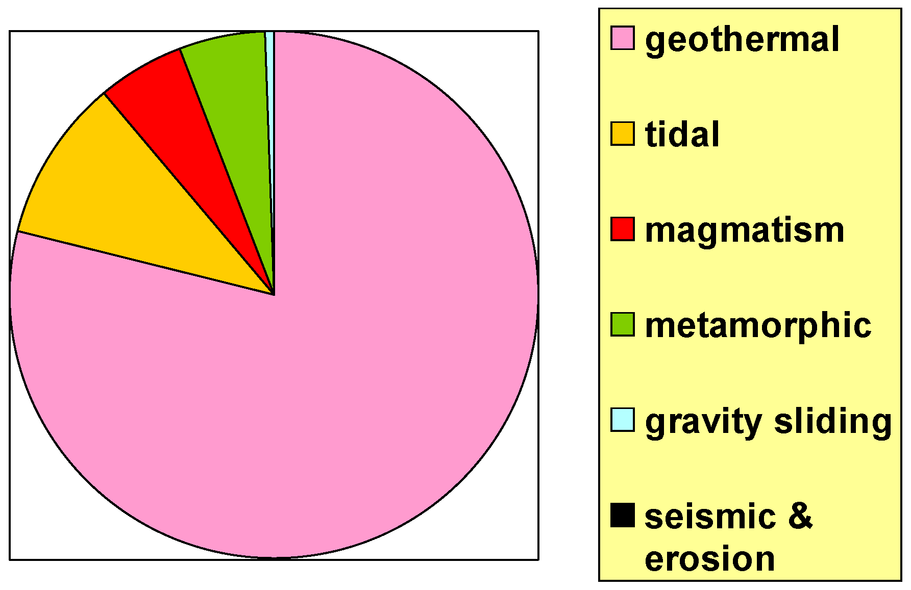
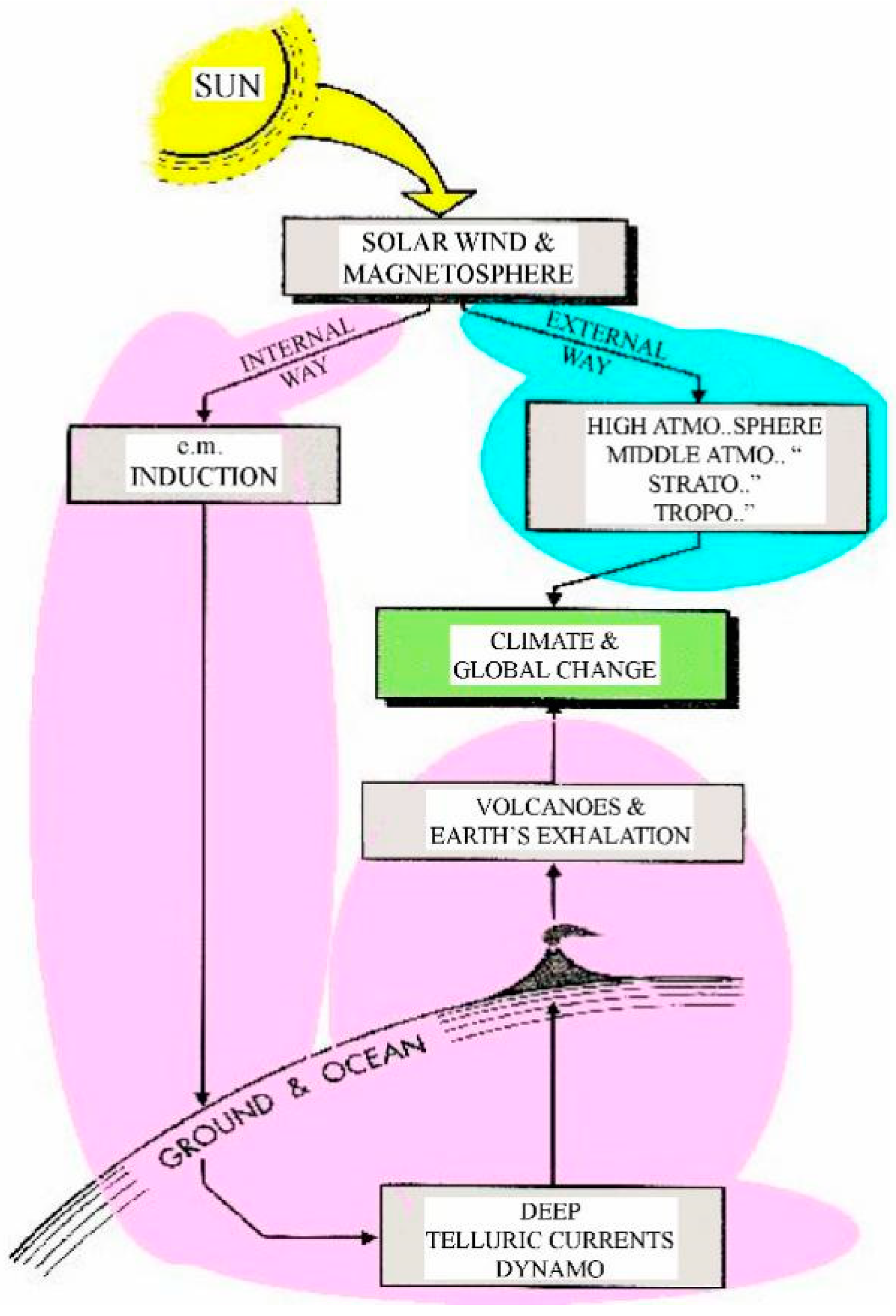
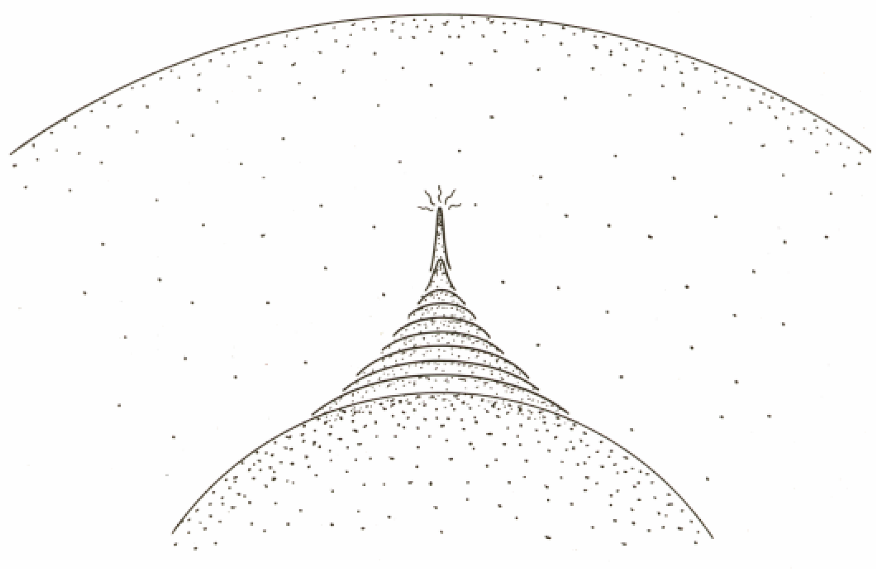
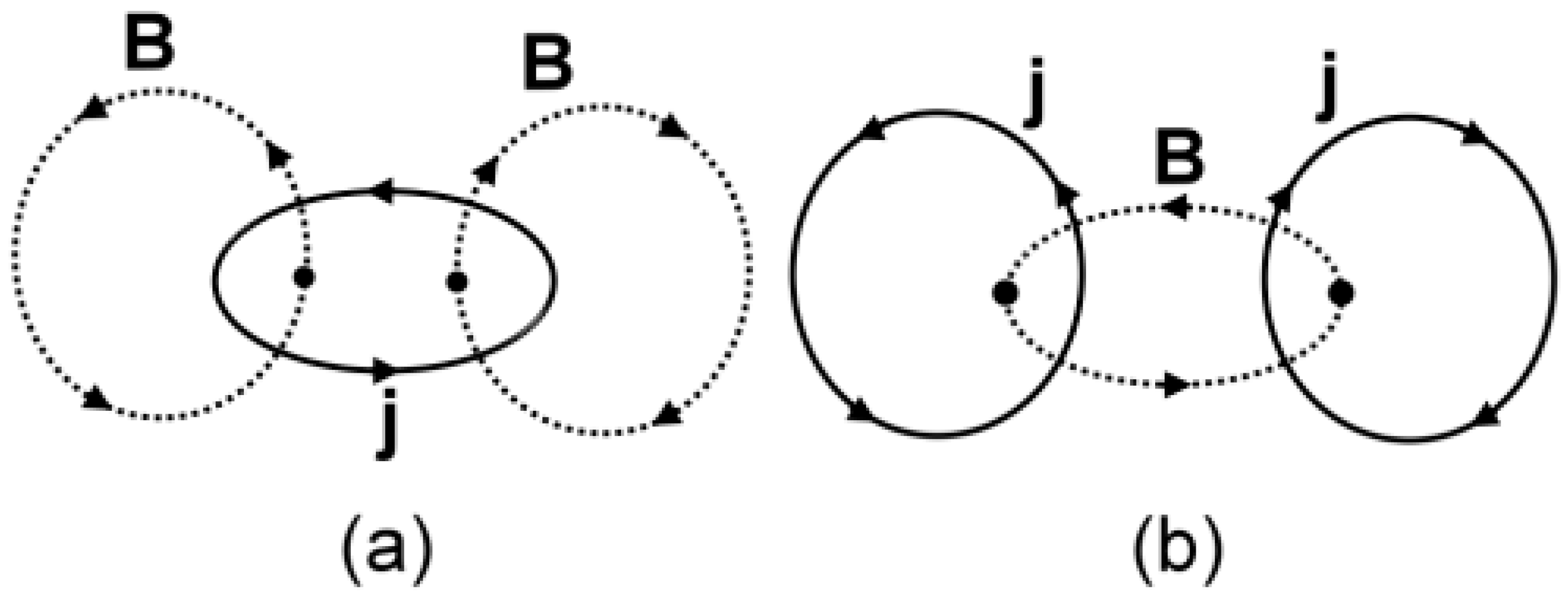
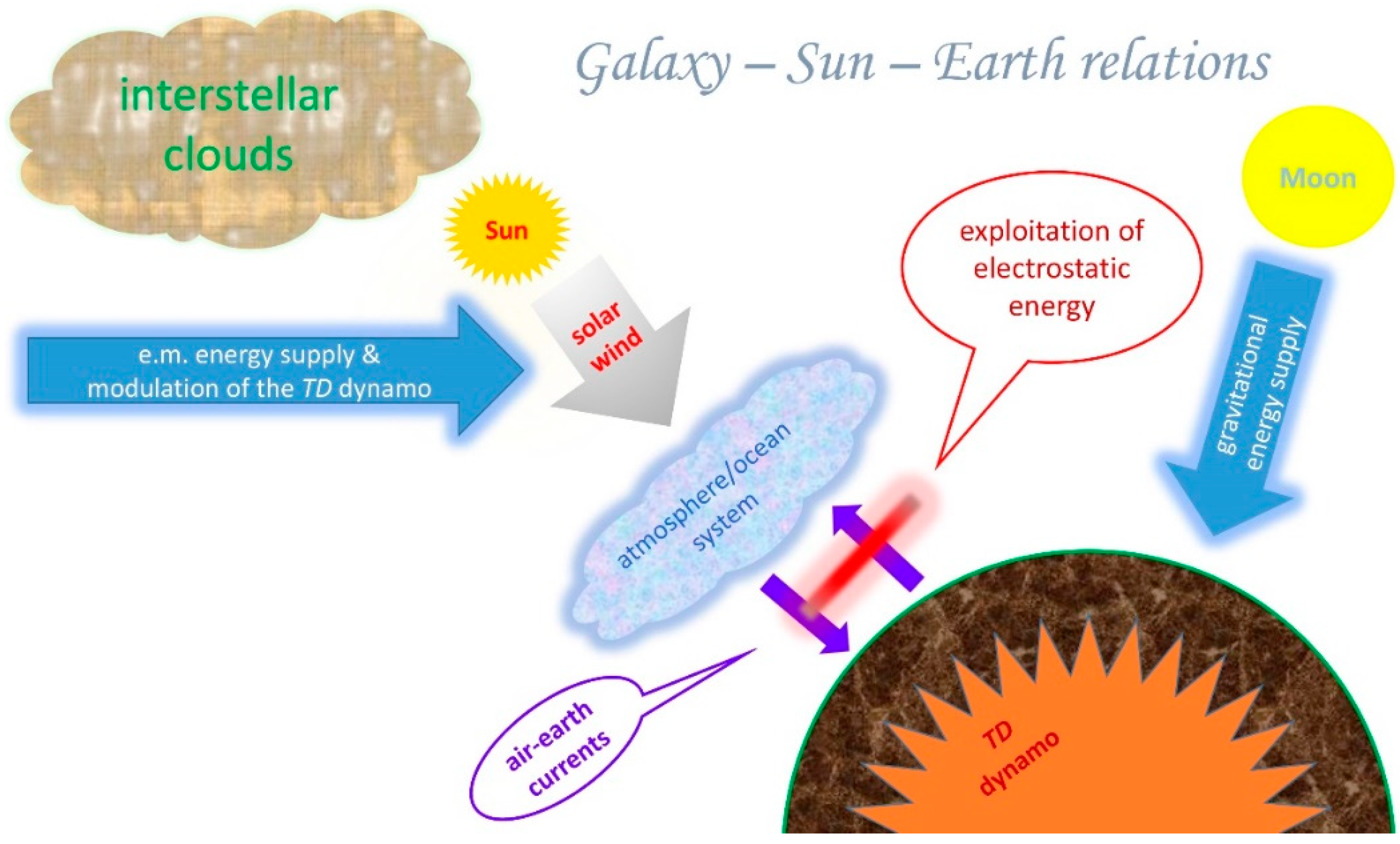
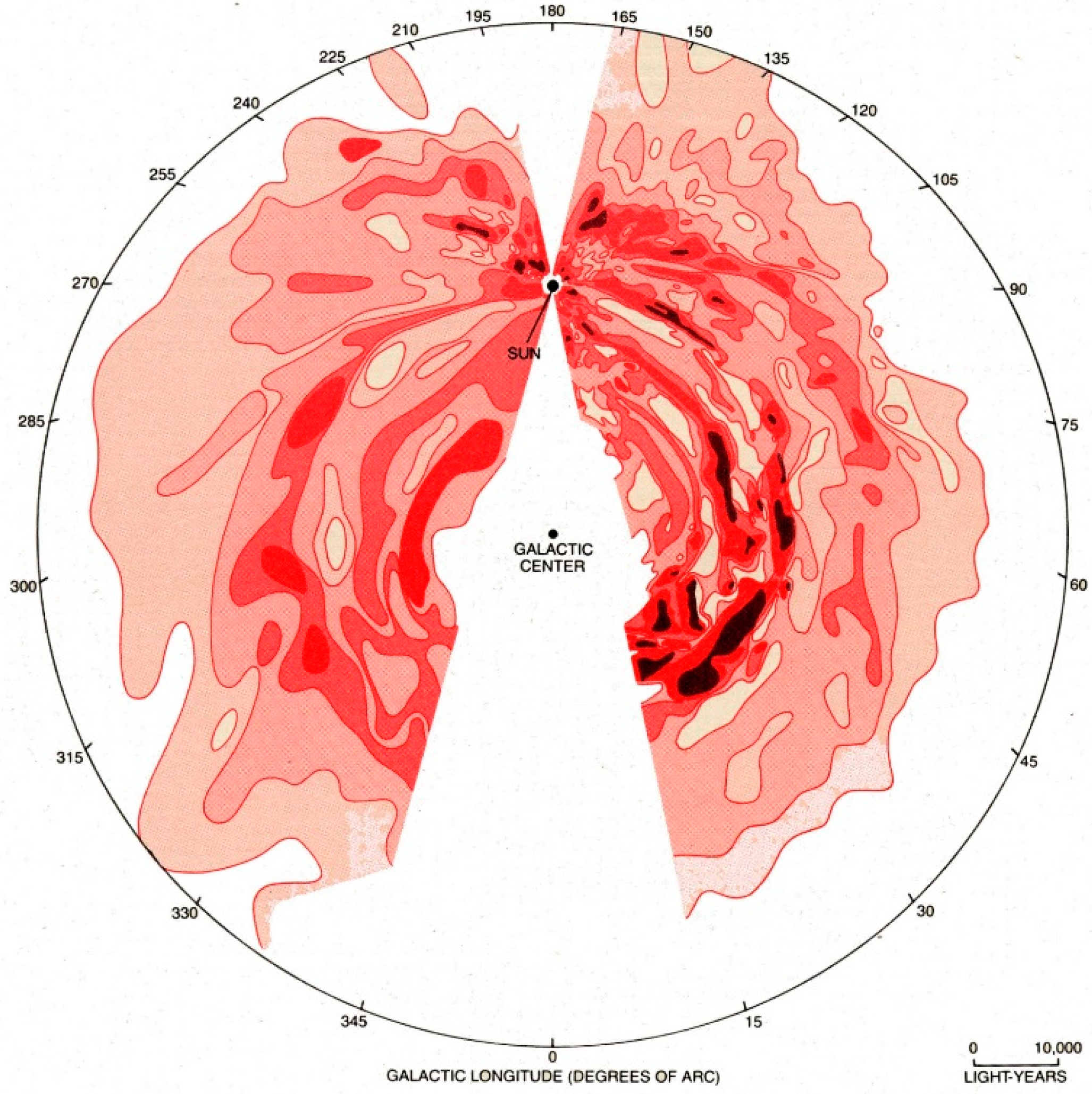
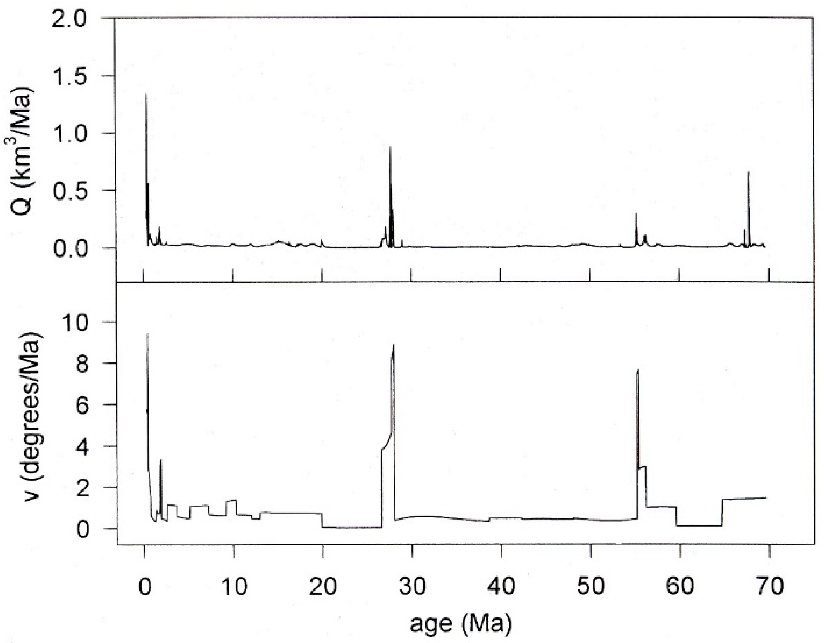
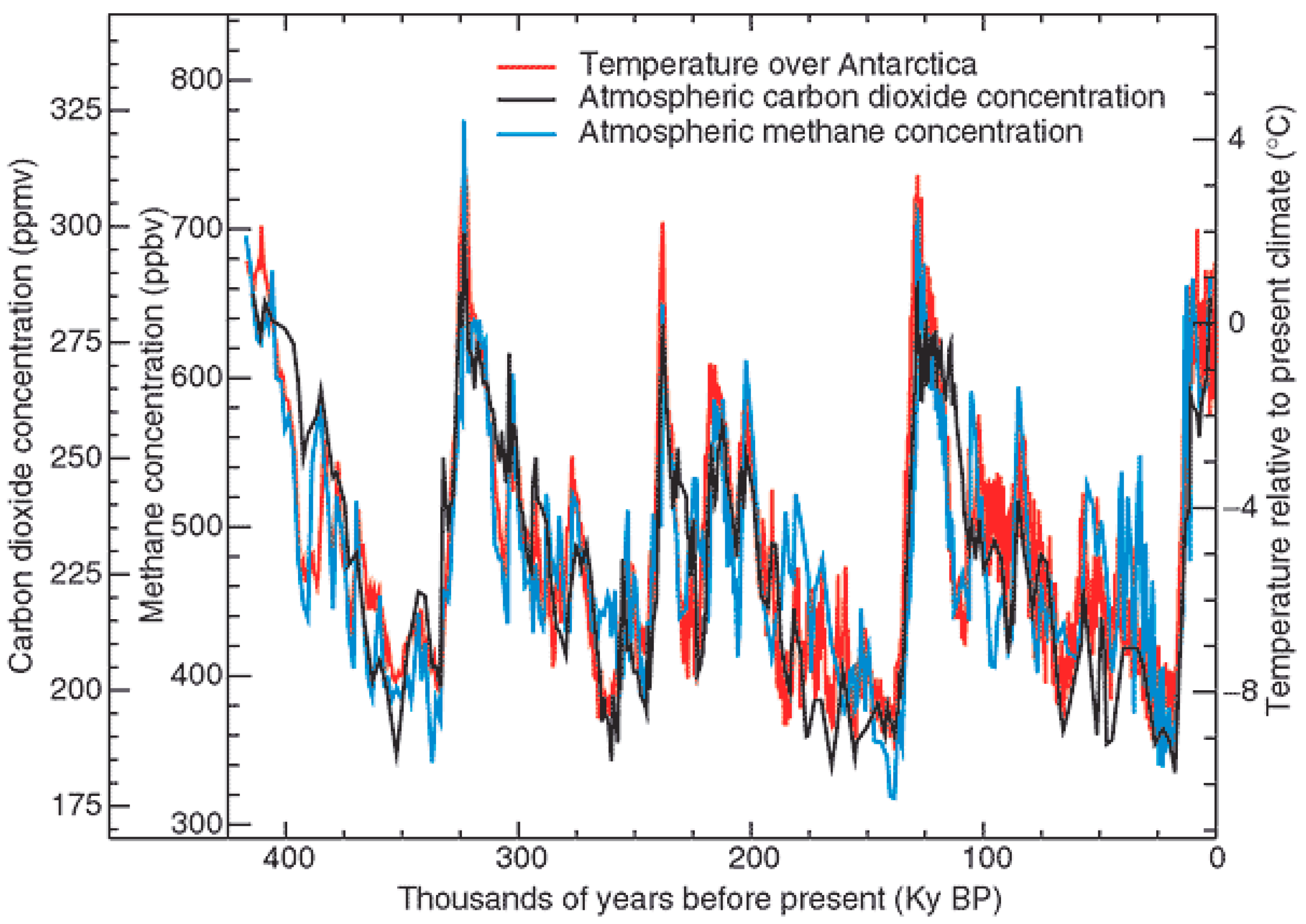
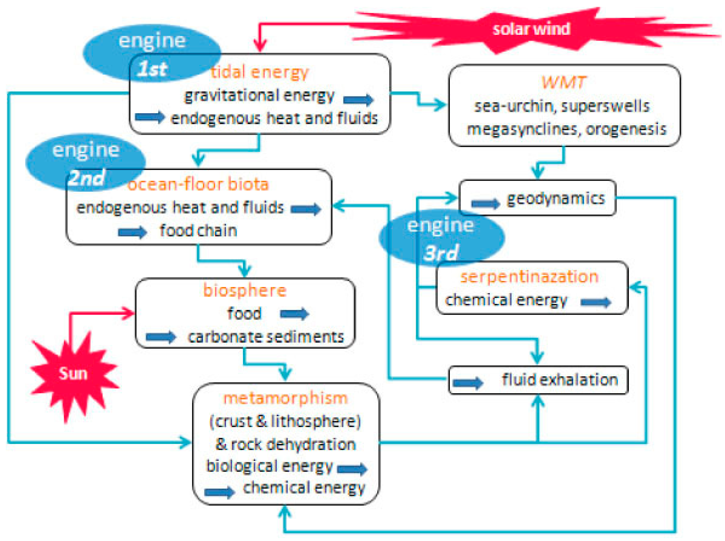
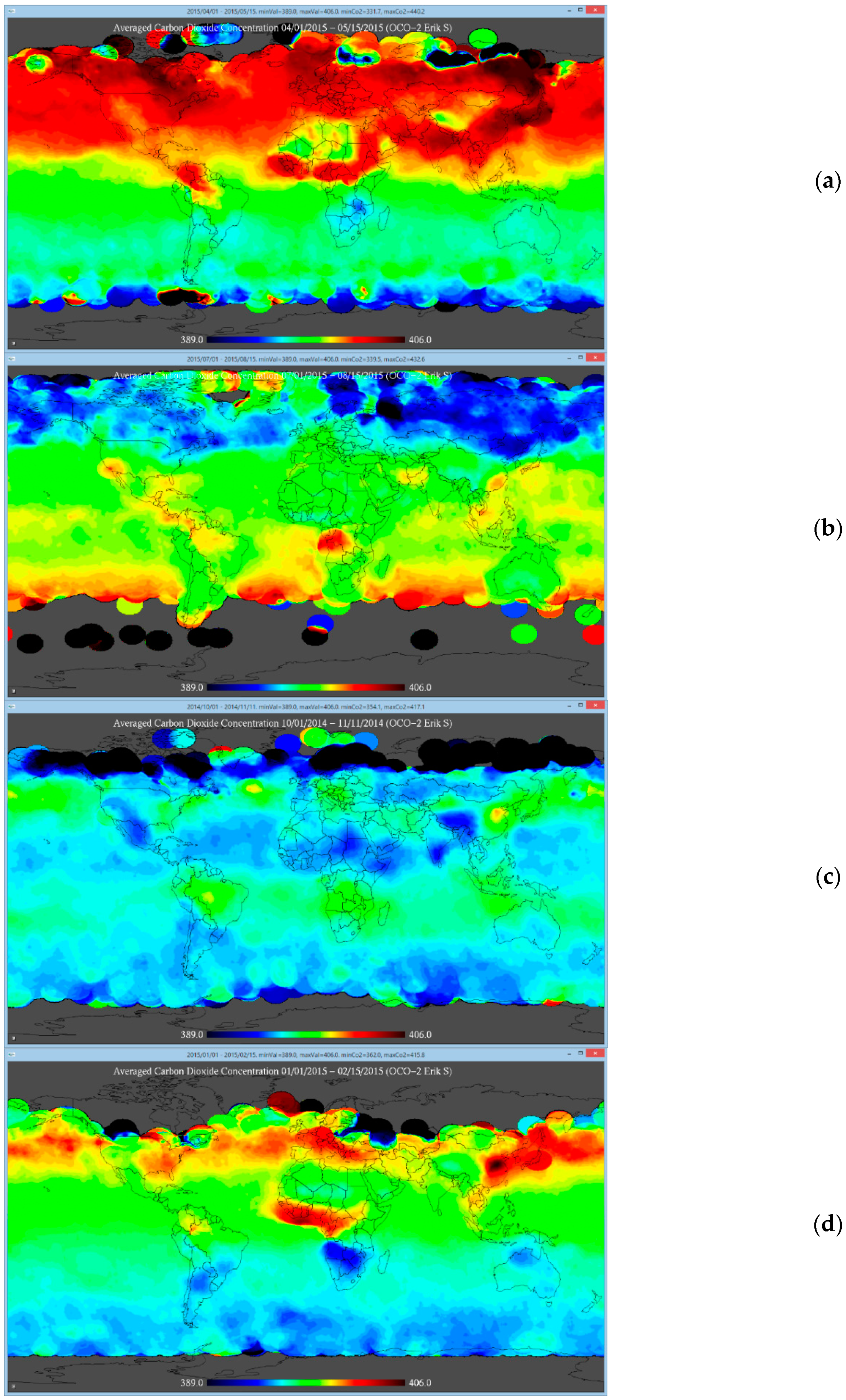
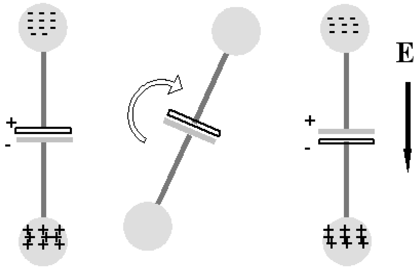
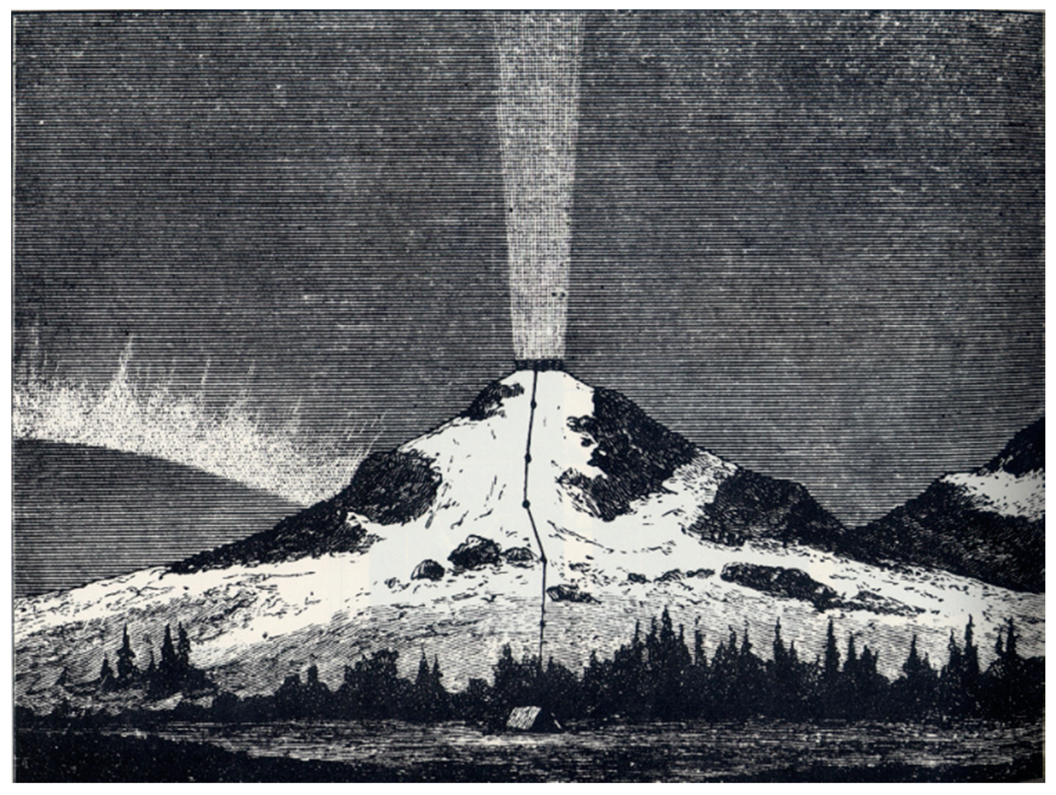
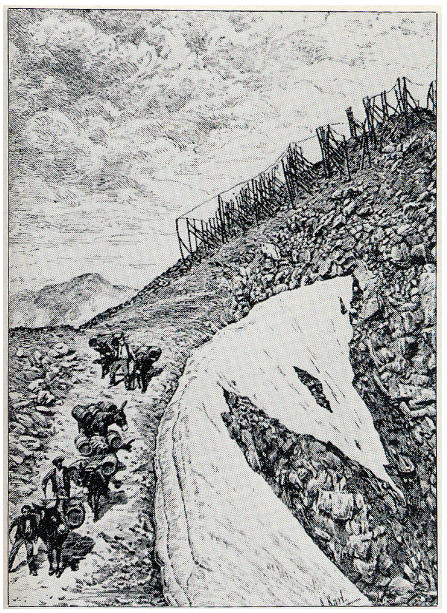
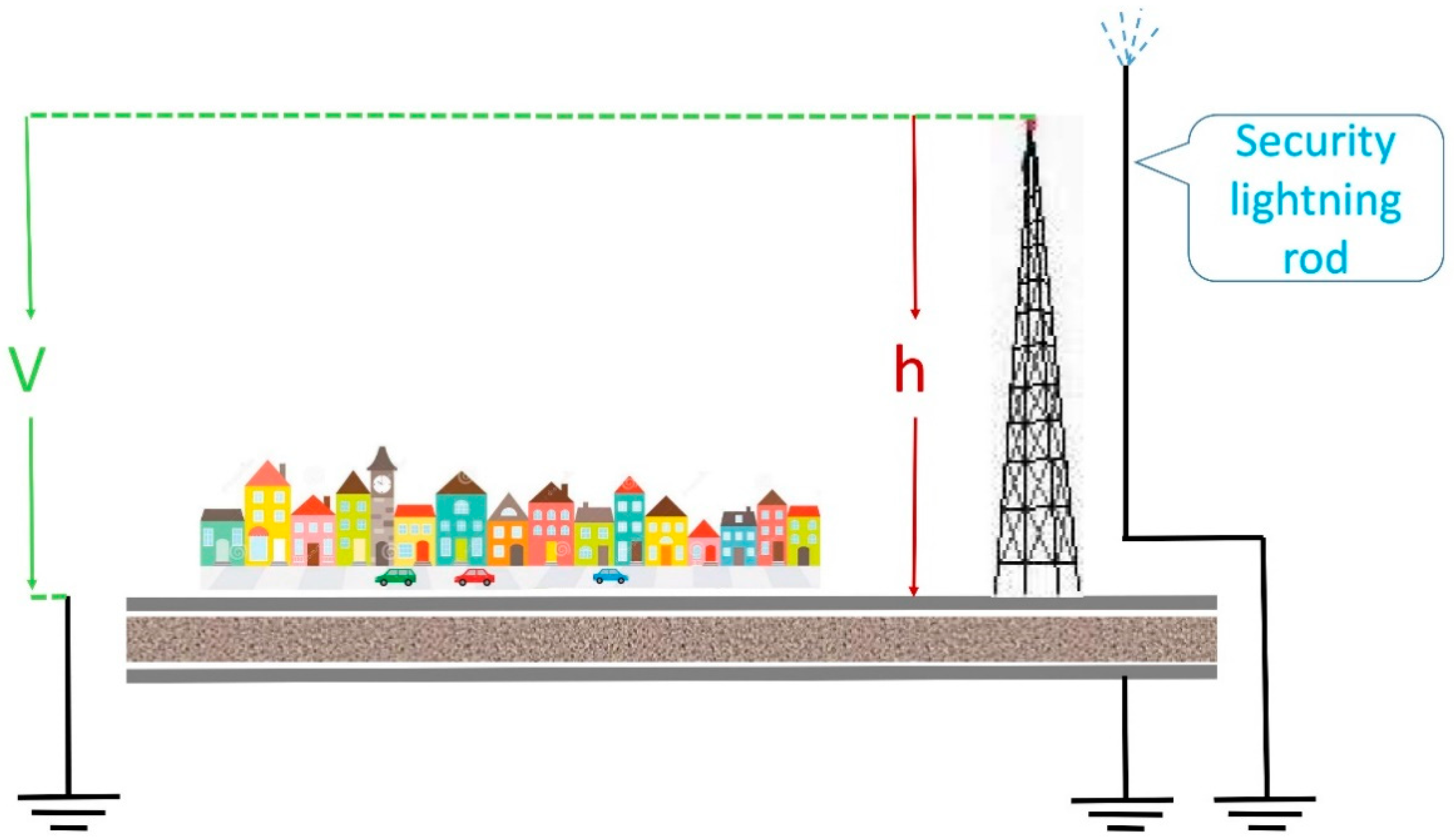
Table 1.
Endogenous energy of the Earth during the last few million years (×1013 W).
| Kind of Power | Estimate | Rough Value | Percent |
|---|---|---|---|
| global heat flow measured across Earth’s surface | 4.42 ± 0.10 | ~4.42 | ~79% |
| tidal friction (total) | 0.4 ÷ 0.7 | ~0.55 | ~10% |
| magmatic heat flux | 0.20 ÷ 0.39 | ~0.3 | ~5% |
| metamorphic heat for transforming sedimentary and volcanic rocks | the same order of magnitude | ~0.3 | ~5% |
| gravity sliding | 2.5 × 10⁻² | ~0.025 | ~0.5% |
| seismic | 0.3 ÷ 3 × 10⁻³ | ~0.5% | |
| potential energy loss due to soil erosion | 3 × 10⁻⁴ | ~0.0% | |
| Total | ~5.56 | 100% |
Table 2.
The principal parameters of a few components of the Earth.
| Total | Specific Heat | Thermal | |||
|---|---|---|---|---|---|
| parameter | thickness | mass | at constant | capacity | phase |
| (km) | (Kg) | pressure | ratio (c) | ||
| (J/g·K) | |||||
| atmosphere | 8 (a) | 5.3 × 10¹⁸ | 1.0 | 1 | gas |
| hydrosphere | 2.7 (b) | 1.4 × 10²¹ | 4.2 | 103 | liquid |
| cryosphere | 0.07 (b) | 3 × 10¹⁹ | 2.1 | 10 | solid |
(a) Scale height; (b) Average thickness when sea water is assumed to cover entire Earth with a uniform layer; (c) Ratio relative to atmosphere’s.
© 2020 by the author. Licensee MDPI, Basel, Switzerland. This article is an open access article distributed under the terms and conditions of the Creative Commons Attribution (CC BY) license (http://creativecommons.org/licenses/by/4.0/).
Share and Cite
MDPI and ACS Style
Gregori, G.P. Climate Change, Security, Sensors. Acoustics 2020, 2, 474-504. https://0-doi-org.brum.beds.ac.uk/10.3390/acoustics2030026
AMA Style
Gregori GP. Climate Change, Security, Sensors. Acoustics. 2020; 2(3):474-504. https://0-doi-org.brum.beds.ac.uk/10.3390/acoustics2030026
Chicago/Turabian StyleGregori, Giovanni P. 2020. "Climate Change, Security, Sensors" Acoustics 2, no. 3: 474-504. https://0-doi-org.brum.beds.ac.uk/10.3390/acoustics2030026