An Experimental and Numerical Study on the Effect of Spacing between Two Helmholtz Resonators

Abstract

This study investigates the acoustic performance of a system of two Helmholtz resonators experimentally and numerically. The distance between the Helmholtz resonators was varied to assess its effect on the acoustic performance of the system quantitatively. Experiments were performed using an impedance tube with two instrumented Helmholtz resonators and several microphones along the impedance tube. The relation between the noise attenuation performance of the system and the distance between two resonators is presented in terms of the transmission loss, transmission coefficient, and change in the sound pressure level along the tube. The underlying mechanisms of the spacing effect are further elaborated by studying pressure and the particle velocity fields in the resonators obtained through finite element analysis. The results showed that there might exist an optimum resonators spacing for achieving maximum transmission loss. However, the maximum transmission loss is not accompanied by the broadest bandwidth of attenuation. The pressure field and the sound pressure level spectra of the pressure field inside the resonators showed that the maximum transmission loss is achieved when the resonators are spaced half wavelength of the associated resonance frequency wavelength and resonate in-phase. To achieve sound attenuation over a broad frequency bandwidth, a resonator spacing of a quarter of the wavelength is required, in which case the two resonators operate out-of-phase.

1. Introduction

Broadband noise attenuation from aero-engines has become a challenging topic in the last decade for researchers from different backgrounds due to stringent noise emission regulations [1,2]. Expansions of airport operations have also been negatively affected due to these noise emission regulations [3]. Although there has been a significant reduction in aircraft noise emissions over the years, reducing it further through incremental changes is proving to be increasingly difficult [4]. The investigations for light-weight, space-efficient, broadband noise alternators span from the emerging field of acoustic meta-materials to Helmholtz resonators. A chronological summary of related past works in the field of aircraft noise reduction technologies was reported by Thomas et al. [5]. Acoustic liners are the most common sound attenuating devices employed in controlling aero-engine noise, and consist of a perforated face sheet enveloping a sequence of cavities, creating a series of Helmholtz resonators. These acoustic liners convert the incident acoustic energy into thermal energy as well as turbulent fluid motion due to the periodic inflow and outflow as the cavity resonates, or dissipates the acoustic energy by viscous forces [6].

A typical flight profile of an aircraft consists of various phases such as take-off, cruise, approach, and landing, all of which require different engine thrust settings. Varying the engine thrust setting leads to a change in parameters such as engine rpm, blade passing frequency, which would, in turn, change the bandwidth of frequencies to be absorbed in each particular flight phase [6]. Although Helmholtz resonators are efficient sound absorbing devices, they come with the penalty of being effective on a narrow band frequency range [6,7,8,9,10,11,12]. The efficiency of the Helmholtz resonator also depends on the sound pressure level of the incident acoustic field [13]. The sound absorption characteristics of a Helmholtz resonator are governed by various geometric factors, with the resonance frequency obtained using the classical lumped analysis,

$$f_o=\left(\frac{c_o}{2\pi }\right)\sqrt{\frac{S_n}{V_c(l_n+{\delta }_n)}},$$

(1)

where $c_0$ is the speed of sound, $S_n$ is the cross-sectional area of neck opening, $l_n$ is the length of the neck, $V_c$ is the volume of the cavity, and ${\delta }_n$ is the end correction factor which accounts for any discontinuities within the resonator leading to the creation of higher order modes [14,15,16]. Extensive research has been carried out to understand the effect of these geometric parameters on the sound absorption characteristics of a Helmholtz resonator. The effect of parameters related to the neck geometry such as the neck opening cross-sectional area, neck location and neck length for a resonator with circular and rectangular cavity was studied by Ingard [15]. The study developed end corrections to consider the excitation of higher order modes at the junction between the cavity and resonator neck. The effect of changing cavity depth and width for both a fixed and variable volume resonator was studied by Chanaud [16]. In this study, they showed that for a fixed resonator volume and neck parameters, the resonance frequency can be altered by changing the orifice shape. Moreover, they also showed that the orifice shape does not have a significant effect on the resonance frequency. The effect of cavity volume and orifice position was also studied by Dickey and Selamet [17], Selamet et al. [18] and Selamet and Ji [19]. These studies were focused on the effect of the resonator length on the transmission loss and resonance frequency as a function of its diameter.

Space constraints in the aerospace industry restrict the use of conventional single cavity Helmholtz resonators for low-frequency sound absorption. Selamet and Lee [20] studied the effect of increased neck length on the Helmholtz resonance behaviour. The study revealed that extending the neck into the cavity decreases the resonance frequency of the Helmholtz resonator without changing the overall volume of the cavity. The extended neck also acted similarly to a quarter wavelength resonator, thereby attenuating multiple higher frequencies as compared to a resonator without an extended neck. Cai et al. [21] took this study a step further by introducing a spiral neck to increase the effective neck length into the cavity, thereby further lowering the resonance frequency and keeping the cavity volume fixed. Multiple extended neck resonators within an acoustic liner would effectively attenuate a broad bandwidth of low-frequency aircraft noise.

Although there is a diverse range of literature on how a single resonator’s geometric parameters affect its sound absorption capability, the effect of spacing between consecutive resonators, within an acoustic liner assembly, remains to be investigated. Following on from the recent surge in resonator positioning optimization studies for broad bandwidth sound frequency attenuation, such as Coulon et al. [22], Cai et al. [23], and Wu et al. [24], the present work focuses on a detailed investigation into the effect of changing the spacing between two resonators and its impact on the transmission loss and transmission coefficient characteristics, as well as the change in sound pressure levels. An optimised resonator spacing, keeping the dimensions of the resonator fixed, might be beneficial in a range of sound reduction applications [25,26,27]. The paper is structured as follows: Section 2 provides a detailed description of the experimental methodology, test rig and numerical setup. Section 3 presents the numerical and experimental results along with a discussion of the findings, followed by Section 4, which concludes the manuscript.

2. Experimental, Analytical and Numerical Methodology

This section aims to provide a detailed description of the experimental facility, test rig, measurement techniques, analytical model and numerical methods employed in this study.

2.1. Testing Facility

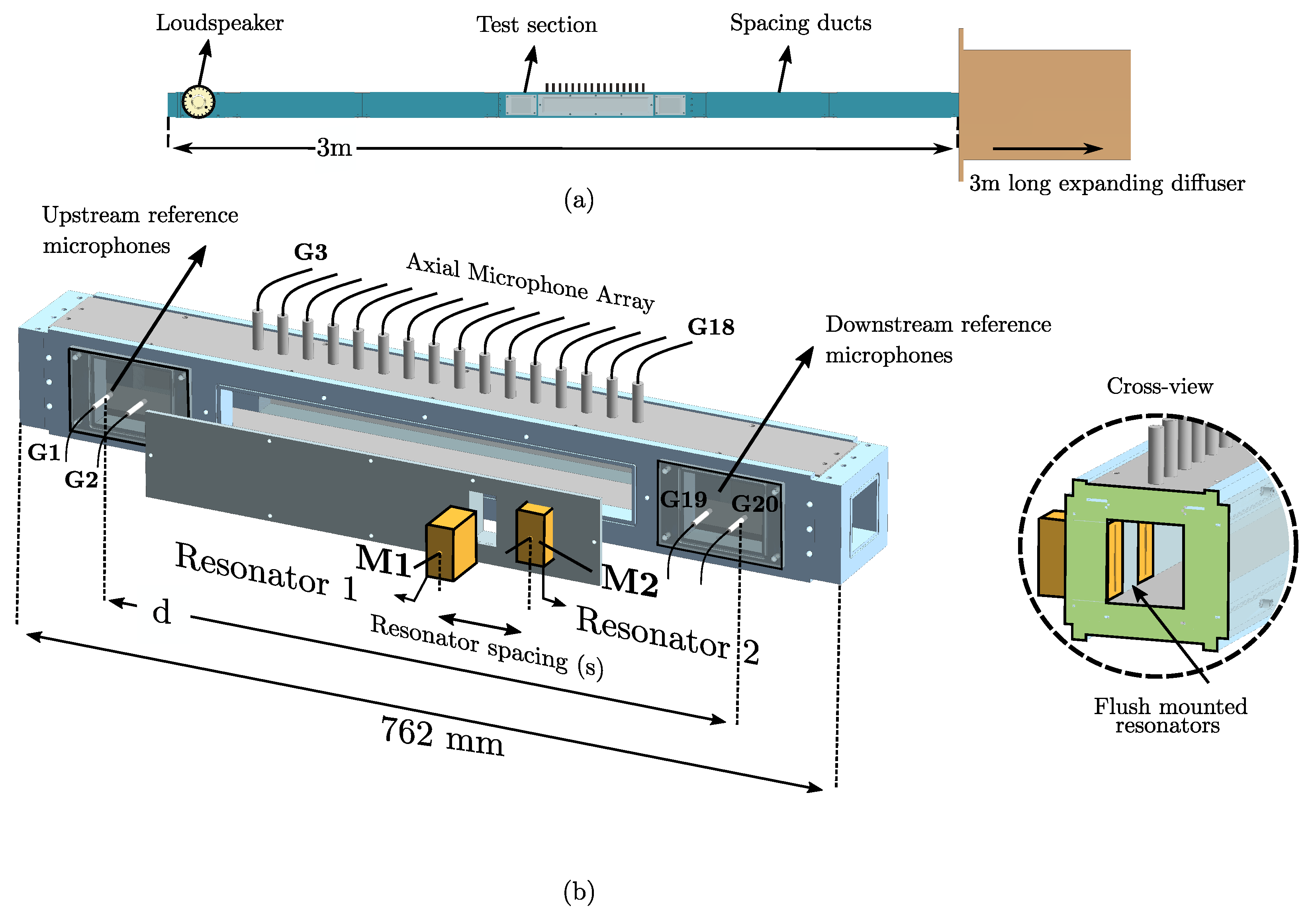
The experiments were performed at the University of Bristol Grazing Flow Impedance Tube Facility (UoB-GFIT). The schematic of the facility is presented in Figure 1a and a detailed view of the test section, along with the microphone naming convention is presented in Figure 1b. The impedance tube has a total length of 3000 mm, with a square cross section of 50.8 mm × 50.8 mm. The test section starts from 1180 mm downstream of the loudspeaker, which corresponds to 22 tube diameters, to ensure plane wave propagation. ASTM E2611-19 [28] suggests a minimum of three tube diameters to be allowed between the sound source and the nearest measuring microphone to ensure a plane wave in the test section. The test section had a length of 762 mm, shown in Figure 1b. The setup was designed to enable tests both with or without the presence of airflow. Although all experiments were conducted without airflow, when used with airflow, a 3000 mm long diffusing section can be added to the facility to reduce the air velocity at the exhaust and minimize acoustic reflections into the test section. The acoustic source used for the experiments consisted of two BMS 4592ND compression drivers, capable of generating sound pressure levels of up to 130 dB in the test section. The loudspeakers were excited at white noise with an amplitude of 10 V_pp using a Tektronix function generator. Noise data in the impedance tube was obtained using 20 G.R.A.S. 40 PL free-field array microphones. In addition, two FG-23329-P07 microphones were employed to obtain data about the internal pressure field of the resonators. The distance between the first and last microphones is denoted by “d”. The spacing between the microphones was determined by considering the frequency range of interest. The distance between the upstream microphones (G1 and G2) and downstream microphones (G19 and G20) was selected following the ASTM E2611-19 as [28],

$$\frac{0.01c_o}{f_l}<L<\frac{0.4c_o}{f_u},$$

(2)

where L is the spacing, $f_u$ and $f_l$ are the upper and lower frequency limits, respectively. These microphone couples were used to calculate the transmission loss and transmission coefficient, based on the standard test method for normal incidence determination of porous material acoustical properties based on the transfer matrix method, as outlined in ASTM E2611-19 [28]. The distance between the upstream microphones (G1 and G2) and downstream reference microphones (G19 and G20) had a 40 mm spacing, which allowed to capture sound waves accurately between 85 Hz and 3400 Hz. The axial microphone array (G3 to G18), which was used to address the change in the acoustic field along the impedance tube, was equally spaced at 25 mm over the test section (see Figure 1). These microphones were able to capture accurately the sound waves of frequencies between 137.5 Hz and 5488 Hz, which was well above the facilities’ cut-off frequency of 3375 Hz. Data collection was performed using a National Instruments PXIe-1082 data acquisition system, consisting of a PXIe-4499 sound and vibration module. Matlab R2016a was used to interface between the data acquisition system and the signal generator to run the data acquisition code.

2.2. Test Samples

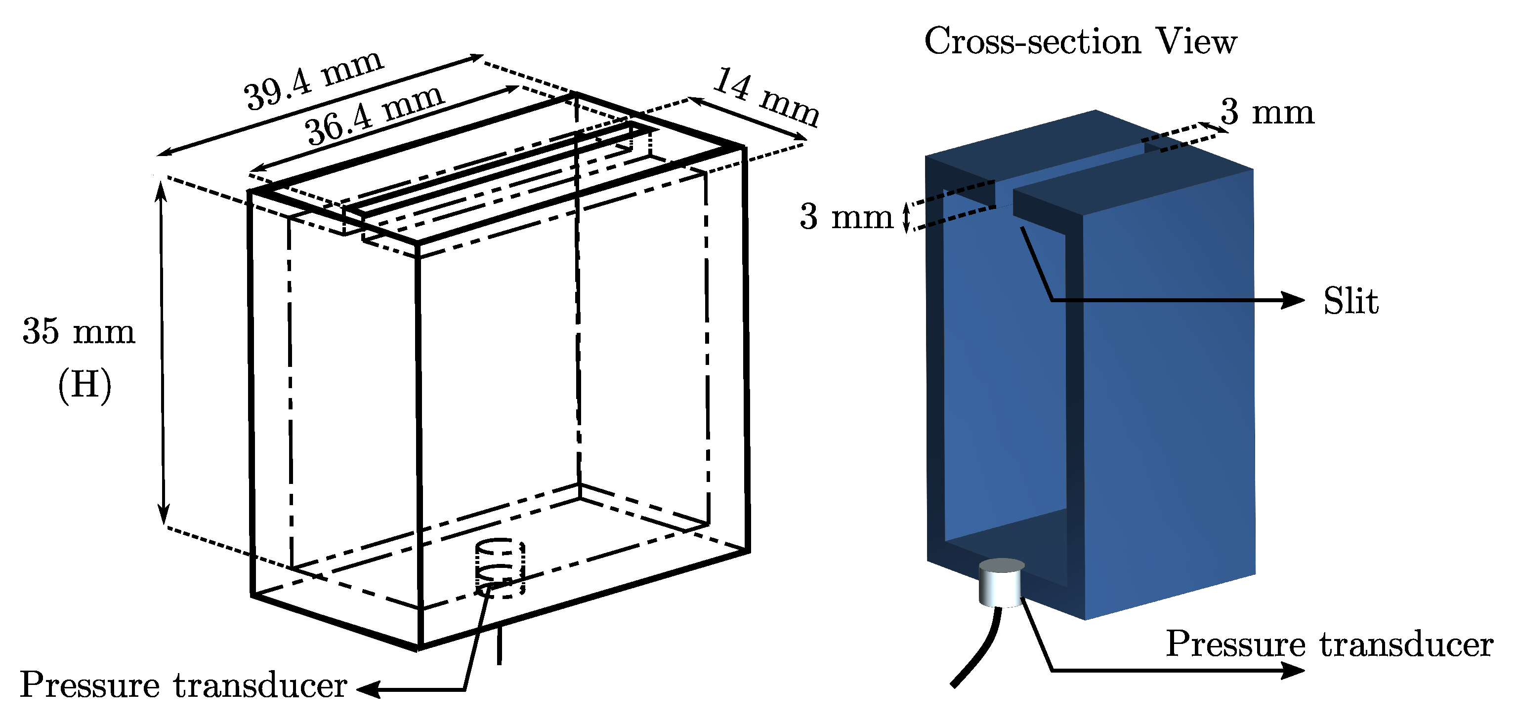
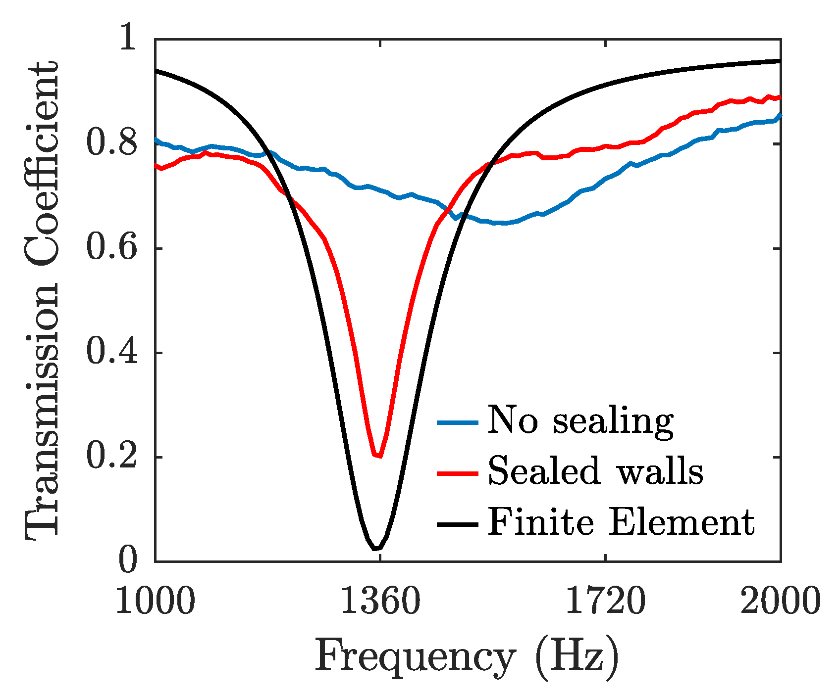
Two Helmholtz resonators, tuned to a resonance frequency of $f_o=1360$ Hz, were manufactured from 3 mm Perspex sheet. Figure 2 illustrates the geometrical details of the resonators used in this study. The perspex sheet was cut into designed dimensions of the resonator walls, which formed an internal cavity of dimensions of 36.4 mm × 35 mm × 14 mm. The neck length was 3 mm, and the slit opening dimensions were 36.4 mm × 3 mm. Knowles Omni-Directional (FG) 2.56 DIA electret condenser microphones (FG-23329-P07) were flush-mounted to the internal walls of both the resonators. These microphones were permanently glued to the resonator walls to obtain a perfect air seal and ensure accurate measurements. The microphones were calibrated in magnitude and phase prior to experiments using a reference G.R.A.S. 40PL free-field microphone with a known sensitivity value. The calibration procedure followed that outlined by Showkat [29]. The calibration results showed a phase shift of less than 7${}^{\circ }$ for a frequency range of 100 Hz to 3000 Hz, with a relatively constant amplitude sensitivity, not presented here for brevity. To ensure that the manufactured resonators resonated at their design frequency and were air-sealed perfectly, some preliminary tests were performed. The resonators were placed inside rectangular cut-outs within the test section side window, to obtain a flush mount with the internal walls, as shown in Figure 1b. Since the imperfections of the sealing of resonators can lead to a shift in the resonance frequency of the resonators [30], the transmission coefficient induced by a single resonator was measured and studied. Figure 3 shows the transmission coefficient induced in the system by two different resonator sealing configurations in comparison with the results obtained from the numerical simulation. The details of the calculations are presented in Section 3. The results suggest that the resonator does not perform well in the absence of a proper sealing, leading to a shift in the resonance frequency and weaker sound attenuation. However, by employing a proper sealing, the resonator performs as expected at its design frequency of $f_o=1360$ Hz, which is evident by the prominent dip in the transmission coefficient behaviour. Besides, the experimental results show a good agreement with the results obtained using Finite Element Analysis, with only a slight difference in the magnitude. This difference may be culminated due to the subtle differences in boundary conditions, such as hard-wall assumption.

2.3. Experimental Approach

The two Helmholtz resonators were flush-mounted to the internal wall of the impedance tube working section. A total of 22 microphones were employed to obtain data from the impedance tube test section and resonators. The experiments were performed at a sampling rate of 2¹⁵ Hz for 16 s. The two upstream and downstream microphones (see Figure 1) were used to calculate the transmission loss and transmission coefficient, based on the standard test method for normal incidence determination of porous material acoustical properties based on the transfer matrix method, as outlined in ASTM E2611-19 [28]. The array of 16 microphones (G3–G18) were used to quantify the change in sound pressure level in the impedance tube test section.The FG-23329-P07 microphones M1 and M2, were employed to obtain data about the internal pressure field of the resonators. In order to have a clear understanding of the effect of resonator spacing on the sound field in the impedance tube, thirteen different resonators spacing configurations, spanning $0.13<s/\lambda <1$, were investigated experimentally, where s is the spacing between the two resonators, as shown in Figure 1. Hereafter, to ease the interpretation of the results, the spacing between the resonators are non-dimensionalized with the wavelength ($\lambda$) of the target resonance frequency ($f_o$), i.e., $s/\lambda$.

The frequency–energy content of the acoustic pressure was presented in terms of the sound pressure levels (SPL). The SPL was calculated as,

$$\begin{array}{c}\hfill \mathit{SPL}\left(\mathit{f}\right)=10lo{g}_{10}\left(\frac{p^2\left(f\right)}{p_o^2}\right),\end{array}$$

(3)

where $p\left(f\right)$ is the frequency dependent pressure fluctuations calculated from microphone signals and $p_o$ is the reference pressure (20 $\mathsf{\mu }$Pa). The PSD of the pressure fluctuations, which was used to obtain frequency-dependent pressure values, was estimated by using the Welch method [31], where the data from the transducers are segmented in 32 equal lengths with 50% overlap and windowed by the Hamming function, and the resulting spectrum had a frequency resolution of 16 Hz.

2.4. Analytical Model

The analytical model in this study was adopted from [7], and the results from the analytical model is compared with the experimental and numerical results. A detailed version of the derivation of transmission loss for lined Helmholtz resonator array can be found in [7]. A classical lumped approached was adopted to model a Helmholtz resonator mounted to the side of a duct. An end correction factor was introduced to consider any higher order modes and improve the accuracy of the model. The acoustic impedance of a single Helmholtz resonator is given by,

$$\begin{array}{c}\hfill {\mathit{Z}}_r=j\frac{{\rho }_0{l}_n^{\prime }}{A_n\omega }({\omega }^2-{\omega }_0^2),\end{array}$$

(4)

where ${\rho }_0$ is the density of air, $A_n$ is the area of the connecting neck and $l_n^{\prime }$ is the effective neck length, calculated through correction methods [16] from the original neck length $l_n$. Here, $\omega$ is the angular frequency and ${\omega }_0$ is the resonant angular frequency of the Helmholtz resonator, given by

$${\omega }_0=c_0\sqrt{\frac{A_n}{l_n{V}_c}},$$

(5)

where $V_c$ is the volume of the resonating cavity. The transmission loss of a single resonator mounted on a duct with cross-sectional area $A_d$ can be calculated, once the impedance $Z_r$ is known, using

$$\begin{array}{c}\hfill TL=20{log}_{10}\left(\frac{1}{2}\left|2+\frac{{\rho }_0{c}_0}{A_d}\frac{1}{Z_r}\right|\right).\end{array}$$

(6)

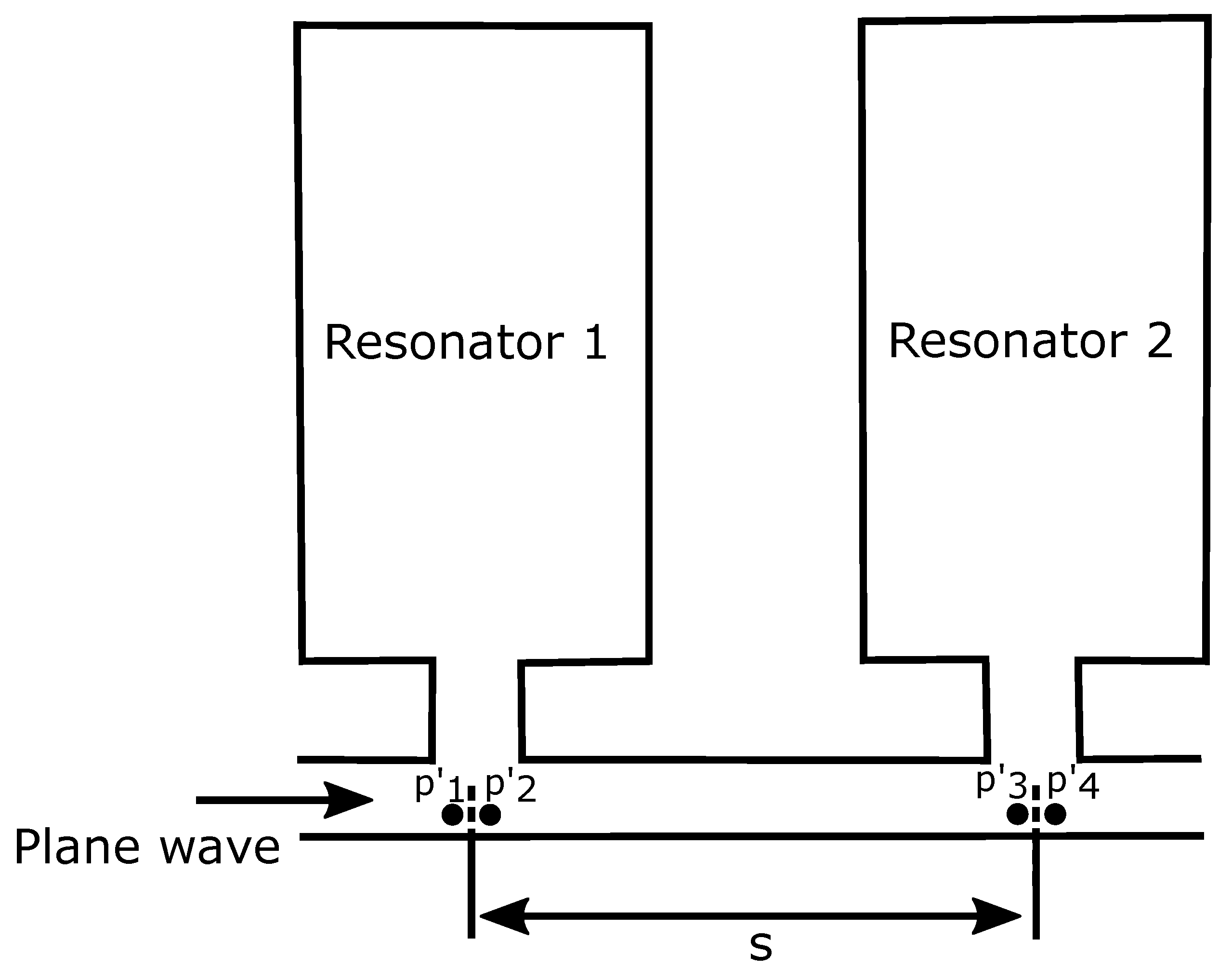
For a two resonator system lined on a duct, the following continuity conditions for the acoustic pressure and particle velocity can be expressed at the four locations shown in Figure 4 [7],

$$\begin{array}{c}\hfill {\mathit{p}}_1^{\prime }=p_2^{\prime },p_3^{\prime }=p_4^{\prime },\end{array}$$

(7)

$$\begin{array}{c}\hfill {\mathit{u}}_1{A}_d=\frac{p_2^{\prime }}{Z_{r1}}+u_2{A}_d,u_3{A}_d=\frac{p_4^{\prime }}{Z_{r2}}+u_4{A}_d,\end{array}$$

(8)

where $Z_{r1}$ and $Z_{r2}$ are acoustic impedance values of the two resonators. Combining the continuity conditions of pressure and velocity yields to the relations,

$$\begin{array}{c}\left[\begin{array}{c}{p}_1^{\prime }\\ {\rho }_0{c}_0{u}_1\end{array}\right]=\left(\begin{array}{cc}1& 0\\ \frac{{\rho }_0{c}_0}{A_d}\frac{1}{Z_{r1}}& 1\end{array}\right)\left[\begin{array}{c}{p}_2^{\prime }\\ {\rho }_0{c}_0{u}_2\end{array}\right]=T_{r1}\left[\begin{array}{c}{p}_2^{\prime }\\ {\rho }_0{c}_0{u}_2\end{array}\right],\end{array}$$

(9)

$$\begin{array}{c}\left[\begin{array}{c}{p}_3^{\prime }\\ {\rho }_0{c}_0{u}_3\end{array}\right]=\left(\begin{array}{cc}1& 0\\ \frac{{\rho }_0{c}_0}{A_d}\frac{1}{Z_{r2}}& 1\end{array}\right)\left[\begin{array}{c}{p}_4^{\prime }\\ {\rho }_0{c}_0{u}_4\end{array}\right]=T_{r2}\left[\begin{array}{c}{p}_4^{\prime }\\ {\rho }_0{c}_0{u}_4\end{array}\right].\end{array}$$

(10)

Assuming the propagation of planar wave only, the duct can be described by a transmission matrix [32]. By considering the delay of planar wave travelling between points 2 and 3, the duct transmission matrix can be defined as,

$$\begin{array}{c}\left[\begin{array}{c}{p}_2^{\prime }\\ {\rho }_0{c}_0{u}_2\end{array}\right]=\left(\begin{array}{cc}cos\left(ks\right)& jsin\left(ks\right)\\ jsin\left(ks\right)& cos\left(ks\right)\end{array}\right)\left[\begin{array}{c}{p}_3^{\prime }\\ {\rho }_0{c}_0{u}_3\end{array}\right]=T_{duct}\left[\begin{array}{c}{p}_3^{\prime }\\ {\rho }_0{c}_0{u}_3\end{array}\right],\end{array}$$

(11)

where k is the wave number and s is the spacing between two resonators. After obtaining the relations for the pressure and velocity values for consecutive points along the duct, the overall transfer equation relating $p_1^{\prime }$ to $p_4^{\prime }$ can be found from,

$$\begin{array}{c}\left[\begin{array}{c}{p}_1^{\prime }\\ {\rho }_0{c}_0{u}_1\end{array}\right]=T_{r1}{T}_{duct}{T}_{r2}\left[\begin{array}{cc}{t}_{11}& t_{12}\\ t_{21}& t_{22}\end{array}\right]\left[\begin{array}{c}{p}_4^{\prime }\\ {\rho }_0{c}_0{u}_4\end{array}\right],\end{array}$$

(12)

where the terms in the overall transfer matrix $t_{11}$, $t_{12}$, $t_{21}$ and $t_{22}$, can be used to calculate the transmission loss through Equation (12) [32],

$$\begin{array}{c}\hfill \mathit{T}L=20lo{g}_{10}\left(\frac{1}{2}|t_{11}+t_{12}+t_{21}+t_{22}|\right),\end{array}$$

(13)

Finally, the transmission coefficient, $TC$, defined as the ratio of the terminal acoustic power ($P_{out}$) and the input acoustic power ($P_{in}$), can be found from,

$$\begin{array}{c}\hfill \mathit{T}C=\frac{P_{out}}{P_{in}}=\frac{2}{t_{11}+t_{12}+t_{21}+t_{22}}.\end{array}$$

(14)

2.5. Numerical Simulations

Finite element analysis simulations were performed using the commercial software, COMSOL Multiphysics [31], to obtain the acoustic domain information and to calculate transmission coefficient and transmission loss for the different Helmholtz resonator spacing configurations. The simulations were carried out to model the experimental tests to a level of accuracy such that the simulation results can be confidently used to further visualise and analyse the acoustic field, both in the impedance tube and inside the resonators. In order to achieve a better representation of the physical phenomenon, the acoustic domain was separated into two regions: a lossless pressure acoustics model was applied to the domains before and after the resonator region, and a thermo-viscous model was applied to the domain where the resonators were present, to accurately model the thermal and viscous boundary layers existing in geometries with small dimensions, such as the resonator neck. Both the pressure acoustics and thermoviscous acoustics domain were coupled through the multiphysics coupling capability of the software.

The physics interface solves the Helmholtz equation, when using the lossless pressure acoustics, frequency domain interface. While using the thermo-viscous acoustics, frequency domain interface, it is necessary for the governing equations to explicitly include the thermal conduction effects and losses due to viscosity. Therefore, full linearized Navier–Stokes, continuity and energy equations are solved simultaneously for the domain with the thermo-viscous acoustics model. Solving the Helmholtz equations in the lossless pressure acoustics domain, requires only one time scale, T, which is the period of the incoming acoustic wave. However, there exists several length scales, namely the wavelength ($\lambda$), the mesh size, the acoustic boundary layer thickness and the smallest geometric dimension in the domain. The quality of the mesh is governed by its ability to resolve both the wavelength and the smallest geometric features [33]. In order to sufficient spatial resolution, the maximum mesh element size should be less that $\lambda /N$ where N is a number between 5 and 10 which depends on the spatial discretization [33]. The mesh for the steady numerical simulations was a free triangular mesh to resolve the impedance tube domain, and a boundary layer mesh for the regions where thermo-viscous acoustics model was implemented. A boundary layer mesh consists of a structured dense element distribution in the normal direction along specific boundaries. A mesh refinement study was conducted and the results for simulations based on the maximum mesh element of size $\lambda /3$ to $\lambda /60$ were compared. Based on the results, the mesh with maximum element size of $\lambda /6$ was employed, where $\lambda$ represents the wavelength of the corresponding highest frequency of interest (cut-off frequency of the duct), i.e., 3000 Hz. The minimum element size was 1/10th of the wavelength of the highest frequency of interest. In addition, the mesh around the neck was refined to have a sufficient resolution. The maximum element growth rate was 1.2 with a curvature factor of 0.3, and resolution of narrow regions, which controls the number of layers in the narrow regions, was set to a value of 3. The mesh for the pressure acoustics domain had Quadratic-Lagrange type element order, whereas the mesh for the thermoviscous domain was built with linear element order for pressure and Quadratic Lagrange element order for the velocity and temperature.

A port boundary condition was used to set up an incident wave at the upstream boundary to model a source and prescribe a non-reflecting condition at the end of the waveguide, i.e., an acoustic termination. The acoustic transmission loss in the simulation domain was calculated as,

$$\mathit{TL}=10lo{g}_{10}(\frac{W_{in}}{W_{out}}),$$

(15)

where

$$\begin{array}{c}\hfill {\mathit{W}}_{\mathit{in}}={\int }_{S_{in}}\frac{p_{o,s}^2}{\rho c_0}ds,\\ \hfill {\mathit{W}}_{\mathit{out}}={\int }_{S_{out}}\frac{\mid p^2\mid }{\rho c_0}ds,\end{array}$$

(16)

in which $c_0$ is the speed of sound (343 m/s), $\rho$ is the density of air (1.173 kg/m${}^3$), p is the estimated pressure value, $p_0,s$ is the inlet pressure (1 Pa), and $W_{in}$ and $W_{out}$ represent the inlet and outlet total acoustic power values calculated over the inlet and outlet port areas $S_{in}$ and $S_{out}$, respectively.

For the transient simulations, the transient pressure acoustics model was applied to the entire impedance tube apart from the region consisting the Helmholtz resonator, where a transient thermo-viscous model was applied. The mesh type, size and element order was same as the steady simulations. An incident pressure plane wave was modelled by adding a background pressure field node, with an initial pressure amplitude $p_o$ of 1 Pa. A perfectly matched layer (PML) was added on either side of the impedance tube to model an anechoic termination on both ends of the impedance tube, preventing data contamination due to any acoustic reflections. Transient simulations consist of two different time scales, i.e., the one given by the frequency of the incoming pressure wave and another one governing the size of the time step used by the numerical solver. The generalised alpha method was used for time stepping. The study was carried out at the designed resonant frequency of the Helmholtz resonator ($f_o$), with the simulation being run for 30 time-periods ($T_o$), to achieve convergence in results. The time step was chosen to be $T_o/60$. Pressure and particle velocity data were acquired through 50 domain probe points inside each of the resonator cavities, along the length of the resonator. The domain probe points were spaced 1 mm apart, with the first point being 12 mm below the resonator opening.

3. Results and Discussion

The results presented in this study explore the effect of resonators spacings on the sound attenuation performance of a two Helmholtz resonator system. The effect of the second resonator and the importance of its location is prevailed by presenting the results of the transmission coefficient and the transmission loss. In addition, a detailed analysis of the acoustic field (pressure and velocity field) both inside the impedance tube and the resonator cavities are presented to elaborate the effect of the spacing between the resonators on the overall performance of the system.

3.1. Acoustic Behaviour of a Two Resonator System

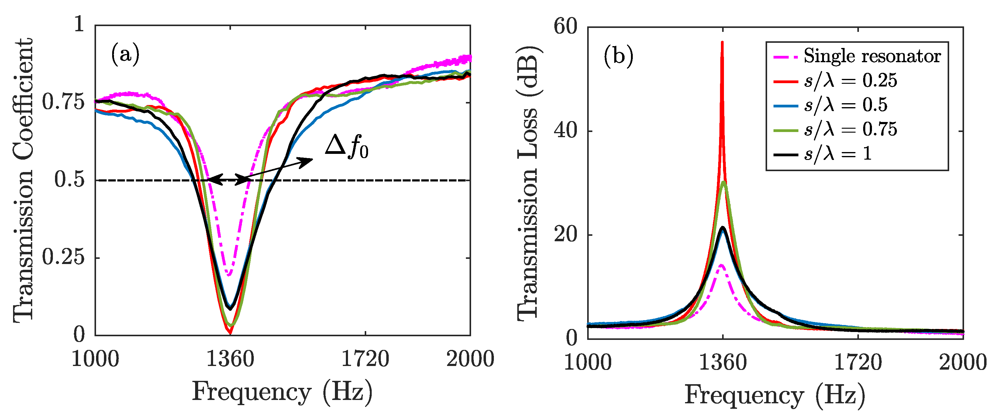
A conventional aircraft acoustic liner consists of multiple resonating cavities. An understanding of optimised distribution may be exploited to maximise the acoustic performance and allow tailoring for targeted frequencies. The addition of multiple resonators in a duct has been known to have a complex effect on the sound field [23]. To understand the complex nature of resonators interaction within an acoustic liner and its effect on the sound field, a simplified study has been defined using two resonators to characterise the interaction of two resonating cavities separated by a defined distance. Figure 5 presents the transmission coefficient and transmission loss characteristics of a two resonator system in comparison with a single Helmholtz resonator, with resonator spacings of $0.25<s/\lambda <1$. Figure 5a presents the transmission coefficient, which can be described as the ratio of the transmitted sound power to the incident sound power, and may shed light on the range of frequencies attenuated by an acoustic treatment. The range of frequencies attenuated by the resonators was estimated at a transmission coefficient of 0.5 and was defined as $\Delta f$, as shown in Figure 5. To further elaborate on the effect of the resonators’ separation distance on the acoustic behaviour, acoustic transmission loss, which is a measure of the magnitude of sound attenuated (in dB), is presented in Figure 5b. Considering the results for a single resonator, the transmission coefficient exhibits a dip at around $f=1360$ Hz, as expected. In addition, the transmission loss exhibits a peak at around the same frequency. The results presented in Figure 5 reveal that introducing a second resonator has a considerable effect on both transmission loss and coefficient. The transmission coefficient results in Figure 5a show that the attenuated frequency range increases for all the separation distances compared to the single resonator results. Moreover, for $s/\lambda =0.5$, $\Delta f$ peaks and is 104% (114 Hz) larger than the single resonator case, whereas the transmission loss for $s/\lambda =0.25$ is 302% (42 dB) higher than a single resonator case. The results indicate that the distance between the resonators may lead to unexpected acoustic behaviours, which need further analyses to prevail the underlying mechanisms.

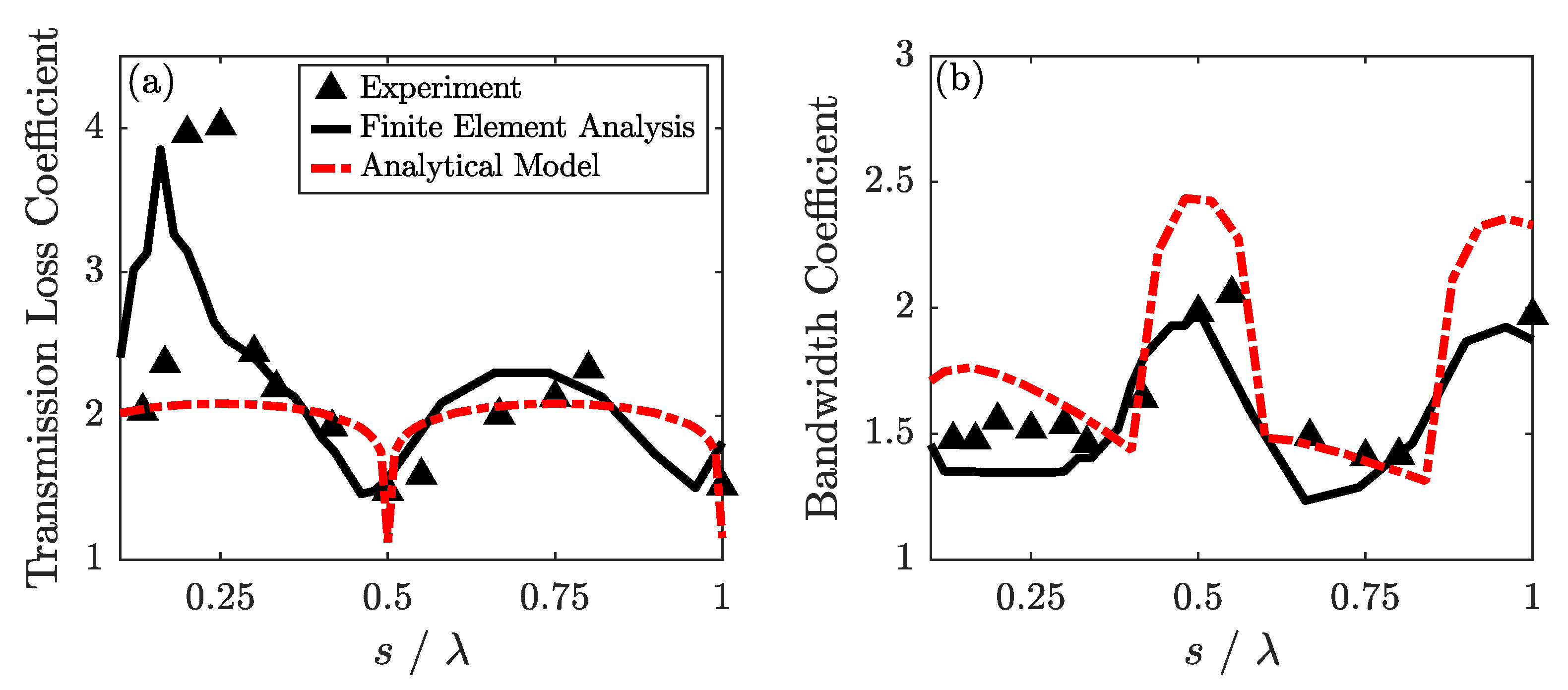
Figure 6 is constructed to gain a better understanding of the effect of the spacing on the sound attenuation performance induced by a two resonator system. Figure 6a presents the normalised transmission loss as a function of $s/\lambda$, over a wide range of separation distance, namely $0.13<s/\lambda <1$. The normalised transmission loss is defined as,

$$\mathit{Normalised}\mathit{TL}=\frac{T{L}_s}{T{L}_o},$$

(17)

where $T{L}_s$ is the peak transmission loss value for each individual resonator spacing configuration and $T{L}_0$ is the peak transmission loss value obtained when a single resonator is mounted on the duct. Moreover, the results obtained from both the finite element analysis and the analytical model are also presented along with the experimental results for validation purposes. It is worth noting that the finite element results are consistent with the experimental findings. The results from the analytical model are also consistent with the trends of the experimental and finite element analysis results, apart from cases with a small spacing between the two resonators. The analytical model assumes a plane wave propagation and does not take into account the effect of first resonator on the propagating wave. Moreover, the analytical model does not consider any thermal and viscous losses, which might take place in narrow regions, such as the neck of the resonators. The lack of consistency between the analytical results compared with the experimental and finite element analysis results at resonator spacings $s/\lambda =0.1$ to $s/\lambda =0.4$ may be attributed to the underlying assumptions and simplifications in the model. Considering the experimental results, normalised transmission loss exhibits a sinusoidal like response on changing the spacing between the two resonators. As the spacing between two resonators is increased, a peak transmission loss is obtained at $s/\lambda =0.25$, which indicates that this particular spacing configuration leads to the highest sound attenuation in magnitude. These results are consistent with those obtained by Coulon et al. [22] on the optimization of a concentric resonator array. A further increase in spacing leads to a local minimum at a spacing of $s/\lambda =0.5$. Increasing the spacing beyond $s/\lambda =0.5$ leads to another peak in transmission loss at $s/\lambda =0.75$, after which a minima is observed at $s/\lambda =1$ again.

To characterise the effect of resonator spacing on the bandwidth of the attenuated frequencies, a non-dimensionalised bandwidth coefficient was defined as,

$$\mathit{Bandwidth}\mathit{Coefficient}=\frac{\Delta f}{\Delta f_o},$$

(18)

where $\Delta f$ is the frequency bandwith obtained at a transmission coefficient of 0.5, and $\Delta f_o$ is the same value for the baseline single resonator case. Figure 6b shows that the bandwidth coefficient reaches a maximum at $s/\lambda =0.5$, which indicates that this particular spacing configuration is effective over the broadest range of frequencies. This observation is consistent with the results by Cai et al. [23]. However, recall that this particular spacing configuration led to the lowest transmission loss peak (see Figure 6a). Considering these results together, a relation between the resonators spacing, transmission loss, and transmission coefficient may be deduced, suggesting that the two resonator configurations that lead to the lowest transmission loss value, attenuates the broadest range of frequencies, and vice-versa. More interestingly, the results also indicate that there may exist an optimum spacing between the two resonators, at which maximum performance can be achieved.

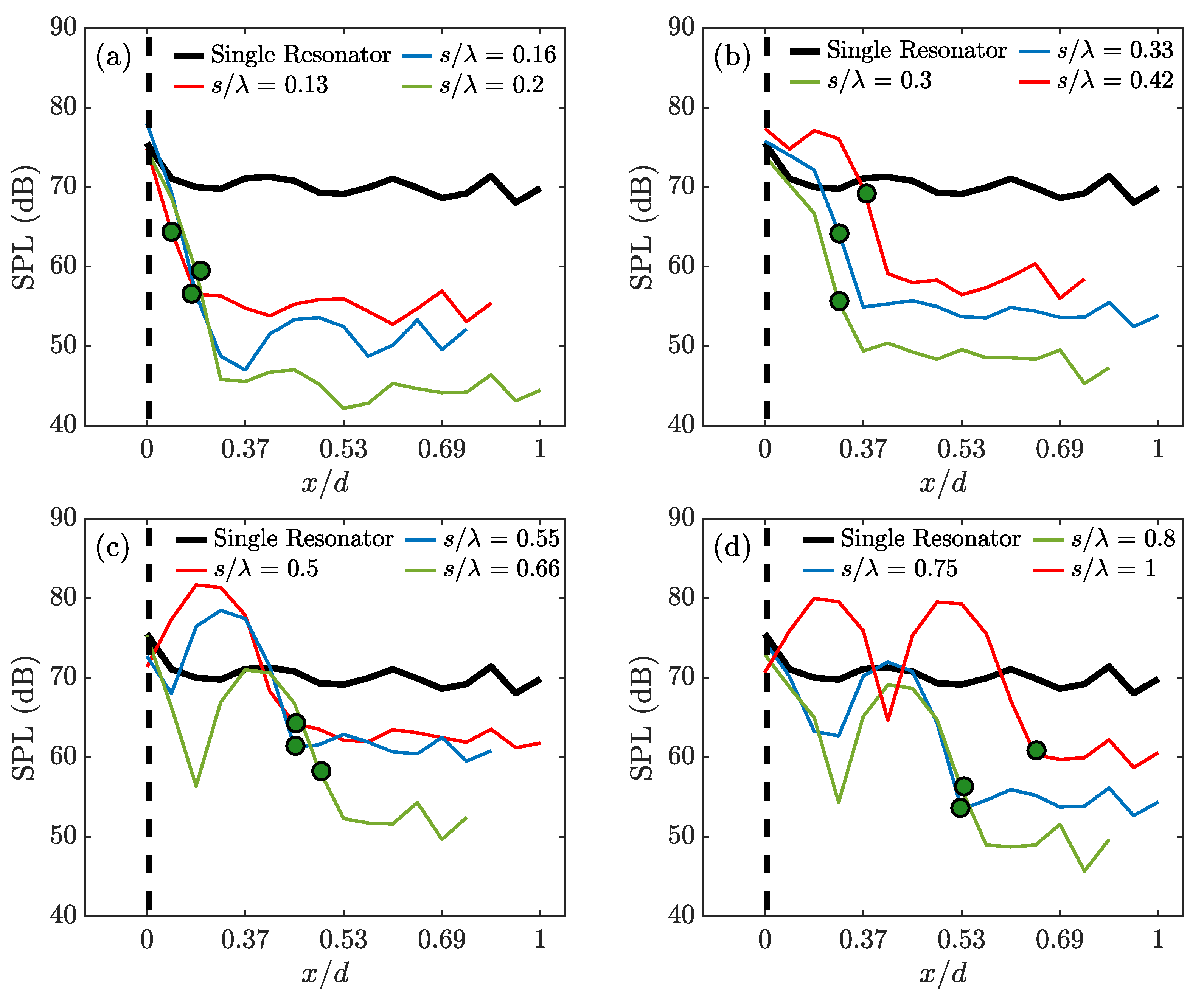
In order to corroborate the sound attenuation patterns observed in Figure 6, data from microphones G1 to G20 were utilised to study the change in the SPL values at the resonance frequency ($f_o=$ 1360 Hz), as the acoustic wave propagates downstream in the impedance tube test section. Figure 7 presents the SPL values against the spacing between the microphones G1 to G20, which are distributed along the impedance tube test section (see Figure 1). The cumulative spacing between the microphones, given by “x”, is non-dimensionalised with the separation distance ‘d’, between microphones, G1 and G20. In order to ease the interpretation, the positions of the first and second resonators are shown with a black dotted line and a green circle, respectively. Considering the results for all spacing configurations (Figure 7a–d), the SPL trend is seen to be significantly affected by the change in the spacing between the resonators. The overall change in sound pressure level, i.e., the difference between SPL values of the microphones G1 and G20, has an oscillating behaviour, which is consistent with the observations presented in Figure 6, and not shown here for brevity. The change in sound pressure level gradually increases with distance between the resonators and reaches a maximum at $s/\lambda =0.2$ (Figure 7a). As shown in Figure 7b,c, as the spacing is further increased, the change in the SPL reduces gradually to a minimum at $s/\lambda =0.5$ (Figure 7c). This trend repeats itself for the separation distances of $s/\lambda =0.75$ (Figure 7d) and $s/\lambda =1$ (Figure 7d), where the SPL change experiences a minimum and maximum, respectively. The cyclic trend seen in the SPL can be attributed to the halfwave resonances in the space between the two resonators. These halfwave resonances can be seen in Figure 6c,d for $s/\lambda =0.5$ and $s/\lambda =1$. The transmission loss induced by a two-resonator system is also limited by this halfwave resonance behaviour that takes place when the distance between the resonators equals to the integer number of half wavelengths.

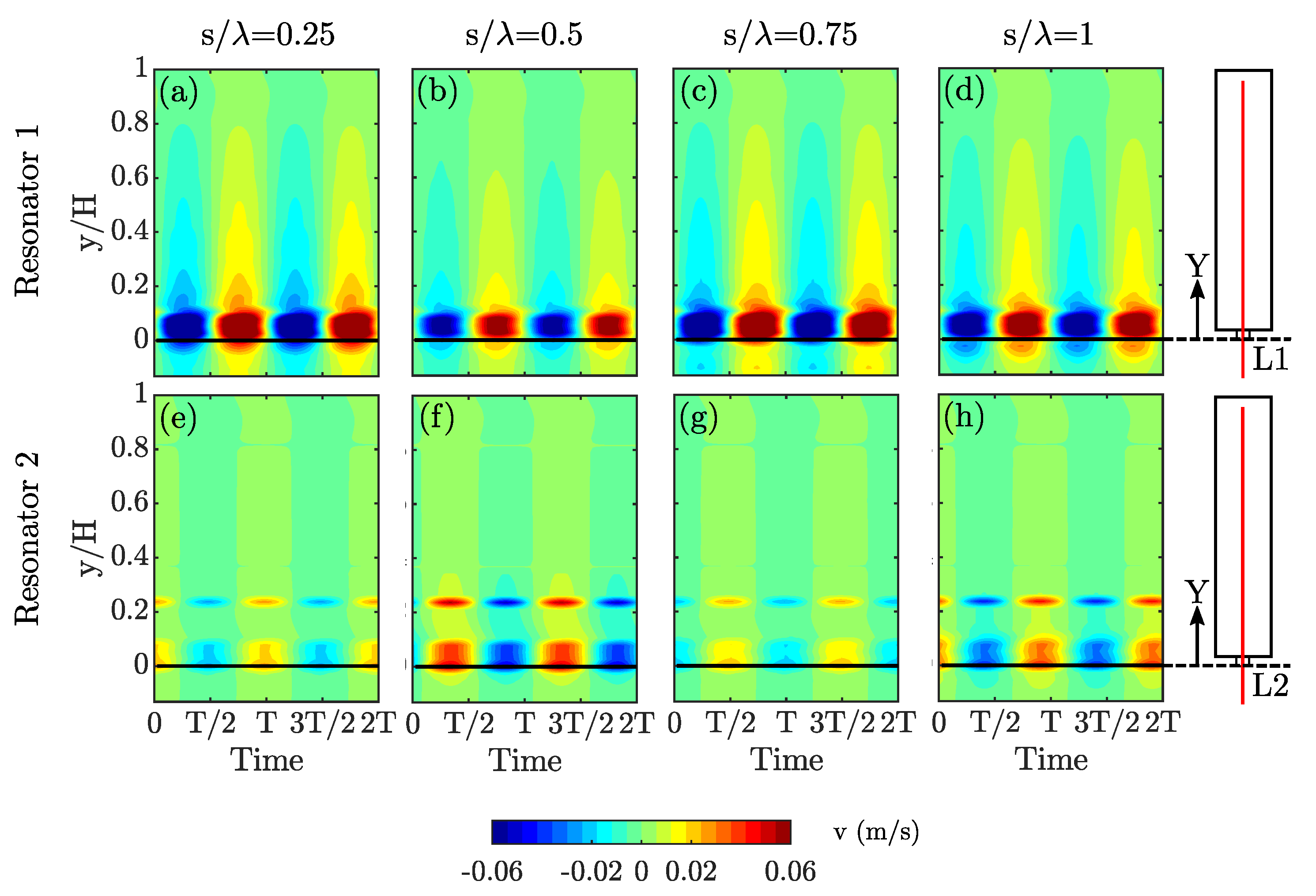
To further explore the underlying physical mechanisms of the sound attenuation behaviour observed in Figure 6 and Figure 7, the acoustic field in the resonator cavities and the impedance tube was investigated in detail by both experimental and numerical studies. To analyse the time dependant nature of both the pressure and velocity fields inside the resonators, transient FEM simulations were carried out using COMSOL Multiphysics${}^{TM}$ at the resonance frequency $f_o$. Due to distinct behaviours observed at $s/\lambda =0.25,0.5,0.75$ and $s/\lambda =1$, the following discussions are shaped around these four spacing configurations. Figure 8 presents the resonator internal pressures, and Figure 9 illustrates the resonator internal particle velocities. Results were obtained using 50 domain probes distributed along the length of the resonators, and denoted by the lines L1 and L2 in associated figures. The domain probes were spaced 1mm apart.

Figure 8a,e show the contour plots of the acoustic pressure inside the two resonators at the resonance frequency over one period (T), for a separation distance of $s/\lambda =0.25$. The figure couples, Figure 8b–d,f–h follow the same structure for $s/\lambda =0.25,0.5,0.75$ and $s/\lambda =1$, respectively. The results indicate that the distance between the resonators affects the relative phase and the cavity internal pressure of the resonators. Considering the results for $s/\lambda =0.25$, Figure 8a,e, it is evident that the pressure magnitudes are significantly lower in Resonator 2 compared to Resonator 1. Moreover, the pressure contours also indicate that both resonators are resonating in phase, as both resonators experience a high and low pressure cycles at a similar time. However, the results at $s/\lambda =0.5$ show a significantly different behaviour compared to the results at $s/\lambda =0.25$. The pressure results indicate an out-of-phase relation between the two resonators, as both resonators experience high and low pressure cycles with a time delay of around T/2. In addition, the pressure levels in Resonator 2 is lower than that of Resonator 1, similar to the results at $s/\lambda =0.25$. Nevertheless, a closer look at the pressure levels for these two spacing configurations, $s/\lambda =0.25$ and $s/\lambda =0.5$, suggests that Resonator 1 experiences an elevated pressure value at $s/\lambda =0.25$ compared to the results of Resonator 1 at $s/\lambda =0.5$. These values are also higher than the values experienced by a single resonator at the resonance frequency, which is not shown here for brevity. Moreover, the pressure values at $s/\lambda =0.25$ for Resonator 2, are significantly lower compared to the results of Resonator 2 at $s/\lambda =0.5$. These results indicate that the pressure magnitude difference between the two resonators reaches its maximum at $s/\lambda =0.25$, while it experiences the minimum difference at at $s/\lambda =0.5$. A similar pattern in terms of pressure magnitude is repeated for $s/\lambda =0.75$ and $s/\lambda =1$, as of $s/\lambda =0.25$ and $s/\lambda =0.5$, respectively. However, the phase relation does not follow this cyclic pattern. As shown in Figure 8c,d,g,h, the two resonators are out-of-phase at $s/\lambda =0.75$ (unlike $s/\lambda =0.25$) and in-phase at $s/\lambda =1$ (unlike $s/\lambda =0.25$).

Taking all of the foregoing observations together, the following outcomes may be underlined. Even though the resonator configurations at $s/\lambda =0.25$ and $s/\lambda =0.75$ result in the highest transmission loss (see Figure 5), the phase relation between the resonators for both cases are not following the same trend. However, for both configurations, the pressure values inside Resonator 1 is significantly elevated, and Resonator 2 is significantly lowered compared to the results of a single resonator. For spacing configurations leading to the broadest bandwidth of attenuated frequencies, i.e., $s/\lambda =0.5$ and $s/\lambda =1$ (Figure 8c,d,g,h), the pressure magnitudes within Resonator 2 is significantly higher than its counterparts at $s/\lambda =0.25$ and $s/\lambda =0.75$, yet still lower than the values of Resonator 1. These results may suggest that a high transmission loss is induced when the performance of Resonator 1 is enhanced by the presence of another resonator, whereas a wide bandwidth of frequencies is attenuated when both resonators exhibit similar cavity pressure magnitudes.

To further elucidate the results presented in Figure 8, the associated particle velocity fields were also assessed and presented. Figure 9 is constructed and presented with the same order as Figure 9 for velocity magnitude contour plots. Figure 9a,b show the contour plots of the internal particle velocity over the associated time period (T) at $s/\lambda =0.25$ for Resonators 1 and 2, respectively. As expected, highest particle velocity magnitude is observed at the neck of the resonators, regardless of the spacing configuration. Moreover, the magnitude of the velocity remains almost constant over all the spacing configurations for Resonator 1. Results of Resonator 2, however, exhibit a different behaviour, and show significantly higher velocity values at $s/\lambda =0.5$ (Figure 9f) and $s/\lambda =1$ (Figure 9h) compared to the results of other spacing values. Interestingly, a second velocity peak is evident inside Resonator 2. Although this second velocity peak is evident for all spacing configurations, it is most prominent for the resonators spacing configurations of $s/\lambda =0.5$ and $s/\lambda =1$. The particle velocity results shown in Figure 9 indicate that the introduction of a second resonator enforces the downstream resonator to deviate from an ideal performance, which may lead to broader bandwidth of attenuated frequencies for spacing configurations of $s/\lambda =0.5$ and $s/\lambda =1$.

3.2. Resonator Acoustic Field Analysis

To further comprehend the observations made with regards to pressure and particle velocity magnitudes in resonator cavities in Figure 8 and Figure 9, the frequency–energy content of the acoustic pressure field inside the resonators was assessed using the experimental data. The sound pressure levels (SPL) were calculated for the data obtained from the flush-mounted surface microphones M1 and M2 (see Figure 1 and Figure 2). Since the speaker was excited with a white noise signal, the effect of the spacing on the performance of the two resonators can be observed over a broad range of frequencies.

Figure 10 presents the comparison of SPL results obtained for data from microphone M1 (Resonator 1) and M2 (Resonator 2) at four different resonator spacing configurations, i.e., $s/\lambda =0.25$, $s/\lambda =0.5$, $s/\lambda =0.75$ and $s/\lambda =1$. Figure 10a provides a comparison of the SPL spectra calculated for the pressure data obtained from microphones M1 and M2 at a spacing of $s/\lambda =0.25$ over a frequency range of 1000 Hz $<f<$ 2000 Hz. The SPL spectra for the other three spacing configurations, $s/\lambda =0.5$, $s/\lambda =0.75$, and $s/\lambda =1$, are presented in Figure 10b–d, respectively. The SPL values obtained for Resonator 1 (M1) indicate that the energy content is highest at around the design frequency of the resonators, i.e., $f_o=1360$ Hz. However, the SPL pattern in Resonator 2 suggests a completely different behaviour. The single peak behavior observed in the first resonator is changed into a double peaked behavior, where the energy content at $f_o$ and surrounding frequencies are vastly subdued. This anti-resonance-like behavior only affects a narrow frequency range around 1280 Hz $<f<1420$ Hz, whereas the rest of the SPL trend is similar to that of M1, with a slight increase in the magnitude for the rest of the domain. These results may be attributed to the high transmission loss characteristics observed for $s/\lambda =0.25$ and $s/\lambda =0.75$, and broad range of effected frequencies for $s/\lambda =0.5$ and $s/\lambda =1$.

To elucidate the peculiar nature observed for the downstream resonator, the coherence between the signals from microphones M1 and M2 was analysed for four different spacing configurations of $s/\lambda =0.25$, $s/\lambda =0.5$, $s/\lambda =0.75$, and $s/\lambda =1$, and is presented in Figure 11. The magnitude-squared coherence is defined as,

$${\gamma }_{M1,M2}^2\left(f\right)=\frac{{\left|P_{M1M2}\left(f\right)\right|}^2}{\left|P_{M1M1}\left(f\right)\right|\left|P_{M2M2}\left(f\right)\right|},$$

(19)

where $P_{M1M1}$ and $P_{M2M2}$ are the power spectral densities of the pressure fluctuations obtained from microphones located at a distance, and $P_{M1M2}$ is the cross-power spectral density of the pressure fluctuations between microphones. The y-axis of the Figure 11 represents the magnitude-squared coherence estimate, which illustrates the level of similarity between the signals from microphone M1 to that from microphone M2 at each frequency. The results show that the pressure signals collected by microphones M1 and M2, inside Resonator 1 and 2, respectively, are strongly coherent around the resonance frequency ($f_o=1360$ Hz) for $s/\lambda =0.5$ and $s/\lambda =1$, which also represent the cases for high transmission loss. However, the coherence trend for the two resonators is considerably different for $s/\lambda =0.25$ and $s/\lambda =0.75$, where Resonator 1 and 2 are, respectively, only 72% and 57% coherent at their design resonance frequency. This observation further corroborates that in a system of two Helmholtz resonators, the resonance frequency of downstream resonator significantly affected by the distance. Although characterising the acoustic field inside the resonator can offer considerable insight into its sound attenuation mechanism, the resonators’ effect on the acoustic field in the duct has to be investigated to form a complete impression.

3.3. Impedance Tube Acoustic Field Analysis

The previously discussed (in Section 3.2) effects of introducing a second resonator on the energy-frequency content of each resonator’s pressure field may also be observed in the acoustic pressure field in the impedance tube. These effects may also shed light on the transmission loss and transmission coefficient behaviour observed in Figure 6. To observe this effect, the coherence between microphones M1, M2, and microphones G3 to G18, flush mounted to the sidewall of the impedance tube, was analysed and presented in Figure 12. A frequency band between 1000 Hz $<f<2000$ Hz is presented to highlight the region of interest around $f_o$. Figure 12a shows the contour plot of magnitude-squared coherence calculated between microphone M1 of a single resonator, i.e., in the absence of the second resonator, and all microphones along the impedance tube, G1 to G20 (see Figure 1). The location of every microphone (x) is normalised by the distance between microphones G1 and G20. Similarly, Figure 12b,c provide the contour plots of magnitude-squared-coherence for the two resonator configuration with a resonator spacing of $s/\lambda =0.25$. The magnitude-squared-coherence was calculated between M1 and microphones located in the impedance tube, G1 to G20 (Figure 12b) and between M2 and microphones G1 to G20 (Figure 12c), respectively. Figure 12d,e present the magnitude-squared-coherence values with a similar approach for $s/\lambda =0.5$.

The magnitude-squared-coherence values obtained between the pressure signals from M1 and the microphones in the tube, G1 to G20, are significantly high around frequencies of 1320 Hz $<f<1420$ Hz along the whole duct length, as shown in Figure 1. To ease the interpretation of the results, the bandwidth of the frequencies with significantly high coherence values (${\gamma }_{p_i{p}_j}^2>$ 0.9), which envelops the resonance frequency of the resonator, is defined as $\Delta F_{HC}$. Figure 12b–e present the contour plots of the magnitude-squared-coherence values for the two-resonator configuration with a spacing of $s/\lambda =0.25$ (Figure 12b,c), and $s/\lambda =0.5$ (Figure 12d,e), respectively. A comparison of the $\Delta F_{HC}$ for $s/\lambda =0.25$ against to that of a single resonator shows a similar bandwidth of the high coherence region for Resonator 1 (shown in Figure 12b). This indicates that for $s/\lambda =0.25$, the first resonator behaves similarly to a single resonator mounted onto the impedance tube, with a complete loss of coherence at a narrow region around the resonance frequency ($f_o$), starting from $x/d=0.5$ and onwards (highlighted with a dashed rectangle). Considering the results for Resonator 2, $\Delta F_{HC}$ increases significantly compared to Resonator 1. However, the increase of $\Delta F_{HC}$ is accompanied by a complete loss of coherence at the resonance frequency for all $x/d$ locations. Moreover, the magnitude-squared-coherence values indicate that the second resonator affects a broader band of frequencies within the impedance tube duct compared to the first resonator, which reaffirms the previous observations discussed for SPL values in Figure 10. For results at $s/\lambda =0.5$ (Figure 12c,d), the coherence values show a significant increase compared to the single resonator case for both resonators. In addition, the results for both resonators exhibit a very similar contour map and a broadened $\Delta F_{HC}$ magnitude. This indicates that both resonators together affect a broad band of frequencies in the duct, unlike the results at $s/\lambda =0.25$.

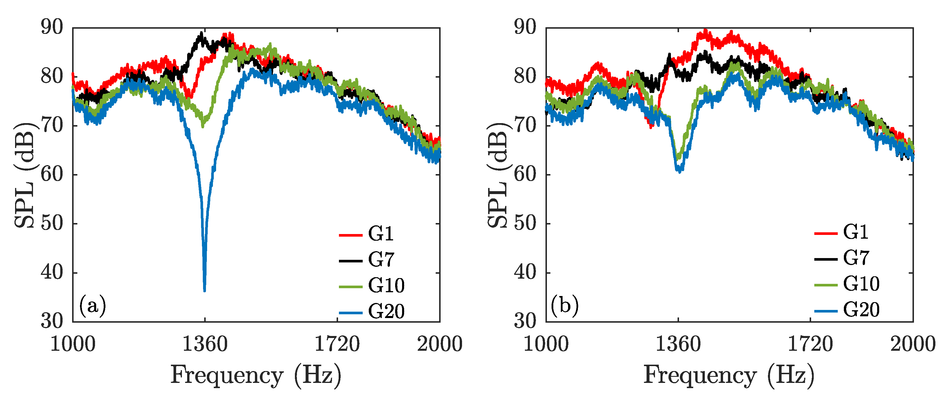
The effect of introducing a second resonator and its distance to the upstream resonator can also be studied through the change in the pressure energy content along the impedance tube. Figure 13 presents the SPL spectra calculated from the signals acquired by microphones G1 to G20 along the impedance tube. For brevity and clarity of the figures, only results at G1, G7, G10, and G20 are presented. Figure 13a shows the SPL spectra of the farthest upstream (G1) and downstream (G20) microphones and the two microphones directly opposite the resonator openings(G7 and G10), at a separation distance of $s/\lambda =0.25$. The results show that the SPL values begin to decrease after the second resonator at around the design frequency. Moreover, the SPL decreases gradually until the last microphone. This indicates that for $s/\lambda =0.25$, the transmission loss introduced by the resonator couple increases as the wave propagates downstream. On the contrary, the results for $s/\lambda =0.5$ show a significantly different behaviour. The results show that the SPL values remain constant after the second resonator and exhibit a lower level of reduction compared to results at $s/\lambda =0.25$.

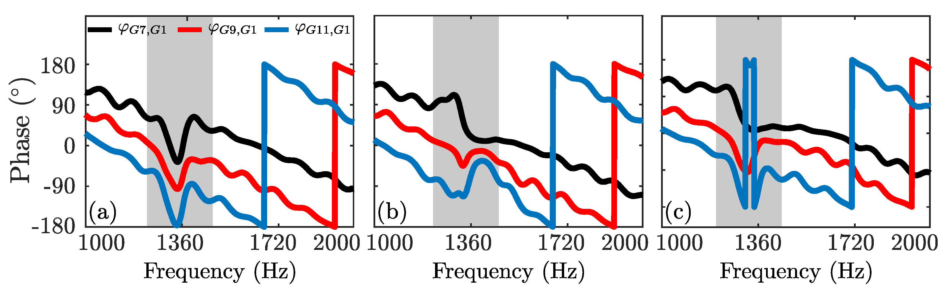
The relative phase information ($\phi$) along the impedance tube may also provide insight into the effect of distance on the noise attenuation performance of the two resonator system. The relative phase was calculated based on the cross-spectral calculations between the downstream microphones (G7, G9, and G11) and the upstream microphone, G1. Figure 14 presents the relative phase information for a single resonator (Figure 14a) and a two-resonator system with $s/\lambda =0.25$ (Figure 14b), and $s/\lambda =0.5$ (Figure 14c). The results are presented for the frequency range, 1000 Hz $<f<2000$ Hz. In Figure 14a, where the results for a single resonator are presented, the relative phase shows a significant change around the resonance frequency. This region is highlighted with a rectangle in the figure to ease the interpretation. The steep decrease in the relative phase indicates a reduction in the speed of propagation around the resonance frequency, which can be observed from the results of all microphones presented [34]. The introduction of a second resonator at $s/\lambda =0.25$ completely alters the relative phase around the resonance frequency. The observed steep decrease in phase for the single resonator yield to a steep increase at the first resonator location (G7) and downstream location in the tube (G11). Interestingly, the relative phase at the location of the second resonator (G9) has a slight increase compared to other microphones. This narrow band increase in phase for all microphones indicates an increase in the propagation speed. At $s/\lambda =0.5$, the relative phase exhibits a trend which is similar to that of the single resonator. However, it is worth mentioning that the dip observed at the resonance frequency for a single resonator is less apparent in this case, and is more of a steep decrease at G7 without recovering to its original path. This indicates a change, in this case an increase, in the propagation speed for the frequencies beyond the resonance frequency.

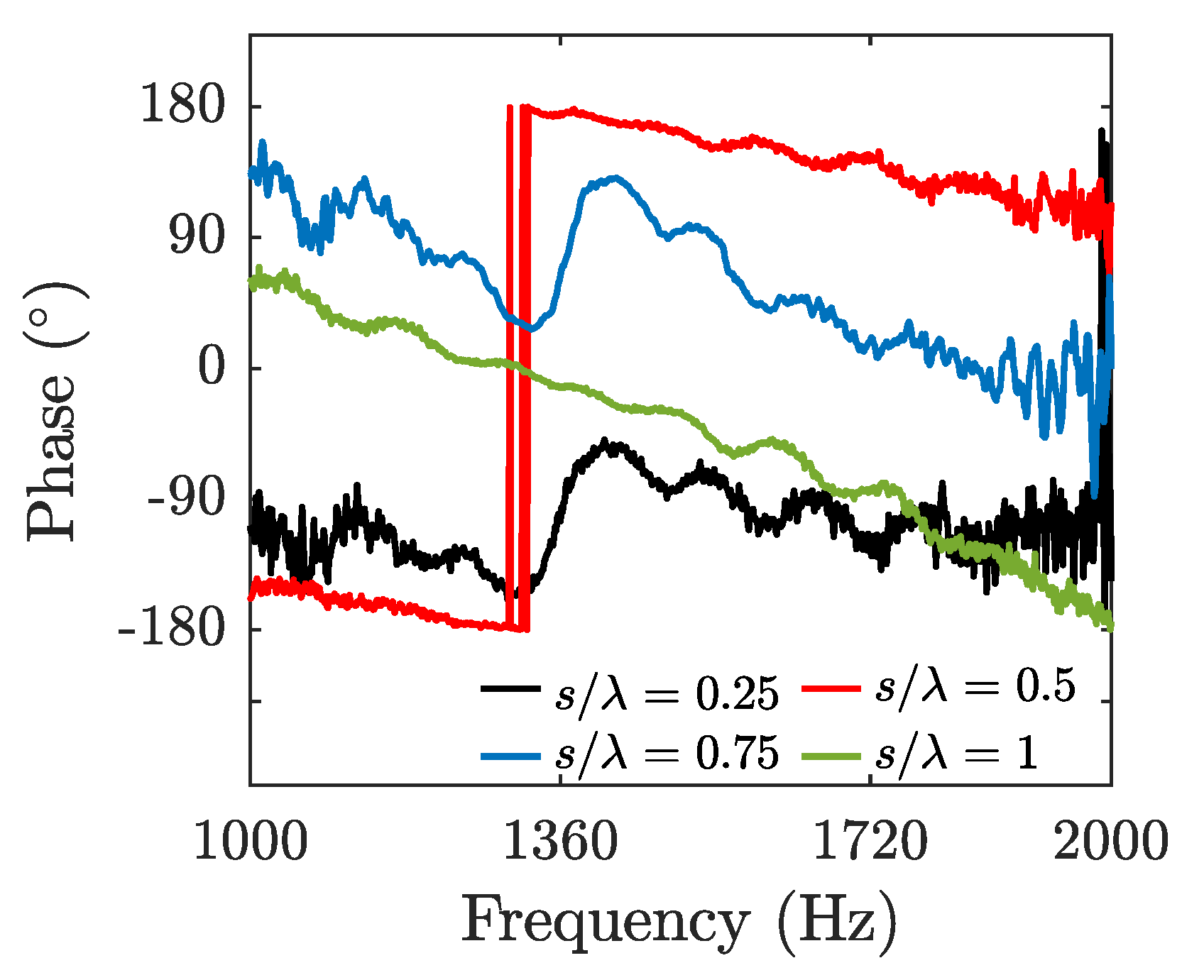
The relative phase between the microphones located in the resonators (M1 and M2) may also shed some light on the effects of resonators spacing on sound attenuation performance of the system. Figure 15 presents the relative phase of the signals obtained from M2 to M1 (${\phi }_{M2,M1}$) at four different spacing configurations, $s/\lambda =0.25,0.5,0.75$ and $s/\lambda =1$. The results show that at $s/\lambda =0.25$ and $s/\lambda =0.75$, where the highest transmission loss occur, the relative phase increases at around the resonance frequency and indicates an increase in the propagation speed. On the contrary, at $s/\lambda =0.5$ and $s/\lambda =1$, the relative phase shows a gradual decrease, which implies that the phase relation between the resonators does not alter around the resonance frequency. These observations are consistent with the previous results shown in Figure 14.

4. Conclusions

The effect of the spacing between two Helmholtz resonators mounted in an impedance tube is studied to explore its effect on the transmission loss and sound pressure level change. The investigation is conducted both experimentally and numerically. The experiments were performed in a grazing impedance tube with two instrumented resonators. The experimental results showed that the presence of a second resonator can have profound effect on the acoustic performance of the resonator system, which depends on the location of the second resonator relative to the upstream resonator. The sound pressure values measured along the impedance tube showed that decreasing the spacing between the two resonators leads to a higher rate of reduction in the SPL along the tube. Moreover, the results also exhibit that the maximum transmission loss is achieved at separation distances of $s/\lambda =0.25$ and $s/\lambda =0.75$, whereas the broadest frequency band of reduced noise was obtained at separation distances of $s/\lambda =0.5$ and $s/\lambda =1$. The bandwidth coefficient study illustrated that the spacing, transmission loss, and transmission coefficient are related in a way that the spacing configurations that lead to the lowest transmission loss value result in the widest range of frequencies being attenuated and vice-versa. The numerical studies revealed a complex relation of pressure, particle velocity and the relative phase between the resonators. The results suggest an enhanced pressure value inside the upstream resonator in the presence of a second resonator at distances $s/\lambda =0.25$ and $s/\lambda =0.75$. However, at this spacing configurations, the downstream resonator experiences the lowest pressure levels compared to the results of other configurations. Moreover, at spacing configurations of $s/\lambda =0.5$ and $s/\lambda =1$, the pressure values inside both resonators are similar. In addition, the particle velocity results inside the Resonator 2 exhibit an unexpected behaviour with two velocity peaks for all spacing configurations with higher magnitudes of particle velocity at $s/\lambda =0.5$ and $s/\lambda =0.1$, where a lower transmission loss is achieved with the broadest bandwidth of frequency. The energy content of the pressure inside downstream resonator exhibits a subdued region at the resonance frequency for the configurations with $s/\lambda =0.25$ and $s/\lambda =0.75$, which might be the reason of observed behaviour in these configurations. The relative phase results show that the separation distance has a pronounced effect not only on the phase relation between the pressure field inside the resonator and the impedance tube but also on the phase relation between the two resonators. The results of this investigation suggest that liners based on Helmholtz resonators can be tailored for different purposes, and by careful positioning of resonators an optimised arrangement can be achieved to maximise the sound pressure level reduction. Moreover, the findings presented in this study can lead to liner designs with enhanced acoustic performance.

References

- Khardi, S. An experimental analysis of frequency emission and noise diagnosis of commercial aircraft on approach. J. Acoust. Emiss. 2008, 26, 290–310. [Google Scholar]
- ACARE. Flightpath 2050-Europe’s Vision for Aviation; Publications Office of the European Union: Luxembourg, 2011. [Google Scholar]
- Spakovszky, Z. Advanced low-noise aircraft configurations and their assessment: Past, present, and future. CEAS Aeronaut. J. 2019, 10, 137–157. [Google Scholar] [CrossRef]
- Dowling, A.; Hynes, T. Towards a silent aircraft. Aeronaut. J. 2006, 110, 487–494. [Google Scholar] [CrossRef]
- Thomas, R.H.; Burley, C.L.; Olson, E.D. Hybrid wing body aircraft system noise assessment with propulsion airframe aeroacoustic experiments. Int. J. Aeroacoustics 2012, 11, 369–409. [Google Scholar] [CrossRef] [Green Version]
- Dannemann, M.; Kucher, M.; Kunze, E.; Modler, N.; Knobloch, K.; Enghardt, L.; Sarradj, E.; Höschler, K. Experimental Study of Advanced Helmholtz Resonator Liners with Increased Acoustic Performance by Utilising Material Damping Effects. Appl. Sci. 2018, 8, 1923. [Google Scholar] [CrossRef] [Green Version]
- Cai, C.; Mak, C.M. Acoustic performance of different Helmholtz resonator array configurations. Appl. Acoust. 2018, 130, 204–209. [Google Scholar] [CrossRef]
- Yang, D.; Wang, X.; Zhu, M. The impact of the neck material on the sound absorption performance of Helmholtz resonators. J. Sound Vib. 2014, 333, 6843–6857. [Google Scholar] [CrossRef]
- Shi, X.; Mak, C.M. Helmholtz resonator with a spiral neck. Appl. Acoust. 2015, 99, 68–71. [Google Scholar] [CrossRef]
- Langfeldt, F.; Hoppen, H.; Gleine, W. Broadband low-frequency sound transmission loss improvement of double walls with Helmholtz resonators. J. Sound Vib. 2020, 476, 115309. [Google Scholar] [CrossRef]
- Park, S.H. Acoustic properties of micro-perforated panel absorbers backed by Helmholtz resonators for the improvement of low-frequency sound absorption. J. Sound Vib. 2013, 332, 4895–4911. [Google Scholar] [CrossRef]
- Tang, S.K. On Helmholtz resonators with tapered necks. J. Sound Vib. 2005, 279, 1085–1096. [Google Scholar] [CrossRef]
- Komkin, A.I.; Mironov, M.A.; Bykov, A.I. Sound absorption by a Helmholtz resonator. Acoust. Phys. 2017, 63, 385–392. [Google Scholar] [CrossRef]
- Rayleigh, J.W.S.B. The Theory of Sound; Macmillan: New York, NY, USA, 1896; Volume 32. [Google Scholar]
- Ingard, U. On the theory and design of acoustic resonators. J. Acoust. Soc. Am. 1953, 25, 1037–1061. [Google Scholar] [CrossRef]
- Chanaud, R. Effects of geometry on the resonance frequency of Helmholtz resonators. J. Sound Vib. 1994, 178, 337–348. [Google Scholar] [CrossRef]
- Dickey, N.; Selamet, A. Helmholtz resonators: One-dimensional limit for small cavity length-to-diameter ratios. J. Sound Vib. 1996, 195, 512–517. [Google Scholar] [CrossRef]
- Selamet, A.; Radavich, P.; Dickey, N.; Novak, J. Circular concentric Helmholtz resonators. J. Acoust. Soc. Am. 1997, 101, 41–51. [Google Scholar] [CrossRef]
- Selamet, A.; Ji, Z. Circular asymmetric Helmholtz resonators. J. Acoust. Soc. Am. 2000, 107, 2360–2369. [Google Scholar] [CrossRef]
- Selamet, A.; Lee, I. Helmholtz resonator with extended neck. J. Acoust. Soc. Am. 2003, 113, 1975–1985. [Google Scholar] [CrossRef]
- Cai, C.; Mak, C.M.; Shi, X. An extended neck versus a spiral neck of the Helmholtz resonator. Appl. Acoust. 2017, 115, 74–80. [Google Scholar] [CrossRef]
- Coulon, J.M.; Atalla, N.; Desrochers, A. Optimization of concentric array resonators for wide band noise reduction. Appl. Acoust. 2016, 113, 109–115. [Google Scholar] [CrossRef]
- Cai, C.; Mak, C.M.; Wang, X. Noise attenuation performance improvement by adding Helmholtz resonators on the periodic ducted Helmholtz resonator system. Appl. Acoust. 2017, 122, 8–15. [Google Scholar] [CrossRef]
- Wu, D.; Zhang, N.; Mak, C.M.; Cai, C. Hybrid noise control using multiple Helmholtz resonator arrays. Appl. Acoust. 2019, 143, 31–37. [Google Scholar] [CrossRef]
- Nagaya, K.; Hano, Y.; Suda, A. Silencer consisting of two-stage Helmholtz resonator with auto-tuning control. J. Acoust. Soc. Am. 2001, 110, 289–295. [Google Scholar] [CrossRef]
- Cheng, C.R.; McIntosh, J.D.; Zuroski, M.T.; Eriksson, L.J. Tunable Acoustic System. U.S. Patent 5,930,371, 27 July 1999. [Google Scholar]
- de Bedout, J.M.; Franchek, M.A.; Bernhard, R.J.; Mongeau, L. Adaptive-passive noise control with self-tuning Helmholtz resonators. J. Sound Vib. 1997, 202, 109–123. [Google Scholar] [CrossRef] [Green Version]
- International, A. E2611-19 Standard Test Method for Normal Incidence Determination of Porous Material Acoustical Properties Based on the Transfer Matrix Method; ASTM International: West Conshohocken, PA, USA, 2019. [Google Scholar] [CrossRef]
- Ali, S.A.S. Flow Over and Past Porous Surfaces. Ph.D. Thesis, University of Bristol, Bristol, UK, 2018. [Google Scholar]
- Langfeldt, F.; Hoppen, H.; Gleine, W. Resonance frequencies and sound absorption of Helmholtz resonators with multiple necks. Appl. Acoust. 2019, 145, 314–319. [Google Scholar] [CrossRef]
- Welch, P. The use of fast Fourier transform for the estimation of power spectra: A method based on time averaging over short, modified periodograms. IEEE Trans. Audio Electroacoust. 1967, 15, 70–73. [Google Scholar] [CrossRef] [Green Version]
- Mechel, F.P. Formulas of Acoustics; Springer: Berlin/Heidelberg, Germany, 2004. [Google Scholar]
- Multiphysics, C. Introduction to Acoustics Module; COMSOL AB: Stockholm, Sweden, 2012. [Google Scholar]
- Olfert, J.S.; Checkel, M.D.; Koch, C.R. Acoustic method for measuring the sound speed of gases over small path lengths. Rev. Sci. Instruments 2007, 78, 054901. [Google Scholar] [CrossRef] [Green Version]
Figure 1.
Schematics of the (a) grazing flow impedance tube, (b) the test section of the impedance tube with microphone naming convention and the cross section-view of the test section.
Figure 2.
Schematics of a resonator sample with geometrical details and locations of the flush-mounted microphone (pressure transducer) inside the Helmholtz resonator.
Figure 3.
Comparison of transmission coefficient for different resonator sealing configurations.
Figure 4.
Schematics of two Helmholtz resonators mounted in line.
Figure 5.
(a) Experimental results for transmission coefficient induced by different spacing () configurations; (b) Experimental results for transmission loss induced by different spacing () configurations.
Figure 6.
(a) Normalised transmission loss comparison for different spacing configurations; (b) Bandwidth Coefficient comparison for different spacing configurations.
Figure 7.
Change in the SPL value at resonance frequency () in the impedance tube for different spacing configurations between . (a) , (b) , (c) , (d) .
Figure 8.
Contour plots of pressure inside the resonators for different spacing configurations between . Top row: Sound pressure field within the first resonator for (a) ; (b) ; (c) ; (d) ; Bottom row: Sound pressure field within the second resonator for (e) ; (f) ; (g) ; (h) .
Figure 9.
Contour plots of particle velocity for different spacing configurations between . Top row: Particle velocity field within the first resonator for (a) ; (b) ; (c) ; (d) ; Bottom row: Particle velocity field within the second resonator for (e) ; (f) ; (g) ; (h) .
Figure 10.
SPL of acoustic signal from microphone M1 and M2 for different spacing configurations between 0.25 < <1. (a) ; (b) ; (c) ; (d) .
Figure 11.
Coherence of acoustic signal from microphone M1 and M2 for different spacing configurations between 0.25 < < 1.
Figure 12.
Magnitude squared coherence of acoustic signal from microphone M1 and M2 with microphones G1 to G20. (a) Single Resonator; (b) (Resonator 1); (c) (Resonator 2); (d) (Resonator 1); (e) (Resonator 2).
Figure 13.
SPL of the acoustic signal from microphones G1 to G20. (a) ; (b) .
Figure 14.
Phase of the pressure signals from microphone G7,G9 and G11 compared with G1 for different resonator configurations. (a) Single Resonator; (b) ; (c) .
Figure 15.
Phase of the pressure signal from M2 relative to M1 for spacing configurations of and .
Publisher’s Note: MDPI stays neutral with regard to jurisdictional claims in published maps and institutional affiliations. |
© 2021 by the authors. Licensee MDPI, Basel, Switzerland. This article is an open access article distributed under the terms and conditions of the Creative Commons Attribution (CC BY) license (http://creativecommons.org/licenses/by/4.0/).
Share and Cite
MDPI and ACS Style
Gautam, A.; Celik, A.; Azarpeyvand, M. An Experimental and Numerical Study on the Effect of Spacing between Two Helmholtz Resonators. Acoustics 2021, 3, 97-117. https://0-doi-org.brum.beds.ac.uk/10.3390/acoustics3010009
AMA Style
Gautam A, Celik A, Azarpeyvand M. An Experimental and Numerical Study on the Effect of Spacing between Two Helmholtz Resonators. Acoustics. 2021; 3(1):97-117. https://0-doi-org.brum.beds.ac.uk/10.3390/acoustics3010009
Chicago/Turabian StyleGautam, Abhishek, Alper Celik, and Mahdi Azarpeyvand. 2021. "An Experimental and Numerical Study on the Effect of Spacing between Two Helmholtz Resonators" Acoustics 3, no. 1: 97-117. https://0-doi-org.brum.beds.ac.uk/10.3390/acoustics3010009