Article

Optimization Model for Fresh Fruit Supply Chains: Case-Study of Dragon Fruit in Vietnam

1
Department of Industrial Engineering, Dalhousie University, PO BOX 15000, Halifax, NS B3H 4R2, Canada
2
Biofluids and Biosystems Modeling Lab. (BBML), Department of Engineering, Faculty of Agriculture, Dalhousie University, 39 Cox Road, Truro, NS B2N 5E3, Canada
3
School for Resource and Environmental Studies, Dalhousie University, 6100 University Ave, PO BOX 15000, Halifax, NS B3H 4R2, Canada
*
Author to whom correspondence should be addressed.
Submission received: 4 November 2019 / Revised: 13 December 2019 / Accepted: 16 December 2019 / Published: 20 December 2019

Abstract

:
We present an optimization model for dragon fruit plantations in Vietnam. The timing of cultivating and harvesting decisions are taken into account as the dragon fruit plant has an approximately ten-year life cycle with maximum average yield in the fourth year. Another consideration also included is the prevalence of forward-buying contracts with locked-in prices. The dragon fruit supply chain faces several difficulties as yield, price, and demand are highly sensitive to weather conditions and global uncertainty factors. The risk factors in the dragon fruit supply chain also depend on species—for example, the red varieties, while more profitable than the white varieties, also have higher export risk because they are subject to global prices and adverse geopolitical conditions.

1. Introduction

In recent years, along with the development of the supply chain management and logistics industry, the agri-food supply chain in general and the fresh fruit chain in particular have been recognized as strategic components of the national economy of many developing countries such as Vietnam.
Compared to staple crops, fruit production brings greater economic benefits. However, the fruit and vegetable production sector also faces particular risks such as climate change, water scarcity, increase in land-use for industrial and urban development, and consumer behavior and price volatility. Moreover, the planning and managing of production, distribution, and pricing of fresh fruits are more complicated because of their very short shelf-life.
The value can be increased if the value chain of fruit and vegetable production and distribution is better organized from farmers to retailers. Countries where agriculture is in development, i.e., Vietnam, are still facing challenges such as:
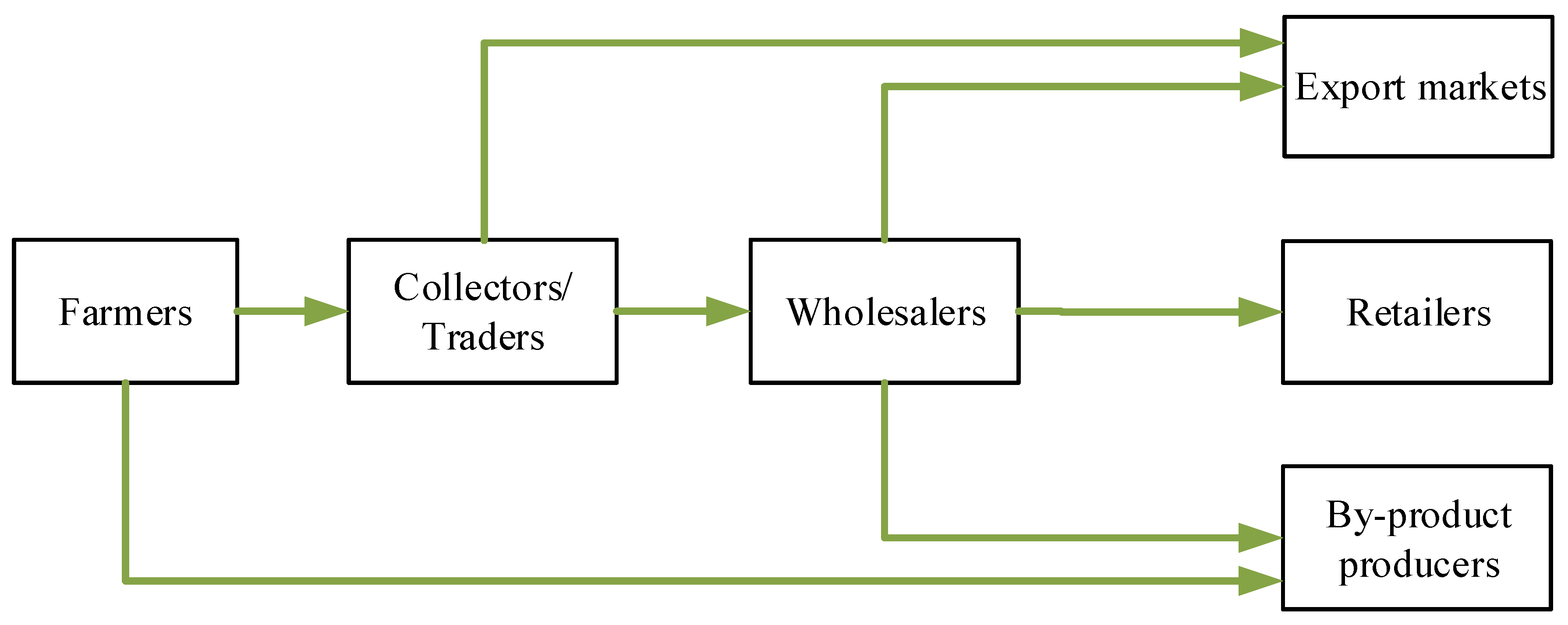
  • The influence of traditional trade practices—there are many intermediate nodes involved in the network, making the food supply chain longer and more complex than in other developed countries.
  • The high cost of storage after harvesting and transportation—this is due to the tropical climate with high temperature and humidity.
  • The continued use of low paid labor. Though labor is cheap, there is a high workforce turnaround. The workforce shortages are acute at the beginning and end of the harvest season when labor demand is high due to competition. During these periods, workers often change employers for better pay.
  • The poor availability of information within the value chain from growers to collectors/traders, wholesalers, retailers, and supermarkets about the harvest, preliminary processing, packing, labeling, preserving, and transportation.
  • The inability of farmers to set produce prices—farmers play the most important role in the food supply chain but most of them are small, with little influence on price. They must sell their products at prices determined by traders due to lack of market information and experience.
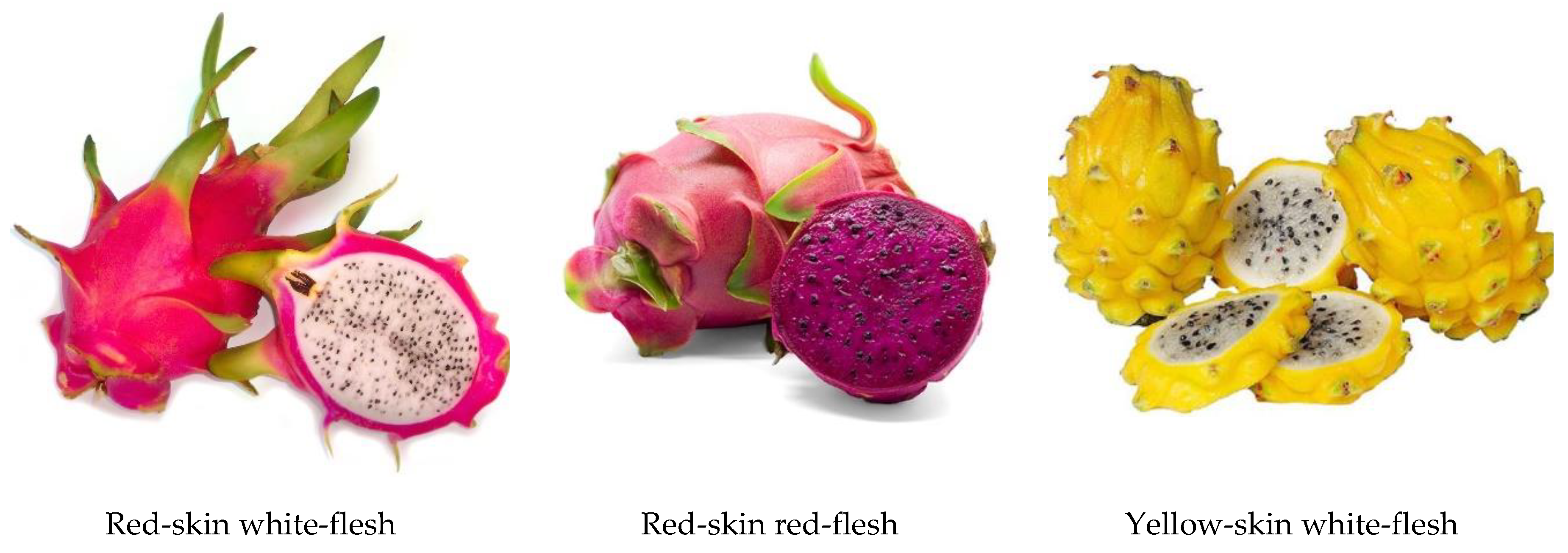
  • Due to the lack of long-term orientation at the macro-level of management, farmers target profits based on market demand. In the dragon fruit case, this may imply cutting existing varieties of the fruit and changing over to other varieties, based on anticipated demand. Since dragon fruit is a perennial plant, the impact of these decisions can last several years.
It can be said that making decisions for a fresh fruit supply chain management is a more difficult and complex problem than with other supply chains [1]. This is a great challenge for fresh fruit supply chain (FFSC) managers over the past 40 years, given the increasing globalization and rapidly increasing demand. They need a tool to support modern and accurate decision-making for long-term production. There are several articles in the literature related to FFSCs with many different approaches or methods that could support optimization of a part or the whole chain. The deterministic approach is a very common and often used in the FFSC research; formulations are based on both linear programming [2,3,4,5,6,7] and mixed integer programming [8,9,10,11,12,13,14,15,16,17].
There are two essential types of fruit used for case studies: perennial crops such as apples [18,19,20,21], oranges [6,12], pome fruit [10], pears [16,22,23], cherries [24] and grapes [4,25,26] or annual crops such as pineapple [27], strawberries [28], melon [29], and tomato [13,30,31]. Dragon fruit is a tropical fast-growing perennial crop, other examples being asparagus [32], Persian lime [33], Thai soursop, Taiwan pear-shaped guava, etc.
During the last several years, the fresh produce cold chain has received attention from researchers around the world to enhance the quality and freshness of fruits and vegetables delivered to customers. The cold chain issues considered by most researchers have to do with controlling the temperature and gas flow in containers [34,35,36], minimizing the energy used to refrigerate containers [37], and optimizing the transport system in the chain [38].
The dragon fruit (Figure 1) is a tropical fruit grown extensively in Vietnam. With 36.5 thousand hectares of cultivated land and 630 thousand tons of total yield, Vietnam is the world’s leading exporter of dragon fruit [39]. However, dragon fruit production and processing are still in a nascent stage of development and face issues around severe price fluctuations due to conditions such as:
  • Product development is still nascent;
  • Market price fluctuations;
  • Chinese imports are subject to price and currency exchange risks;
  • High competition with other exporting countries (such as Thailand, Malaysia, etc.) driving down value despite increased export volumes;
  • Export has been increasing both in volume and value but the increase in value has been declining.
This paper presents an optimization model for dragon fruit crop planning to support farmers make decisions on the allocation of land to crop varieties. The objective of the model is to maximize profit, while satisfying customer demand. Given that dragon fruit is perennial but fast growing, there is an opportunity to change the crop mix based on anticipated future prices. However, there could be a loss in yield depending on the maturity of the crops in a plantation mix. The remainder of this paper is organized as follows: Section 2 introduces dragon fruit plantation and crop planning. Section 3 presents a linear programming optimization model for crop harvesting and replantation decisions. Section 4 presents the results and discussions from example scenarios. Section 5 concludes the paper and outlines areas for further study.

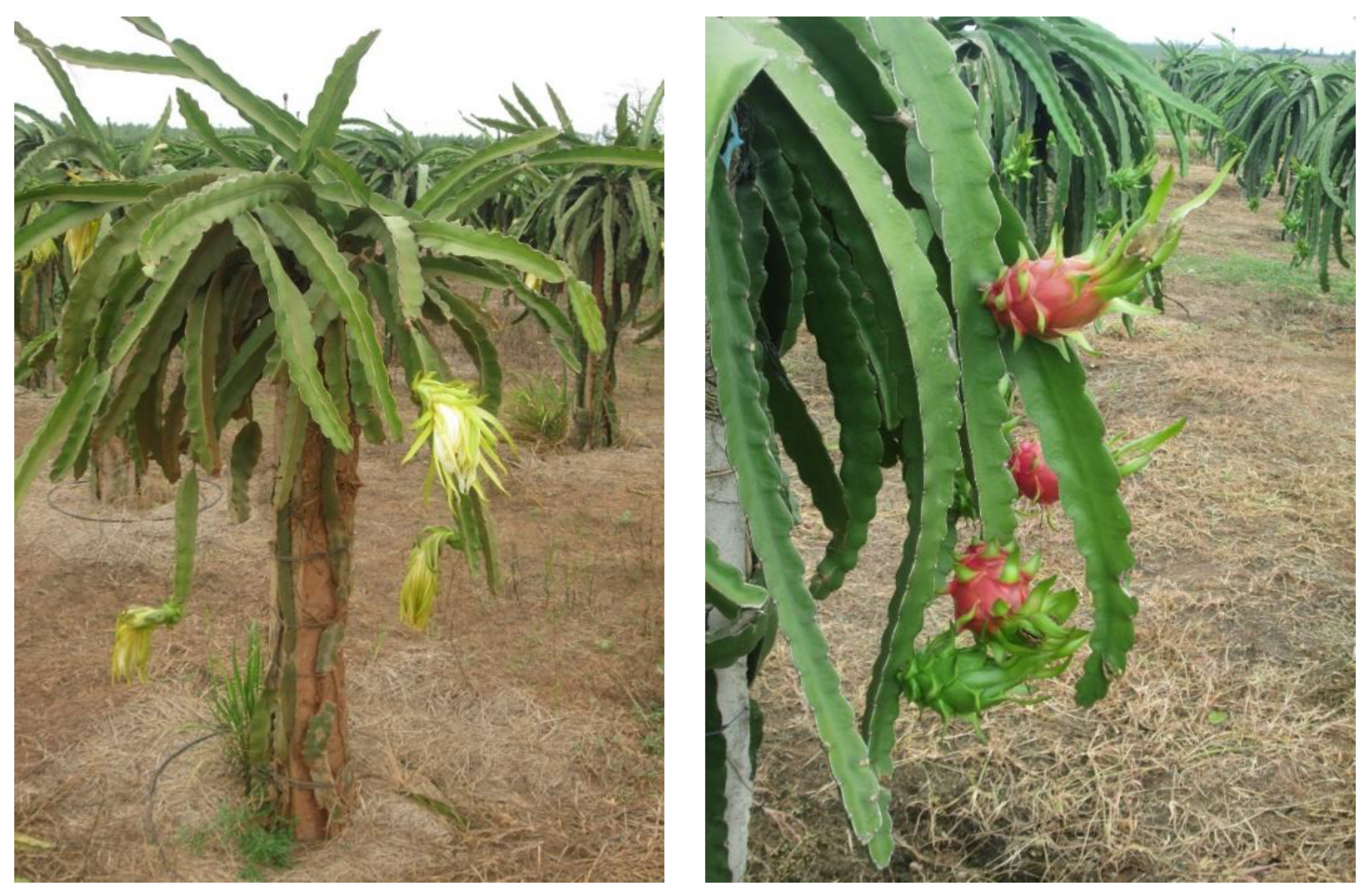
2. Dragon Fruit Plantation Characteristics

2.1. Fruit Distribution Context

The dragon fruit supply chain starts with farmers who make plantation decisions based on forward buy-in contracts with traders. The traders sell fruit to by-products and wholesalers who in turn distribute the fruit and by-products to retail, export, and by-product producers. The dragon fruit supply chain is depicted in Figure 2. Typical dragon fruit by-products are wine and packaged dried fruit snacks.
Dragon fruit is typically planted twice a year in Vietnam. Harvesting starts one year after plantation, but the fruit is at the quality required for commercial purposes 2–10 years after harvest. Dragon fruit yield typically depends on age and a tree is usually only considered productive until the age of 12 years. Figure 3 shows the typical yield curve as a function of tree age (based on [41]).
There are three varieties of dragon fruit planted in Vietnam: the red-skin white-flesh, the red-skin red-flesh and the yellow-skin white-flesh (Figure 4). The red-skin varieties are very popular, the white-flesh variety being the most sold. The red-skin red-flesh variety has a high demand during the lunar New Year and is also exported extensively to China. The yellow peel white flesh variety is relatively new in Vietnam and is available only in major metropolitan areas.
The dragon fruit blooms from May to August and is ready a month later for harvesting in September and October. However, dragon fruit prices are usually low in the main season (due to the availability of the fruit). Due to its high economic value in January and February, dragon fruit growers install lighting systems to stimulate trees to bloom and have fruits to improve productivity in the dry season which lasts from November to April [40]. Therefore, there are two times for harvesting, either from May to October (rainy season or season 1) or from November to April (dry season or season 2) (Figure 5).
Dragon fruit trees are commercially viable for 10–12 years, but because they grow quickly, the plantations can continue to harvest existing crops below that age or cut them down for investment in other varieties based on demand and price.

2.2. Methodology

The methodology in this paper is aligned with the hierarchical planning approach which separates the decision-making process into tactical and operational phases [42]. In hierarchical planning, decisions are first made at the tactical level and then at the operational level. Figure 6, which is adapted from Ahumada et al. [31], shows how the hierarchical approach may be applied to the dragon fruit chain.
In this paper, a quantitative modeling approach for decision making for dragon fruit plantation and harvesting in Vietnam is presented. As previously mentioned, this approach looks at planting and cutting (which are tactical decisions) taken over a multi-year planning horizon. The potential benefit from the hierarchical planning is that growers can be involved in making decisions about the market and production. In other words, coordinating tactical and operational decisions is beneficial for multiple parties: growers, producers, distributors, and vendors.
In Figure 6, the first phase deals with tactical decisions that are only made at the start of the season such as what crop to plant or truncate, and when and how much to plant or truncate. While in the second phase, farmers must decide how much to sell to customers in each season according to the market conditions.
To execute the hierarchical planning schematic, a deterministic optimization model is developed in this paper for the dragon fruit production in Vietnam. Although dragon fruit is used as the main target the current study, our model can certainly be adapted to other fresh fruit production chains.

3. Linear Programming Optimization Model

3.1. Hypotheses and Assumptions

For this model, it is assumed that:
  • The facilities (farms) are already operational since the model does not deal with network decisions.
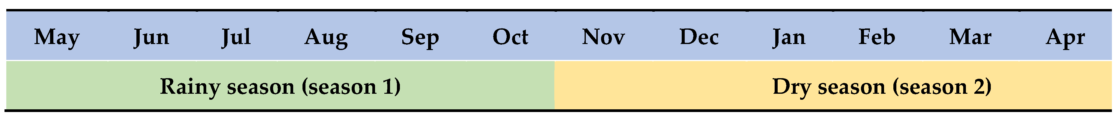
  • The time horizon for tactical planning is 10 years and two harvesting seasons (rainy season and dry season) for each year are considered.
  • Fruit trees are cut down when they are 10 years of age or earlier, if the model chooses to (e.g., when the future prices of other crops are much higher than the planted crop). It is assumed that cutting down or replanting decisions are only carried out in season 1.
  • The distribution of yield, demand, and market prices are represented by their expected values.
  • Storage is not allowed for fresh dragon fruit. However, the fruit may be used for by-products such as dry snacks and wine.
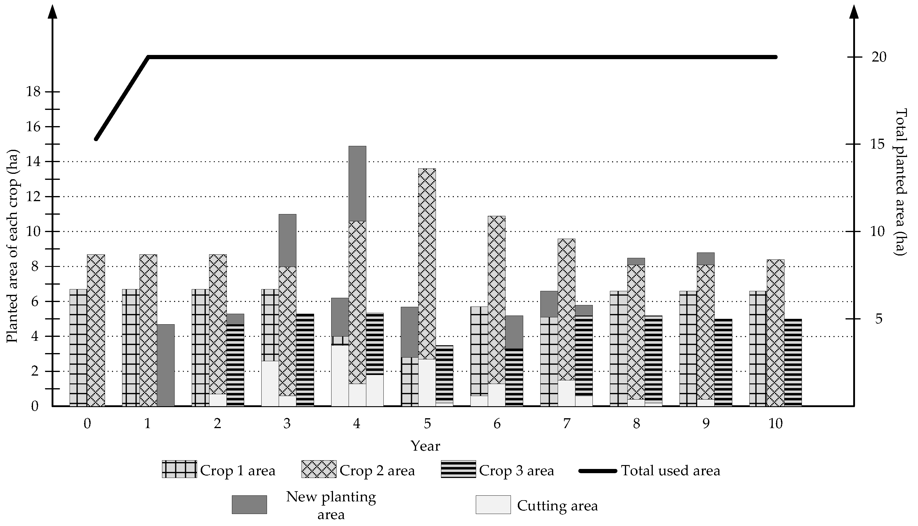
  • The amounts of each crop to cut and plant are decision variables which cannot exceed the maximum amount of land that is already determined.
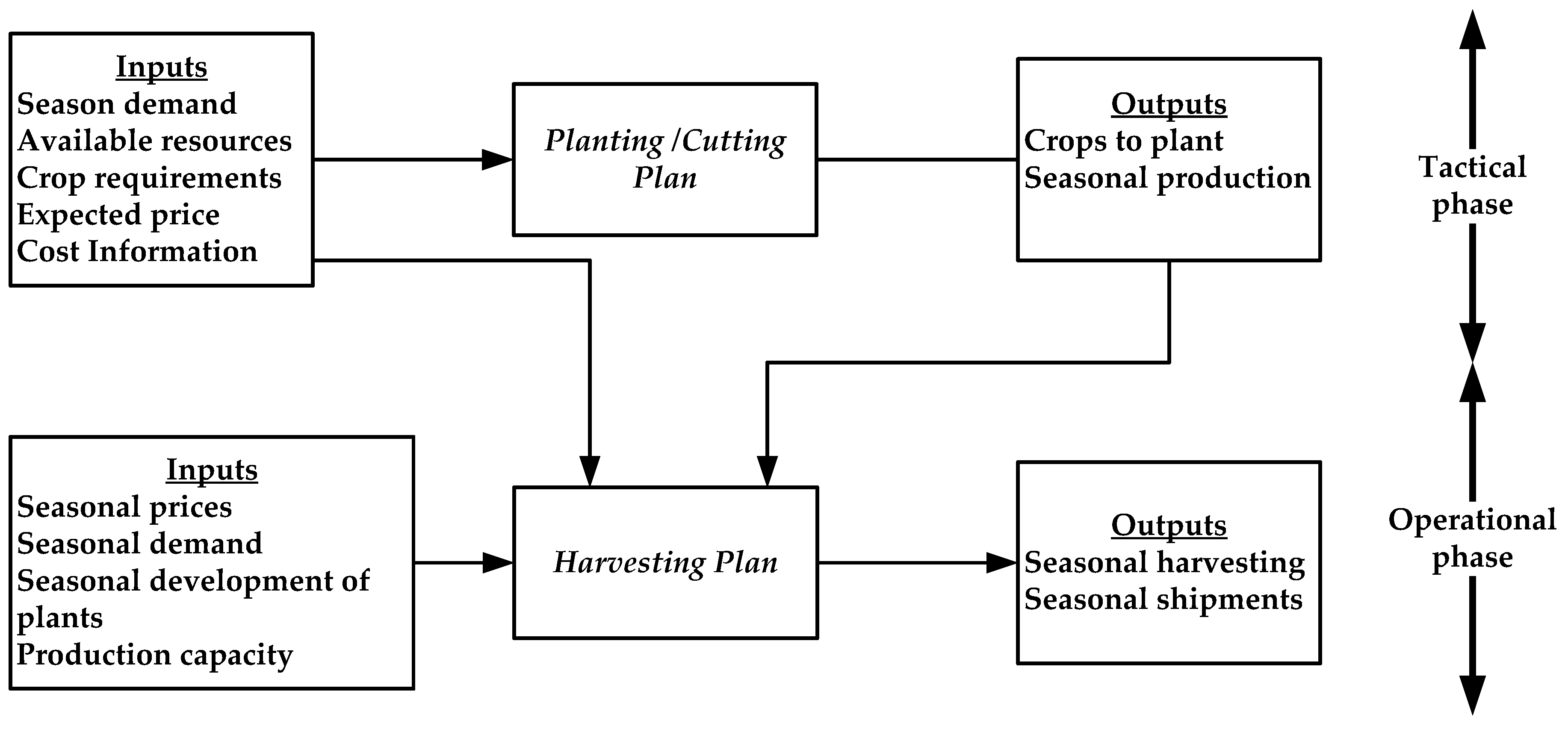
  • Decision variables of the model are the new plantation and truncating areas of each crop, and the amount of fruit sent to customers (traders, wholesalers, and by-product producers) in every year.
  • Other decisions include the quantity of fruit to sell to customers and the amount of labor (fixed and part-time) is required to cover all the activities in the model.

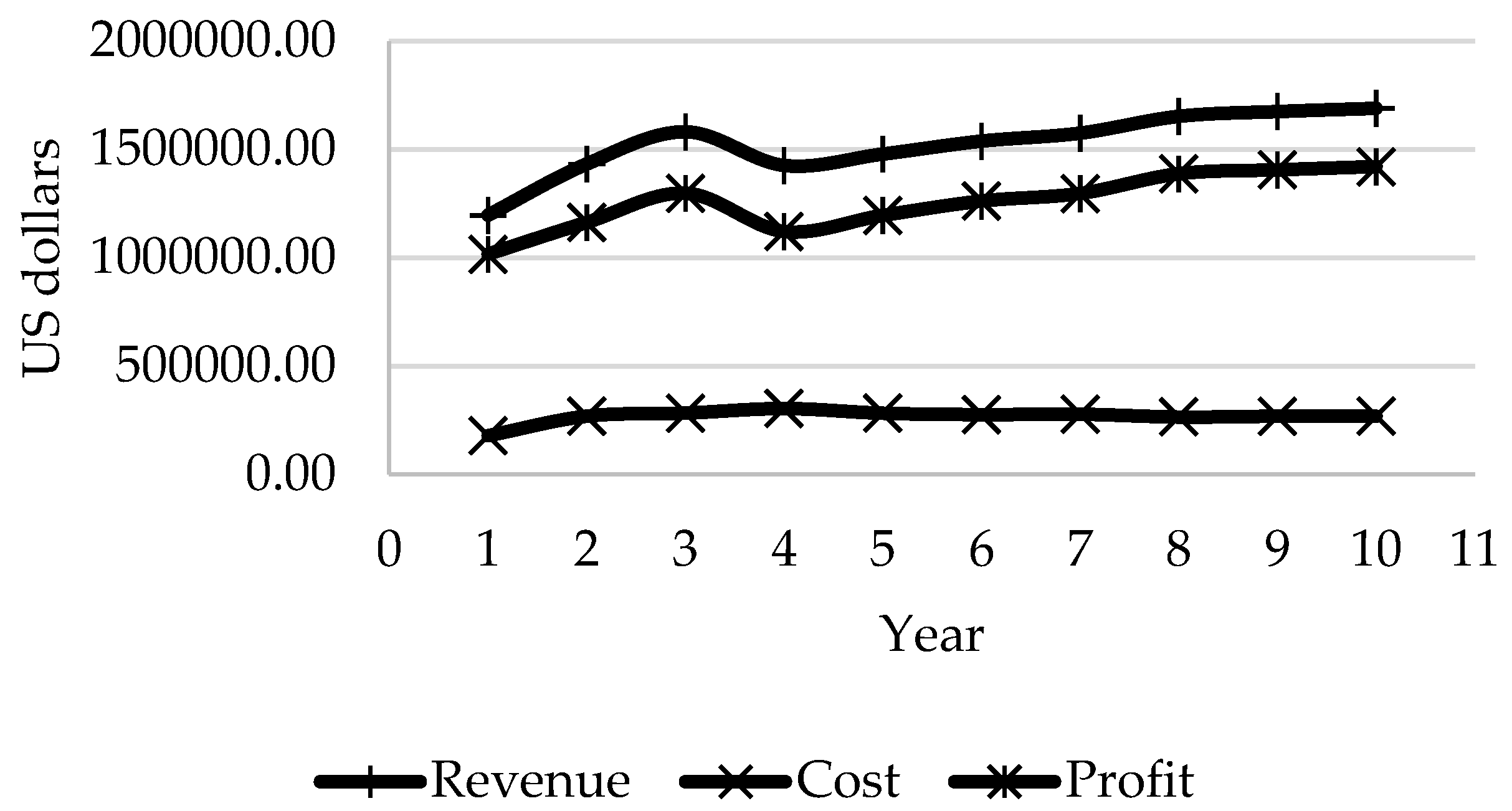
3.2. Objective Function

Max   O = j i s t p j i s t · S T j i s t + j m s t q j m s t · S W M j m s t + j s t r j s t · S B j s t j t c p j t · Y j t j c h t · X j k t 1 j c r t · Z 1 j , k = 10 , t t F t · c L a b f t H i r e t · c L a b p j c b p s t · S B j s t t s j c P N T j i s t · ϵ i j s t k s c w a t e r k s · w k s j s = 2 c l i g h t i n g j s · v j s
The objective of the proposed model is to determine the planting and harvesting decisions that maximize expected profit for the farmers; this is the difference between the total revenue expected from selling to traders (ST), wholesale markets (SWM), and by-product suppliers (SB), and the total costs of planting, truncating, by-product processing, penalty for missing demand, labor, lighting cost, and watering. The notation is presented in Appendix A.

3.3. Constraints

The first category of constraints (2, 3, and 4) is related to resources (land, water, and lighting).
-
Land availability
j k X j k t   L       t
Total of area of each crop j at age k cannot exceed the available land (L).
-
Water restriction
j k X j k s t · w j k s t W s t       t , s
At each tree age k, the amount of water w required per hectare for each crop j is different in season s of year t; this cannot exceed the availability of water. Also, yield decreases if the trees are watered too much.
-
Lighting restrictions
j X j s · v s V s       s
Due to lack of sunlight in the dry seasons (s = 2), a light supplementing method is applied at night. At each tree age k, the requirement of light per hectare for each crop j is different but limited.
Constraints (5) and (6) are for plantation area and yield.
-
Minimum plantation size
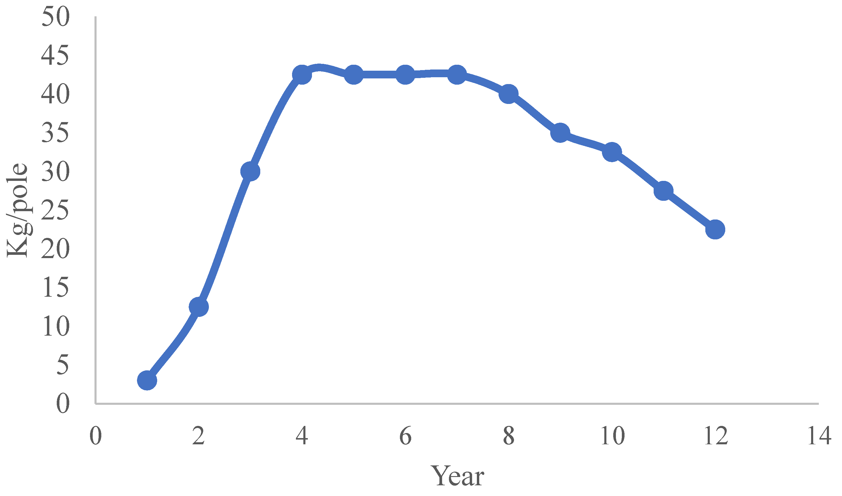
j X j t k u j t       t
Constraint (5) is the lower bound for the planting area for each crop in a given period, which may come from forward contracts. The minimum planting area of each crop u is defined by the planner depending on commitments to customers. The parameter u could be 0 but should be less than the available land L.
-
Yield
i S T j i s t + m S W M j m s t + S B j s t k γ j k s t X j k s t     j , s , t
Constraint (6) ensures that the total harvest is less than the yield (metric tons per hectare) times plantation area (in hectares).
-
Plantation age class balance
The third category of constraints (7–15) is related to the planning structure for agriculture models. The cutting down and replanting of new varieties has been modeled in Catalá [10] for a case study on apple and pear trees.
X j , k , s = 1 , t = X j , k , s = 2 , t       j ,   k ,   t
Constraint (7) ensures that there is no change in the planted area of each crop within a year (i.e., between season 1 and season 2). This is because plantation or truncation decisions are only made at the start of season 1.
The plantation decisions are decided by Y j t . The age of a newly planted fruit tree is always 0. There are two types of truncations: Z 1 j k t , which is optional for a tree of age k = 1 9 and Z 2 j , k = 10 , t which is mandatory for all trees that have reached an age of 10.
X j k s t = Y j t         j ,   k = 1 ,   t = 1
Constraint (8) states that in year 1 only new crops (age class 1) can be planted.
X j k s t = I j , k 1 Z 1 j k t       j ,   k = [ 2 9 ] ,   t = 1
Constraint (9) is similar to constraint 8 and applies only to year 1 but for other age classes (k = 2…9). It states that the plantation area is the inventory of trees of age class k-1 in year 0 less what can be cut down in year 1 after they have aged by 1 year.
X j k s t = I j , k 1 Z 2 j k t       j ,   k = 10 ,   t = 1
Constraint (10) states that age-10-crops that have to be cut down in year 1 while determining the initial plantation area.
X j k s t = Y j , t 1 Z 1 j k t       j ,   k = 1 ,   t > 1
Constraint (11) states that for periods t > 1 in the planning horizon, the plantation area for age class k = 1 is determined by new crop planted the year before less whatever is cut from that new plantation the next year.
X j k s t = X j , k 1 , s , t 1 Z 1 j k t       j ,   10 > k > 1 ,   t > 1
Constraint (12) is for crop ageing for age classes 10 > k > 1. The plantation size in a given year depends on what it was the previous year, less the area cut down optionally.
Z 2 j k t = X j , k 1 , s , t 1         j ,   k = 10 ,   t > 1
Constraint (13) states that all crops of age 9 in a given year t-1 should be cut the next year.
-
Labor constraints
F t + H i r e t P t · j Y j t H t · j X j t R t · j Z j k t = 0       t
Constraints (14) models workforce requirements to plant, cut, and harvest in given year.
F t = M       t
The number of fulltime workers is sometimes a fixed number. If that is the case, the full time complement of workers should be set to that number.
H i r e t N       t
The number of part time workers hired based on requirements of cultivating or harvesting or truncating. However, the number is limited due to budget, as seen in constraint (16).
The last set of constraints, (17) to (19), is for demand satisfaction:
j S T j i s t = d j i s t ϵ j i s t       t , s
Constraint (17) is a soft constraint on trader demands, given that under-shipping to them is allowed.
j S W M j m s t = e j m s t      t , s
Constraint (18) states that the demand of wholesalers should be satisfied.
j S B j t = f t t
Constraint (19) states that the demand of by-products should be satisfied.

4. Case Study

The model for dragon fruit cultivation presented in the previous section was applied using the conditions of an actual dragon fruit plantation in Vietnam. The authors of this study contacted a small growing operation covering an area of about 20 hectares. Data were obtained on dragon fruit prices and demands, planting, replanting, and harvesting costs, labor availability, water and light requirements, species yields, etc. The important issue facing such operations is land management, where farmers need to make decisions on land allocation for different species of dragon fruit over a period of 10 years. The model is intended to allow farming communities to evaluate alternative land allocation and commitment scenarios based on different prices.
As mentioned, farmers are planting two kinds of dragon fruit (white-flesh and red-flesh) on their lands. The price of each crop is different and depends on market demands. The price of the red-skin white-flesh dragon fruit (Crop 1) is stable in season 1 (favorite season) and increases a bit in season 2 (off-season). The price of the red-skin red-flesh dragon fruit (Crop 2) is double because Crop 2 is planted for export to China, where the demand is always good. However, the price of this crop fluctuates highly, relying heavily on Chinese traders. Verbal agreements are usually made between farmers and traders; however farmers could be ruled by the prices set by the traders [40]. In the case of traders cancelling deals, the price drops down dramatically.
The yellow-skin white-flesh dragon fruit (Crop 3) (currently imported from Malaysia) has only recently appeared in the market and has had an extremely high price for the last three years. It is still in great demand because of its sweetness and the curiosity of consumers. Farmers intend to grow Crop 3 trees to cover that demand but have some disadvantages: the plants are novel and disease prone, and yields are just one-third of Crop 1 or Crop 2 (according to the experience of many farmers). However, farmers like to grow all three kinds of dragon fruit, to cover all market demands and hedge their risks against demand and price.
In the baseline scenario, the Crop 1 is the traditional chain for both domestic and export markets with a stable demand, while Crop 2 is only planted for export to China. Crop 3 is cultivated only for the purpose of testing its viability in the consumer market. The model assumes that the demands and selling prices of all crops increase steadily over 10 years.
The land proportion for each type of dragon fruit is proposed to help farmers managing their costs and benefits in planning the combination framework to install various dragon fruits, and also to decide thereafter which dragon fruit category they have to grow within 10 years. The mean values for one year are based on the previous year’s data. Using recent pricing in the Vietnamese market it was found that: (a) the price of Crop 3 is around 10 times higher than the price of Crop 1, and (b) the price of Crop 2 is three times as high as for Crop 1.
After the baseline scenario is completed and analyzed by the proposed model, other scenarios are developed, based on the minimum limit of area for each crop of dragon fruit to plant, and the fluctuations of the prices and market demands. To test how the model adapts to any changes or requirements of dragon fruit production, groups of different expansion scenarios are developed with various assumptions. The model is implemented using open source LP/MIP solver GLPK/GUSEK, that was developed by Free Software Foundation, Inc., Boston, USA, and it is computationally tractable.

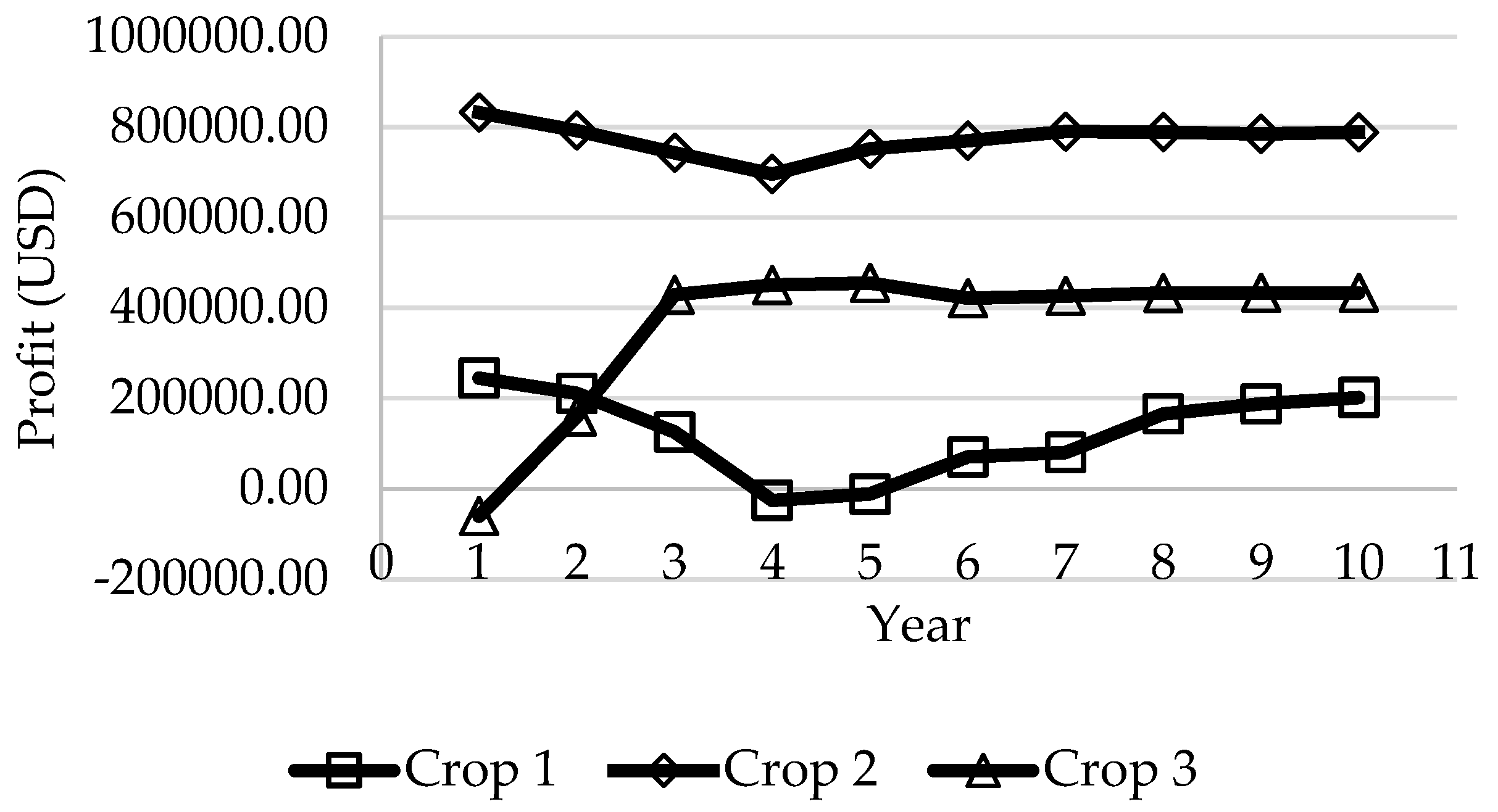
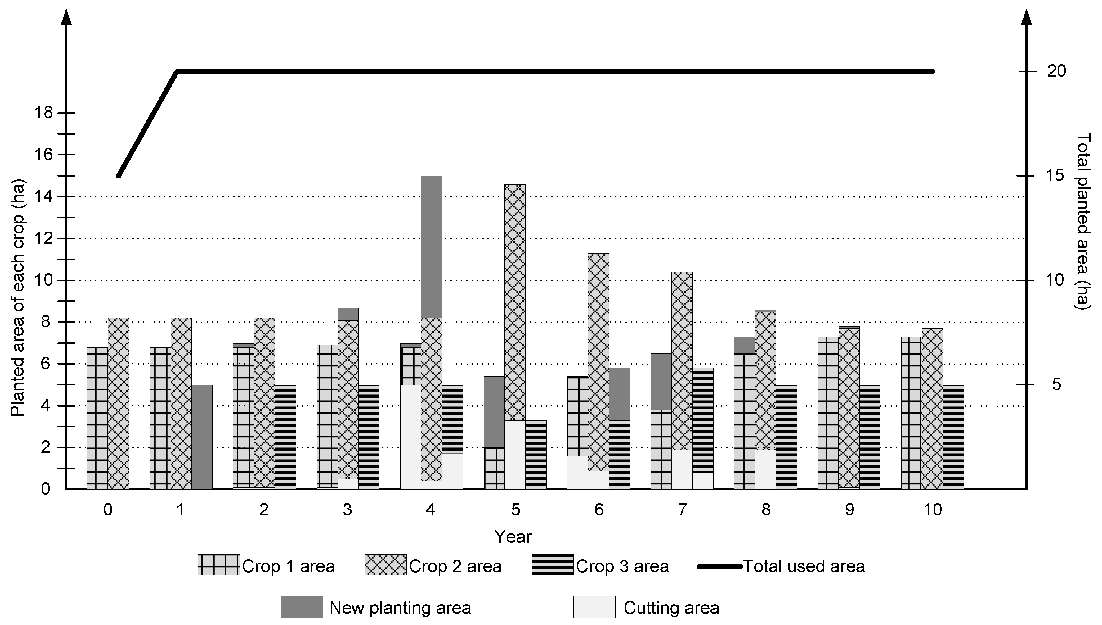
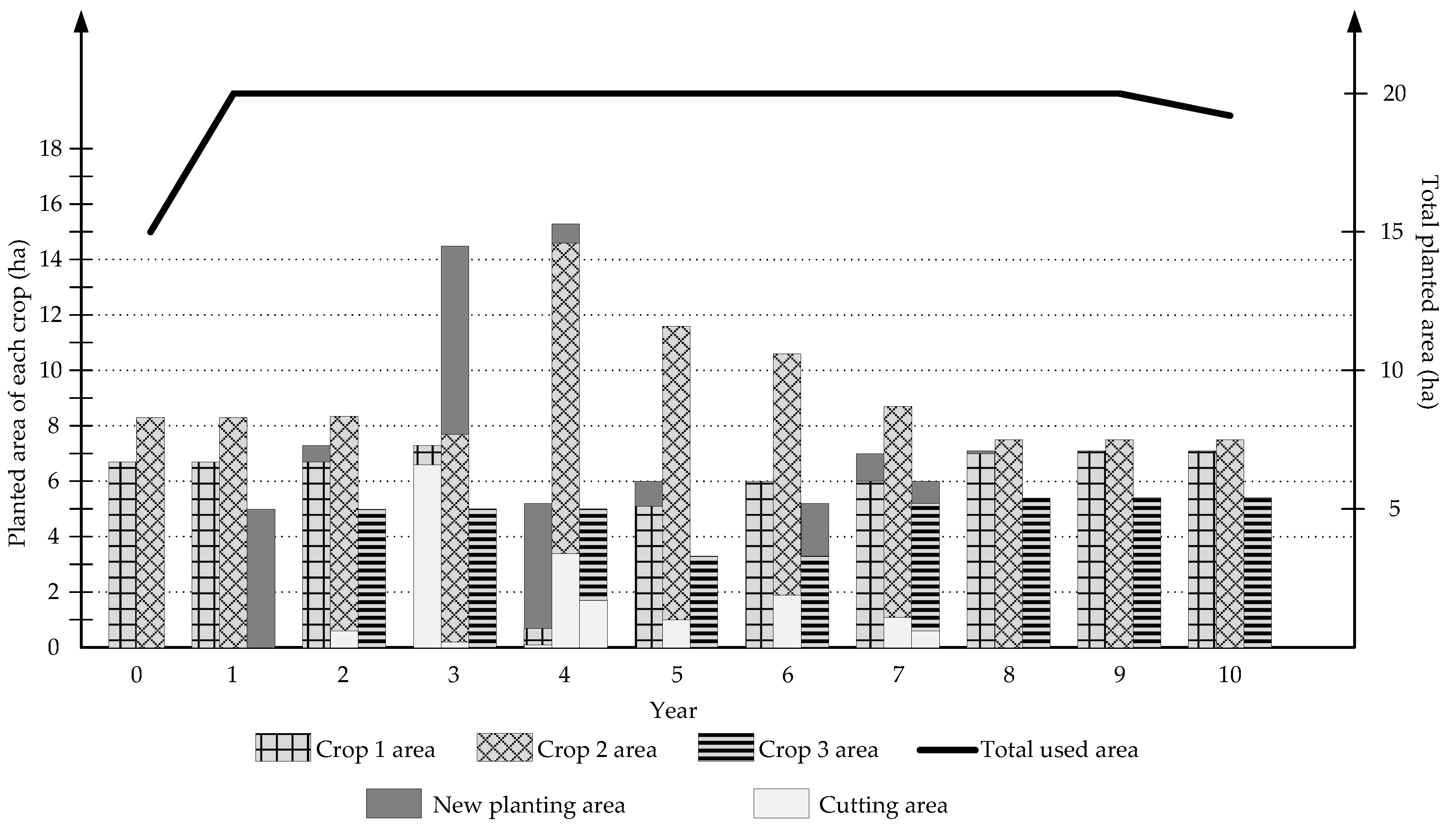
4.1. Baseline Scenario

In this scenario, approximately 15 hectares of Crop 1 and Crop 2 have been planted on 20 hectares of land to meet orders in year 0 (the start of the planning horizon). All initial input values such as yields, prices, demands, labor costs, and resource costs were collected from farmers, market reports, and dragon fruit cultivating guidelines in 2017. Figure 7 shows the typical yield curve of three dragon fruit varieties as a function of tree age [41,43].
It is assumed that all dragon fruits are sold to five traders and five wholesalers. After meeting the needs of all traders and wholesalers, if any amount of Crop 1 is left over, it is sold as a by-product to produce wine and snacks. General information of average yields, demand, and prices of each crop in the current market is show in Table 1:
The results of the baseline scenario are show below:
Figure 8 shows the recommended dragon fruit cultivation allocation to crops on 20 hectares of land over 10 years. Crop 3 is planted primarily to meet demand; the land area allocation of Crop 1 and Crop 2 are relatively constant through the 10 years. We can see that growing new trees and cutting old ones occur on a large area of land from year 3 to year 6; this also affects to the profitability of the farmers. The profit increases rapidly in the first three years due to income from Crop 3. However, it goes down in year 4 because many older Crop 1 and 2 plants are truncated and replaced by new ones. The variations of revenues, profits, and costs are shown in Figure 9. Figure 10 shows the profit of each crop over 10 years.
Building upon the baseline scenario, four different expansion scenarios are proposed with assumptions about changes to prices or demands, price fluctuation with a probability factor, and the initial plantation. All scenarios are described briefly in Appendix B (Table A1).

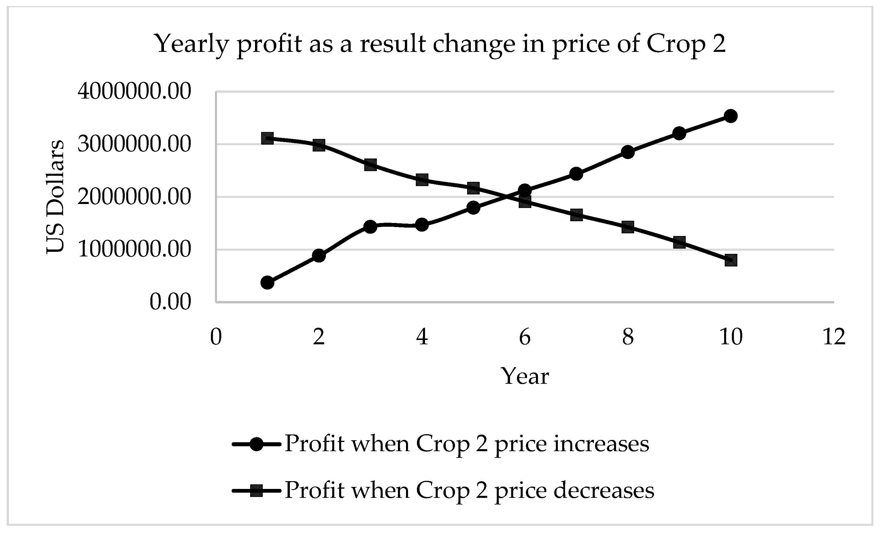
4.2. Changes to Price of Crop 2

In this scenario, the price of Crop 2 is considered increasing or decreasing linearly within the range of 0.5 US$ (Crop 1 price) and 5 US$ (Crop 3 price). The other information is the same as in the baseline scenario. The cultivation changes for each crop when the price of Crop 2 changes in two cases are shown below:
We can see effect the price of Crop 2 price in Figure 11 and Figure 12. The total profits are also affected when the prices are changed (Figure 13).

4.3. Changing Demands

In this scenario, market demand variations are considered. It is assumed that the need of the market rises for all crops. The following cases are considered: Crop 3 demand increases four-fold and the demand for all crops required increases by 20%, 40%, and 80%, respectively, based on the baseline scenario demand. Other information is unchanged.

4.3.1. Crop 3 Demand Increases Four-Fold

In this case, it is supposed that the yellow-skin white-flesh dragon fruit is popular, so that the farmers have more orders from traders and wholesalers. The areas of new planting or cutting of the dragon fruit trees are shown below:
Figure 14 shows us that with the rising demand along with its high selling price, Crop 3 is produced on most of the current planting area. On the other hand, Crop 2 is grown on the small remaining land and Crop 1 is cut off completely in year 2.

4.3.2. All Crop Demands Increasing by a Fixed Percentage

This case is slightly different from the case 2.3.1, and all crop demands increase by 20%, 40%, and 80% respectively over the baseline scenario demand. Other data are the same. The changes in plantation allocation for each case is shown in Figure 15, Figure 16 and Figure 17 below:
We can see that if the needs of all crops are increased, only crops that are more profitable are grown. Therefore, Crop 2 and 3 are prioritized for planting. The profit of each case is summarized in Figure 18. In general, the higher the demand is, the more the dragon fruit grower’s revenue is.

4.4. Crop 3 Selling Price with a Probability Factor

Currently, the bulk of Crop 3 in the market is imported. If it could be produced domestically, this demand would be less dependent on imports and could relieve price fluctuations. For this case, a probability factor is considered in the selling price. It is assumed three Crop 3 price scenarios of $1, $5, or $10 occurs in each year of the planning period of 10 years. The probability for each price is assumed be a discrete combination of 0.2, 0.2, and 0.6 for a total of 1.0 for the three price scenarios. The changes to the plantation for each case is presented below:
Figure 19, Figure 20 and Figure 21 show that the higher the most probable price of Crop 3, the greater the land allocated to it in the first year. The area of Crop 3 for each case is 5 ha, 4.7 ha, and 4 ha, respectively. In addition, the change in area of cultivating land is also affected: the lower the most probable price, the higher the changeover to other crops. This can be observed in the 10-year profit projections (Figure 22).

4.5. Land Restriction

This scenario was suggested by the farmers who want to not only have a stable plantation size for each crop, but also supply all three varieties of dragon fruits to the market. They would like to use 50%, 35%, and 15% of their land to produce Crop 1, Crop 2, and Crop 3, respectively, and this is in some sense a risk-hedging strategy. The cultivation activities (Figure 23) and the profit–cost relationship (Figure 24) for a 10-year horizon are shown below:
To ensure both the stability of area for each crop and the amount supplied to the market, farmers should re-vitalize the trees every few years (cutting old plants and planting new ones), especially in the 4th year.

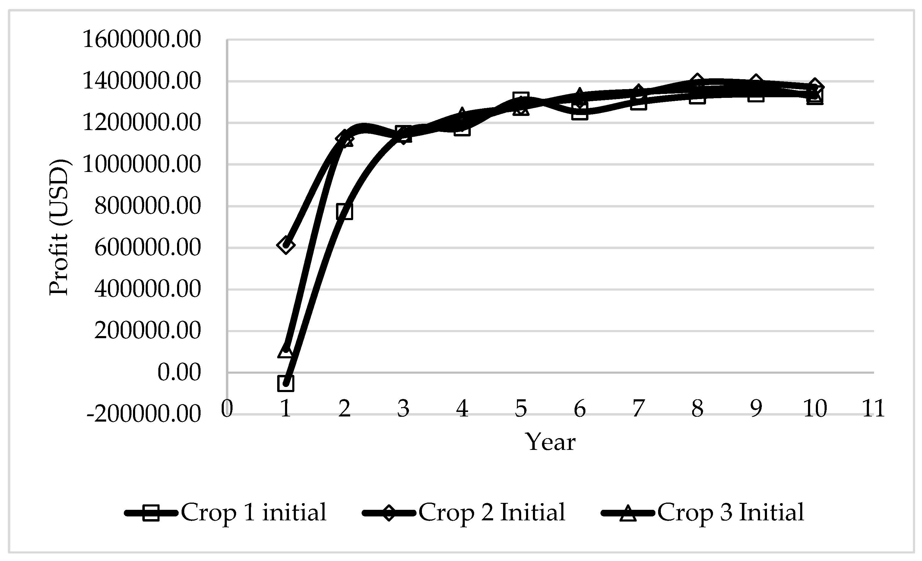
4.6. Influence of the Initial Plantation Conditions

In addition to the mentioned variables above, such as customer demand and selling prices, the initial crop status of the arable land is also considered to determine its influence on the changes in planting area. Based on the result of the baseline scenario, two sub-scenarios are proposed to look at the effect of the variety of the initial crop and the age of the initial crop. In the first sub-scenario set, it is supposed that all initial area has been allocated to only one of the three crops (Crop 1 or Crop 2 or Crop 3). In the second sub-scenario set, only the initial land for Crop 1 is considered, with different ages (age 1, age 3, and age 5) in year 0. Other data is the same as in the baseline scenario.

4.6.1. Initial Plantation with Only One Kind of Crop

According to results of the baseline scenario, the initial area that is used in year 0 is 15.3 hectares. It is assumed that only one crop has been planted on that area in year 0. Figure 25, Figure 26 and Figure 27 show the cultivation activities for each case.
Although the initial land varies across these sub scenarios, Crop 2 is still the most planted over the next 10 years. The profit for the case where the entire plantation consists of Crop 2 is also the highest, as shown in Figure 28 below:

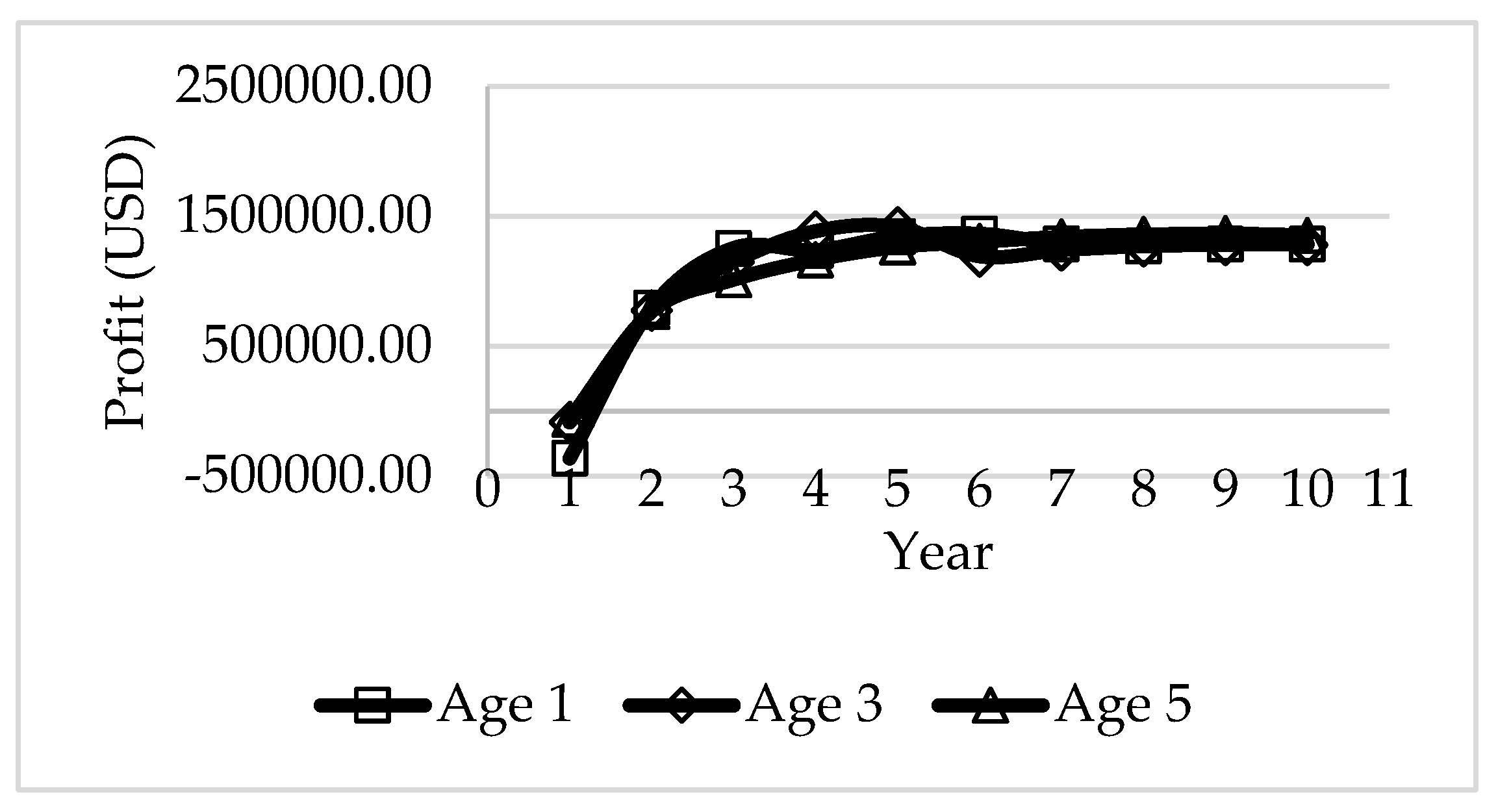
4.6.2. The Initial Crop Allocation with Different Crop 1 Ages

In this case, it is assumed that the initial crop allocation is only for Crop 1. However, it is assumed that the age is 1, 3, or 5 in year 0. The optimal crop allocation over the next 10 years is shown in Figure 29, Figure 30 and Figure 31.
We can see that the young Crop 1 (age 1) is truncated more than the grown one (age 3 or age 5). Similar to trends observed earlier, after Crop 1 area is reduced, most of the remaining land is prioritized for Crop 2, which has the most revenue because of its high demand. The profits for all three cases are shown in Figure 32.

4.7. Discussion

Throughout scenarios and cases above, summarized in Table 2, we can see that the dragon fruit growers earn more profit if they prioritize planting the varieties for which both demand and selling price are high. This is the case for Crop 2 which has a very high demand and its price is only lower than the price of Crop 3. In contrast, although the price of Crop 3 is the highest, due to lower demand and yield, it is not prioritized in the solutions. Finally, the selling price of Crop 1 is the lowest; therefore, it is replaced by other varieties when the demands or prices of the other two crops increase. Table 2 summarizes the profits for each of the scenarios.

5. Conclusions

A deterministic model is proposed in this paper to assist dragon fruit farmers with their decision making on crop allocation for different species of dragon fruits. Consequently, it can provide them a long-term overview through groups of production scenarios that could occur, such as (1) price changes (e.g., price of the red-skin red-flesh dragon fruit—Crop 2); (2) changes in demand (e.g., demand of the yellow-skin white-flesh dragon fruit—Crop 3); (3) requirements for land restrictions for each type of crop, and (4) the influence of the initial state. All scenarios are variants from a baseline scenario of the actual dragon fruit production conditions in Vietnam intended to provide insights. Results obtained from this model confirmed that the Crop 2 should be prioritized for planting.
The model presented in this paper represents a first step towards a comprehensive quantitative approach for decision making in dragon fruit cultivation in Vietnam. The model works well with some scenarios showing relationships of input factors (demands, prices, and costs) and output decisions (plantation area of crops) over a 10-year period. This is evident in the cases of “no limit plantation area” of all scenarios: the crop is grown if its demand and price increase, or it is cut down when its demand is low and its price drops. For a specific crop, the old plants are replaced by new ones if its yield is too low due to age.
The proposed model is a meaningful tool for managers and farmers to have a holistic view for long term planning with the goal of maximizing profits. It helps decide which varieties to plant proactively based on demand and price scenarios.
As with other fresh fruit supply chains, the dragon fruit chain faces challenges due to inherent uncertainties such as demands, price, and yield. This is the main limitation of the deterministic approach. Therefore, future research to deal with randomness and uncertainty for dragon fruit cultivation could involve stochastic programming [44,45,46] or robust optimization [47]. The approach can be generalized to other similar fresh fruit supply chains.

Author Contributions

Conceptualization: T.-D.N., U.V., T.N.-Q.; Data curation: T.-D.N., T.N.-Q.; Format analysis: T.-D.N., U.V., T.N.-Q.; Funding acquisition: T.N.-Q.; Investigation: T.-D.N., U.V.; Methodology: T.-D.N., U.V., T.N.-Q.; Supervision: U.V., T.N.-Q., C.D., M.A.; Validation: T.-D.N., U.V., T.N.-Q., C.D., M.A.; Visualization: C.D., M.A.; Writing—original draft: T.-D.N., U.V., T.N.-Q.; Writing—review & editing: T.-D.N., U.V., T.N.-Q., C.D., M.A. All authors have read and agreed to the published version of the manuscript.

Funding

This research was funded by the Vietnam International Education Development (VIED).

Acknowledgments

The first author acknowledges the Vietnam International Education Development (VIED) via the 911 research scholarship program as well as Vietnamese colleagues, collaborators, and the farmers from Binh Thuan, Vietnam for the data collection.

Conflicts of Interest

The authors have no conflicting financial or other interests.

Nomenclature

DCDistribution Centers
DFDragon fruit
FFSCFresh Fruit Supply Chain
FSCFruit Supply Chain
GLPKGNU Linear Programming Kit
GUSEKGLPK Under Scite Extended Kit
LPLinear Programming
MIPMixed Integer Programming
VIEDThe Vietnam International Education Development

Appendix A

Indices:
tTime periods
kAge classes in the plantation, each representing a two-year period
sHarvesting season (1 for wet, 2 for dry)
jDifferent species of dragon fruit
iTraders
mWholesale markets (WM)
bBy-product
Parameters:
LAmount of land available
w k s Water required per hectare for crop j of age class k in season s
v j s Lighting required per hectare for crop j in season s
WsWater restriction in season
VsLighting restriction in season
u j t Minimum planting area per crop j in period t
γ j k s t Yield in kgs per hectare of crop j belonging to age class k in season s
p j i s t Price per kg of crop j for trader i in season s of period t
q j m s t Price per kg of crop j for wholesaler m in season s of period t
r s t Price per kg of byproducts (e.g., wine) in period t
d i j s t Demand of trader i for crop j in season s of period t
e m j s t Demand of wholesale market m for crop j in season s of period t
f t Demand for byproducts (e.g., wine) in period t
P t Number of workers needed to plant one hectare
H t Number of workers needed to harvest one hectare
R t Number of workers needed to cut one hectare
MMaximum number of fixed workers in a period
NMaximum number of part-time workers in a period
I j k Initial area of crop j of age class k
Cost parameters:
c p t Cost per hectare of planting in period t
c h t Cost per hectare of harvesting in period t
c r t Cost per hectare of cut in period t
c b p t Cost per kg of processing (e.g. wine)
c L a b f Cost of fixed workers per period
c L a b p Labor cost of part-time workers per period
c P N T j i s t Penalty for not meeting demand per kg of crop j for trader i
in season s of period t
c w a t e r k s Cost of required water per hectare for crop j of age class k
in season s
c l i g h t i n g j s Cost of required light per hectare for crop j in season s
Variables:
X j k t Plantation area of crop j in period t of age class k
S T j i s t Quantity of crop j shipped to trader i in season s of period t
ϵ i j s t Quantity of crop j under shipped to trader i in season s of period t
S W M j m s t Quantity of crop j shipped to WM m in season s of period t
S B j s t Quantity of crop j harvested for by-products (e.g. wine) in season s of
period t
F t Number of fixed workers in t
H i r e t Part-time workers hired in period t
Y j t Area of crop j planted in period t
Z 1 j k t Area of crop j of age class k cut optionally in period t
Z 2 j k t Area of crop j of age class k = 10 that must be cut in period t
Z j t Area of crop j of age class k cut in period t in total

Appendix B

Table A1. Summary of scenarios with their characteristics.
ScenarioSituation (Sub-Scenario or Case)Limit of Planting Area for Each CropDescriptions
Baseline scenario No limit for each cropDemands and prices unchanged within 10 years
Changes in price of Crop 21No limit for each cropThe price increasing gradually within 10 years
2No limit for each cropThe price decreasing gradually within 10 years
Changes in demands1No limit for each cropDemand of Crop 3 increasing 4 times
2No limit for each cropDemands of all crops increasing 20%
3No limit for each cropDemands of all crops increasing 40%
4No limit for each cropDemands of all crops increasing 80%
Crop 3 selling price with probability factor1No limit for each crop0.2 for $1, 0.2 for $5, and 0.6 for $10
2No limit for each crop0.2 for $1, 0.6 for $5, and 0.2 for $10
3No limit for each crop0.6 for $1, 0.2 for $5, and 0.2 for $10
Land restriction 50% for Crop 1, 35% for Crop 2, 15% for Crop 3Demands and prices unchanged within 10 years
Influence of initial landCrop 1No limit for each cropAll initial land used for Crop 1. Demands and prices unchanged within 10 years
Crop 2No limit for each cropAll initial land used for Crop 2. Demands and prices unchanged within 10 years
Crop 3No limit for each cropAll initial land used for Crop 2. Demands and prices unchanged within 10 years
Crop 1—Age 1No limit for each cropAll initial land used for Crop 1 at age 1. Demands and prices unchanged within 10 years
Crop 1—Age 3No limit for each cropAll initial land used for Crop 1 at age 3. Demands and prices unchanged within 10 years
Crop 1—Age 5No limit for each cropAll initial land used for Crop 1 at age 5. Demands and prices unchanged within 10 years

References

  1. Ahumada, O.; Villalobos, J.R. Application of planning models in the agri-food supply chain: A review. Eur. J. Oper. Res. 2009, 196, 1–20. [Google Scholar] [CrossRef]
  2. Hamer, P.J. A decision support system for the provision of planting plans for Brussels sprouts. Comput. Electron. Agric. 1994, 11, 97–115. [Google Scholar] [CrossRef]
  3. Maia, L.O.A.; Lago, R.A.; Qassim, R.Y. Selection of postharvest technology routes by mixed-integer linear programming. Int. J. Prod. Econ. 1997, 49, 85–90. [Google Scholar] [CrossRef]
  4. Ferrer, J.C.; Mac Cawley, A.; Maturana, S.; Toloza, S.; Vera, J. An optimization approach for scheduling wine grape harvest operations. Int. J. Prod. Econ. 2007, 112, 985–999. [Google Scholar] [CrossRef]
  5. Widodo, K.H.; Nagasawa, H.; Morizawa, K.; Ota, M. A periodical flowering–harvesting model for delivering agricultural fresh products. Eur. J. Oper. Res. 2006, 170, 24–43. [Google Scholar] [CrossRef]
  6. Caixeta-Filho, J.V. Orange harvesting scheduling management: A case study. J. Oper. Res. Soc. 2006, 57, 637–642. [Google Scholar] [CrossRef]
  7. Itoh, T.; Ishii, H.; Nanseki, T. A model of crop planning under uncertainty in agricultural management. Int. J. Prod. Econ. 2003, 81, 555–558. [Google Scholar] [CrossRef]
  8. Ten Berge, H.; Van Ittersum, M.; Rossing, W.; Van de Ven, G.; Schans, J. Farming options for The Netherlands explored by multi-objective modelling. Eur. J. Agron. 2000, 13, 263–277. [Google Scholar] [CrossRef]
  9. Rantala, J. Optimizing the supply chain strategy of a multi-unit Finnish nursery company. Silva Fenn. 2004, 38, 203–215. [Google Scholar] [CrossRef] [Green Version]
  10. Catalá, L.P.; Durand, G.A.; Blanco, A.M.; Bandoni, J.A. Mathematical model for strategic planning optimization in the pome fruit industry. Agric. Syst. 2013, 115, 63–71. [Google Scholar] [CrossRef]
  11. Rocco, C.D.; Morabito, R. Production and logistics planning in the tomato processing industry: A conceptual scheme and mathematical model. Comput. Electron. Agric. 2016, 127, 763–774. [Google Scholar] [CrossRef]
  12. Grillo, H.; Alemany, M.; Ortiz, A.; Fuertes-Miquel, V. Mathematical modelling of the order-promising process for fruit supply chains considering the perishability and subtypes of products. Appl. Math. Model. 2017, 49, 255–278. [Google Scholar] [CrossRef]
  13. Ahumada, O.; Villalobos, J.R. Operational model for planning the harvest and distribution of perishable agricultural products. Int. J. Prod. Econ. 2011, 133, 677–687. [Google Scholar] [CrossRef]
  14. Ahumada, O.; Villalobos, J.R. A tactical model for planning the production and distribution of fresh produce. Ann. Oper. Res. 2011, 190, 339–358. [Google Scholar] [CrossRef]
  15. Amorim, P.; Günther, H.O.; Almada-Lobo, B. Multi-objective integrated production and distribution planning of perishable products. Int. J. Prod. Econ. 2012, 138, 89–101. [Google Scholar] [CrossRef]
  16. Masini, G.L.; Blanco, A.M.; Petracci, N.; Bandoni, J.A. Supply chain tactical optimization in the fruit industry. Process Syst. Eng. Supply Chain Optim. 2007, 4, 121–172. [Google Scholar]
  17. Jena, S.D.; Poggi, M. Harvest planning in the Brazilian sugar cane industry via mixed integer programming. Eur. J. Oper. Res. 2013, 230, 374–384. [Google Scholar] [CrossRef]
  18. Willis, C.; Hanlon, W. Temporal Model for Long-Run Orchard Decisions. Can. J. Agric. Econ. 1976, 24, 17–28. [Google Scholar] [CrossRef]
  19. González-Araya, M.C.; Soto-Silva, W.E.; Espejo, L.G.A. Harvest Planning in Apple Orchards Using an Optimization Model. In Handbook of Operations Research in Agriculture and the Agri-Food Industry; Springer: New York, NY, USA, 2015; pp. 79–105. [Google Scholar]
  20. Starbird, S.A. Optimal loading sequences for fresh-apple storage facilities. J. Oper. Res. Soc. 1998, 39, 911–917. [Google Scholar] [CrossRef]
  21. Hester, S.M.; Cacho, O. Modelling apple orchard systems. Agric. Syst. 2003, 77, 137–154. [Google Scholar] [CrossRef] [Green Version]
  22. Blanco, A.; Masini, G.; Petracci, N.; Bandoni, J. Operations management of a packaging plant in the fruit industry. J. Food Eng. 2005, 70, 299–307. [Google Scholar] [CrossRef]
  23. Nadal-Roig, E.; Plà-Aragonés, L.M. Optimal Transport Planning for the Supply to a Fruit Logistic Centre. In Handbook of Operations Research in Agriculture and the Agri-Food Industry; Springer: New York, NY, USA, 2015; pp. 163–177. [Google Scholar]
  24. Cittadini, E.D.; Lubbers, M.; de Ridder, N.; Van Keulen, H.; Claassen, G. Exploring options for farm-level strategic and tactical decision-making in fruit production systems of South Patagonia, Argentina. Agric. Syst. 2008, 98, 189–198. [Google Scholar] [CrossRef]
  25. Arnaout, J.P.M.; Maatouk, M. Optimization of quality and operational costs through improved scheduling of harvest operations. Int. Trans. Oper. Res. 2010, 17, 595–605. [Google Scholar] [CrossRef]
  26. Vitoriano, B.; Ortuño, M.T.; Recio, B.; Rubio, F.; Alonso-Ayuso, A. Two alternative models for farm management: Discrete versus continuous time horizon. Eur. J. Oper. Res. 2003, 144, 613–628. [Google Scholar] [CrossRef]
  27. Van Der Vorst, J.G.; Tromp, S.O.; van der Zee, D.J. Simulation modelling for food supply chain redesign; integrated decision making on product quality, sustainability and logistics. Int. J. Prod. Res. 2009, 47, 6611–6631. [Google Scholar] [CrossRef]
  28. Banaeian, N.; Omid, M.; Ahmadi, H. Greenhouse strawberry production in Iran, efficient or inefficient in energy. Energy Effic. 2012, 5, 201–209. [Google Scholar] [CrossRef]
  29. Blackburn, J.; Scudder, G. Supply chain strategies for perishable products: The case of fresh produce. Prod. Oper. Manag. 2009, 18, 129–137. [Google Scholar] [CrossRef]
  30. Miller, W.; Leung, L.; Azhar, T.; Sargent, S. Fuzzy production planning model for fresh tomato packing. Int. J. Prod. Econ. 1997, 53, 227–238. [Google Scholar] [CrossRef]
  31. Ahumada, O.; Villalobos, J.R.; Mason, A.N. Tactical planning of the production and distribution of fresh agricultural products under uncertainty. Agric. Syst. 2012, 112, 17–26. [Google Scholar] [CrossRef]
  32. Nielsen, I. Plant Resources of Tropical Africa 2: Vegetables Grubben, G.J.H., Denton, O.A., Eds. Nord. J. Bot. 2004, 23, 298. [Google Scholar] [CrossRef]
  33. Lambert, G.F.; Lasserre, A.A.A.; Ackerman, M.M.; Sánchez, C.G.M.; Rivera, B.O.I.; Azzaro-Pantel, C. An expert system for predicting orchard yield and fruit quality and its impact on the Persian lime supply chain. Eng. Appl. Artif. Intel. 2014, 33, 21–30. [Google Scholar] [CrossRef]
  34. Defraeye, T.; Nicolai, B.; Kirkman, W.; Moore, S.; van Niekerk, S.; Verboven, P.; Cronjé, P. Integral performance evaluation of the fresh-produce cold chain: A case study for ambient loading of citrus in refrigerated containers. Postharvest Biol. Technol. 2016, 112, 1–13. [Google Scholar] [CrossRef]
  35. Wu, W.; Defraeye, T. Identifying heterogeneities in cooling and quality evolution for a pallet of packed fresh fruit by using virtual cold chains. Appl. Therm. Eng. 2018, 133, 407–417. [Google Scholar] [CrossRef]
  36. Raut, R. Improvement in the Food Losses in Fruits and Vegetable Supply Chain-A Perspective of Cold Third-Party Logistics Approach. Oper. Res. Perspect. 2019, 6, 100117. [Google Scholar] [CrossRef]
  37. Wu, W.; Beretta, C.; Cronje, P.; Hellweg, S.; Defraeye, T. Environmental trade-offs in fresh-fruit cold chains by combining virtual cold chains with life cycle assessment. Appl. Energy 2019, 254, 113586. [Google Scholar] [CrossRef]
  38. Zhao, X.; Xia, M.; Wei, X.; Xu, C.; Luo, Z.; Mao, L. Consolidated cold and modified atmosphere package system for fresh strawberry supply chains. LWT 2019, 109, 207–215. [Google Scholar] [CrossRef]
  39. Luong, N.T.L.; Nguyen, M.C. Increasing Market Access of Selected Tropical Fruit Through Value Chain Improvements in Vietnam; Food and Fertilizer Technology Center for the Asian and Pacific Region: Taipei, Taiwan, 2015; Available online: http://www.fftc.agnet.org/library.php?func=view&style=type&id=20150805092541 (accessed on 9 July 2017).
  40. AXIS Research. Report on Value Chain of Dragon Fruit of Binh Thuan Province. 2009. Report No.9. Retrieved from Information Center for Agriculture and Rural development, Vietnam (Agroinfo). Available online: http://agro.gov.vn/images/2007/05/Dragon_Fruit_in_BT(E).pdf (accessed on 21 May 2015).
  41. Hai, D.H. Vietnamese Dragonfruit. The Edible Plants in Vietnam. Available online: https://www.edibleplantsinvietnam.com/vietnamese-dragon-fruit-thanh-long.html (accessed on 9 July 2017).
  42. Miller, T.C. Hierarchical Operations and Supply Chain Planning; Springer-Verlag: London, UK, 2002; ISBN 978-1-4471-1110-8. [Google Scholar]
  43. Kiet, Mr.; Cuoc, Mr.; Manh, Mr.; Binh Thuan, Vietnam. Personal communication, 2017.
  44. Birge, J.R.; Louveaux, F. Introduction and Examples. In Introduction to Stochastic Programming, 2nd ed.; Springer: New York, NY, USA, 2011; ISBN 978-1-4614-0237-4. [Google Scholar]
  45. Darby-Dowman, K.; Barker, S.; Audsley, E.; Parsons, D. A two-stage stochastic programming with recourse model for determining robust planting plans in horticulture. J. Oper. Res. Soc. 2000, 51, 83–89. [Google Scholar] [CrossRef]
  46. Kazaz, B. Production planning under yield and demand uncertainty with yield-dependent cost and price. Manuf. Serv. Oper. Manag. 2004, 6, 209–224. [Google Scholar] [CrossRef]
  47. Ben-Tal, A.; Ghaoui, L.E.; Nemirovski, A. Robust optimization. In Applied Mathematics; Princeton University Press: Princeton, NJ, USA, 2009; ISBN 978-0-691-14368-2. [Google Scholar]
Figure 1. Dragon fruit trees blossoming (left) and fruiting (right) in June–July. Photos taken in 2016 in Binh Thuan province, Vietnam.
Agriengineering 02 00001 g001
Figure 2. Simplified dragon fruit supply chain [40].
Agriengineering 02 00001 g002
Figure 3. Typical dragon fruit yield as a function of tree age.
Agriengineering 02 00001 g003
Figure 4. Species of dragon fruit planted in Vietnam [41].
Agriengineering 02 00001 g004
Figure 5. Dragon fruit production calendar in Vietnam.
Agriengineering 02 00001 g005
Figure 6. Example of a hierarchical planning schematic.
Agriengineering 02 00001 g006
Figure 7. Yields of three dragon fruit varieties [41,43].
Agriengineering 02 00001 g007
Figure 8. Baseline model result.
Agriengineering 02 00001 g008
Figure 9. Revenue, profit, and cost of the baseline scenario for the 10-year horizon.
Agriengineering 02 00001 g009
Figure 10. Profit of each crop.
Agriengineering 02 00001 g010
Figure 11. Plantation allocation when Crop 2 price increases.
Agriengineering 02 00001 g011
Figure 12. Plantation allocation when Crop 2 price decreases.
Agriengineering 02 00001 g012
Figure 13. Effect of changes in Crop 2 price on profit.
Agriengineering 02 00001 g013
Figure 14. Plantation allocation when Crop 3 demand increases four-fold.
Agriengineering 02 00001 g014
Figure 15. Plantation allocation when all crop demands increase by 20%.
Agriengineering 02 00001 g015
Figure 16. Plantation allocation when all crop demands increase by 40%.
Agriengineering 02 00001 g016
Figure 17. Plantation allocation when all crop demands increase by 80%.
Agriengineering 02 00001 g017
Figure 18. Profit for each case of increasing demand.
Agriengineering 02 00001 g018
Figure 19. Plantation allocation with probability combinationof prices$1 (0.2)–$5 (0.2)–$10 (0.6).
Agriengineering 02 00001 g019
Figure 20. Plantation allocation with probability combination of prices $1 (0.2)–$5 (0.6)–$10 (0.2).
Agriengineering 02 00001 g020
Figure 21. Plantation allocation with probability combinationof prices $1 (0.6)–$5 (0.2)–$10 (0.2).
Agriengineering 02 00001 g021
Figure 22. Profit for each case in scenario 2.4.
Agriengineering 02 00001 g022
Figure 23. Plantation allocation for land restriction scenario.
Agriengineering 02 00001 g023
Figure 24. Revenue, profit, and cost in 10 years.
Agriengineering 02 00001 g024
Figure 25. Plantation allocation if the initial plantation only has Crop 1.
Agriengineering 02 00001 g025
Figure 26. Plantation allocation if the initial plantation only has Crop 2.
Agriengineering 02 00001 g026
Figure 27. Plantation allocation if the initial plantation only has Crop 3.
Agriengineering 02 00001 g027
Figure 28. The profit of the three cases of the initial land allocation.
Agriengineering 02 00001 g028
Figure 29. Plantation allocation if the initial land is only for Crop 1 at age 1.
Agriengineering 02 00001 g029
Figure 30. Plantation allocation if the initial land is only for Crop 1 at age 3.
Agriengineering 02 00001 g030
Figure 31. Plantation allocation if the initial land is only for Crop 1 at age 5.
Agriengineering 02 00001 g031
Figure 32. The profits for the three cases of initial land allocation to Crop 1 for different ages.
Agriengineering 02 00001 g032
Table 1. General information for the model [43].
Average YieldAverage DemandAverage Price
Crop 115300.5 US$
Crop 214301.5 US$
Crop 3555 US$
Table 2. Summary of the profitability of the various scenarios.
ScenarioSub-ScenarioLimit on Plantation Area for Each CropProfit
Baseline scenario No limit for each cropUSD 12,576,086.80
Changes in price of Crop 21No limit for each cropUSD 20,089,622.07
2No limit for each cropUSD 20,116,237.86
Changes in demands1No limit for each cropUSD 16,815,478.39
2No limit for each cropUSD 13,932,145.96
3No limit for each cropUSD 15,166,044.33
4No limit for each cropUSD 15,740,093.18
Crop 3 selling price with probability factor1No limit for each cropUSD 14,438,789.39
2No limit for each cropUSD 12,745,440.97
3No limit for each cropUSD 11,415,607.18
Land restriction 50% for Crop 1, 35% for Crop 2, 15% for Crop 3USD 9,963,130.32
Influence of initial landCrop 1No limit for each cropUSD 10,921,697.80
Crop 2No limit for each cropUSD 12,182,762.60
Crop 3No limit for each cropUSD 11,630,711.50
Crop 1—Age 1No limit for each cropUSD 10,763,932.06
Crop 1—Age 3No limit for each cropUSD 10,907,367.04
Crop 1—Age 5No limit for each cropUSD 10,879,376.28

