1. Introduction
As natural hazards, tsunamis are considered amongst the most potentially devastating phenomena [
1]. From the mid-nineteenth century to today, advances in technology have expanded the possibilities for the development of preventive safety measures, laying the groundwork for warning operations known as tsunami early warning systems (TEWS). TEWS provide real-time information on the occurrence and characteristics of a seismic event and enable the launching of corresponding action and/or evacuation plans if the alert level so indicates. These systems are composed of quite different elements, from physical seismic and tsunami sensors to empirical relationships derived from historical records and communication and actuation organisations.
An important aspect of the warning process is the estimation of arrival times, wave height and run-up, which have recently been enhanced through tsunami-wave simulation codes [
2,
3]. The events in Sumatra (2004) and Japan (2011) have prompted the need to deepen our knowledge of the phenomenom of tsunamis in order to design adequate preventive measures. For example, some measures for tsunami risk reduction have focused on the construction of artificial or natural structures near to the shore [
4,
5]. However, the high economic impact of the construction of physical barriers, in addition to its doubtful reliability when facing large events [
4], has made them controversial. In this example and many others, numerical simulations appear to be an essential tool for tsunami impact studies [
6]. In recent years, tsunami modeling tools have been significantly enhanced; the precision of the numerical methods have increased, whilst computing times have drastically decreased [
7]. TEWS is a tsunami hazard management tool that focuses on the most relevant element to protect, that of human life. However, TEWS cannot prevent property damage, nor do they help to mitigate the aftermath of the tsunami. Therefore, it is a concern, and a challenge, to provide stakeholders with the best possible tools to understand and quantify the damage caused by tsunamis. One of these stakeholders is the insurance sector and in this paper we present numerical modeling and simulation as a tool to quantify the impact of tsunamis. The final objective of the long-term project with the insurance sector in Spain is to estimate the maximum economic cost of a natural hazard of this type that can affect any Spanish coastal area.
In the literature, many authors have employed numerical models to simulate seismic-triggered tsunamis with the aim of gaining knowledge for distinct purposes. Mas et al. [
8] designed vulnerability functions for structures using data from the 2004 Sumatra event, launching a single simulation of a six-segment fault. Fragility functions were also developed in the context of aquaculture rafts and eelgrass for the Japan 2011 event [
9], involving the running of three different simulations. With respect to economic impact, research for developing loss functions related to marine vessels was also carried out in [
10], where one simulation was computed for the 2011 Japan event as well. Pakoksung et al. [
11] launched six simulations to estimate the maximum potential damage loss for a hypothetical non-historical event in Okinawa Island. Goda et al. [
12] discussed the tsunami risk potential of the strike-slip fault 2018 Sulawesi event, grounding their work in four simulations. Chenthamil et al. [
13] predicted the potential run-up and inundation that might occur in a worst-case scenario on the Koodankulam coast, making use of five tsunamigenic events. Their article also contained a preliminary review concerning epicenter sensibility analysis with 28 simulations computed. Probabilistic-oriented studies, termed probabilistic tsunami hazard analysis (PTHA), use several hundreds of computed simulations to provide results with diverse purposes. In [
14], structural losses were evaluated by simulating 242 tsunami events with a mesh resolution of 500 m. In [
15], a rigorous computational framework was presented to visualize tsunami hazard and risk assessment uncertainty, where 726 simulations were launched for the 2011 Japan event. A more recent study [
16] presents a novel PTHA methodology based on the generation of synthetic seismic catalogues and the incorporation of sea-level variation in a Monte Carlo simulation. Its results were derived from 619 simulations, constructed from five faults surrounding the past event in Cádiz, 1755.
To our knowledge, few PTHA studies have been developed in the northeast Atlantic area. In [
17], the authors suggest their study is the first PTHA for the NE Atlantic region for earthquake-generated tsunamis. The methodology followed combined probabilistic seismic hazard assessment, tsunami numerical modeling, and statistical approaches. A set of 150 tsunamigenic scenarios were generated and simulated using a linear shallow water approximation and a 30 arc-seconds (≈90 m) resolution GEBCO bathymetry grid without nesting. In [
18], the authors performed a preliminary assessment of probabilistic tsunami inundation in the NE Atlantic region. Their approach consisted of an event-tree method that gathered probability models for seismic sources, tsunami numerical modeling, and statistical methods which were then applied to the coastal test-site of Sines, located on the NE Atlantic coast of Portugal. A total of 94 scenarios were simulated using the non-linear SW equations and a nested grid system at 10 m pixel resolution in a single test-site. An innovative and ambitious initiative within this research field was presented as the North-Eastern Atlantic and Mediterranean (NEAM) Tsunami Hazard Model 2018 [
19], which aims to provide a probabilistic hazard model focusing on earthquake-generated tsunamis in the entire NEAM region. The hazard assessment was performed in four steps: probabilistic earthquake model, tsunami generation and modeling in deep water (performed with the Tsunami-HySEA code), shoaling and inundation, inclusion of a local amplification factor and Green’s law, and hazard aggregation in conjunction with uncertainty treatment. The authors of this study stated that, although NEAMTHM18 represents a first action, it cannot be a substitute for detailed hazard and risk assessments at a local scale.
Most of the novel techniques in the field of PTHA are based on the notion of reducing the number of required computational runs with the aid of Gaussian process emulators, which are capable of maintaining good output accuracy and uncertainty quantification. The investigations of Gopinathan et al. [
20] and Salmanidou et al. [
21] are good examples of this approach, where the former delivered millions of output predictions based on 300 numerically simulated earthquake-tsunami scenarios, and the latter produced 2000 output predictions at each prescribed location, examining 60 full-fledged simulations.
This article takes advantage of the most advanced tsunami computational technology to shed light on seismic-triggered tsunamis and their impact on Spanish coasts. The results presented here are intended to generate information in relation to the estimation of the potential economic impact that tsunamis can cause in Spanish territory.
This research project arises from an arrangement between two public entities: the Spanish Geological Survey (CNIGME-CSIC; hereafter IGME) and the Insurance Compensation Consortium of Spain (CCS). The IGME is a National Centre dedicated to research within the Spanish National Research Council (CSIC, Ministry of Science and Innovation), whilst CCS is a Spanish public business entity related to the insurance sector (Ministry of Economic Affairs and Digital Transformation) which takes responsibility for compensation for damages after certain natural events (such as tsunamis), among other areas of activity. Expertise in the numerical simulation of tsunamis and HPC was provided by the University of Málaga.
Bearing in mind the final objective of the simulations considered in this study, these require to be carried out using high-resolution topographic and bathymetric data, since it is of primary importance to be able to discern particular buildings or areas affected by water waves. A five-meter grid resolution is the best nation-wide, readily available, dataset as provided by the National Geographic Institute (IGN) and was considered suitable for the inundation simulations.
The present work presents results of the 896 inundation simulations computed in the Andalusian Atlantic coast, located in the south-west of the Iberian Peninsula. The “Materials and Methods” section begins by explaining the selection of the simulated faults, together with providing some insights on how to generate the Okada parameters that describe each fault. Subsequently, the resolution and source of the different topobathymetric data used for the simulations are detailed. A pseudo-probabilistic approach to the simulations is then presented, explaining how probabilistic distribution for the uncertainty parameters considered has been determined, along with the sampling procedure. The tsunami-simulation numerical model used, as well as the characteristics of the computational cluster, are described to conclude this section. The “Results” section details the outputs obtained for each previously described subsection. It includes a detailed list of the Okada parameters adopted for the simulations, the probabilistic distributions associated with each random variable accounting for every fault, samples obtained by the chosen sampling technique and inundation maps generated from the numerical results. Finally, the discussion section provides an assessment of the possibilities that the generated data create for future research.
2. Materials and Methods
The general methodology followed to achieve the results presented in this study is summarized in
Figure 1.
2.1. Tsunami-Triggering Faults
Potential fault sources capable of producing seafloor deformation in SW offshore Iberia were retrieved from the latest version of the QAFI database [
22]. The QAFI database compiles information on Quaternary-active faults in the Iberia region both onshore and offshore [
23,
24]. The database provides basic geometric parameters (e.g., length, strike, dip), as well as a summary of the available evidence of Quaternary activity for each fault. The information compiled in the QAFI database comes chiefly from published sources such as [
25,
26,
27,
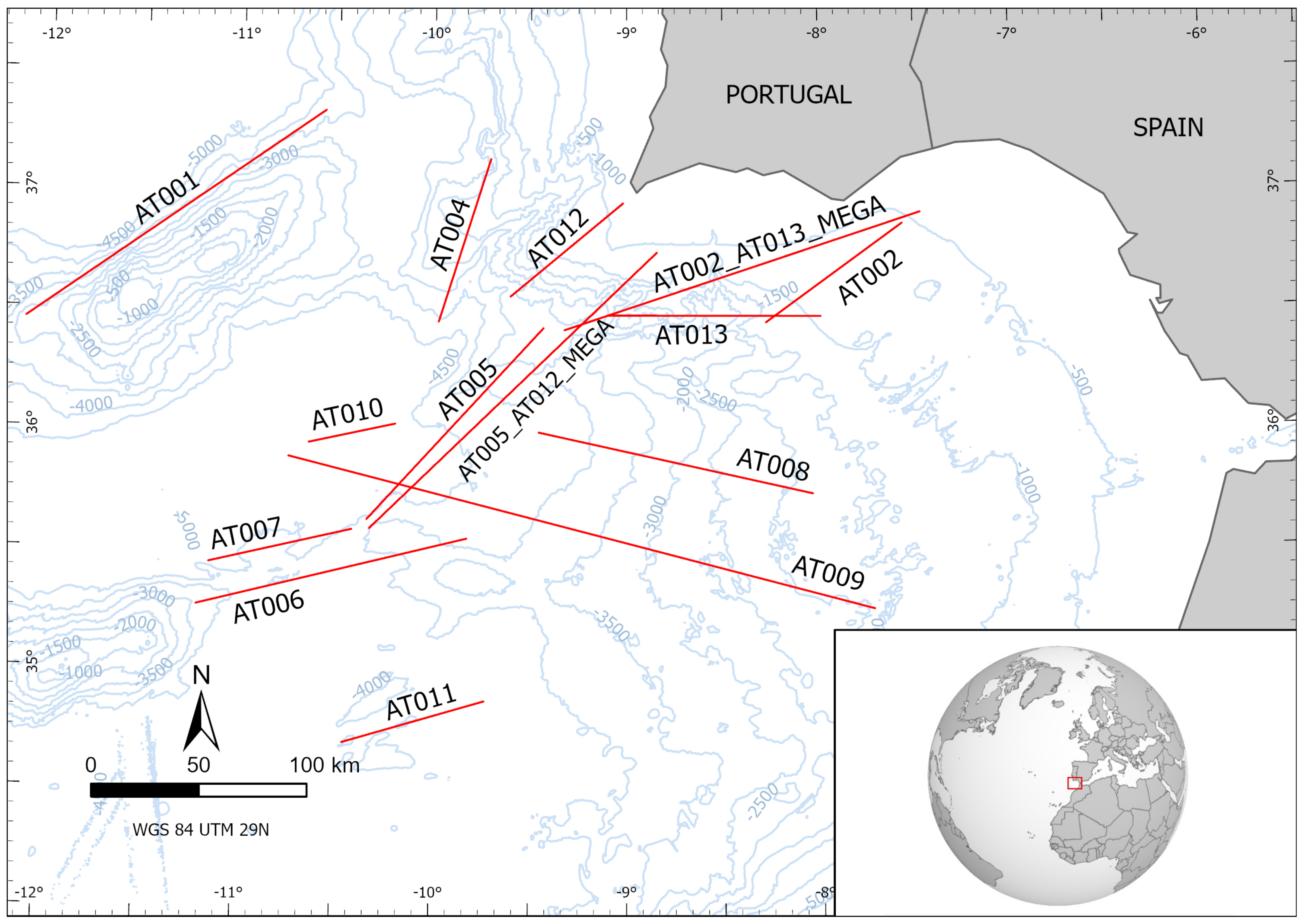
28], among others. A total of 12 faults were selected to be used in this study (
Figure 2) after careful review and update of available published information and considering the opinion of a number of experts gathered in a workshop devoted to this task held in 2017 [
29]. All the faults considered have published evidence of Quaternary activity, although this activity is very likely but has not yet been definitely demonstrated in the case of the Gorringe Bank (AT001), Guadalquivir Bank (AT002) and Portimao Bank (AT013) faults. Importantly, the so-called Cádiz Wegde Thrust, which some authors assume still involves an ongoing subduction process, was discarded here as there is evidence of inactivity since upper Miocene times [
30]. Finally, two additional fault-sources were included to consider potential ruptures comprising two main faults, the Horseshoe and San Vicente (AT005 + AT012) and the Guadalquivir and Portimao (AT002 + AT013) (see
Section 3.1).
2.2. Topobathymetric Data Description
The elevation data used for the simulations in the studied area have different resolutions and origins. Concerning emerged terrain elevation data at 5 m pixel resolution, two options were readily available for the project. One option was the data published by the National Geographic Institute (IGN), covering the whole Spanish territory. It can be downloaded from the website [
31]. This data was obtained with LIDAR technology and was processed by IGN to derive diverse types of elevation model. The second option was the national Spanish elevation model generated by IGME using IGN’s original data, including LIDAR and other IGN archives (such as stereocorrelation photograms at 25 to 50 cm pixels). This elevation model was processed, in particular, to aid in the construction of the National Continuous Geological Map (GEODE), bearing in mind other geological needs. Both models excel in their quality and extent, and may be the best suited for different purposes. Some comparison work carried out between both elevation models indicated that the IGME processing results better represented the geometry of the topographical surface suitable for tsunami simulations since it further cleaned the data of different objects (such as greenhouses, buildings, trees or bridges). This is a critical feature when computing inundation since it prevents most (yet certainly not all) unreal barriers an inundation may face. It is important to note that the IGME model does not include the most up-to-date data from the IGN, as post-processing the entire country at 5 m pixel resolution using the most recent data takes quite a long time and much effort. Therefore, the IGME elevation model at 5 m pixel resolution derived from the IGN data was used, with a granted maximum error 90% lower than 1 m. It should also be noted that the IGME model may present some lower quality results in shadowed slopes than the IGN model because some of the input sources are stereo-imaging in nature—even so, it is more suitable for the purposes of this study but may not be adequate for other approaches or studies.
Regarding submerged topography information (bathymetry), the readily available data comes from different providers at different resolutions and have been obtained by different methods. On the one hand, shallow bathymetry used for the Huelva coast has 20 m pixel resolution, as provided by the Andalusian Environmental Information Network (REDIAM). On the other hand, bathymetric data selected for simulations in the Cádiz region is at 5 m pixel resolution, as provided by the former Ministry of Agriculture, Fisheries and Food (MAPAMA), now the Ministry for Ecological Transition and Demographic Challenge (MITECO). Taking into account that these high-resolution data do not cover the entire region of interest of the project, other sources of information have been used to account for open sea areas and, therefore, to simulate wave propagation. For those regions without high-resolution data, models from the European Marine Observation and Data Network (EMODnet) and The General Bathymetric Chart of the Oceans (GEBCO) at 1/16 arc-minutes (≈115 m) and 15 arc-seconds (≈450 m) pixel resolution, respectively, were used. Both databases are freely available at their respective websites [
32,
33].
2.3. Pseudo-Probabilistic Approach. Random Variables Distribution and Sobol Sampling Method
Models to simulate tsunamis triggered by seismic events require, in the first instance, to reproduce the initial displacement of the water-free surface produced by the transfer of energy from the movement of the seafloor as a consequence of the fault rupture. As mentioned previously, most commonly accepted and used solutions for co-seismic seabed displacement follow Okada’s work [
34], which is presented in a relatively simple and analytic form. Then, the static seafloor deformation is directly transmitted to the free surface as an initial condition [
35]. Due to the uncertainty related to the determination of the Okada parameters, the simulation of the 14 faults that have been considered for the present study, may be insufficient if the goal is to understand the economic impact that any potential seismic tsunamigenic source of a given probability could produce. Accounting for a given probability is a requirement derived from the EU regulations on insurance after the Solvency II Directive 2009/138/EC. Hence a deterministic approach to unraveling a random problem in nature may not be the best approach to take. An alternative is to account for uncertainty in some of the parameters involved in the seafloor deformation. This idea is the basis of a pseudo-probabilistic study of economic impact. An artificial seismic register is generated by means of the uncertainty associated with some Okada parameters, then each artificial event is simulated and used for the economic impact assessment.
The best case scenario for a pseudo-probabilistic approach would be to consider uncertainty for all the Okada parameters, to the extent that many more different scenarios would be taken into account. However, appropriately exploring a 10-dimensional continuous parameter space for each fault, and consequently simulating every crafted event would implicate a computing power that is currently unattainable or unreasonable costly. If all ten Okada parameters were to be sampled only three times, for both extremes and the average, the amount of combinations to produce an adequate coverage of the input parameter space would increase to , which in turn would boost the simulation needs beyond combinations. Moreover, sampling only the extreme values and the average may not appropriately describe the spectrum of damage, considering the highly non-linear issues involved that play a major role. These include wave propagation, wave interaction with the coast and the bathymetry, the elevation data, inundation, and, last but not least, the distribution of elements subject to damage.
As the fault-source modeling employed for this investigation assumes geometric values for which maximum seismic rupture is plausible, parameters, such as dip angle, fault length and width, remain fixed as they illustrate maximum potential values. Furthermore, all faults are assumed to be composed by a single segment. Although variations in segmentation number can have a major impact on inundation results, their assessment would imply adding an Okada parameters list for each segment, thus exponentially increasing the number of possibilities to be combined for a single fault. With respect to the remaining parameters, some tests have been carried out to assess which of them may be described as the driving factors. It is clear that some parameters involve more uncertainty than others, such as strike, rake and slip. For example, although the strike parameter is fairly well-known, it measures fault orientation with respect to the north; thus, minor variations of this orientation could lead to situations where completely different areas become flooded. On the other hand, the rake parameter is chosen to vary to reflect its natural variation along the fault depending on the deflections of the strike with respect to the stress field. Therefore, slip as a random variable is assumed to follow a Gaussian distribution, whilst strike- and rake-associated random variables, due to their circular nature, are considered to follow a Von-Mises distribution.
To reduce the number of scenarios to be simulated, and considering that the resulting economic damage distribution is unknown, such distributions require to be sampled.
In relation to random variable sampling methods, there are several sampling techniques [
36], including random-sampling, stratified sampling, Latin hypercube sampling (LHS) and quasi-random sampling with low-discrepancy sequences. Random sampling means that every case of the population has an equal probability of inclusion in the sample. It is a very straightforward method; however, it can lead to a set of gaps or clustering, meaning that there would be some sampled areas overemphasised and some non-sampled areas. Stratified sampling tackles the problem of dividing the input space into strata (or subgroups) and a random sample is taken from each subgroup. This has the advantage of obtaining representation from all the space, although some gaps may still appear. LHS is a type of stratified sampling where each parameter is individually stratified over
levels, such that each level contains the same number of points ([
36], p. 76). It can have the advantage of requiring less samples to adequately describe the input space, but this depends on the function to be sampled [
37]. Quasi-random sampling sequences are designed to generate samples as uniformly as possible over the unit hypercube. Unlike random numbers, quasi-random points know about the position of previously sampled points, avoiding the appearance of gaps and clusters. One of the best known quasi-random sequences is the Sobol sequences.
The main sampling techniques have been tested in the context of building simulation by MacDonald and Burhenne et al. [
37,
38], which indicated that the Sobol sequences were superior to LHS, stratified sampling and random sampling in terms of mean convergence speed. In addition, the Sobol sequences method reduced the variability in the cumulative density function, which meant that it was the most robust method among those considered. Burhenne’s conclusions were that the Sobol sampling method should be used for building simulation, as the high computational cost requirements for the model make it impossible to run a large number of fully fledged simulations in a reasonable time. It is worth mentioning that the Sobol sequences have already been used successfully in the context of uncertainty quantification of landslide-generated waves [
39].
Bearing in mind that the work presented in this paper requires huge computational effort, and in light of the literature reviewed, the Sobol sequences were used as the sampling method to explore the input parametric space considered.
2.4. Simulation Software Tsunami-Hysea and Hpc Resources
The equations most widely accepted by the scientific community to model tsunami wave propagation in the open sea are the nonlinear shallow water equations (NLSWE) [
40]. This system of equations comes from a simplification of the Navier–Stokes equations for incompressible and homogeneous fluids, where vertical dynamics can be neglected in comparison to horizontal dynamics, and are set in the framework of a system of hyperbolic partial differential equations.
Nonetheless, NLSWE presents a downside when it comes to model inundation dynamics, since a tsunami wave arriving onshore generates a turbulent regime. Interaction with structures and sediments from the sea deposited on land makes 3D models a necessary tool to accurately simulate these turbulent flow dynamics [
41]. In spite of the availability of numerous effective 3D models, they are computationally expensive, rendering it impossible to run complex simulations in a reasonable time or at reasonable cost. Efforts focused on calculating acceleration have included techniques such as adaptative mesh refinement (AMR) [
42,
43] or multicore parallel computing [
44,
45]. However, in the last decade, a great paradigm shift occurred in terms of calculation units, with numerical methods traditionally implemented in CPU beginning to be implemented in a graphics processing unit (GPU) environment [
46,
47,
48], obtaining numerical simulations up to 60 times faster for real events [
49].
In this study, the required tsunami simulations were performed using the Tsunami-HySEA code. Tsunami-HySEA is a numerical propagation and inundation model focused on tsunamis that was developed by the EDANYA group at Málaga University in Spain. It implements most advanced finite volume methods, combining robustness, reliability and precision on a single model based on GPU structure, allowing simulation faster than real time. Tsunami-HySEA has been widely tested [
50,
51,
52,
53,
54] and has also been validated and verified following the standards of the National Tsunami Hazard and Mitigation Program (NTHMP) of the US [
55,
56,
57]. One key feature implemented in this numerical model is the possibility of using two-way nested meshing for high-resolution simulations. The nested mesh system approach allows computing of open ocean and offshore wave propagation using meshes of lower pixel resolution since the wave length is so long that the minimum number of points needed to adequately capture its form can extend to several kilometres. Near the coast, however, the wavelength is sufficiently small that higher pixel resolution meshes are used, both to reproduce its shape and to capture complex inundation features.
The simulation setup is described as follows. First, the Okada parameters are provided for every scenario. An open boundary condition is assumed on water boundaries, the Manning coefficient is set to 0.03, which is considered a good average value for natural bed roughness, the simulation time is set to 4 h, and the output variables are maximum water height, maximum velocity and maximum mass flow. Each simulation consist of a four-level nested mesh configuration that will be detailed in the next section.
To launch all the simulations, large computational resources are required. Today, high-performance computing (HPC) centers exist all over the world and provide HPC resources for scientific applications, which can be requested and accessed by researchers. These simulations were launched in the Barcelona Supercomputing Center (BSC) cluster, located in Barcelona (Spain). The specifications of this cluster are as follows:
Linux Operating System and an Infiniband interconnection network.
2 login node and 52 compute nodes, each of them:
- -
2 × IBM Power9 8335-GTH @ 2.4 GHz (3.0 GHz on turbo, 20 cores and 4 threads/core, total 160 threads per node)
- -
512 GB of main memory distributed in 16 dimms × 32 GB @ 2666 MHz
- -
2 × SSD 1.9 TB as local storage
- -
2 × 3.2 TB NVME
- -
4 × GPU NVIDIA V100 (Volta) with 16 GB HBM2
- -
Single Port Mellanox EDR
- -
GPFS via one fiber link 10 GBit
Each simulation was computed on a single GPU.
3. Results
In this section, a description of the numerical results obtained in the present study is provided. First, the complete set of the seismic sources used for the simulations is given. Then, the nested mesh configuration used for the numerical simulations is described. Later, the assignment of probabilistic distributions and the Sobol sampling process are described. Finally, this section concludes with a description of the numerical results that have been obtained.
3.1. Faults List
Figure 2 shows the distribution of the tsunamigenic fault-sources considered in this study and described in
Section 2.1. They correspond to complex faults compiled in the QAFI database but are modeled here as rectangular shapes from their basic geometric parameters: length, width, dip and strike (
Table 1). The slip was determined from the seismic moment equation [
58] considering the rupture area of the fault from the length and width, and a shear modulus that varies between 30, 40 and 60 GPa for faults in the continental crust, oceanic crust or exhumed mantle, respectively. The seismic moment was previously calculated from its relation with the moment magnitude according to Hanks and Kanamori [
59]. The moment magnitude was estimated from the empirical relationships recommended in Stirling et al. [
60].
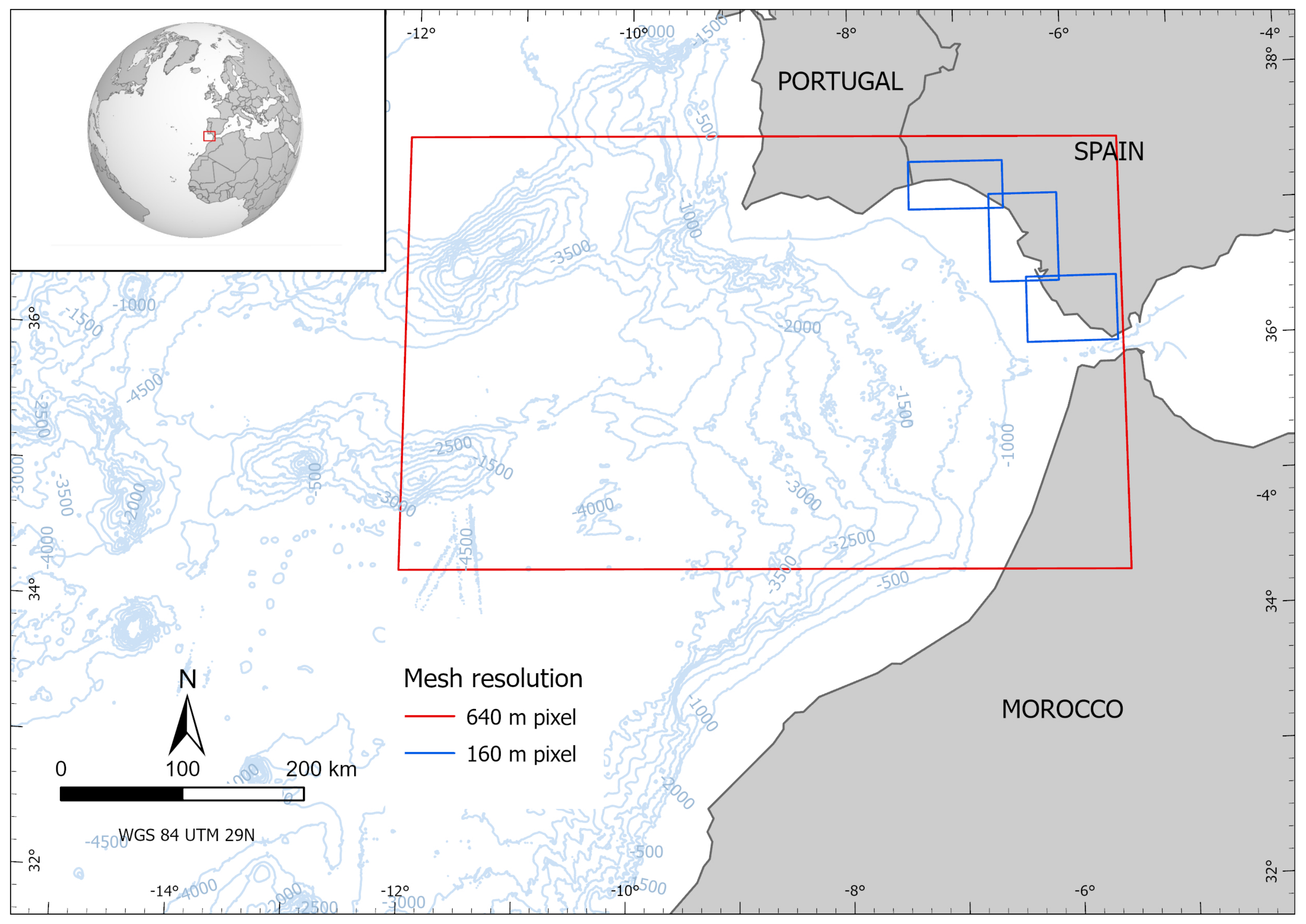
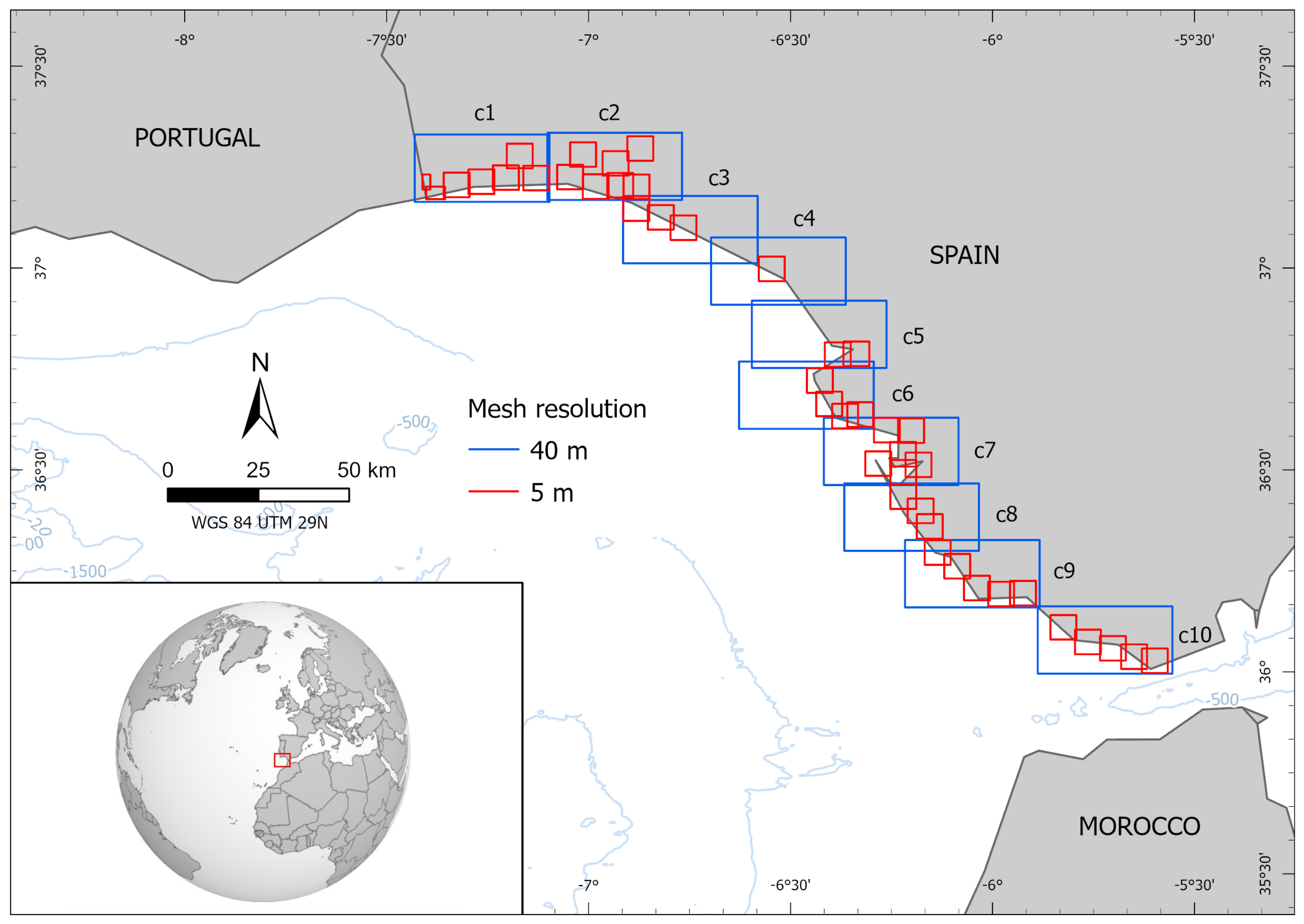
3.2. Nested Meshes Spatial Configuration and Resolutions
A set of four levels of nested meshes was considered to carry out the present inundation study at very high resolution along the Andalusian Atlantic coast. The computational domain is covered by the ambient mesh with a numerical resolution of 640 m per pixel, spanning from 34.28° N to 37.49° N and from 12.05° W to 5.5° W. Next, three levels of grids were nested, considering 3 meshes of 160 m pixel resolution, 10 meshes of 40 m pixel resolution and 43 meshes of 5 m pixel resolution that finally shaped the coverage of all areas of interest at high resolution.
Figure 3 and
Figure 4 show spatial configuration of the meshes. The areas not covered by the highest resolution meshes did not contain sufficient elements of interest for the purposes of this study, but should be included in future revisions if further urbanisation were to be undertaken.
Each 5 m pixel resolution mesh covers an area of 37 km, and each 40 m pixel resolution mesh covers an area of 515 km. The number of control volumes are the following:
Each 5 m pixel resolution mesh: 1,381,952 volumes.
Each 40 m pixel resolution mesh: 304,192 volumes.
Upper 160 m pixel resolution mesh: 104,448 volumes.
Middle 160 m pixel resolution mesh: 142,848 volumes.
Bottom 160 m pixel resolution mesh: 138,592 volumes.
640 m pixel resolution mesh: 470,400 volumes.
The total size of the computational problem to be solved for every single simulation, if they were performed as a single simulation, is quite large, composed of 63,322,144 volumes.
3.3. Assigning Probabilistic Distributions and the Sobol Sampling Process
As previously mentioned, the strike and rake parameters are assumed to follow a Von-Mises distribution, while the slip parameter follows a normal distribution. Given the fact that the available processed data that provide information on the uncertainty of these three parameters is only related to the mean () and the standard deviation (), some intermediate work is necessary to adequately describe each fault’s Von-Mises parameters. The process is represented as follows.
Recall that the Von-Mises (VM) distribution of the mean
and the dispersion
, denoted as
, has similar properties to the linear normal distribution. To estimate the Von-Mise distribution parameters of a circular random variable using mean and standard deviation sample values, conversion to radian units is first necessary. On the one hand, the mean value of the sample is used for the VM distribution straightforwardly. On the other hand, the standard deviation requires a different treatment, since it has to be adapted to the VM dispersion parameter,
. Under certain conditions, the parameter
can be considered as the inverse of the variance,
[
61]. The way to relate
with
has to do with the first trigonometric moment of the VM distribution [
62]. First define the quantity
(related to dispersion of circular random variable) and then solve
where
is the modified Bessel function of the first kind and
p the order evaluated in
. The Equation (
1) can be approximated using the maximum likelihood estimate
of
, which yields a piecewise function of
(see [
63], pp.85–86) defined as
This procedure allows establishing of the well-defined Von-Mises probabilistic distribution for the strike and rake parameters.
Table 2 shows the different probabilistic distributions assigned by applying the described procedure.
Once the probabilistic distributions have been constructed, the procedure used to sample the three-dimensional input space of each fault using the Sobol sequence technique is described below.
- 1.
Select a fixed number of samples N. The number of samples should be a power of 2 due to properties of the Sobol sequences, i.e., , . We choose .
- 2.
Generate a Sobol sequence of size N in three-dimensional unit cube. This will return a three-dimensional sequence with coordinates , each one inside the interval .
- 3.
Each coordinate
is used to sample the corresponding parameter, i.e.,
for strike,
for rake and
for slip. The way to obtain the sample is through the use of the inverse transform sampling method (see [
64], p. 28).
- 4.
Now that each coordinate is associated with its corresponding sample , the tuple (, , ) is chosen for the simulation.
The
Appendix A includes five tables detailing the sampled values using this procedure according to the probabilistic distributions specified in
Table 2. Extracting 64 samples expresses that each fault has 64 associated variations, adding a total of
synthetically generated events.
3.4. Numerical Simulations
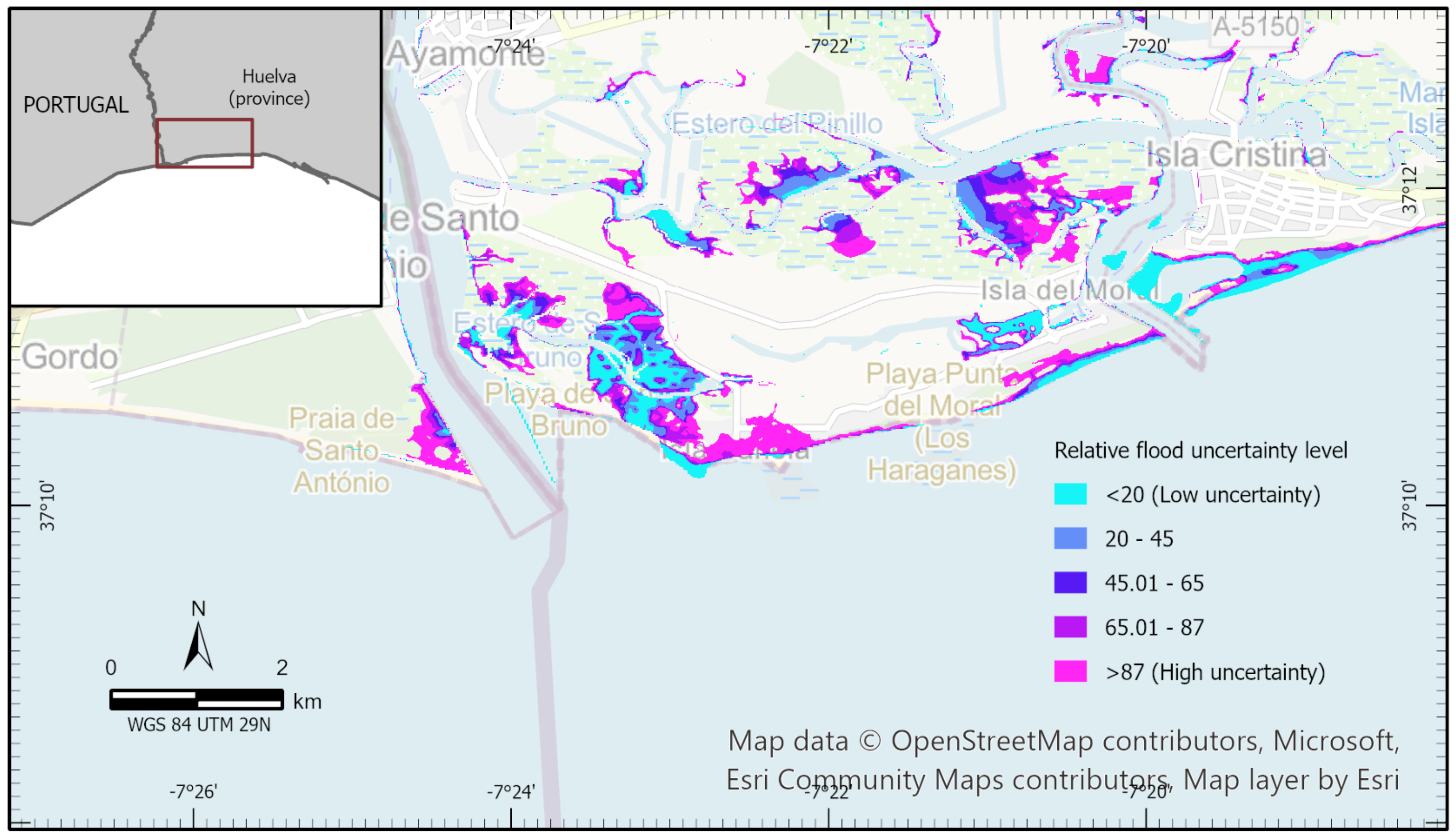
A total of 896 simulations were launched in the BSC cluster. The simulation runtime was around 4 h for each simulation. As mentioned before, the simulation outputs were maximum water height, maximum velocity and maximum mass flow at each 5 m resolution pixel, producing a 30 MB NetCDF file each. A total amount of 1.1 TB data was generated. Among the data contained in the entire constructed database, some results have been processed and represented to demonstrate how uncertainty in the fault-source parameters affects flood distribution. The illustrations depicted come from simulations of faults AT002 and AT013, as their epicenter locations are closer to the western coast of Andalusian. In order to exemplify the uncertainty in flood distribution, considering the uncertainty associated with the 64 variants of these faults, maximum water height data were prepared for two of the 40 m sub-grids, namely, c1 and c7. The inspection consists of counting how many times each land-located pixel of the 5 m grids contained within the 40 m grids has been wet, in consideration of the 64 fault variants. Each pixel counting is then transformed into relative flood uncertainty levels by application of the Weibull-like function
where
i accounts for the number of times the pixel has been wet and
n is the number of fault variants (
).
Figure 5 and
Figure 6 show the results obtained.
Figure 5 displays the relative flood uncertainty behaviour with respect to the 64 variants of fault AT013 inside the 40 m grid termed as c1. It is remarkable how the areas surrounding the diverse rivers are prone to be flooded, with flood uncertainty increasing as we move away from the river courses, in contrast to the poor penetration found through
Playa de Bruno and
Playa Punta del Moral, which display high levels of uncertainty. Although that is not the case for the beach on the far right side region.
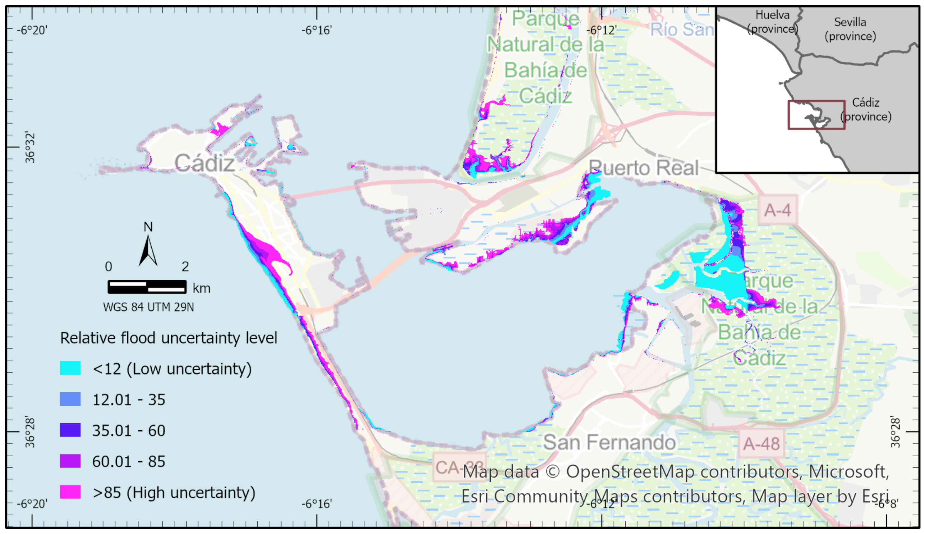
Moving on to the other area,
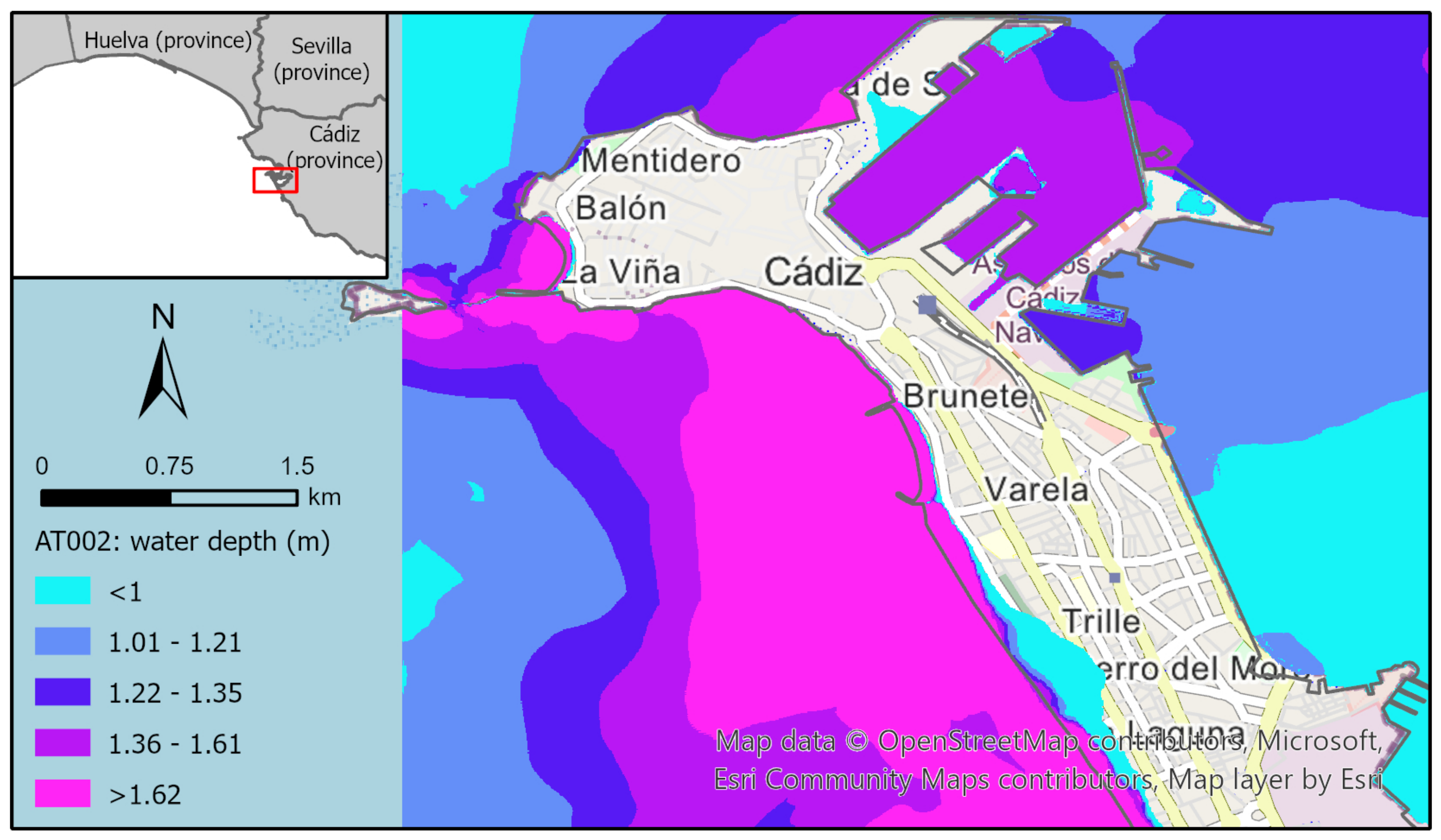
Figure 6 shows the relative behavior of the flood uncertainty with respect to the 64 variants of the AT002 fault within the 40 m grid termed as c7. It is still remarkable how flooding affects the river course’s surroundings, with low levels of uncertainty mainly found at the eastern rivers in
Parque Natural de la Bahía de Cádiz. However, greater flood penetration can be seen along the coast, particularly along the western side of the city of Cádiz and in the bay coast adjacent to
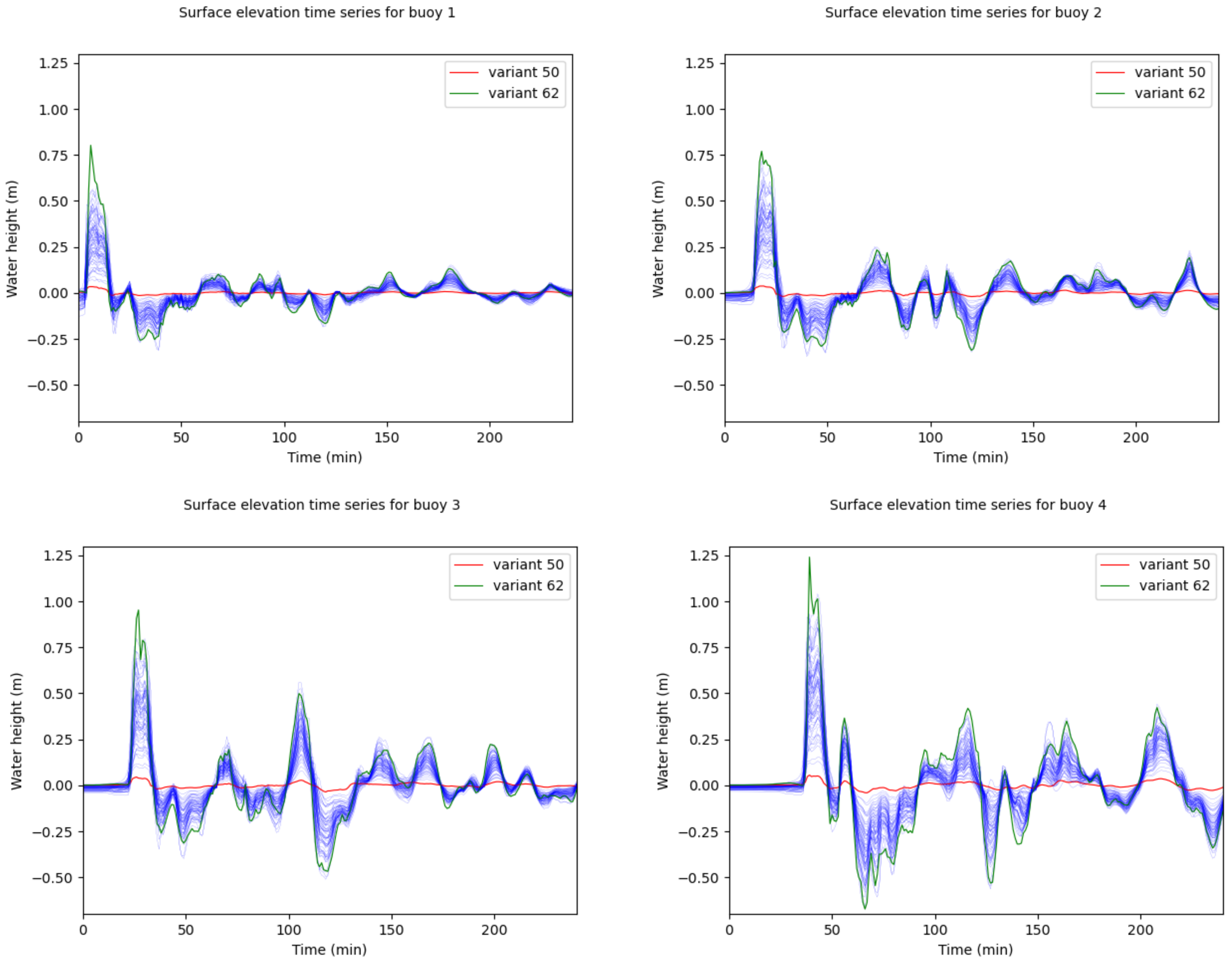
Puerto Real, where higher flood uncertainty is expected across some sections. In particular, the high-uncertainty area along the western coast of the city of Cádiz and the isthmus is mainly driven by variant 62, as is shown in
Appendix B. Both figures illustrate regions with low and high relative flood uncertainty. Low-uncertainty regions (blue) can be interpreted as being more independent of the uncertainty in the fault-source parameters, whereas high-uncertainty regions (violet) only get flooded under a very specific configuration in the source or by concrete sources.
In addition to the flood-uncertainty figures, some results concerning the maximum water depth, maximum current velocity and maximum mass flow are presented. These results were compiled to fully harness the computational resources reserved for the project at the BSC cluster, and keeping in mind their usefulness for future research. Nonetheless, the data regarding the maximum current velocity and maximum mass flow are not of particular interest for the purpose of the final product, since the estimate of the economic damage will be performed using the data of the maximum water height. Furthermore, isolated results such as these do not contain enough useful information to derive any compelling conclusion; it is necessary to look at all the simulation results to fully understand the underlying phenomena.
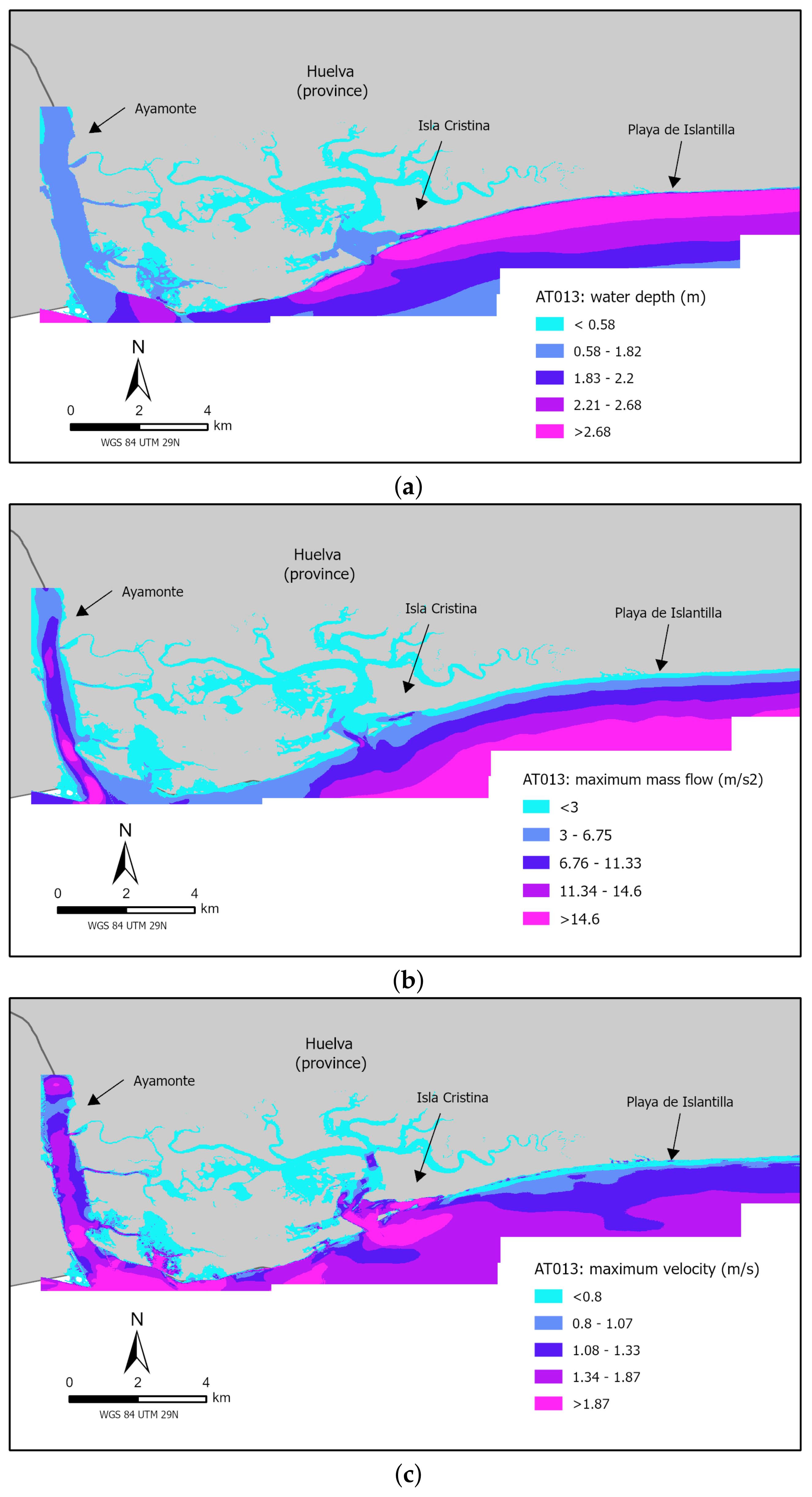
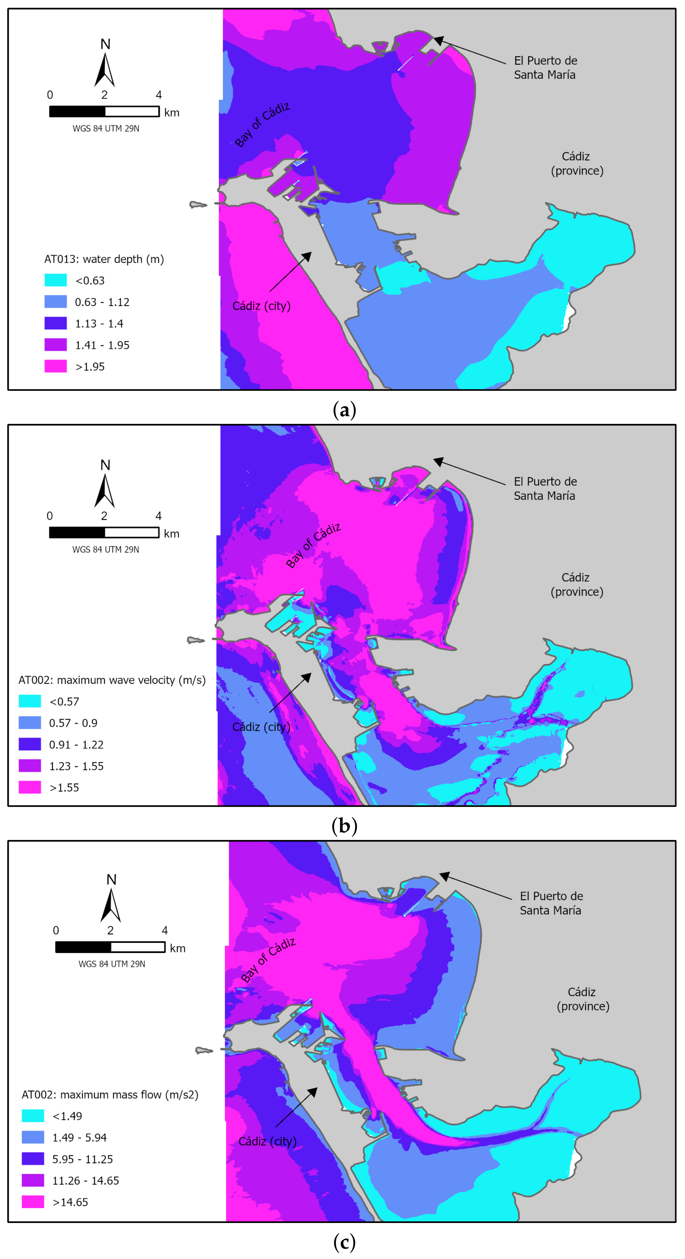
Next, the same faults and regions as before are considered, i.e., faults AT002 and AT013, but now we focus on the results concerning variant 37. Variant 37 was chosen because it presents the maximum slip value sampled for both faults.
Figure 7 shows three maps including the aforementioned output variables in the 5 m sub-grids placed inside the c1 grid.
Figure 8 displays similar data describing the results for the 5 m sub-grids placed inside the c7 grid. Both sets of figures show a slight land inundation. This is an excellent example of why the moment magnitude (related to the slip-rate value) is not the only active factor in terms of a widening in the flooded area, since, for example, variant 62 has a lower slip value but the inundated area is larger (see
Appendix B). Although the results presented in this section only account for data collected on some of the 5 m grids, they provide some insight into how uncertainty in the fault-source parameters affects wave propagation. This examination has been undertaken and pointed out in
Appendix B.
4. Discussion
The most recent advances in the field of tsunami hazard assessment research have been progressively oriented towards two main areas of study: scenario-based tsunami hazard analysis (STHA) and probabilistic tsunami hazard analysis (PTHA). One technique or the other is used depending on whether the objective of a project is to design evacuation plans, including evacuation routes, or to analyze various consequences related to damage. Regarding this topic, most of the literature is populated by STHA methods, which take advantage of few simulations to address the consequences of what is generally called “the worst case scenario”—namely, a theoretical unlikely devastating event. The focal point of some of these studies is reproducing past events from historical records for which inundation maps are generated based on intensity measures, such as water heights or run-up [
11,
13,
65,
66,
67]. In contrast to STHA, PTHA is a relatively new area of tsunami hazard research. Its foundations were formally established in 2006 with the pioneering work of Geist and Parsons [
68], which was grounded in a probabilistic seismic hazard analysis approach. The need to consider the uncertainties involved in seismic-triggered tsunami events, together with the enhancement in computing power, has steadily led to establishing PTHA as the standard viewpoint in this matter [
14,
15,
16,
17,
18,
19,
68,
69,
70]. This novel vision in dealing with problems of this nature is founded on the motivation to account for part of the inherent uncertainty in the entire generation-propagation-inundation process of a tsunami event. The key idea in the procedure is to avoid the limitations derived from considering a small set of potential catastrophes, and to produce a catalogue of varied events with the intention of reaching some conclusions in light of all the possible scenarios. The primary results deriving from these investigations are generally directed at risks, commonly related to insurance, or stochastic inundations maps. Moreover, by virtue of assigning fixed return periods to the phenomena (normally seismic ones), probability exceedance maps can be derived, in which the water height or current velocities information delivered is linked to the occurrence probabilities. In this study, we provide a major insight into why the deterministic reference frameworks mentioned above may fail to adequately identify the worst case scenario, since the non-linearity of all elements may lead to the worst consequences far from the largest seismic occurrence. A probabilistic view is difficult, but it is attainable today, and should be the way forward. The methodology followed throughout our work could be placed intermediately between STHA and PTHA. We have shown how to design a synthetic inventory of tsunamigenic events without explicitly prescribing return periods to them. Although we have not produced results comparable with other PTHA studies, what is comparable is the process of building the synthetic inventory. A common way to reconstruct this database consists of fixing some of the Okada parameters and using any sampling strategy to obtain the remaining parameters. Another methodology commonly found in the literature considers randomly distributed heterogeneous slip models [
15,
70], where several variants of an archetypal slip model are linked to a single fault in a process where the fault is divided into multiple subfaults and a random-generated slip is designated to each one of them. Then, the co-seismic seafloor deformation is calculated empirically from the slip and spatial distribution of the constructed subfaults, providing the initial water elevation by a simple one-on-one translation. This alternative practice for generating the database is a powerful tool when the activity is focused on the underlying uncertainties across complex fault rupture mechanisms. In the context of the previous way of building the database just described, some authors (such as González et al. [
16] and Zamora et al. [
69]) have designed probable seismic ruptures aiming to cover a wide variety of moment magnitude values. In [
16], parameters such as strike, rake and dip remain fixed, while the main effort is concentrated on sampling a seismic moment cumulative density function and thereafter generating slip and fault area size values using some empirical relations. In [
69], the authors adopt Gutenberg–Richter’s law to estimate b-values, annual earthquake rate and maximum moment magnitude with the purpose of sampling events that incorporate a significant range of seismic moments with respect to predetermined exceedance probabilities. Additionally, they use uniform and normal distributions, as well as empirical relationships to estimate the rest of the geometric parameters. In [
71], the artificially crafted register is undertaken via a movement along the fault trace of what the authors termed a typical fault, which is a fault with pre-established Okada parameters in a determined source zone. The González et al., and Zamora et al., approximations have the advantage of generating events that cover a wide spectrum of seismic magnitude, thus indirectly taking into account a large limit of slip values (according to the seismic moment scalar equation [
58]). We are aware that either increasing seismic moment or slip values can lead to amplification in the run-up, thus widening the flooded section. Our perspective adds uncertainty directly to the slip variable, without examining the seismic moment directly. Furthermore, we also acknowledge that the moment magnitude or slip rate are not the only variables that play an important role in understanding flood distribution, in as much as the fault segmentation number or the fault-plane dimensions may strongly contribute to it. As mentioned in
Section 2.3, this work is based on fault models with the number of segments set to 1, while the fault-plane dimensions and dip angle remain fixed as well. Therefore, in order to capture differences in fault orientation and strike deviations from the stress field, we have emphasized the variability in strike and rake parameters.
In addition to the treatment of uncertainty already mentioned, it is also worth noting the high-resolution simulations that have been carried out and on which this work is based, together with the large extension of the coast that has been covered. The final objective of this project is to examine all the Spanish coasts. In the literature, authors state that, depending on the territory of study and on the local authorities, the available elevation data may or may not be adequate for the final objectives of the project. In [
69], the authors use a single 1 arc-min resolution bathymetry to compute the propagation, and then, using some techniques such as Green’s Law, they project wave height at some offshore locations towards the coastline. They state that formulas such as Green’s Law are needed today because accurate modeling of the tsunami propagation and coastal impact over high-resolution nearshore bathymetry is not yet feasible for regional-scale PTHA, due to high computing resource requirements when targeting hundreds of thousands of seismic scenarios. Their concerns are justified as their inundation modeling is over 4000 km-long, making accurate data acquisition a major issue. Our study, however, is intended to grasp knowledge about inundation in a country-scale scenario and is committed to high-resolution grids in a pseudo-probabilistic scope, meaning that tens of thousands of simulations are being undertaken, covering a 2000 km-long coast. The numerical results presented here represent only a small part of the full picture we are elaborating. The aforementioned statement about infeasibility could derive from factors of limited time, limited computational resources, or even limited high-resolution elevation data collected; however, in general, we believe that, if suitable data are already available, in combination with sufficient HPC resources, the most recent tsunami codes are able to reproduce high-resolution inundation for country-scale dimensions in a matter of months. Even so, it is common knowledge that expensive computational resources for an accurate PTHA study are the main downside. Recent work aimed at circumventing this problem makes use of stochastic approximations, called emulators, built upon a pre-computed training set [
20,
21,
39]. An emulator can be seen as an interpolating operator of the map that assigns to each input parametric array its corresponding desired output through a fully fledged simulation. The emulator encompasses the whole generation, propagation and inundation process without explicitly computing, thus allowing output predictions and uncertainty quantification at fairly low computational cost. The effectiveness of an emulator approach is closely related to the construction of the training set, which is its core. In [
20], the epicenter location and moment magnitude were sampled using the LHS method to simulate 300 scenarios and retrieve the maximum water height and maximum current velocity at several locations, which in turn constitute the basis for building the training set. In [
21], the authors sampled a seven-dimensional input space using a sequential design MICE algorithm to generate a training set of 60 simulated scenarios. Their sampling technique outperforms the LHS method in the sense that one-shot random sampling for the training set lacks the information acquisition achieved by the sequential design. One-shot methods, such as LHS, can overemphasize unnecessary regions and consequently waste computational resources. On the other hand, the sequential design takes into account the previously computed quantities to select the next input parameters for the next simulation batch.
Finally, recalling the grid resolution, other studies found in the literature reach highest resolution grid pixel sizes of 5 m, 10 m, 50 m, 52 m, 90 m, 93 m [
8,
9,
10,
11,
12,
13,
15,
16,
17,
18]. Probabilistic-oriented studies, such as [
14,
15], run many simulations, but either use a relatively coarse mesh (50 m and 500 m, resp.) or the affected area is relatively small, such as the studies centered only on Tohoku Island. An exception to these studies is the aforementioned emulator-oriented approach [
20,
21], where the highest resolution grid pixel sizes are 10 m and 30 m, respectively.
5. Conclusions
The methodology adopted in this study follows the general first-step framework in a PTHA environment, where a synthetic seismic catalogue is required to proceed with the subsequent examination. Furthermore, this study could be fully encompassed in the PTHA field if return periods and a logic-tree were added. Even without the probabilistic treatment arising from a potential attachment of return periods, the numerically computed database derived in this study regarding wave height, maximum velocity and maximum mass flow provides an excellent starting point to assess different tsunami-hazard-related issues, such as designing vulnerability functions, developing loss functions or evaluating structural losses (e.g., [
8,
9,
10,
14]).
In particular, our objectives are aimed at drawing conclusions about the economic-related damage distribution caused by a theoretical but plausible tsunamigenic event. In practice, we will determine economic damage due to a specific variation of a single fault in a specific region by overlaying the maximum water height data with the building-scale data in the insurance field. Based on the maximum height of the water column recorded on a single pixel containing any type of construction, an economic value will be associated with it due to a preselected vulnerability function. Adding together the pixel-scale damage estimates for all covered locations will deliver a mapping that links every fault variation to a singular value representing its potential economic damage. By repeating the indicated procedure for the variations of each fault, a probabilistic distribution of the economic damage will be naturally generated, which will be further analyzed. The damage distribution function may have little to do with the largest triggered magnitudes, or the damage may even not be concentrated around the largest flood-likely areas. Direct damage is only possible with the coalescence of any sort of valuable elements (such as people, property, services) with the consequent impact of the phenomena. Such direct damage may then be responsible for further indirect losses (due to the topological and dependent construction of human societies). Considering that neither valuable items nor the value itself are uniformly distributed, in addition to the fact that what is insured, and up to how much, is also unevenly allocated, a probabilistic approach makes more sense to better understand the final damage curve distribution. The most likely damage estimation in terms of monetary loss for the insurance sector cannot be evaluated without considering the full extent of uncertainties in the source and their effects in flooding valuable assets. The results of this work show that some areas are less influenced by the uncertainty in the triggering mechanisms, whereas other areas will only get flooded under a very specific set of triggering conditions. If we only account for one of those sets (a scenario-based approach), it is unclear whether the resulting damage belongs to the most likely output of the many uncertain initial conditions or is actually a representative event of the outcome considering variations in the initial conditions. This method contributes to a better understanding of the damage function, providing crucial and non-pre-existing information for the insurance sector to make better-informed decisions.
Concerning other applications, water height data can also be exploited to understand nearshore and onshore flood distribution from an arbitrary tsunami of Atlantic origin, facilitating the production of stochastic inundations maps and evacuation routes for people living near the coast. Additional information regarding maximum velocity and maximum mass flow can undoubtedly be useful in approaching the evaluation of particular structural damage.
We would like to highlight the importance of the results of this article concerning the numerous computed numerical simulations in conjunction with their high-resolution discretization, where each simulation has produced relevant information for the outstanding population nucleus placed alongside the Atlantic Andalusian coast in building-scale detail.
Future research with reference to this topic should aim to exploit the generated database in search of building-related information of interest in the field of PTHA. The extra work required to achieve these objectives would undeniably be worth the immense enhancement in people’s safety and tsunami risk management by regional and local authorities.


 ,
, 


