A Gaussian Model for the Time Development of the Sars-Cov-2 Corona Pandemic Disease. Predictions for Germany Made on 30 March 2020

Abstract

For Germany, it is predicted that the first wave of the corona pandemic disease reaches its maximum of new infections on 11 April 2020 $\stackrel{+5.4}{-3.4}$ days with 90% confidence. With a delay of about 7 days the maximum demand on breathing machines in hospitals occurs on 18 April 2020 $\stackrel{+5.4}{-3.4}$ days. The first pandemic wave ends in Germany end of May 2020. The predictions are based on the assumption of a Gaussian time evolution well justified by the central limit theorem of statistics. The width and the maximum time and thus the duration of this Gaussian distribution are determined from a statistical ${\chi }^2$-fit to the observed doubling times before 28 March 2020.

1. Introduction

In these days there is a very high interest in the societal, economical and political world to understand the time evolution of the first wave of infections of the population by the current Sars-Cov-2 (corona) virus. The most important issues are the total duration and the peak time of the infection evolution as well as the maximum number of daily infections. It would be most helpful for many people to have a reproducible, crude, but reliable estimate when this pandemic wave is over. It is the purpose of this manuscript to provide such an estimate based on a simplified Gaussian model for the time development of the pandemic outburst.

The best justification for the Gaussian, or normal, distribution for the virus time evolution is given by the central limit theorem of statistics [1]. The central limit theorem states that in situations, when many $(\gg 1)$ independent random variables are added, their properly normalized sum tends toward a Gaussian distribution even if the original variables themselves are not normally distributed. The spread of the virus infection of populations with high number of persons certainly is such a random process to which the central limit theorem is applicable. Each person in a given population has a probability distribution (normalized to unity) as a function of time of being infected: it is a very noncontinuous distribution being 1 at the day of infection and 0 on all other days. If one adds up these discrete distributions of persons living in villages and districts of towns of typical size of about 1000 persons one obtains quasi-continuous probability distributions for being infected which certainly will be different in hotspots of the disease and isolated rural areas. If we then add up a large number of these village probability distributions for all of Germany we obtain the daily infection rate distribution which according to the central limit is close to a Gaussian distribution. Recently, the Gaussian model has also been used to predict the time evolution of the COVID-19 pandemic in Italy [2] and China [3]. To the best of our knowledge this manuscript is the first application of the Gaussian model to the COVID-19 pandemic in Germany. It differs from the earlier work [2,3] by proposing the use of monitored doubling times to infer the total duration and the peak time of the first wave of infections.

The analysis of Gaussian distribution function plays a central role in many problems of statistical physics and plasma physics e.g., in plasma kinetic theory they are referred to as drift-Maxwellian [4] or counterstreaming bi-Maxwellian [5,6] velocity distribution functions.

Apart from consulting several reviews [7,8,9], as non-virologists we are not familiar with the recent relevant virology literature. Nevertheless, it is our hope that in these hard times an estimate by unbiased non-experts might be welcomed by specialists as well as the broad population, especially if some positive information and outlook is provided. We base our parameter estimates on publicly available information, especially by the podcast [10] and the recent sophisticated modeling study for Germany [9].

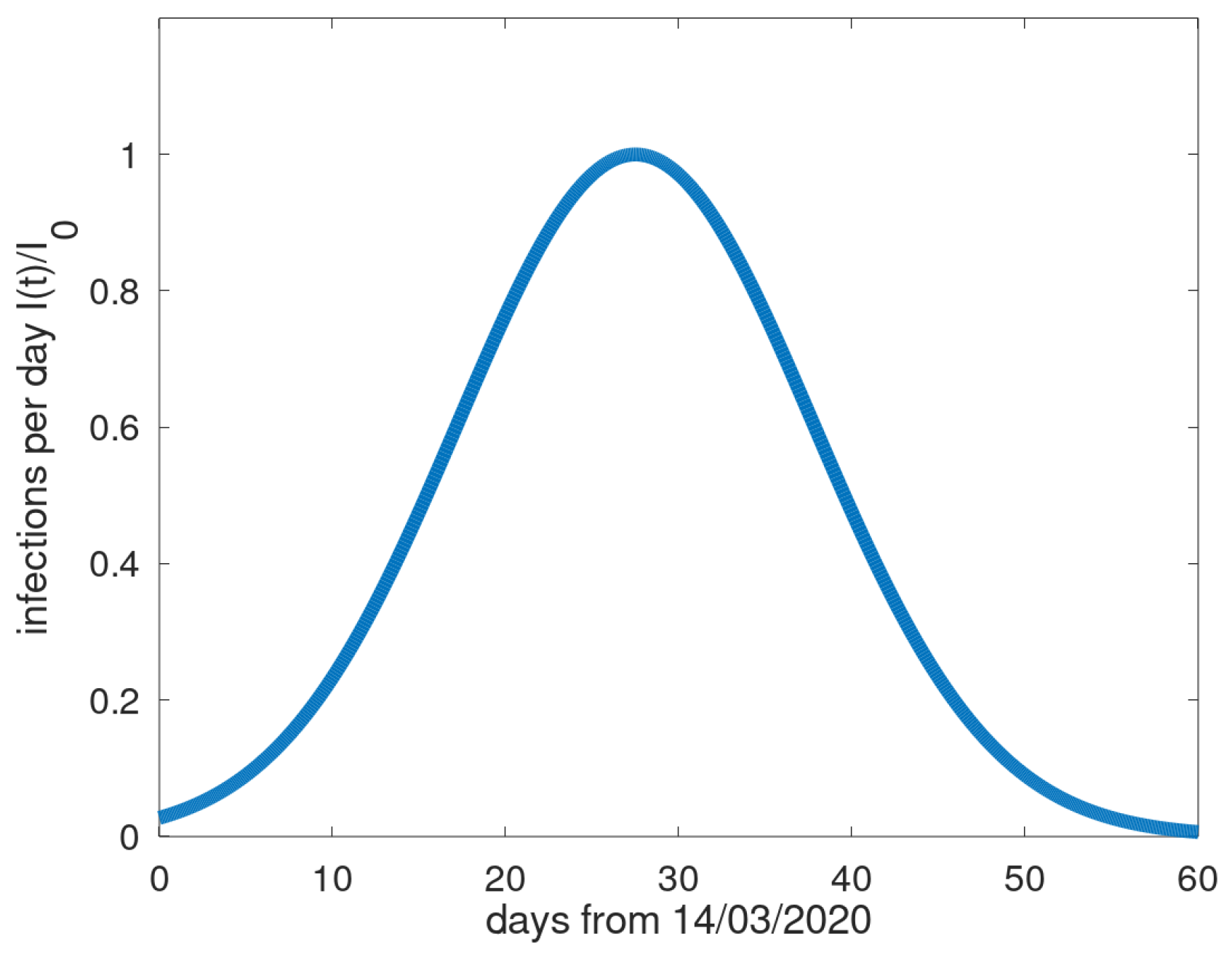
2. Gaussian Model

Numerical simulations and the empirical data of earlier epidemics [10] indicate that the time evolution of epidemic waves is characterized by an early exponential rise until a pronounced maximum is reached followed by a rapid decrease. As argued above, we adopt a simple Gaussian model for the time evolution of infections and explore its consequences. If $I\left(t\right)$ denotes the number of infections per day, we assume that its time evolution is given by the Gaussian function

$$I\left(t\right)=I_0{e}^{-{\left(\frac{t-E}{\Delta }\right)}^2},$$

(1)

shown in Figure 1, where $I_0$ denotes the maximum value at time E and $\Delta$ denotes the width of the Gaussian.

By monitoring the new daily infections, one easily derives the relative change in the infections per day

$$P\left(t\right)=\frac{dI\left(t\right)/dt}{I\left(t\right)}=\frac{dlnI\left(t\right)}{dt}=2\frac{E-t}{{\Delta }^2},$$

(2)

where we used the distribution Equation (1).

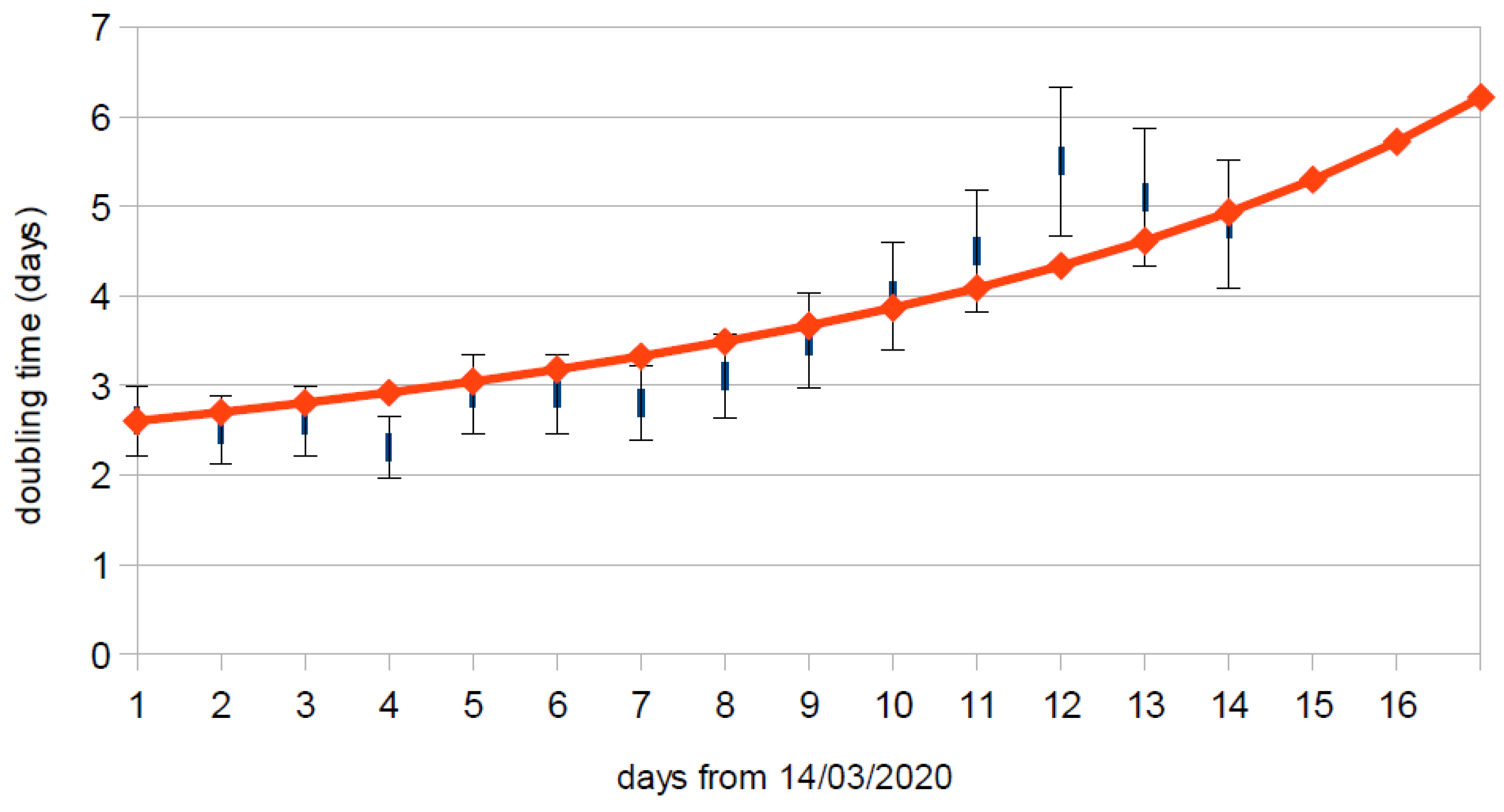
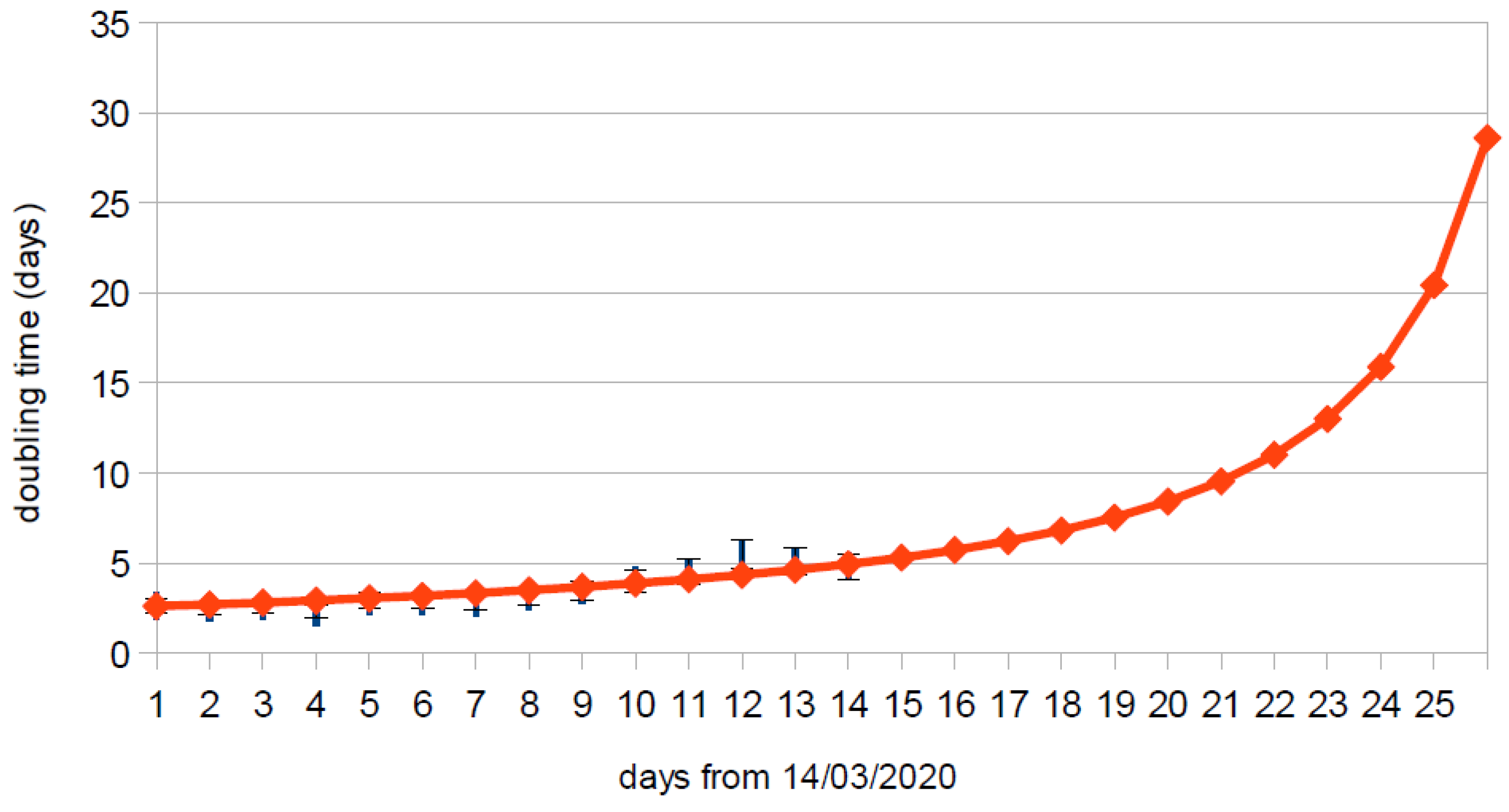
2.1. Doubling Time

The monitored data are often given in terms of the doubling time D of the corresponding exponential function at any time

$$I_a\left(t\right)=J_0{e}^{\frac{tln2}{D}}.$$

(3)

Using the distribution of Equation (3) in Equation (2) provides for the relative change in daily infection rate

$$P\left(t\right)=\frac{dln{I}_a\left(t\right)}{dt}=\frac{ln2}{D}.$$

(4)

Equating the two results in Equations (2) and (4) leads to the time-dependent Gaussian doubling time

$$D\left(t\right)=\frac{A}{E-t},A=(ln\sqrt{2}){\Delta }^2=0.35{\Delta }^2.$$

(5)

Figure 2 shows the monitored doubling times for Germany [11] starting from 15 March 2020 until 28 March 2020. We assume that every value has an error of 15%. It starts at $D(t=0)=2.6$ days and increases to $D(t=14)=4.8\pm 0.72$ days on 28 March 2020.

The Gaussian doubling time modeling then provides $D(t=0)=A/E=2.6$ days, corresponding to

$$\Delta =\sqrt{\frac{2.6E}{ln\sqrt{2}}}=\sqrt{7.5E}.$$

(6)

Moreover, Equation (5) reduces to

$$D(E,t)=\frac{2.6}{1-\frac{t}{E}}.$$

(7)

2.2. Statistical Fit

We determine the value of the only free parameter E in Equation (7) by performing a ${\chi }^2$-fit to the data shown in Figure 2. If $m\left(t_i\right)$ denote the observed doubling times at days $t_i$, $\delta m\left(t_i\right)=0.15m\left(t_i\right)$ its error and $D(E,t_i)$ the theoretical doubling time for given values of E, we calculate

$$\begin{array}{ll}{\chi }^2\left(E\right)& ={\displaystyle \sum _{i=0}^N}{\left(\frac{m\left(t_i\right)-D(E,t_i)}{\delta m\left(t_i\right)}\right)}^2\\ & ={\displaystyle \sum _{i=0}^N}{\left(\frac{m\left(t_i\right)-D(E,t_i)}{0.15m\left(t_i\right)}\right)}^2.\end{array}$$

(8)

Currently, on 28 March 2020 we have $N=14$ measurements. With one free parameter the number of degrees of freedom is $N-1=13$.

The best fit with the minimum value of ${\chi }_{\min }^2=9.51$ is provided for $E=27.5$ days. The ${\chi }_{\min ,\mathrm{p}.\mathrm{d}.\mathrm{f}}^2=9.51/13=0.73$ per degree of freedom (p.d.f.) is less than unity indicating that our model fits the data very well. For 90% confidence all values of ${\chi }^2\le {\chi }_{\min }^2+2.71=12.22$ are acceptable [12] yielding with 90% confidence that

$$E={27.5}_{-3.4}^{+5.4}\mathrm{days},$$

(9)

corresponding to 11 April 2020 $\stackrel{+5.4}{-3.4}$ days. Consequently, the best fit Gaussian doubling time for Germany is given by

$$D_{\mathrm{best}}=\frac{71.5}{27.5-t}\mathrm{days}.$$

(10)

As an aside we note that the variation in Equation (10) becomes infinitely large as $t\to 27.5$. Moreover, for times $t>E$ the doubling times becomes a decay half-life approaching 0 for very large times $t\gg E$.

Moreover, after inserting the values of Equation (9) into Equation (6) yields with 90% confidence

$$\Delta ={14.4}_{-1.0}^{+1.4}\mathrm{days}.$$

(11)

In Figure 3 we show the prediction of the doubling times in Germany until day 25 corresponding to 8 April 2020.

3. Predictions for Germany

3.1. Total Number of Infections

It is known that during the whole duration of the first wave of the virus evolution 70% of the total population are infected [10], if nothing is done to reduce the number of infections. Scaling the total population in units of ${10}^5{N}_5$ ($N_5=N/{10}^5$, where N denotes the number of persons), we estimate that $0.7q{10}^5{N}_5$ are infected during the whole duration of the first virus wave, where the quarantining factor q accounts for the currently taken political actions such as quarantining of elder and infected people, social distancing actions in the society as well as the closure of schools and daycare facilities.

Integrating the Gaussian in Equation (1) over all times we then obtain

$$7·{10}^{4}q{N}_5=I_0{\int }_{-\infty }^{\infty }dt{e}^{-{\left(\frac{t-E}{\Delta }\right)}^2}$$

$$=I_0\Delta {\int }_{-\infty }^{\infty }dx{e}^{-x^2}=\sqrt{\pi }{I}_0\Delta ,$$

(12)

where we used the integral ${\int }_{-\infty }^{\infty }dx{e}^{-x^2}=\sqrt{\pi }$. Equation (12) yields for the maximum value

$$I_0=\frac{7·{10}^{4}q{N}_5}{\sqrt{\pi }\Delta }=\frac{4·{10}^{4}q{N}_5}{\Delta }.$$

(13)

With the 90% confidence value for $\Delta$ from Equation (11) we obtain with the same confidence level for the maximum value in Equation (13)

$$I_0=\left({2.78}_{-0.22}^{+0.20}\right)·{10}^{3}q{N}_5.$$

(14)

3.2. Manageable Infections

We assume as typical medical parameters those suggested by the recent modeling by the Robert-Koch-Institute [9] (see their Figure 1): only about 20% of the infected people are seriously infected, 5% have to be hospitalized and $\alpha$% ($\alpha$ is often adopted to be unity) need access to breathing apparati for typically 1 week, corresponding to 7 days. We refer to the latter as NSSPs standing for new seriously sick persons per day. As these numbers are uncertain we keep their scalings with the typically adopted numbers.

In Germany there are at most 56,000 breathing apparati in total available, corresponding for a population of 80 million people to $70b_{70}$ (with $b_{70}=b/70$ where b is the number of breathing apparati) breathing apparati available per ${10}^5{N}_5$ people. As a consequence, every day the hospitals can handle $I_n$ NSSPs with

$$I_n=\frac{70b_{70}{N}_5}{7w}=10\frac{b_{70}{N}_5}{w}.$$

(15)

The infections are handable by hospitals for all times if at the maximum of the virus evolution $0.01\alpha I_0$, denoting the maximum number of seriously sick persons per day needing access to breathing apparati, is less or equal to $I_n$, i.e.,

$$0.01\alpha I_0\le 10\frac{b_{70}{N}_5}{w}.$$

(16)

Inserting the value of Equation (14) for the maximum value $I_0$, the quantity $N_5$ cancels out and we obtain with 90% confidence the condition

$$\left({2.78}_{-0.24}^{+0.20}\right)\alpha q\le \frac{b_{70}}{w},$$

(17)

which is equivalent to

$$\frac{\alpha qw}{b_{70}}\le {0.36}_{-0.03}^{+0.04}.$$

(18)

In order to handle all serious infections in German hospitals the condition in Equation (18) has to be fulfilled. It seems that German hospitals can only ensure the best treatment of all NSSPs at the maximum of the first wave if either (1) the number of available breathing apparati can be increased by a factor of 3, corresponding to $b=210$ per day, or (2) the quarantine factor q can be reduced to $q={0.36}_{-0.02}^{+0.03}\simeq 1/3$. The first option is unrealistic on short time scales. The second option of reducing the quarantine factor q to about $0.3$ by the currently taken and enduring social distancing and quarantining activities seems to be realistically achievable in Germany. We therefore will adopt this optimistic value $q=0.3q_{0.3}$ (with $q_{0.3}=q/0.3$) in our further predictions. However we note that with such a small quarantine factor only $21,000N_5$ persons will be infected during the whole first wave of the virus, so that secondary and additional waves of infections are more likely to occur in the near future.

It is important to notice that the outbreak of serious sickness syndromes of NSSPs is delayed to the infection time by about $\tau =7$ days [9,10]. This delay time has to be added to the above derived maximum time scale E, so that $E+\tau ={34.5}_{-3.4}^{+5.4}$ days, corresponding to 18 April 2020 $\stackrel{+5.4}{-3.4}$ as the predicted day in Germany when the maximum number of NSSPs has to be treated. At this predicted day also the death rate is highest.

3.3. Duration of the First Wave

The number of infections are significantly reduced by a factor ${10}^3$ compared to the maximum $I_0$ at the time

$$T=E+2.63\Delta ={65.4}_{-6.1}^{+9.1}\mathrm{days}$$

(19)

with 90 percent confidence. Consequently, the first pandemic wave will be over in Germany not before 65 days or about 2 months with the indicated uncertainty. This corresponds to $38\pm 4$ days after the time of maximum.

According to our predictions, the first pandemic wave in Germany will reach its maximum by 18 April 2020 when about $(8.3\pm 0.78)q_{0.3}{N}_5$ NSSPs have to be treated in the hospitals. The wave has a broad distribution from April 6 to 30 April 2020 with more than $(4.2\pm 0.39)q_{0.3}{N}_5$ but less than $(8.3\pm 0.78)q_{0.3}{N}_5$ NSSPs per day. The number of NSSPs needed to be treated at hospitals will sharply drop to less than $(0.0083\pm 0.00078)q_{0.3}{N}_5$ NSSPs by 26 May 2020.

As Germany has a population of about 80 million persons we have $N_5=800$. Therefore, in absolute numbers German hospitals will have to cope with $(6640\pm 624)q_{0.3}$ NSSPs at the maximum of the outburst on 18 April 2020, more than $(3360\pm 312)q_{0.3}$ but less than $6640\pm 624$ NSSPs per day between 6 April and 30 April 2020, before the total number per day drops below $(6.64\pm 0.63)q_{0.3}$ NSSPs after the end of May 2020. All errors have 90 percent confidence.

This Gaussian analysis has also been applied successfully to 25 other countries with monitored input data on the infection and death rates until 2 April 2020, for detail see ref. [13]. The Gaussian analysis is constantly updated to the latest data on the site on COVID-19 real time statistics and extrapolation using the Gaussian model [14]. It is impressive to see how well the Gaussian model reproduces the monitored data on the death rates in now more than 68 countries.

Knowing the time of maximum rush $E+7$ days of NSSPs to their hospitals, the maximum number of NSSPs and the full width half maximum (FWHM) $\sqrt{2}\Delta$ would help the government and medical agencies in these countries to optimize the managing of the disease wave. Moreover, it will allow mutual help in managing the peak of the disease wave by sharing breathing apparati and trained medical personal for a brief predictable time in cases where the times of maximum differ significantly enough (by more than one FWHM) in these countries. Enough airplane capacities are available these days. The crucial medical personal should be supported financially with whatever it takes to motivate for and honor their important work. We are convinced that many thousands of lives can be saved this way.

3.4. Final Important Remark

We end with a sentence of caution: although the central limit theorem provides us with a very good justification of the adopted Gaussian time distribution function it is not guaranteed that the actual virus time evolution follows this behavior. We will only know for sure after the first pandemic wave is over. It is possible that our estimates and we are wrong. We take this risk because we are convinced that many persons will welcome our optimistic estimate that the first wave is over by end of May 2020. There is light at the end of a long tunnel. Our estimate might also help decision makers determine when to lift the current societal and economical lockdown.

4. Note Added in Proof (13 May 2020)

Despite its simplicity the predictions of this Gaussian model made on 30 March 2020 agree very well with the monitored data in Germany. The peak of the death rate occurred on 16 April 2020 in excellent agreement with our predicted date 18 April 2020 $\stackrel{+5.4}{-3.4}$ days. Moreover, the quarantine factor q was lower than $0.03$, well below the adopted value of 0.3 in this manuscript (for details see [15]).

References

- Feller, W. An Introduction to Probability Theory and Its Applications; Wiley: New York, NY, USA, 1971. [Google Scholar]
- Ciufolini, I.; Paolozzi, A. Mathematical prediction of the time evolution of the Covid-19 pandemic in Italy by a Gauss error function and Monte Carlo simulations. Eur. Phys. J. Plus 2020, 135, 355. [Google Scholar] [PubMed]
- Lixiang, L.; Yang, Z.; Dang, Z.; Meng, C.; Huang, J.; Meng, H.; Wang, D.; Chen, G.; Zhang, J.; Peng, H.; et al. Propagation analysis and prediction of the COVID-19. Infect. Disease Model. 2020, 5, 282. [Google Scholar]
- Jackson, E.A. Drift Instabilities in a Maxwellian plasma. Phys. Fluids 1960, 3, 786. [Google Scholar] [CrossRef]
- Hadi, F.; Bashir, M.F.; Qamar, A.; Yoon, P.H.; Schlickeiser, R. On the ordinary mode instability for low beta plasmas. Phys. Plasmas 2014, 21, 052111. [Google Scholar] [CrossRef]
- Vafin, S.; Lazar, M.; Schlickeiser, R. The instability condition of the aperiodic ordinary mode for new scalings of the counterstreaming parameters. Phys. Plasmas 2015, 22, 022129. [Google Scholar] [CrossRef]
- Anderson, R.M.; Anderson, R.; May, R.M. Infectious Diseases of Humans: Dynamics and Control; Oxford University Press: Oxford, UK, 1992. [Google Scholar]
- Hethcote, H.W. The Mathematics of Infectious Diseases. SIAM Rev. 2000, 42, 599. [Google Scholar] [CrossRef] [Green Version]
- an der Heiden, M.; Buchholz, U. Modellierung von Beispielszenarien an der SARS-CoV-2 Epidemie 2020 in Deutschland; Robert Koch-Institut: Berlin, Germany, 2020. (In German) [Google Scholar]
- Drosten, C. Coronavirusupdate (ndr.de/coronaupdate, 2020). Available online: https://www.ndr.de/nachrichten/info/Coronavirus-Update-Die-Podcast-Folgen-als-Skript,podcastcoronavirus102.html (accessed on 13 May 2020). (In German).
- Endt, C.; Witzenberger, B. Süddeutsche Zeitung Online, Coronavirus in Deutschland (2020). Available online: https://www.sueddeutsche.de/wissen/corona-zahlen-weltweit-news-1.4844448 (accessed on 28 March 2020).
- Lampton, M.; Morgan, B.; Bowyer, S. Parameter estimation in X-ray astronomy. Astrophys. J. 1976, 208, 177. [Google Scholar] [CrossRef]
- Schüttler, J.; Schlickeiser, R.; Schlickeiser, F.; Kröger, M. Covid-19 predictions using a Gauss model, based on data from April 2. MedRxiv 2020. [Google Scholar] [CrossRef] [Green Version]
- Kröger, M. Covid-19 Real Time Statistics & Extrapolation Using the Gauss Model (GM). Available online: http://www.complexfluids.ethz/corona (accessed on 15 May 2020).
- Schlickeiser, R.; Kröger, M. Clues from the First Covid-19 Wave and Recommendations for Social Measures in the Future. Preprints 2020, 2020040379. [Google Scholar] [CrossRef] [Green Version]
© 2020 by the authors. Licensee MDPI, Basel, Switzerland. This article is an open access article distributed under the terms and conditions of the Creative Commons Attribution (CC BY) license (http://creativecommons.org/licenses/by/4.0/).
Share and Cite
Schlickeiser, R.; Schlickeiser, F. A Gaussian Model for the Time Development of the Sars-Cov-2 Corona Pandemic Disease. Predictions for Germany Made on 30 March 2020. Physics 2020, 2, 164-170. https://0-doi-org.brum.beds.ac.uk/10.3390/physics2020010
Schlickeiser R, Schlickeiser F. A Gaussian Model for the Time Development of the Sars-Cov-2 Corona Pandemic Disease. Predictions for Germany Made on 30 March 2020. Physics. 2020; 2(2):164-170. https://0-doi-org.brum.beds.ac.uk/10.3390/physics2020010
Chicago/Turabian StyleSchlickeiser, Reinhard, and Frank Schlickeiser. 2020. "A Gaussian Model for the Time Development of the Sars-Cov-2 Corona Pandemic Disease. Predictions for Germany Made on 30 March 2020" Physics 2, no. 2: 164-170. https://0-doi-org.brum.beds.ac.uk/10.3390/physics2020010