Considerate Regulation of Output Disturbances

1
Department of Electrical and Electronic Engineering, ORT Braude College, Karmiel 2161002, Israel
2
Department of Electrical Engineering, University of KwaZulu-Natal, Durban 4041, South Africa
Physics 2021, 3(2), 173-186; https://0-doi-org.brum.beds.ac.uk/10.3390/physics3020014
Submission received: 16 February 2021
/
Revised: 22 March 2021
/
Accepted: 29 March 2021
/
Published: 2 April 2021
(This article belongs to the Special Issue Physics in Engineering: A Themed Issue in Honour of Professor Peter Vadasz on the Occasion of His 70th Birthday)
Abstract
:Recently, I have considered a multi-variable feedforward control practice in a novel way being called “considerate control”. It was shown how the considerate control is related to Bristol gains, which indicate accurately either the required increase in input scope or the reduced output scope as compared to inconsiderate control. Here, considerate control is expanded to regulating control, necessitating some feedback design. Clearly, high-gain feedback leads to considerate control results in low frequency. Considerate pre-compensation decouples loops also at higher frequencies. However, as an analysis of the included examples demonstrates, such considerate design may insert non-minimum phase-lag into loops that did not have it, thus, reducing the loop bandwidth relative to that achievable in a skillful inconsiderate design, sometimes very significantly. As is often the case, there is a trade-off between consideration and performance.
1. Introduction
Successful persons activate available resources to achieve their intended goals. Wise persons also consider unintended consequences. The same applies to a control system design. Within the context of control systems in general, and within the context of this paper in particular, plant inputs are the “resources”. The goals and consequences relate to plant outputs. For example, electrical power supply voltage may be controlled by a generator magnetic-field excitation current. Changing the excitation current, however, also changes the mechanical torque on the turbo-generator shaft and, consequently, the supply frequency, among other unintended things.
A control system that results after giving due consideration to intended and unintended consequences is called here “considerate control”. It seems elementary that the amount of unintended consequences depends, among other things, on some measure of interaction in the system. In [1], I have shown how considerate control is related to Bristol gains [2] as a measure of plant interaction. The Bristol gains indicate accurately either the required increase in input scope or the reduced output scope, compared to inconsiderate control. Only feedforward implementation of considerate control was considered. Here, the concept of considerate control is extended to regulating feedback control. No previous publication on this topic is known to the author.
Clearly, high-gain feedback leads to considerate control results within some frequency (usually low-frequency) portion of the loop bandwidth. However, considerate pre-compensation decouples loops also near the gain crossover and at higher frequencies. The goal of this paper is to compare feedback with and without the considerate pre-compensation. This paper demonstrates that the considerate design of multivariable feedback systems may insert non-minimum phase-lag into loops that did not have it, thus reducing the loop bandwidth relative to that achievable in a skillful inconsiderate design, sometimes very significantly. As is often the case, there is a trade-off between consideration and performance.
2. Definition of Inconsiderate and Considerate Multiple-Input and Multiple-Output (MIMO) Control
Linear models with n inputs and n outputs are considered. The plant is modelled as
Here, and are the Laplace transforms of the deviations of output and input vectors from the respective operating values of the possibly non-linear system. is the square system transfer matrix with n rows and n columns. The Laplace transform variable is the complex-valued s.
It is assumed that an input number j is used as the only (or primary) resource to achieve a desired output number i. In other words, to each output is allocated an input. The outputs and inputs can be ordered in such a way that input number i controls an output with the same number i, but it is convenient to consider the arbitrary ordering for a while further.
Inconsiderate control by Uj means using only this input to control an output Yi. In other words, the input vector is defined as . The corresponding output vector indicates the resulting “unintended” consequences or deviations Δ:
Considerate control of Yi, in its purest form, means finding the necessary combination of the input Ucj with additional deviations of the other inputs that will yield an output Yi without affecting any of the other outputs. In other words, we start from the required . We introduce the inverse system matrix
The corresponding considerate input vector can be defined by
This should not be misunderstood as “hijacking” all inputs to control just one output, albeit in a considerate manner. In a more general context, this would amount to plant inversion. We can prescribe all n outputs in the vector Y and then define all n inputs as
If we allocate Uj = Ucj to control the allocated Yi, then Equation (4) can be used to calculate the corresponding additive modifications of all the other inputs. The required modifications are obtained in the feedforward manner as
This feedforward controller is often not implementable. In other words, a perfectly sensible plant transfer matrix P may easily have an inverse that contains non-causal elements or their ratios Vki/Vji that do not have a corresponding implementation in the causal physical world. Some of the elements of P−1 or their ratios Vki/Vji may be improper, and these cannot be implemented over arbitrarily large bandwidth. Some of the elements of P−1 or their ratios Vki/Vji may be unstable which we normally do not want to implement, at least not in a feedforward structure.
For the control to be considerate, only the ratio of the inputs must remain as in Equation (4). One way to achieve implementable considerate control is to select a suitable implementable filter and insert it in Equation (6) as follows:
Fcj must be selected such that are implementable for all k. Introduce a new input , then Equation (6) is implemented as
3. Bristol Gains Constraints Arising from Consideration
In practice, one always needs to be aware of the range of the expected operating output values and the necessary range of the input values to achieve these output values. In Single-Input and Single-Output (SISO) systems this is simple—the ranges are related simply by the frequency-dependent plant gain. In MIMO systems, matters are more complicated.
A comparison of Equations (2) and (4) indicates that the gain between an input Uj and an output Yi clearly depends on whether this input is used inconsiderately or considerately.
Let us consider first the case where the plant and its actuators are given. That means the input ranges are independent of how the outputs are controlled. Hence,
From Equation (2) and from Equation (4) . Hence,
The ratio of the achievable ranges of inconsiderately and considerately controlled output number i is
If, however, the plant output range must be achieved under both control frameworks, then the input actuator ranges must be modified. Hence, we require
Now:
The ratio of the required input ranges for considerately and inconsiderately controlled output number i is
The ratios in Equations (11) and (14) are identical. Let us denote this ratio with
The indices i and j vary between 1 and n for the output and input respectively. To consider all input–output pairing possibilities, it is convenient to gather all such possible ratios Bij into a square matrix
In fact, a shorter version of this equation can be written with the help of the Hadamard (or Schur) product between two matrices:
It should be immediately obvious that large magnitude ratios Bij are problematic because the considerate control of Yi by Uj either reduces (constrains) the reachable output range, or scope, by the factor of Bij, or it demands increasing the actuator range by the same factor Bij. But that is not all.
The considerate control of a given Yi not only requires a potentially more powerful actuator number j, but all other actuators may also need to participate in achieving this considerate Yi without disturbing the other outputs. Let us focus on just one such other input, Uk, with k ≠ j. The required range of this input is determined by the universal Equation (4), but the question is, what should we compare it to? The answer is relatively simple. If we compare it to the option of inconsiderate control of Yi by this Uk alone, that ratio is simply Bik. Further constraints may arise from use of the filter F in Equation (8).
Matrix B in Equations (16) and (17) is well known as the Bristol gains array—see, for example, Refs. [2,3]. These Bristol gains were introduced in 1966 by Edgar Bristol (not to be mistaken for an older Edgar Bristol, who together with his brother founded the Foxboro Company in 1908) in order to describe and understand what happens when multiple feedback loops are closed around the same plant. They describe some important aspects of the interaction between the loops.
The Bristol gains are usually called “relative gains” and are sometimes criticized for describing only the steady-state interaction. As a matter of fact, Bristol did not use in [2] the label “relative gain,” and he did not limit his paper to steady-state relationships—this was done later by others in process-control literature. A more subtle observation is the fact that Bristol [2] posed the problem in a wide practical context but provided a precise solution only for the ideal case of infinite loop gain (over all frequencies) without explicitly drawing the reader’s attention to the practical impossibility of an infinite loop bandwidth.
Bristol gains are independent of the loops or the loop design. The re-defined “relative gains”, as introduced by me in Ref. [3], depend on loop design. For further information on this topic, the reader is referred to [3] and the references therein.
It was shown in Ref. [1] that, when the input Uj = Ucj is allocated to control the output Yi considerately, then Equation (6) can be replaced by
And the more general Equation (8) can be replaced by
These equations can be used to implement fully or partially considerate feedforward control schemes as was shown in [1].
4. Considerate Regulation in Multiloop Systems
For ease of notation, it is now assumed that the n inputs and n outputs are ordered such that Ui is allocated to control the output Yi. That means, j = i in the preceding equations.
A fully considerate feedforward control of a square plant can be implemented as
where and a diagonal is chosen such that is implementable. In detail,
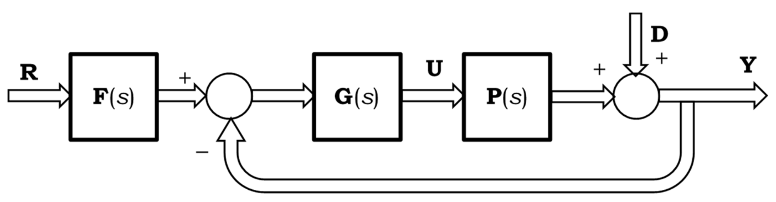
The main object of this paper is to compare feedback with and without the considerate pre-compensation above. The feedback controller matrix is assumed to be diagonal. The only cross-loop signal flow outside the given plant P is through the considerate pre-compensator matrix M, the design of which precedes the feedback loop design. A generic two-degree-of-freedom feedback control structure is given in Figure 1.
In Figure 1, the loop transfer matrix can be defined as . The system sensitivity matrix is accordingly . With this notation, the system output Y tracks the reference R and regulates the disturbance D as follows:
In much of the industrial application, scalar feedback loops are designed or tuned in some suitable sequence. That is equivalent to the feedback matrix in Figure 1 being diagonal:
With this diagonal controller, the loop transfer matrix L is non-diagonal. Nevertheless, with sufficiently high gain in all feedback loops, and Equation (22) simplifies to
With a diagonal F, this system tracks reference signals considerately (within the loop bandwidths). Some measure of robustness against plant uncertainty is automatically built-in, due to high gain feedback. There is no need for a (complex) pre-compensator design and tuning. Of course, there is no decoupling at frequencies near loop gain crossover and higher frequencies.
With the considerate pre-compensator, however, the controller is generally not diagonal:
With this considerate pre-compensation, the loop transfer matrix L is diagonal. To prove this, let us introduce the diagonal matrix
Now, Equation (25) can be written as
Hence, the loop transfer matrix becomes diagonal:
It follows that the sensitivity matrix S is diagonal and the entire control system in Equation (22) decomposes into n SISO systems when the reference filter F is diagonal. In other words, both reference tracking and disturbance regulation happen in a “considerate” manner without any crossfeed between the loops. This total decoupling is independent of the loop bandwidths or other aspects of the loop design. One of the problems is that this theoretical result is not necessarily achievable with fixed controllers because there is often some uncertainty in the interaction properties of P. However, a rigorous consideration of uncertainty is outside the scope of this paper.
Even though it may seem easier to design and tune non-interacting SISO loops, it is not clear that the regulating or tracking performance of these loops is necessarily superior to the performance of the simple feedback system with the diagonal controller in Equation (23). In order to get a feeling of what issues may be relevant, a few examples are analyzed below.
5. Examples
Example 1 (by Hovd and Skogestad [4]):
The plant is given as
The Bristol gains array is independent of frequency:
Feedback control of this system has been analysed by Hovd and Skogestad [4], who used it as a counterexample to the conventional pairing rule. It was further used by me in Ref. [3] to demonstrate the importance of sub-plant Bristol gains in the feedback loop design and tuning. If we pair the inputs and outputs according to i = j, then considerate control does not restrict the on-channel input or output scope, because all Bii are equal to 1. However, the off-channel interaction increases the required input scope by a factor of 5 and some input signs will be reversed too.
To summarize the design of three single loop Proportional plus Integral (PI) controllers by Hovd and Skogestad [4] and by me in Ref. [3], the following seems pertinent. Straightforward pairing on Bii = 1 yielded counter-intuitively poor regulating performance in all three loops. The achieved gain crossover frequency was . The non-minimum phase-lag zero in Equation (29) suggests (misleadingly perhaps) an order of magnitude of higher achievable gain crossover at . Input-output pairing on Bij = 5 yielded improved performance. Hovd and Skogestad [4] achieved between 0.1 and 0.3 in two of the loops while the third remained practically open with . I have designed three identical loops with in Ref. [3].
Common to all above design attempts was the appearance of large phase-angle deviations from the usual loop frequency response. Hence the low-frequency loop gain always remained counter-intuitively low. For example, the three identical loops, designed by me in Ref. [3], had a gain of merely 12 dB at . With a normally encountered slope of between −20 and −30 dB/decade near the gain crossover, this gain should have been somewhere in the range of 30 to 50 dB [5].
Now, let us first establish a considerate feedforward control structure and then design the three decoupled PI control loops. For this demonstration, we shall pair inputs and outputs on Bii = 5 (as recommended by Hovd and Skogestad [4] in a slightly different context). This is equivalent to reordering the plant outputs so that the last becomes the first:
The Bristol gains array is independent of frequency:
We use Equation (21) with . Hence, and the pre-compensator matrix is
There is no theoretical problem with implementing this compensator; hence, the compensated (considerate) plant transfer matrix is now
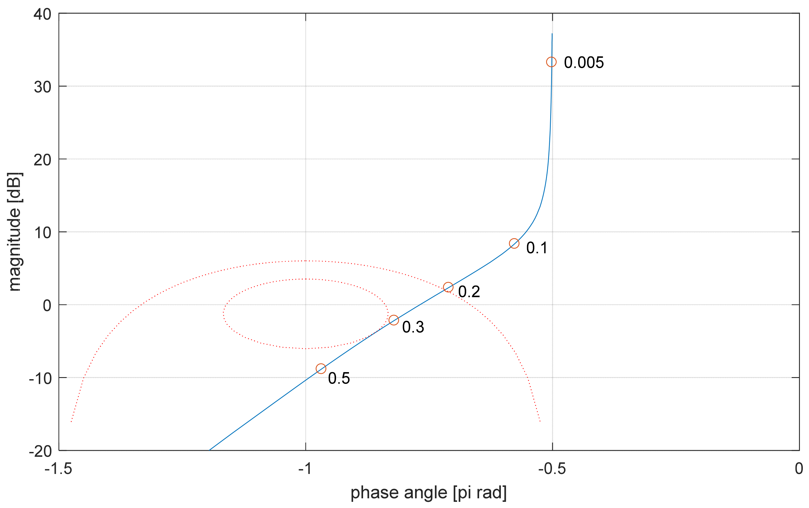
The following three PI controllers yielded identical loop transfer functions, as is shown in Figure 2:
Using some lead-lag compensation (such as is available in some commercial proportional plus integral plus so-called derivative controllers) would improve somewhat the gain cross-over frequency, but not by much.
Next, the achieved time-domain performance of the closed loop system is compared to that without the pre–compensator. The following PI controllers, for B11 = B22 = B33 = 5, are copied from Equation (5.21) of Ref. [3].
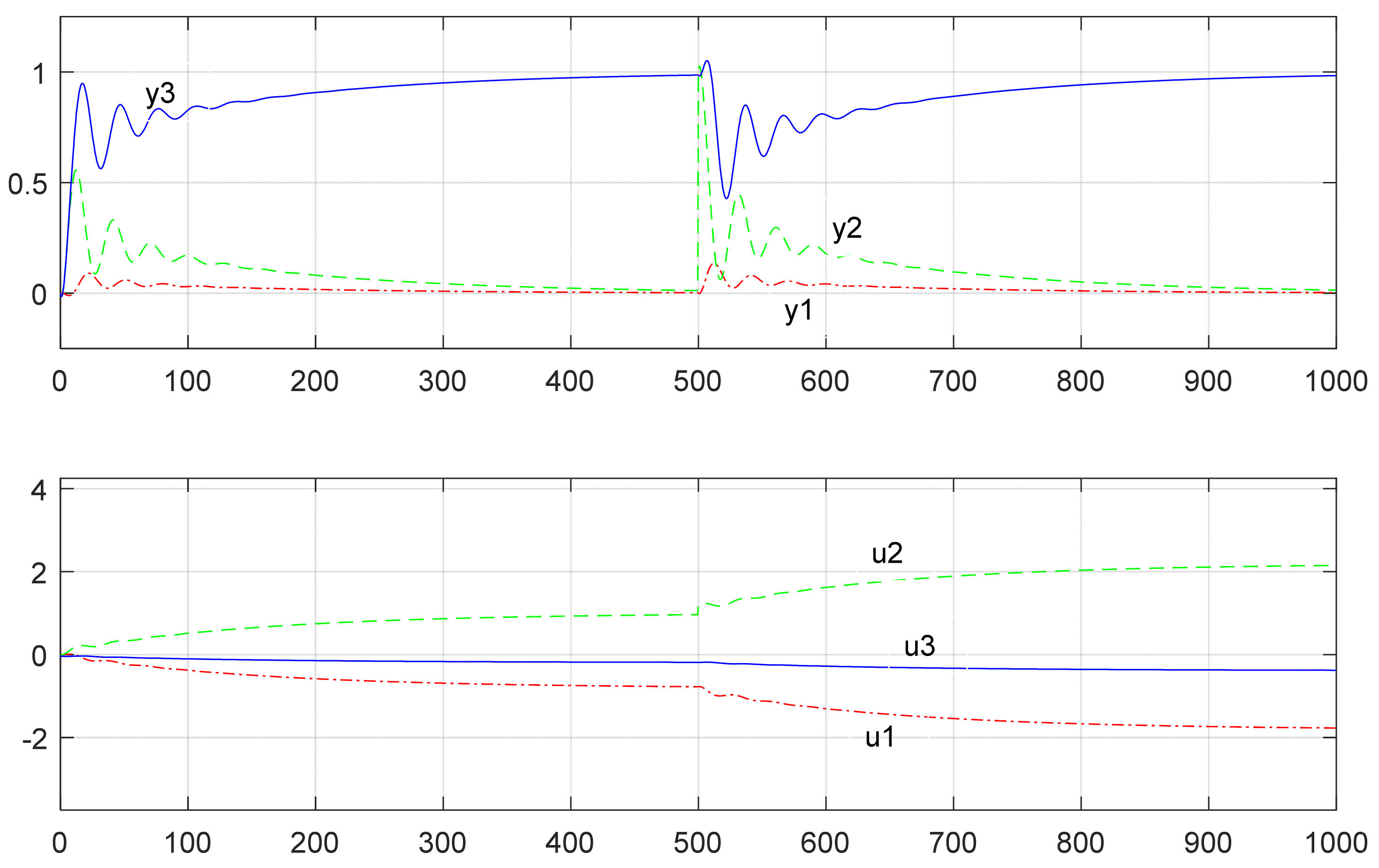
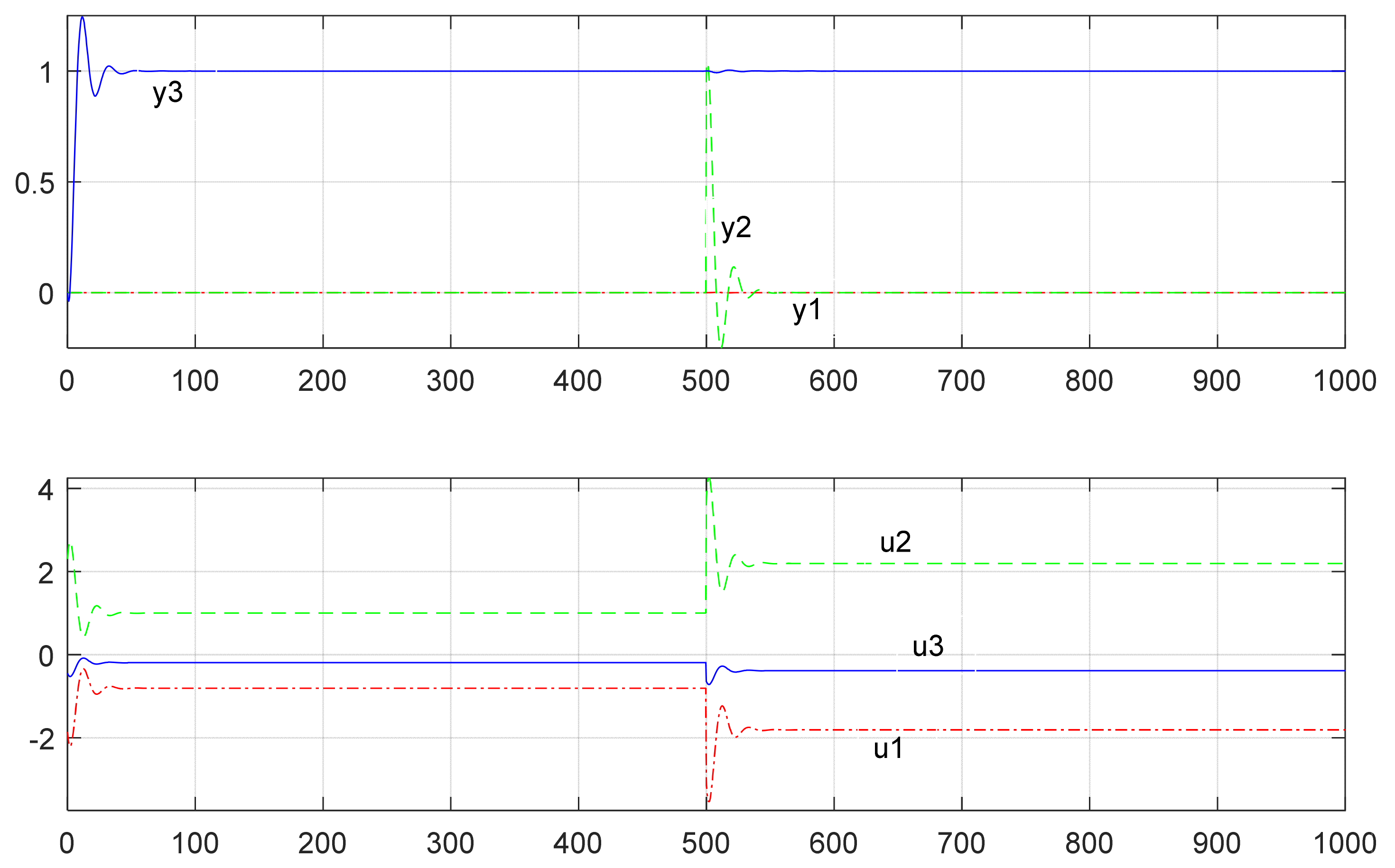
Figure 3 shows the corresponding reference and disturbance step responses. Figure 4 shows the reference and disturbance step responses with the considerate pre-compensation according to Equation (33). The PI controllers are given in Equation (35). Both control schemes result in considerate control eventually. The pre–compensator yields decoupled loops and; hence, it is easier to achieve better results, at least in this example.
Example 2: Considerate control with no “Bristol interaction”.
The plant is given as
The Bristol gains array is independent of frequency and indicates no interaction in the context of feedback loop design:
In this case, it was justified to follow the practitioner’s rule of pairing inputs and output on unit Bristol gains. Considerate control did not restrict the on-channel input or output scope. However, a fully considerate control would have required modification of the first input as follows.
From Equation (21), after a little calculation,
However, is non-causal and not implementable. To implement this de-coupler, it would need to be post-multiplied with something like
Thus, an implementable considerate pre-compensator would be given as
The compensated (considerate) plant transfer matrix would now be
In the original plant, the first loop gain cross-over frequency was limited to about 1, but the second loop had no theoretical bandwidth limitation. The following PI controllers were selected for comparison purposes:
In the considerately compensated plant as defined by Equation (42), however, both loops had the same gain crossover frequency limitation. A quick tuning yielded the two controllers as
Figure 5 and Figure 6 show various reference and disturbance step responses in the inconsiderate and considerate configurations, respectively.
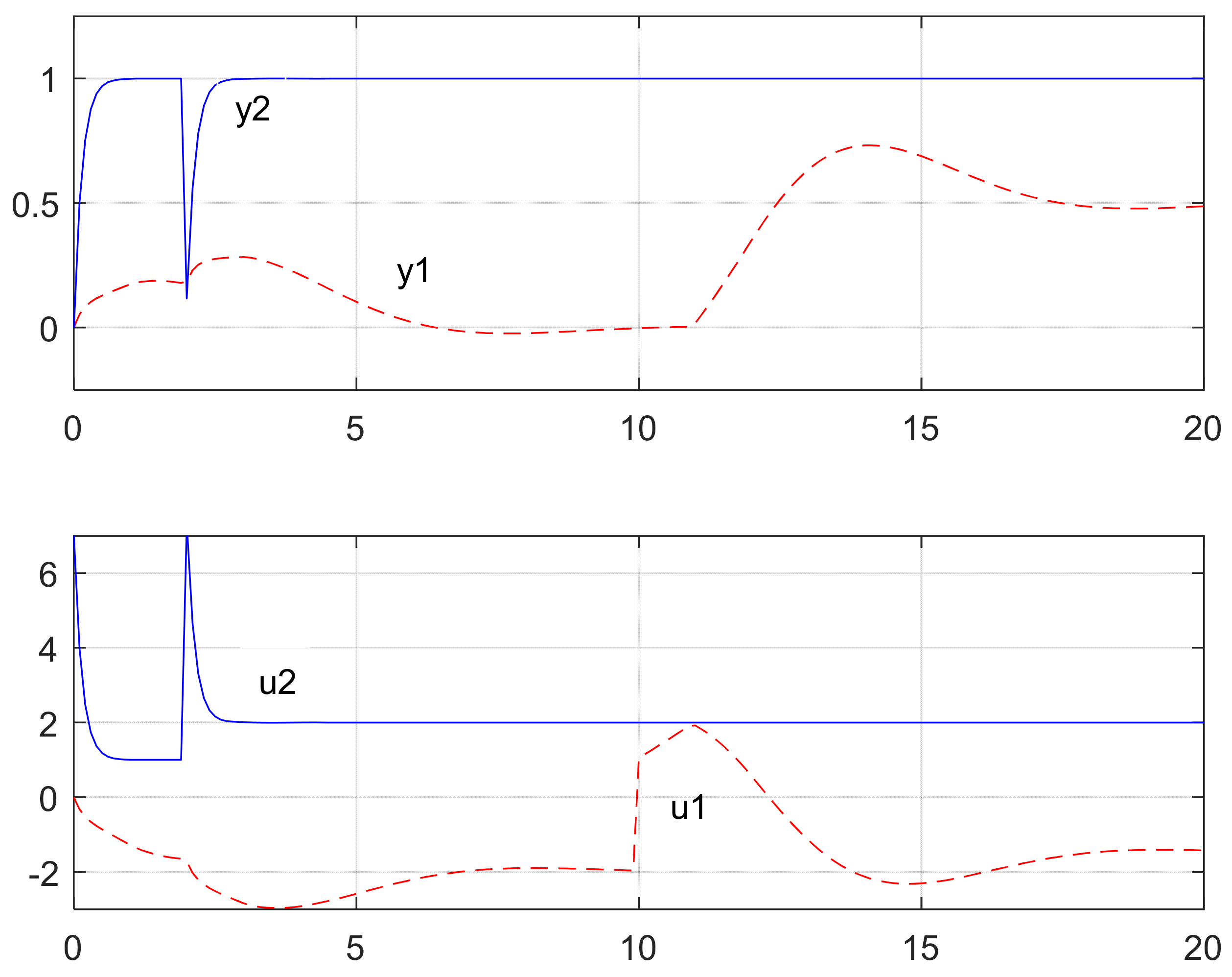
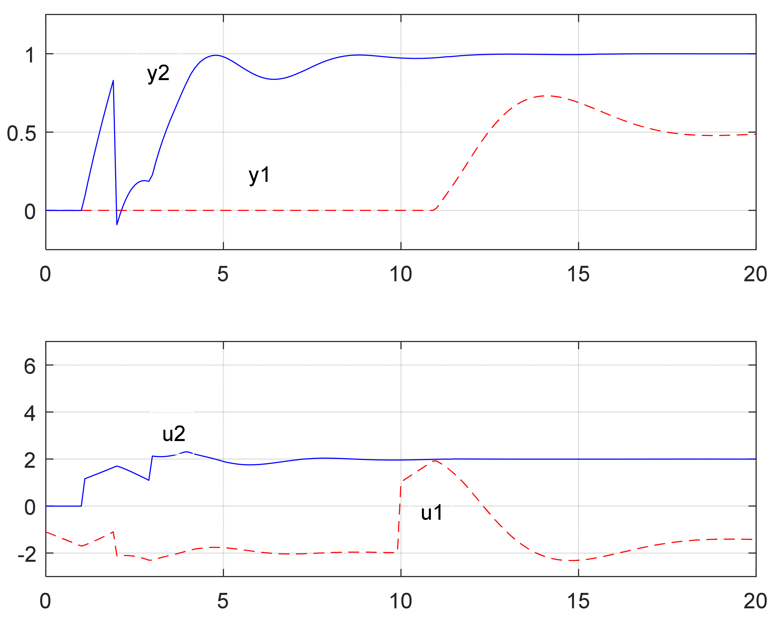
The inconsiderate regulation of y2 was significantly better than the considerate version. However, this performance came at the cost of disturbing y1. In this example, having consideration in the first loop, reduced performance of this loop.
Example 3 (by Yaniv and Gutman [6]):
The plant is given as
Note that element (3, 2) of this plant was reported with an error in Equation (5.5) of Ref. [3]. However, the Bristol gains array was reported correctly:
In Ref. [3] I have analyzed pure diagonal feedback. Using 2 × 2 sub-plant Bristol numbers in addition those in Equation (46) led to the recommendation of closing the second loop first, then the third loop. The first loop was to be tuned or designed last. This way, arbitrary bandwidth was achievable in the second and third loops. The first loop suffered the consequence of this plant’s right half–plane transmission zeros.
The following diagonal controller was recommended as one of the many arbitrary possibilities:
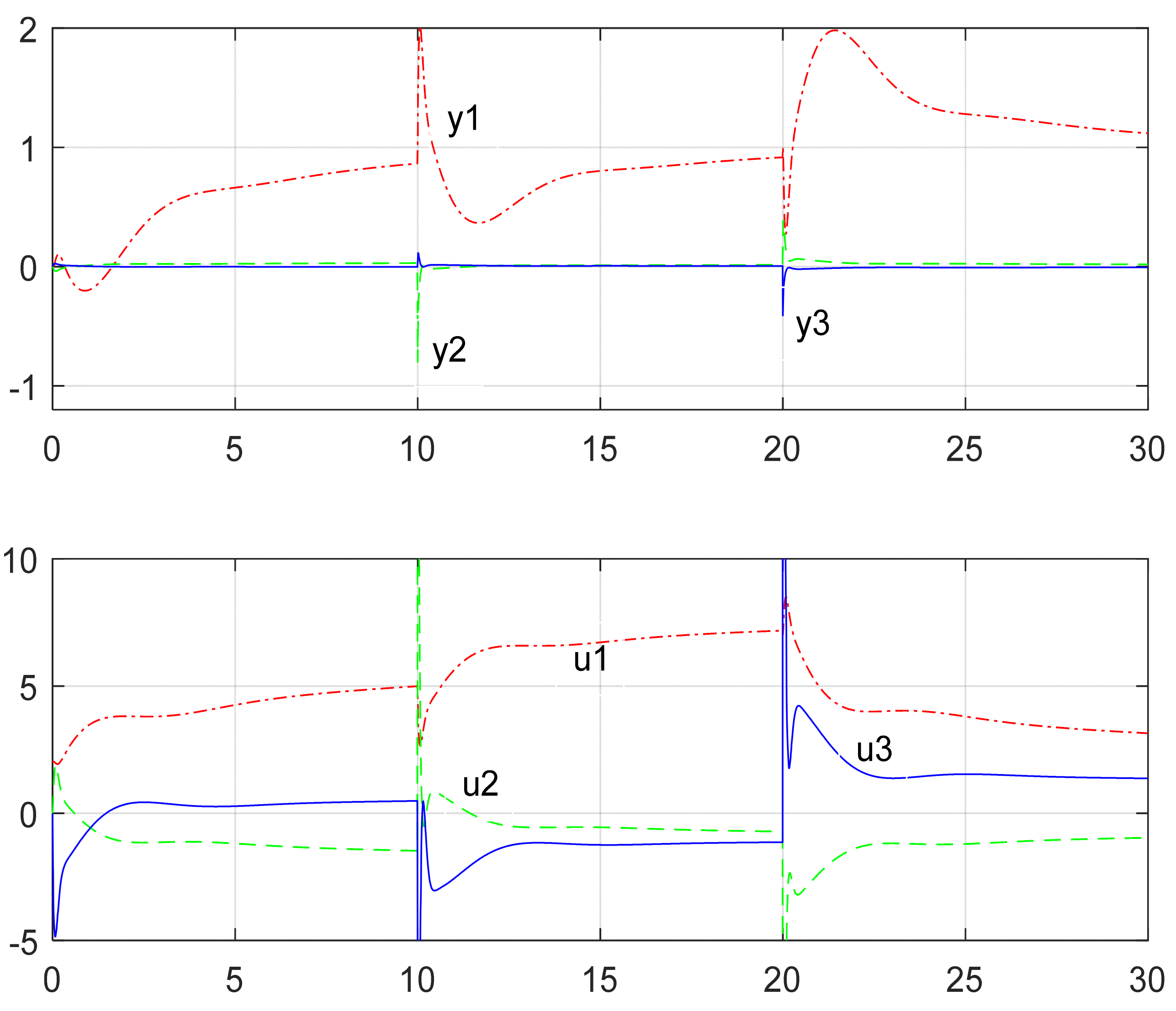
Of course, integral action could have been added to channels 2 and 3, but it was not necessary because of the arbitrarily high gain. Figure 7 shows various reference and disturbance step responses in this inconsiderate configuration.
We used Equation (21) with . Hence, and
There was no theoretical problem with implementing this compensator, so the compensated (considerate) plant transfer matrix became
The following three PI controllers maximized each of the three loop bandwidths with some reasonable gain and phase margins:
Figure 8 shows the step responses in this considerate configuration.
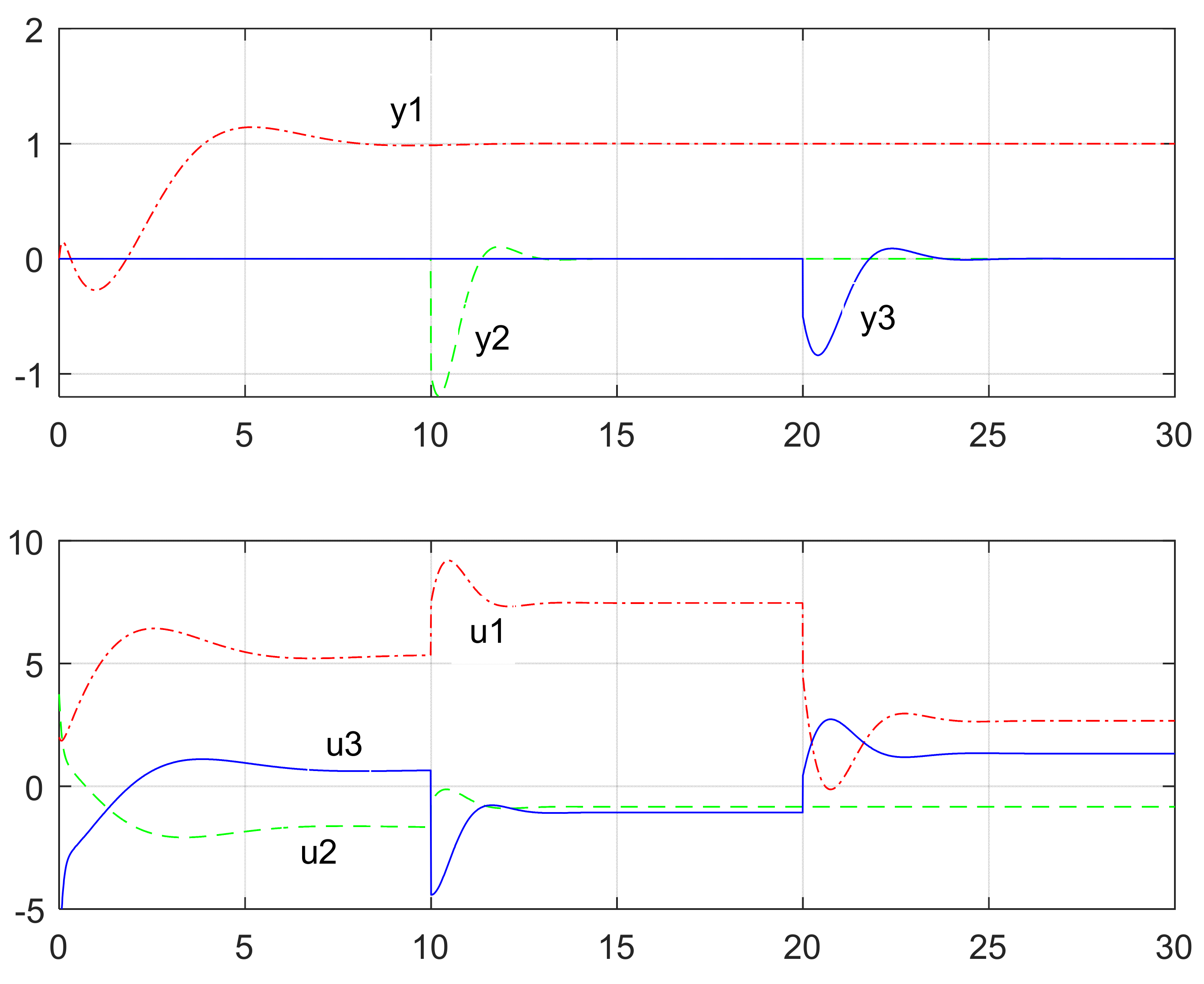
The inconsiderate regulation of y2 and y3 was significantly better than the considerate version. However, this performance was obtained at the cost of significant cross-channel disturbances in y1. This disturbance was not well regulated because the system interaction and high-gain in the second and third loops caused rather severe bandwidth limitation in the first loop.
In this example, having consideration eliminated the very large cross-channel disturbances. The price was the appearance of the right half-plane transmission zeros also in the second and third loops with the associated reduction of the second and third loop bandwidths and their regulating performance.
6. Discussion
Considerate control in interacting plants requires coordination of inputs in such a way that outputs of the plant are changed independently without consequential disturbance of other outputs. Considerate control can be achieved by fixed feedforward if plant uncertainty is negligible. It may be achieved by feedback alone, but not necessarily always and never over all frequencies.
Considerate control in interacting plants changes the achievable output or the required input ranges. This change is fully characterized by Bristol gains and it does not matter if the channel crossfeed is eliminated by feedforward pre-compensation or by sufficiently high-gain feedback within the loop bandwidths.
As the examples in Section 5 illustrated, considerate pre-compensation improves some aspects of MIMO tracking and regulating performance. However, degradation of other aspects–such as the appearance of additional non-minimum phase-lag—cannot necessarily be excluded.
Funding
This research did not receive any funding.
Data Availability Statement
Not applicable.
Conflicts of Interest
The author declares no conflict of interest.
References
- Eitelberg, E. Considerate control and Bristol gains. In Proceedings of the 2018 IEEE International Conference on the Science of Electrical Engineering (ICSEE), Eilat, Israel, 12–14 December 2018; pp. 1–5. [Google Scholar] [CrossRef]
- Bristol, E.H. On a new measure of interaction for multivariable process control. IEEE Trans. Autom. Control 1966, 11, 133–134. [Google Scholar] [CrossRef]
- Eitelberg, E. On multi-loop interaction and relative and Bristol gains. ASME J. Dyn. Syst. Meas. Control 2006, 128, 929–937. [Google Scholar] [CrossRef]
- Hovd, M.; Skogestad, S. Simple frequency-dependent tools for control system analysis, structure selection and design. Automatica 1992, 28, 989–996. [Google Scholar] [CrossRef]
- Eitelberg, E. The slope of a transfer function. Int. J. Control 2010, 73, 1249–1254. [Google Scholar] [CrossRef]
- Yaniv, O.; Gutman, P.-O. Crossover frequency limitations in MIMO nonminimum phase feedback systems. IEEE Trans. Autom. Control 2002, 47, 1560–1564. [Google Scholar] [CrossRef]
Figure 1.
A two-degree-of-freedom MIMO feedback control system block diagram. R, U, D, and Y are the system reference, plant input, plant disturbance, and system output vectors respectively. Signal flow direction is shown with the arrows on double lines and the circles indicate summation of entering signals. P is the given system transfer matrix. G is the to be designed feedback controller matrix. F is the feed forward reference filter matrix – it may be used for some engineering purposes, but is assumed to be a unit matrix in the following examples.

Figure 2.
Identical loop frequency responses on the logarithmic complex plane with considerate input–output pairing on B11 = B22 = B33 = 5. The vertical axis shows the dB magnitude of the loop transfer function and horizontal axis shows the loop transfer function phase angle in terms of π radians. Five frequency values (in rad/s) are indicated on the blue frequency response. The closed-loop sensitivity magnitudes of 0 dB and 6 dB are indicated with the dotted red lines. The red 6 dB sensitivity oval was used as the stability margin for the shown design.

Figure 3.
Inconsiderate reference tracking and disturbance regulation. Upper plot shows the system outputs y1, y2, and y3, as functions of time. Lower plot shows the system inputs u1, u2, and u3, as functions of time. All references and output disturbances in Figure 1 are zero, except and , where is the unit step function (or rather distribution) at time t = 0.

Figure 4.
Reference tracking and disturbance regulation with considerate pre-compensation. Upper plot shows the system outputs y1, y2, and y3, as functions of time. Lower plot shows the system inputs u1, u2, and u3, as functions of time. All references and output disturbances in Figure 1 are zero, except and , where is the unit step function (or rather distribution) at time t = 0.

Figure 5.
Reference tracking and disturbance regulation without de-coupling. Upper plot shows the system outputs y1 and y2 as functions of time. Lower plot shows the system inputs u1 and u2 as functions of time. The references in Figure 1 are and . The output disturbances in Figure 1 are and , where is the unit step function (or rather distribution) at time t = 0.

Figure 6.
Reference tracking and disturbance regulation with considerate pre–compensation. Upper plot shows the system outputs y1 and y2 as functions of time. Lower plot shows the system inputs u1 and u2 as functions of time. The references in Figure 1 are and . The output disturbances in Figure 1 are and , where is the unit step function (or rather distribution) at time t = 0.

Figure 7.
Inconsiderate reference tracking and disturbance regulation. Upper plot shows the system outputs y1, y2 and y3 as functions of time. Lower plot shows the system inputs u1, u2 and u3 as functions of time. The references in Figure 1 are and . The output disturbances in Figure 1 are are , and , where is the unit step function (rather distribution) at time t = 0.

Figure 8.
Reference tracking and disturbance regulation with considerate de-coupling. Upper plot shows the system outputs y1, y2 and y3 as functions of time. Lower plot shows the system inputs u1, u2 and u3 as functions of time. The references are in Figure 1 are and . The output disturbances in Figure 1 are , and , where is the unit step function (rather distribution) at time t = 0.

Publisher’s Note: MDPI stays neutral with regard to jurisdictional claims in published maps and institutional affiliations. |
© 2021 by the author. Licensee MDPI, Basel, Switzerland. This article is an open access article distributed under the terms and conditions of the Creative Commons Attribution (CC BY) license (https://creativecommons.org/licenses/by/4.0/).
Share and Cite
MDPI and ACS Style
Eitelberg, E. Considerate Regulation of Output Disturbances. Physics 2021, 3, 173-186. https://0-doi-org.brum.beds.ac.uk/10.3390/physics3020014
AMA Style
Eitelberg E. Considerate Regulation of Output Disturbances. Physics. 2021; 3(2):173-186. https://0-doi-org.brum.beds.ac.uk/10.3390/physics3020014
Chicago/Turabian StyleEitelberg, Eduard. 2021. "Considerate Regulation of Output Disturbances" Physics 3, no. 2: 173-186. https://0-doi-org.brum.beds.ac.uk/10.3390/physics3020014