Fluctuating Number of Energy Levels in Mixed-Type Lemon Billiards


1
Faculty of Mathematics and Physics, University of Ljubljana, Jadranska 19, SI-1000 Ljubljana, Slovenia
2
CAMTP—Center for Applied Mathematics and Theoretical Physics, University of Maribor, Mladinska 3, SI-2000 Maribor, Slovenia
*
Author to whom correspondence should be addressed.
†
Deceased.
Physics 2021, 3(4), 888-902; https://0-doi-org.brum.beds.ac.uk/10.3390/physics3040055
Submission received: 15 July 2021
/
Revised: 10 August 2021
/
Accepted: 16 August 2021
/
Published: 2 October 2021
(This article belongs to the Special Issue Dedication to Professor Michael Tribelsky: 50 Years in Physics)
Abstract
:In this paper, the fluctuation properties of the number of energy levels (mode fluctuation) are studied in the mixed-type lemon billiards at high lying energies. The boundary of the lemon billiards is defined by the intersection of two circles of equal unit radius with the distance between the centers, as introduced by Heller and Tomsovic. In this paper, the case of two billiards, defined by , is studied. It is shown that the fluctuation of the number of energy levels follows the Gaussian distribution quite accurately, even though the relative fraction of the chaotic part of the phase space is only 0.28 and 0.16, respectively. The theoretical description of spectral fluctuations in the Berry–Robnik picture is discussed. Also, the (golden mean) integrable rectangular billiard is studied and an almost Gaussian distribution is obtained, in contrast to theory expectations. However, the variance as a function of energy, E, behaves as , in agreement with the theoretical prediction by Steiner.
1. Introduction
The purpose of this paper is to analyze the energy spectra of two characteristic complex mixed-type lemon billiards within the scope of quantum chaos. The boundary of the lemon billiards is defined by the intersection of two circles of equal unit radius with the distance between the centers, as introduced by Heller and Tomsovic in 1993 [1,2]. The present study represents a continuation of our recent paper [3] on the classical and quantum ergodic billiard () with strong stickiness effects, from the family of lemon billiards, as well as on three simple mixed-type lemon billiards with only one regular region, surrounded by a uniform chaotic sea without stickiness regions, namely, with the shape parameters [4].
In the present paper, two lemon billiards with the shape parameters are studied. These lemon billiards are mixed-type billiards with several independent regular regions embedded in a chaotic sea with no significant stickiness regions, which serve as examples of systems with a complex divided phase space. These lemon billiards were selected by the criterion of the maximally complex chaotic component generated by a single chaotic orbit. The discovery of the present and past physically and dynamically different and interesting lemon billiards has only been made possible thanks to the recent extensive analysis of Lozej [2]. The entire family of classical lemon billiards for a dense set of about 4000 values of (in steps of ) was systematically analyzed as for the corresponding phase space structure and stickiness effects. It must be emphasized that although all the lemon billiards belong to the same family of billiards as for the mathematical definition, individually, the lemon billiards have quite different, in fact, very rich, dynamical properties, important in the classical and quantum context.
A general introduction to the subjects in quantum chaos, related to this study, can be found in [3]. Let us also mention the books by Stöckmann [5] and Haake [6] on general quantum chaos and the recent reviews [7,8] on stationary quantum chaos in generic (mixed-type) systems.
The main purpose of the present paper is to analyze the two selected quantum lemon billiards of and , with the goal to study the energy spectra, while the structure of the Poincaré–Husimi functions in the phase space, the separation of the regular eigenstates and chaotic eigenstates, as well as the localization properties of the chaotic eigenstates and their statistics will be treated separately [9].
The main results are as follows. The energy spectra are calculated by the scaling method of Vergini–Saraceno [10] in two versions, one based on the plane waves and the other one based on the circular waves (Bessel functions for the radial part and trigonometric functions for the angular part). This is done for high-lying eigenstates with the wavenumber k (in the specific units) for up to 300,000 consecutive levels for each of the four symmetry classes (odd-odd, odd-even, even-odd, and even-even). The energy of the level at k is . It turns out that about 0.1% of the levels are lost for technical reasons, which is a known and experienced fact in numerically calculating billiard spectra with the scaling method, while the accuracy of individual levels is better than 1% of the mean energy level spacing. The spectral statistics are found to be stable with respect to these losses. The cumulative (integrated) energy level density (spectral staircase function) is well described by the Weyl formula (with the leading area term and the perimeter term) if there are no missing levels. Then the fluctuations of the actual staircase function around the Weyl function, the difference , and the distribution are studied. In the literature, is called mode fluctuation [11,12,13,14]. Due to the lost levels, this difference has a drift to negative values and fluctuates around the mean value. In order to separate the drift and the fluctuations, the quantity , where is the local average of over 100 consecutive levels, is investigated. Then, the distribution of for about 300,000 levels of each symmetry class separately, starting at , within the interval approximately is studied. One finds that the distribution of w follows a Gaussian distribution fairly well, which is a surprising result as the two billiards have the relative fraction of the chaotic phase space of only 0.28 and 0.16, respectively. For comparison, also the entirely regular, integrable, case of the maximally irrational rectangular billiard is investigated and it is surprisingly found an almost Gaussian distribution for w, but with the variance rising linearly with k, as generally predicted by the theory of Steiner [11,12,13,14], while the distribution itself in integrable systems is predicted to be nonuniversal, varying from case to case, which here is not confirmed. The validity of the theoretical predictions has also been checked in experiments with superconducting microwave billiards [15]. Finally, the level spacing distribution for the two lemon billiards is presented which provides good agreement with the Berry–Robnik–Brody distribution.
The paper is organized as follows. In Section 2, the definition are given and classical dynamical properties of the lemon billiards are examined. In Section 3, the analysis of the fluctuation quantity is performed. In Section 4, the statistical analysis of the entire energy spectra is made by calculating the level spacing distribution, . In Section 5, the results are discussed and conclusions are presented.
2. The Lemon Billiards and Their Phase Portraits
The family of lemon billiards was introduced by Heller and Tomsovic in 1993 [1] and has been studied in a number of papers [16,17,18,19,20], most recently, in [2,3,4,21]. and in the recent studies [3,4] by us. The lemon billiard boundary is defined by the intersection of two circles of equal unit radius with the distance between the centers, , being less than the diameters and , and is given by the following implicit equations in Cartesian coordinates:
As usual, the canonical variables are used to specify the location, s, and the momentum component, p, on the boundary at the collision point. Namely, the arc length, s, is counted in the mathematical positive sense (counterclockwise) from the point as the origin, while p is equal to the sine of the reflection angle ; thus , as . The bounce map is area preserving as in all billiard systems [22]. Due to the two kinks, the Lazutkin invariant tori (related to the boundary glancing orbits) do not exist. The period-2 orbit connecting the centers of the two circular arcs at the positions and is always stable (and therefore surrounded by a regular island) except for the case , where it is a marginally unstable periodic orbit, the case being ergodic and treated by us earlier [3].
The circumference of the entire billiard, , is given by:
The area of the billiard is:
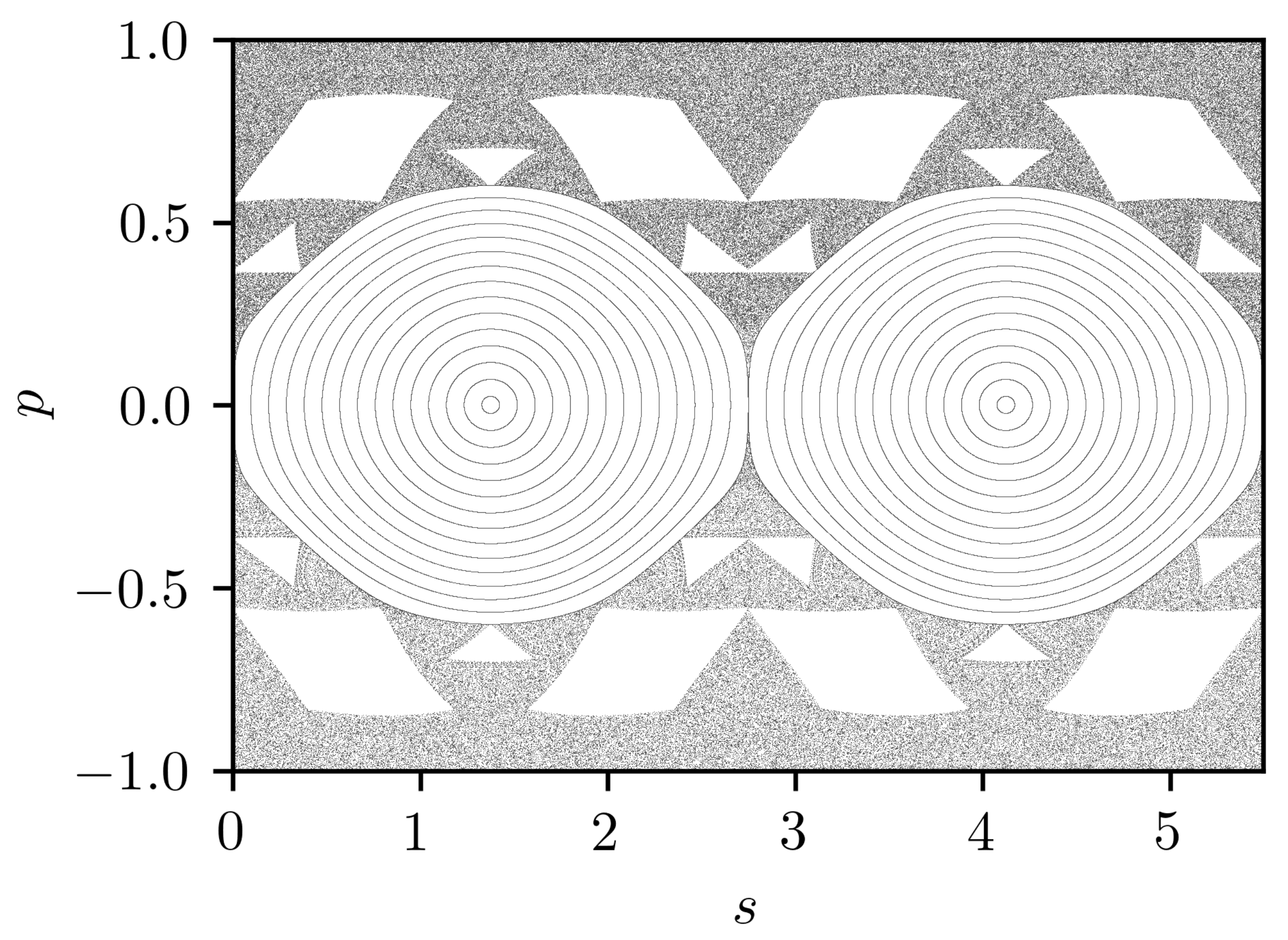
The structure of the phase space is shown in Figure 1 for the lemon billiard of , with . The relative fraction of the area of the chaotic component of the bounce map is , while the relative fraction of the phase space volume of the same chaotic component is , the Berry–Robnik parameter. Three independent regular island chains are clearly visible, the largest one around the period-2 orbit, which is densely covered by the invariant tori, with no visible thin chaotic layers inside. Let us denote the largest island chain by L, the second largest one by M, and the smallest one by S. The relative phase space volume of all three regular regions taken together is . The chaotic sea is quite uniform, with no significant stickiness regions, and is generated by a single chaotic orbit.
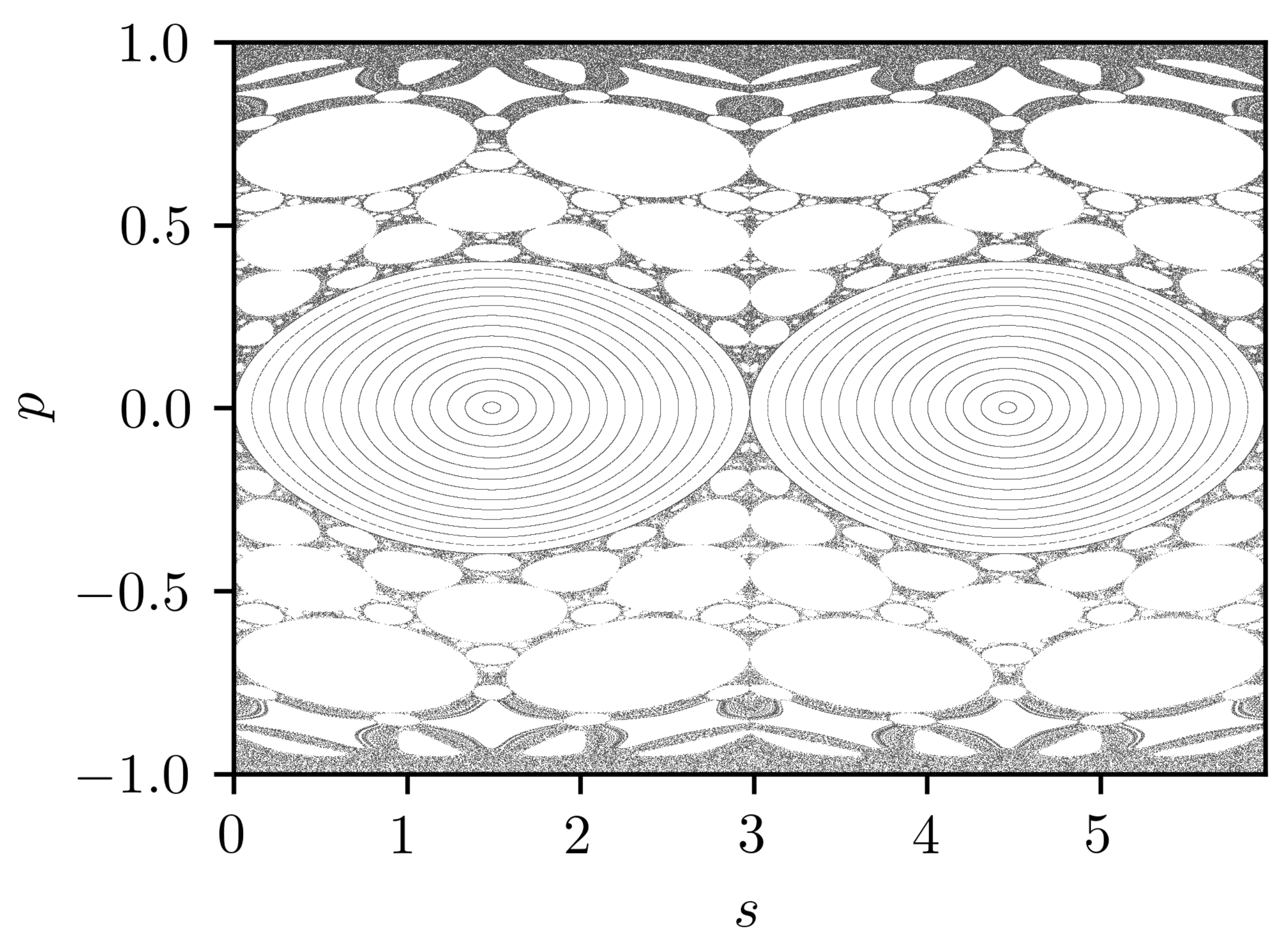
The structure of the phase space, as shown in Figure 2 for the lemon billiard of , is more complex. Here, . The relative fraction of the area of the chaotic component of the bounce map is , while the relative fraction of the phase space volume of the same chaotic component is . Thus, the relative phase space volume fraction of the complementary regular regions is . In this case also, the chaotic sea is rather uniform, with no significant stickiness regions, and is generated by a single chaotic orbit, creating a very complex structure, perhaps mimicking stickiness in some thin regions. Both billiards are clearly of the Kolmogorov-Arnold-Moser (KAM) type, generic systems; examples of stochastic transition were studied already in [23].
One can conclude that the two cases are interesting to verify the Berry–Robnik picture of quantum billiards [24], including the possible quantum localization of chaotic eigenstates, leading to the Berry–Robnik–Brody level spacing distribution and the universal statistical properties of the localization measures [4,9], as there are no significant stickiness effects, based on the results of the analysis of the recurrence time statistics in [2], unlike in the ergodic case, , studied in [3].
3. The Energy Spectra and the Fluctuation of the Number of Energy Levels
Let us now turn to the quantum billiard described by the stationary Schrödinger equation in the chosen units () given by the Helmholtz equation:
with the Dirichlet boundary conditions , and the energy is . Here ℏ is the reduced Planck constant and m is the mass of the particle.
The mean number of energy levels below is determined quite accurately, especially at large energies, asymptotically exact, by the celebrated Weyl formula (with perimeter corrections) using the Dirichlet boundary conditions, namely:
where “c.c.” stays for small constants, determined by the corners and the curvature of the billiard boundary, which differentially play no role. Thus, the mean density of levels is equal to:
The numerical method used here to solve the Helmholtz equation is based on the Heller’s plane wave decomposition method and the Vergini–Saraceno scaling method [10,25]. Both versions of the Vergini–Saraceno method are implemented, namely, the one, based on plane waves, and the other one, based on the circular waves, and the same results are obtained within an accuracy of 0.1% of the mean level spacing. As mentioned, typically at most about 0.1% of the levels are lost. The numerical accuracy was checked by the convergence test, by varying the method’s parameters (the number of basis waves and the number of nodes on the boundary).
The billiard considered has two reflection symmetries; thus, the eigenstates have four symmetry classes: odd-odd, odd-even, even-odd, and even-even. For the purpose of analyzing the spectral statistics and the wave functions, let us consider only the quarter billiard. In this case, the Weyl formula for the four symmetry classes reads:
where is defined for each of the above-defined symmetry classes as follows::
where and . Note that summing up the four contributions in Equation (7) with Equation (8), one obtains the Weyl formula for the entire spectrum Equation (5). For each symmetry class for each of the two billiards, about 300,000 levels were calculated and the difference, , was studied between the staircase function, , and the Weyl function, .
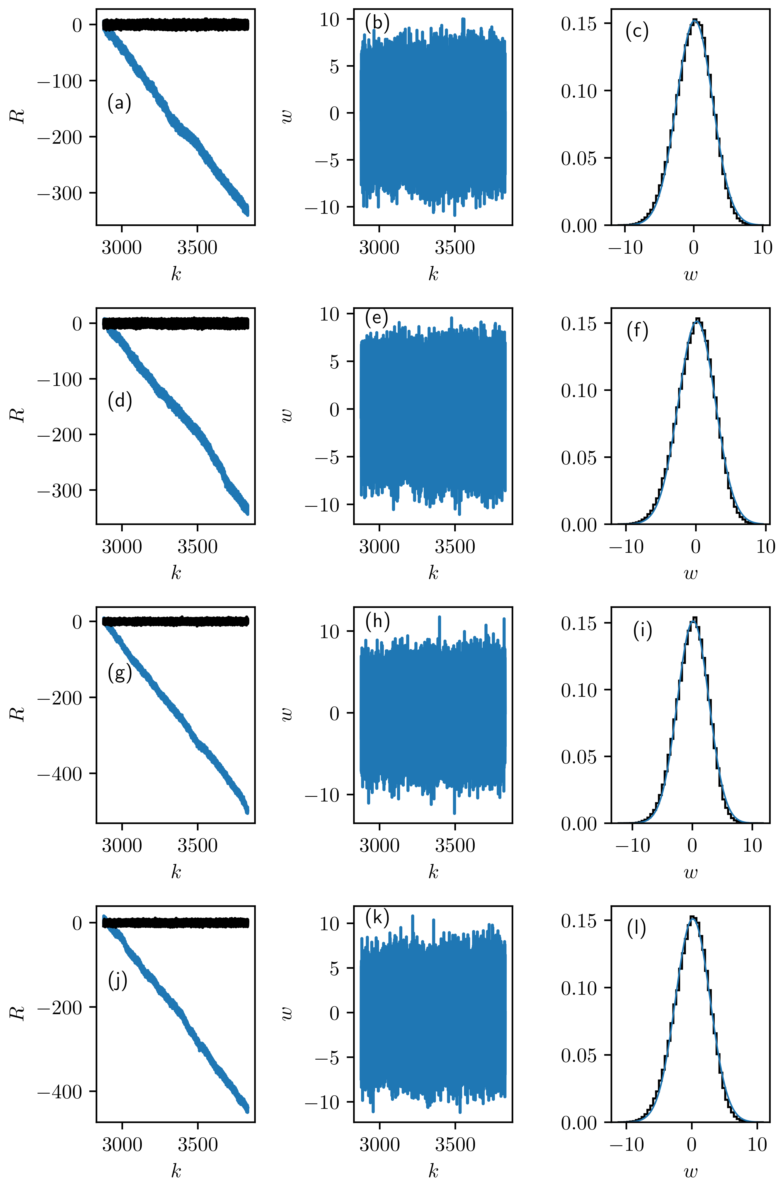
Figure 3 shows the results for the billiard. It is clear that decreases linearly with k due to the numerical loss of the levels. Typically, about 0.1% of the levels are missing. In order to study the fluctuation properties, one needs to subtract the local mean value, , obtained by averaging over 100 consecutive levels, and then analyze the resulting fluctuation quantity, . The agreement with the Gaussian distribution is extremely good which is surprising, as the billiard is predominantly regular, with only 28% of the chaotic component. Steiner’s theory [11,12,13,14] predicts a Gaussian distribution only for entirely chaotic (ergodic) systems, while the distribution of the fluctuation quantity, w, in integrable systems is expected to be nonuniversal. In the mixed-type case, the distribution of w should be in between, which here is not the case. Moreover, even for the rectangle as an example of the integrable systems, an (almost) Gaussian distribution is found (see below).
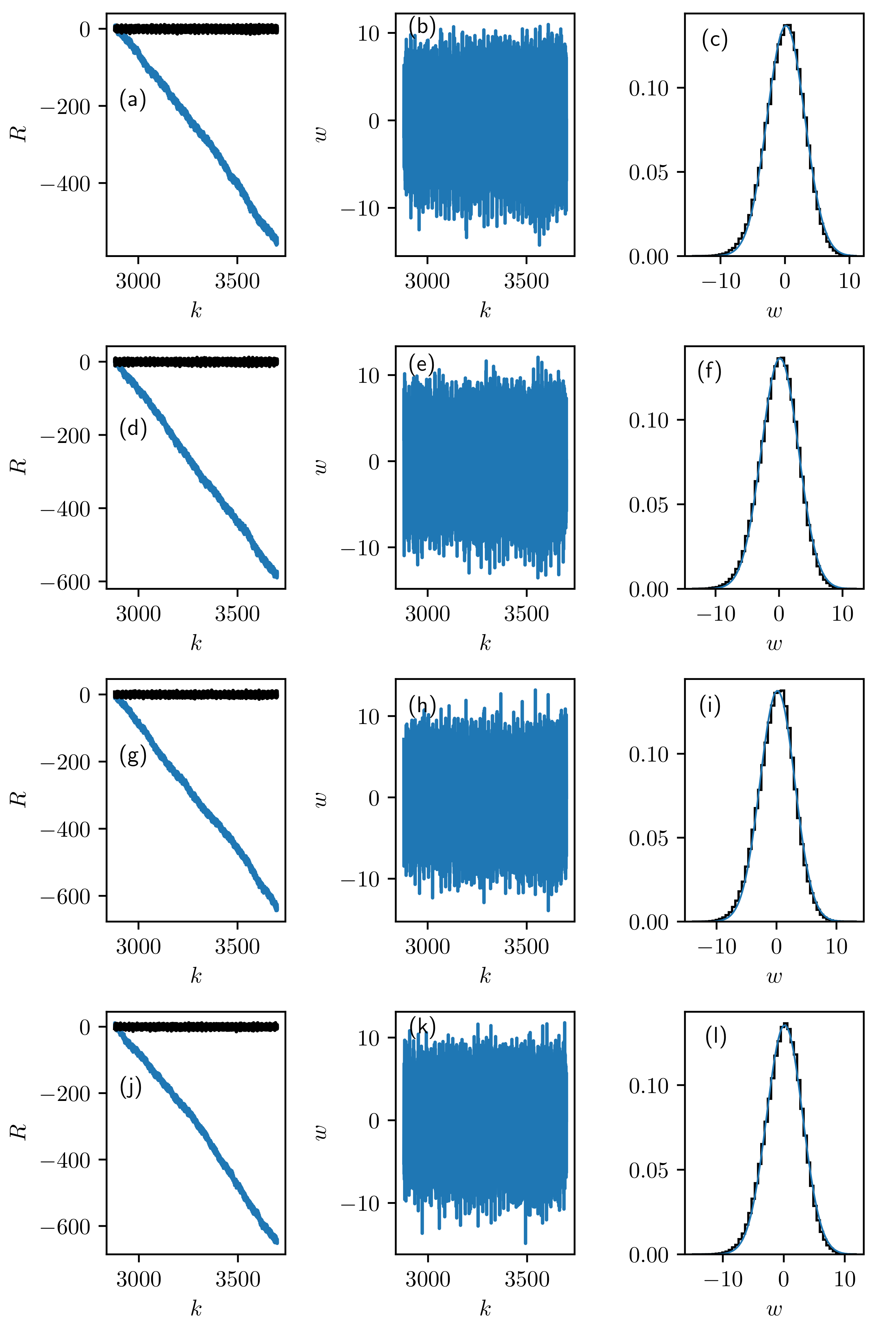
The same analysis was performed for the case of the B = 0.083 billiard, and the results are shown in Figure 4, and lead to the same conclusions.
The local averaging procedure over 100 consecutive levels is, of course, somewhat arbitrary. Therefore, the results were checked for levels. In all cases, the distribution was found to represent Gaussian extremely well. The standard deviation at each level number keeps the same value for all parities, but increases slowly with the number of levels such that for for , one gets , respectively. For the billiard, the corresponding values are: .
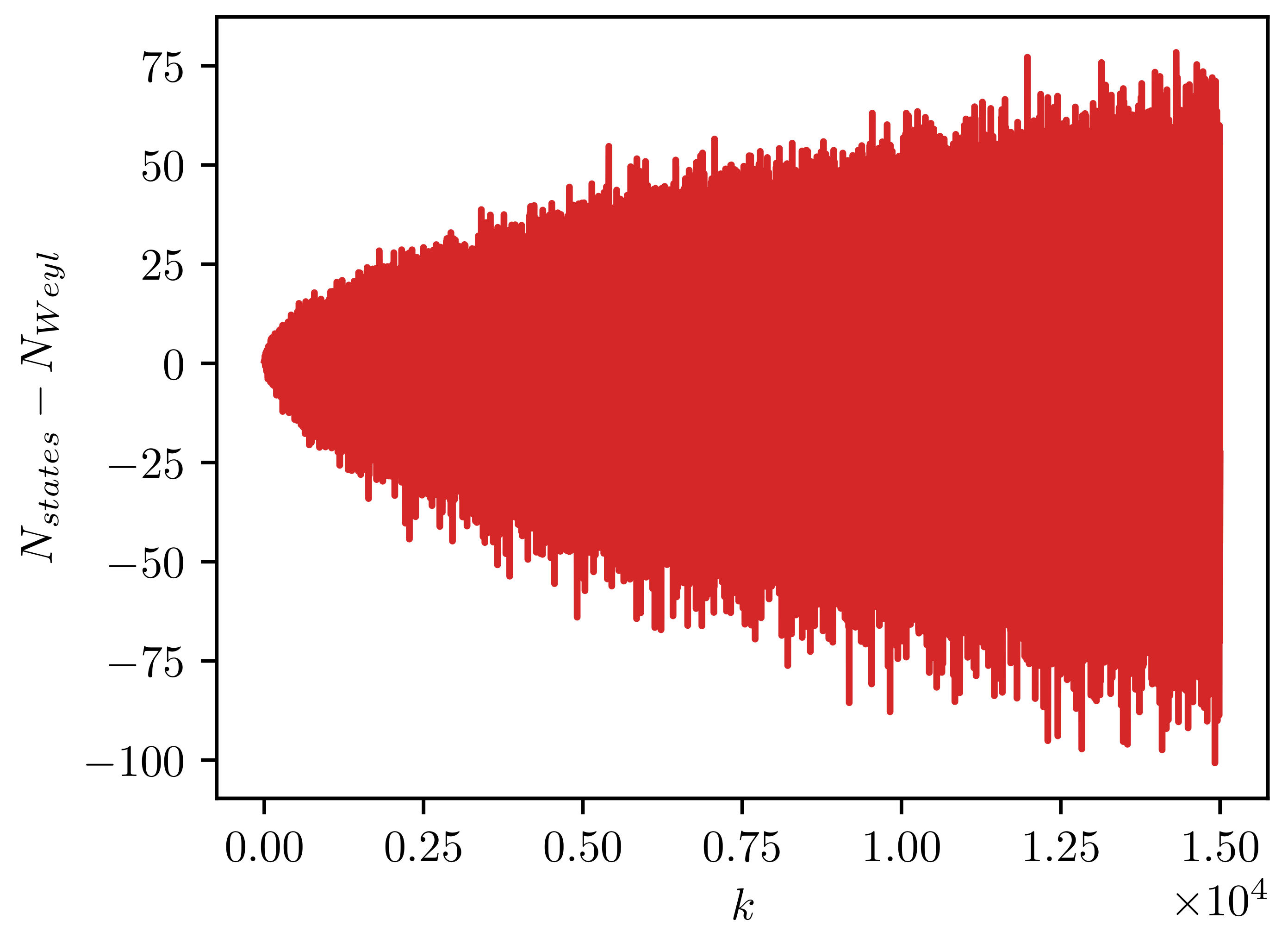
In order to explore an integrable, entirely regular system, an example of the maximally irrational rectangle billiard was studied whose aspect ratio was taken the golden mean . The spectrum in this case is known analytically, and is exact: , where l and n are two positive integers. Figure 5 shows the fluctuation quantity , which has no drift, because the spectrum is exact (no lost levels) over a wide range of k.
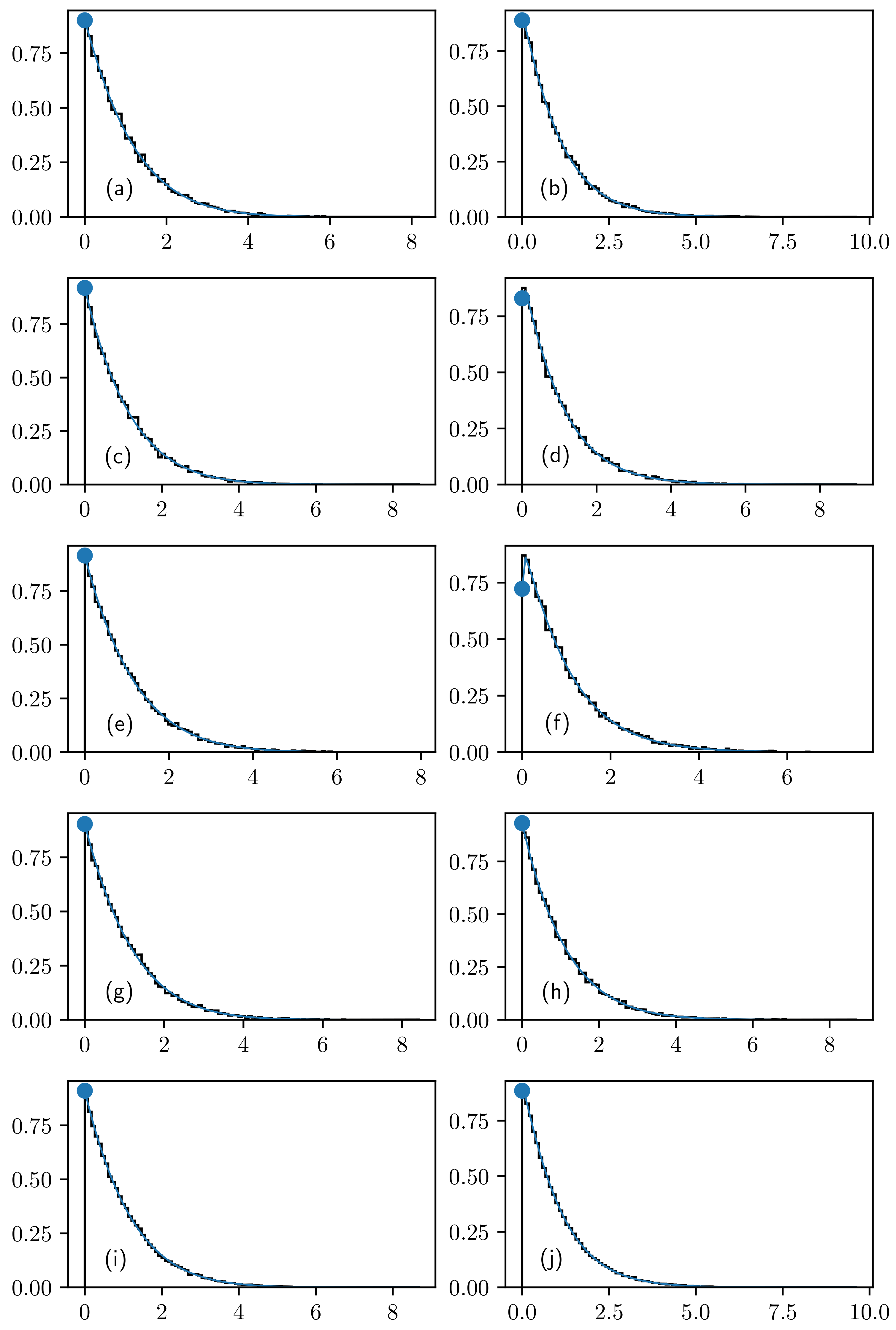
The corresponding distributions at various wavenumber k intervals starting at are shown in Figure 6. Each histogram comprises about 100,000 objects. They are surprisingly close to a Gaussian distribution, contrary to the theoretical expectation, and thus, the distribution is just close to the case of ergodic chaotic systems. Therefore, the distribution of the number of energy levels (distribution of mode fluctuations) is not a good criterion to distinguish ergodic chaotic systems from the regular integrable systems. In Table 1, the data for the mean, , standard deviation, , skewness, and kurtosis are given.
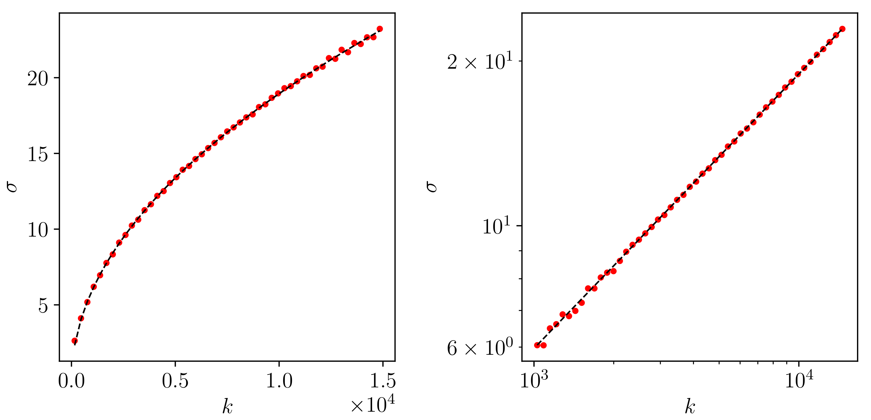
In Figure 7, the standard deviation of the distributions of w is plotted as a function of k, which clearly accurately follows the prediction by Steiner [11,12,13,14], namely the standard deviation rises as , shown also in the log-log plot, and the variance is a linear function of k. Therefore, the dependence of the variance on k is a good signature of chaos, unlike the distribution itself: in ergodic chaotic systems, the standard deviation behaves as .
4. Level Spacing Distribution for the Entire Spectrum
One of the most important statistical measures of the (unfolded) energy spectra is the level spacing distribution, . For integrable systems, one gets Poissonian statistics and , while for classically ergodic (fully chaotic) systems the Gaussian orthogonal ensemble (GOE) of random matrix theory applies. The Wigner distribution (Wigner surmise) is 2-dimensional GOE distribution and is a very good approximation for the GOE level spacing distribution (infinite-dimensional),
There is a general useful relationship, namely, one using the gap probability, , being the probability of having no level on an arbitrary interval of length S: the level spacing distribution is, in general, equal to the second derivative of the gap probability, .
For Poisson statistics: , while for the Wigner distribution, one finds:
For mixed-type systems, there is typically one dominant chaotic component with the relative density of levels (equal to the relative fraction of the chaotic phase space volume), while the complement is typically a regular component of relative density, . If the regular and chaotic levels superimpose statistically independent of each other, then obviously, the gap probability factorizes:
and therefore, in this case, the level spacing distribution is given by the Berry–Robnik (BR) formula [24]:
The above statements are true provided the Heisenberg time is larger than any classical transport time in the system [8]. (The Heisenberg time is defined as , where is the mean energy level density, also the reciprocal mean energy level spacing.) If this is not the case, the chaotic eigenstates can be quantum (or dynamically) localized, which implies localized chaotic Poincaré–Husimi functions in the phase space. The level spacing distribution for such localized chaotic eigenstates becomes (approximately) the known Brody distribution [26,27]:
where by the normalization of the total probability and the first moment, one gets:
where is the Gamma function. The Brody distribution interpolates the exponential and Wigner distribution as goes from zero to one. The important feature of the Brody distribution is the fractional level repulsion effect, meaning the power law at small S, . The corresponding gap probability is:
where , and is the incomplete Gamma function:
Here, the only parameter is , the level repulsion exponent in (13), which measures the degree of localization of the chaotic eigenstates: if the localization is maximally strong, the eigenstates practically do not overlap in the phase space (of the Wigner functions), and one finds and a Poissonian distribution, while in the case of maximal extendedness (no localization), one finds and the GOE statistics of levels applies. Thus, by replacing by , the Berry–Robnik–Brody (BRB) distribution is obtained which generalizes the BR distribution (12) such that the localization effects in chaotic eigenstates are included [28]. Note that in the semiclassical limit, or , the Heisenberg time becomes arbitrarily large (larger than any classical transport time), the localization effects of chaotic eigenstates disappear, and the BRB distribution becomes the BR distribution. However, the theoretical derivation of the Brody distribution for the localized chaotic states remains an important open problem. Furthermore, while the local behavior at small S, described by the power law , is certainly correct, the global feature of the Brody distribution is surely approximate, although empirically is well founded.
In Figure 8, the present study, the classical transport time of the billiards is very short; therefore, one expects , and the level spacing distribution is almost BR one (12). Thus, in the level statistics, one does not detect large localization effects. For the spectral unfolding procedure, the Weyl formula, Equation (5), is used, which at high energies is quite accurate.
Figure 8, shows the level spacing distributions for the two billiards—one of (left column), and another one of (right column)—for the spectral stretches each about 20,000 levels long, starting at , for each parity: even-even even-odd, odd-even and odd-odd and for all four parities together (about 80,000 levels), each of them along with the best fitting BRB distribution.
As one can see, in the case of , Figure 8a,c,e,g,i, the parameter is very close to one, while the parameter is close to the classical value, , being the relative fraction of the volume of the regular part of the phase space (see Section 2). Thus, the system exhibits the Berry–Robnik picture with weak localization effects in the chaotic part of the energy spectrum. is well fit by the BRB distribution. The picture is very similar for other lower values of (not shown).
For , one observes a substantial variation of both the and parameters, the latter one being far from the classical value . This is certainly due to the complexity of the phase portrait shown in Figure 2, where many structural features are quantum mechanically not yet resolved, even at such high lying energies , starting at . This will be studied in more detail in the forthcoming paper by us [9], where the Poincaré–Husimi functions in the phase space are analyzed in a similar way as in [4].
5. Conclusions
In this paper, the statistical properties of the oscillations of the cumulative spectral staircase function (the integrated density of energy levels) around the corresponding mean value were studied, in order to compare the function obtained with the theoretical predictions of Steiner [11,12,13,14] for the fully chaotic and integrable (regular) systems. In billiards, the mean behavior is asymptotically exactly described by the Weyl formula (5). In the case of the integrable maximally irrational rectangle billiard, almost a Gaussian distribution of the fluctuations was surprisingly observed, in contrary to the expectations of Steiner’s theory. Nevertheless, the standard deviation as a function of the wavenumber k was found to be proportional to , precisely in agreement with Steiner’s prediction for all integrable systems.
In the two mixed-type lemon billiards, and 0.083, where regular and chaotic regions coexist in the classical phase space, the Gaussian distribution is found, which is surprising, as the theory predicts a Gaussian distribution only for the fully chaotic (ergodic) systems. Thus, in these two cases, one observes that there is very little difference between the mixed-type systems and the fully chaotic systems. Moreover, this is even more surprising as in the two billiards studied here, the fraction of the chaotic part of the phase space was only 0.28 and 0.16, respectively. This implies that the distribution of the fluctuations of the spectral staircase functions around the mean behavior is not a very significant criterion for quantum chaos. This conclusion is corroborated by the result obtained for the integrable rectangle billiard.
The level spacing distribution of the energy spectra at high lying levels was also explored, starting at , and the Berry–Robnik–Brody distribution was found in both lemon billiard cases. In the case , the results were in agreement with the Berry–Robnik picture [8,24], showing that the localization of the chaotic eigenstates is very weak, the level repulsion parameter is close to one, and the quantum Berry–Robnik parameter is close to the classical one. On the other hand, in the lemon billiard , one observed relatively strong localization: is substantially lower than one and varies widely over the four parities. Likewise, the quantum is substantially smaller than the classical value 0.8383 and varies widely over the four parities, which is certainly due to the complexity of the classical phase space, as the fine structure of the classical phase space is not yet resolved by the Poincaré–Husimi functions. This analysis will be the topics of forthcoming paper by us [9], using the approach of [4].
Author Contributions
Conceptualization and methodology, Č.L. and M.R.; investigation, Č.L., D.L., and M.R.; software package creation, Č.L.; numerical calculations and graphic design, Č.L. and D.L.; writing and editing, M.R.; final editing in MDPI format, D.L. and M.R.; supervision M.R. All authors read and agreed to the published version of the manuscript.
Funding
This research was funded by Slovenian Research Agency (ARRS) Grant Number J1-9112 awarded to M.R.
Data Availability Statement
Not applicable.
Acknowledgments
This paper is dedicated to our friend Michael I. Tribelsky of M. V. Lomonosov, Moscow State University, on the occasion of his 70th birthday, in thankfulness for his great scientific life opus over the past 50 years.
Conflicts of Interest
The authors declare no conflict of interest.The funders had no role in the design of the study; in the collection, analyses, or interpretation of data; in the writing of the manuscript; nor in the decision to publish the results.
References
- Heller, E.J.; Tomsovic, S. Postmodern quantum mechanics. Phys. Today 1993, 46, 38–46. [Google Scholar] [CrossRef]
- Lozej, Č. Stickiness in generic low-dimensional Hamiltonian systems: A recurrence-time statistics approach. Phys. Rev. E 2020, 101, 052204. [Google Scholar] [CrossRef] [PubMed]
- Lozej, Č.; Lukman, D.; Robnik, M. Effects of stickiness in the classical and quantum ergodic lemon billiard. Phys. Rev. E 2021, 103, 012204. [Google Scholar] [CrossRef]
- Lozej, Č.; Lukman, D.; Robnik, M. Classical and quantum mixed-type lemon billiards without stickiness. Nonlinear Phenom. Complex Syst. 2021, 24, 1–18. [Google Scholar] [CrossRef]
- Stöckmann, H.-J. Quantum Chaos—An Introduction; Cambridge University Press: Cambridge, UK, 1999. [Google Scholar] [CrossRef]
- Haake, F. Quantum Signatures of Chaos; Springer: Berlin/Heidelberg, Germany, 2001. [Google Scholar] [CrossRef] [Green Version]
- Robnik, M. Fundamental concepts of quantum chaos. Eur. Phys. J. Spec. Top. 2016, 225, 959–976. [Google Scholar] [CrossRef]
- Robnik, M. A Brief introduction to stationary quantum chaos in generic systems. Nonlinear Phenom.Complex Syst. 2020, 23, 172–191. [Google Scholar] [CrossRef]
- Lozej, Č.; Lukman, D.; Robnik, M. Two mixed-type lemon billiards with complex phase space structure. 2021; to be submitted. [Google Scholar]
- Vergini, E.; Saraceno, M. Calculation by scaling of highly excited states of billiards. Phys. Rev. E 1995, 52, 2204–2207. [Google Scholar] [CrossRef]
- Steiner, F. Quantum chaos. In Schlaglichter der Forschung; Zum 75. Jahrestag der Universität Hamburg 1994; Ansorge, R., Ed.; Reimer: Hamburg, Germany, 1994; p. 543. [Google Scholar]
- Aurich, R.; Bolte, J.; Steiner, F. Universal signatures of quantum chaos. Phys. Rev. Lett. 1994, 73, 1356–1359. [Google Scholar] [CrossRef] [Green Version]
- Backer, A.; Steiner, F.; Stifter, P. Spectral statistics in the quantized cardioid billiard. Phys. Rev. E 1995, 52, 2463–2472. [Google Scholar] [CrossRef] [Green Version]
- Aurich, R.; Bäcker, A.; Steiner, F. Mode fluctuations as fingerprints of chaotic and non-chaotic systems. Intl. J. Mod. Phys. 1997, 11, 805–849. [Google Scholar] [CrossRef] [Green Version]
- Alt, H.; Backer, A.; Dembowski, C.; Graf, H.D.; Hofferbert, R.; Rehfeld, H.; Richter, A. Mode fluctuation distribution for spectra of superconducting microwave billiards. Phys. Rev. E 1998, 58, 1737. [Google Scholar] [CrossRef] [Green Version]
- Lopac, V.; Mrkonjić, I.; Radić, D. Classical and quantum chaos in the generalized parabolic lemon-shaped billiard. Phys. Rev. E 1999, 59, 303–311. [Google Scholar] [CrossRef]
- Makino, H.; Harayama, T.; Aizawa, Y. Quantum-classical correspondences of the Berry-Robnik parameter through bifurcations in lemon billiard systems. Phys. Rev. E 2001, 63, 056203. [Google Scholar] [CrossRef] [PubMed]
- Lopac, V.; Mrkonjić, I.; Radić, D. Chaotic behavior in lemon-shaped billiards with elliptical and hyperbolic boundary arcs. Phys. Rev. E 2001, 64, 016214. [Google Scholar] [CrossRef] [PubMed] [Green Version]
- Chen, J.; Mohr, L.; Zhang, H.K.; Zhang, P. Ergodicity of the generalized lemon billiards. Chaos 2013, 23, 043137. [Google Scholar] [CrossRef] [PubMed]
- Bunimovich, L.; Zhang, H.K.; Zhang, P. On another edge of defocusing: Hyperbolicity of asymmetric lemon billiards. Commun. Math. Phys. 2016, 341, 781–803. [Google Scholar] [CrossRef] [Green Version]
- Bunimovich, L.A.; Casati, G.; Prosen, T.; Vidmar, G. Statistical properties of the localization measure of chaotic eigenstates and the spectral statistics in a mixed-type billiard. Exp. Math. 2019, 1, 10. [Google Scholar]
- Berry, M.V. Regularity and chaos in classical mechanics, illustrated by three deformations of a circular ‘billiard’. Eur. J. Phys. 1981, 2, 91. [Google Scholar] [CrossRef]
- Greene, J.M. A method for determining a stochastic transition. J. Math. Phys. 1979, 20, 1183–1201. [Google Scholar] [CrossRef] [Green Version]
- Berry, M.V.; Robnik, M. Semiclassical level spacings when regular and chaotic orbits coexist. J. Phys. A Math. Gen. 1984, 17, 2413–2421. [Google Scholar] [CrossRef]
- Lozej, Č. Tansport and Localization in Classical and Quantum Billiards. Ph.D. Thesis, University of Maribor, Maribor, Slovenia, 2020. Available online: https://dk.um.si/Dokument.php?id=148000&lang=eng (accessed on 15 July 2021).
- Brody, T.A. A statistical measure for the repulsion of energy levels. Lett. Nuovo Cimento 1973, 7, 482–484. [Google Scholar] [CrossRef]
- Brody, T.A.; Flores, J.; French, J.B.; Mello, P.A.; Pandey, A.; Wong, S.S.M. Random-matrix physics: Spectrum and strength fluctuations. Rev. Mod. Phys. 1981, 53, 385–479. [Google Scholar] [CrossRef]
- Batistić, B.; Robnik, M. Semiempirical theory of level spacing distribution beyond the Berry-Robnik regime: Modeling the localization and the tunneling effects. J. Phys. A Math. Theor. 2010, 43, 215101. [Google Scholar] [CrossRef]
Figure 1.
The phase portrait of the lemon billiard of . The parameters are: the relative fraction of the area of the chaotic component of the bounce map, , the relative fraction of the phase space volume, , and the complementary regular region, . The abscissa is the location point, , and the ordinate is the momentim, , on the boundary at the collisions point. The chaotic component was created by a single chaotic orbit.

Figure 2.
Same as Figure 1, but for and . The parameters are: , , and .
Figure 2.
Same as Figure 1, but for and . The parameters are: , , and .

Figure 3.
Results for the billiard: left column (a,d,g,j): the difference, , between the staircase function, , around the Weyl function and the Weyl function as a function of the wavenumber k (in the mean linearly decreasing line); middle column (b,e,h,k): the fluctuation quantity, as a function of k, where is the local average of over 100 consecutive levels; right column (c,f,i,l): the distribution of w. The rows top to bottom refer to the symmetry classes odd-odd, odd-even, even-odd, and even-even, respectively. In each parity case, there are about 300,000 levels. The agreement with the Gaussian distribution is extremely good. The small shift of the maximum around is due to the imperfection of local averaging. The values of the mean, , and the standard deviation, are (top to bottom): (0.126, 2.624), (0.139, 2.636), (0.132, 2.635), (0.148, 2.641), respectively. Within the expected statistical error, the value of is the same for all parities.

Figure 4.
Results for the billiard: left column (a,d,g,j): the difference, , between the staircase function, , around the Weyl function and the Weyl function as a function of the wavenumber k (in the mean linearly decreasing line); middle column (b,e,h,k): the fluctuation quantity, as afunction of k, where is the local average of over 100 consecutive levels; right column (c,f,i,l): the distribution of w. The rows top to bottom refer to the symmetry classes odd-odd, odd-even, even-odd, and even-even, respectively. In each parity case, there are about 300,000 levels. The agreement with the Gaussian distribution is again extremely good. The values of the mean and standard deviation are: (0.148, 2.915), (0.137, 2.925), (0.154, 2.900), (0.146, 2.946) (top to bottom). Within the expected statistical error, the value of is the same for all parities.

Figure 5.
Results for the rectangle billiard, the fluctuation quantity for a wide range of k.

Figure 6.
Distributions of w, , for the rectangle billiard in twelve intervals of k. In each histogram, there are about 100,000 objects, distributed in 100 bins. The distribution is surprisingly close to Gaussian; there is no significantly nonuniversal distribution for integrable systems. In Table 1, the values of the mean , standard deviation , skewness, and kurtosis are given. The fitting (red) curve is the Gaussian distribution with the same and as those obtained. However, the variance as a function of k is linear for all integrable systems; it is thus universal in the class of integrable systems, see Figure 7.

Figure 7.
The standard deviation of the distribution of the fluctuation quantity for a wide range of k, shown along with the fitting curve, , with and : in the linear scale (left panel) and in log-log scale (right panel). The log-log plot clearly shows a power-law increase of k with the slope 0.5.
Figure 7.
The standard deviation of the distribution of the fluctuation quantity for a wide range of k, shown along with the fitting curve, , with and : in the linear scale (left panel) and in log-log scale (right panel). The log-log plot clearly shows a power-law increase of k with the slope 0.5.

Figure 8.
Level spacing distribution for the two billiards: of (left column) and of (right column), along with the best fitting Berry–Robnik–Brody curves. The abscissa represents S and the ordinate gives . The full circles represent the value of . The parities are: even-even (a,b), even-odd (c,d), odd-even (e,f), odd-odd (g,h), and all parities together (i,j). For each particular parity, there are about 20,000 levels; for all parities together, there are about 80,000 levels. The values of () for the left column are (top to bottom): (0.798, 0.684), (1.000, 0.716), (1.000, 0.709), (1.000, 0.690), (1.000, 0.700). The classical value . The values of () for the right column are (top to bottom): (0.316, 0.666), (0.178, 0.588), (0.129, 0.474), (1.000, 0.738), (0.324, 0.660). The classical value .


Table 1.
Parameters of the distribution of Figure 6 for the wavenumber k-intervals starting at : the mean , standard deviation , skewness, and kurtosis.
Table 1.
Parameters of the distribution of Figure 6 for the wavenumber k-intervals starting at : the mean , standard deviation , skewness, and kurtosis.
| Parameters of the Distributions in Figure 6 | ||||
|---|---|---|---|---|
| 0 | 0.747 | 4.530 | −0.309 | 0.345 |
| 1000 | 0.757 | 6.483 | −0.234 | −0.132 |
| 2000 | 0.764 | 8.587 | −0.222 | −0.121 |
| 3000 | 0.741 | 10.490 | −0.306 | −0.171 |
| 4000 | 0.795 | 11.593 | −0.274 | −0.190 |
| 5000 | 0.624 | 13.258 | −0.285 | −0.113 |
| 6000 | 0.727 | 14.795 | −0.261 | −0.088 |
| 7000 | 1.067 | 16.041 | −0.204 | −0.223 |
| 8000 | 0.590 | 16.532 | −0.117 | −0.054 |
| 9000 | 0.752 | 17.271 | −0.274 | −0.192 |
| 10,000 | 0.852 | 18.394 | −0.433 | 0.318 |
| 11,000 | 1.051 | 19.772 | −0.231 | 0.032 |
Publisher’s Note: MDPI stays neutral with regard to jurisdictional claims in published maps and institutional affiliations. |
© 2021 by the authors. Licensee MDPI, Basel, Switzerland. This article is an open access article distributed under the terms and conditions of the Creative Commons Attribution (CC BY) license (https://creativecommons.org/licenses/by/4.0/).
Share and Cite
MDPI and ACS Style
Lozej, Č.; Lukman, D.; Robnik, M. Fluctuating Number of Energy Levels in Mixed-Type Lemon Billiards. Physics 2021, 3, 888-902. https://0-doi-org.brum.beds.ac.uk/10.3390/physics3040055
AMA Style
Lozej Č, Lukman D, Robnik M. Fluctuating Number of Energy Levels in Mixed-Type Lemon Billiards. Physics. 2021; 3(4):888-902. https://0-doi-org.brum.beds.ac.uk/10.3390/physics3040055
Chicago/Turabian StyleLozej, Črt, Dragan Lukman, and Marko Robnik. 2021. "Fluctuating Number of Energy Levels in Mixed-Type Lemon Billiards" Physics 3, no. 4: 888-902. https://0-doi-org.brum.beds.ac.uk/10.3390/physics3040055