Small Changes in Vehicle Suspension Layouts Could Reduce Interior Road Noise


1
Daimler AG, 70372 Stuttgart, Germany
2
Karlsruhe Institute of Technology, Institute of Vehicle System Technology, 76131 Karlsruhe, Germany
*
Author to whom correspondence should be addressed.
Vehicles 2020, 2(1), 18-34; https://0-doi-org.brum.beds.ac.uk/10.3390/vehicles2010002
Submission received: 8 November 2019
/
Revised: 19 December 2019
/
Accepted: 7 January 2020
/
Published: 10 January 2020
Abstract
:Inside the passenger cabin of modern cars, lower noise levels from quieter engines make road noise more dominant. The main transfer path for road noise below 300 Hz into the car is the suspension. Suspension layouts are mainly determined by driving dynamics, but their influence on road noise is not in focus. Layout design changes for driving dynamics in the early development phase require the modification of structural dynamics Finite Element (FE) models used to predict interior acoustics. This manual modification makes acoustical effects from layout design changes difficult to predict. In the following article, we present a method to adapt suspension FE models automatically to suspension layout changes. This allows an automatic optimization of the suspension layout regarding road noise. As an example, a rear axle suspension layout is modified to decrease road noise between 60 and 90 Hz by moving the connection point between the track rod and the knuckle.
1. Introduction
The growing number of silent electric vehicles and autonomous driving functions shift passenger focus more on the comfort of vehicles [1,2]. Without the noise of the engine, one of the major and more perceptible noise sources is now road noise [2,3,4,5] that is transferred into the passenger cabin via the suspension [3] (p. 19). Currently, suspension design consists of two separate processes. The overall layout is designed with respect to driving dynamics and package [6] (p. 542). Parameters like stiffness and damping coefficients are provided for driving comfort as a compromise to driving dynamics [7] (p. 89). For autonomous cars, the driving dynamics are not in focus so the suspension layout can contribute to better comfort performance [1,8]. This allows entirely new approaches for suspension concepts [8] (p. 20). Usually, the suspension layout is defined in an early stage of the product development process when there is no hardware available. Therefore, investigations need to be done by simulation.
1.1. Focus of This Paper
In this paper, a method is presented, which automatically alters and simplifies Finite Element simulation models to fit new suspension layouts. This opens the possibility of studying the consequences of suspension layout changes on the interior road noise. For example, it is possible to identify the potential influence of parameters such as kinematic hard point coordinates or suspension link cross sections on the vibrating mechanical system. This method also allows the optimization of suspension layouts to reduce interior rolling noise. To show potential use, we investigate results from an arbitrary change in kinematics for a frequency up to 200 Hz.
1.2. State of the Art
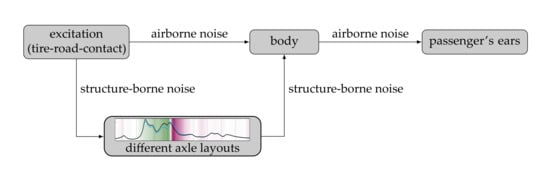
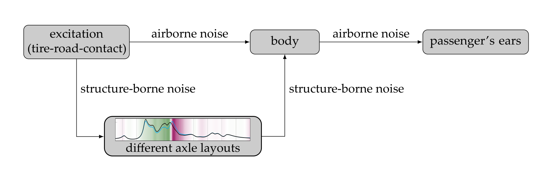
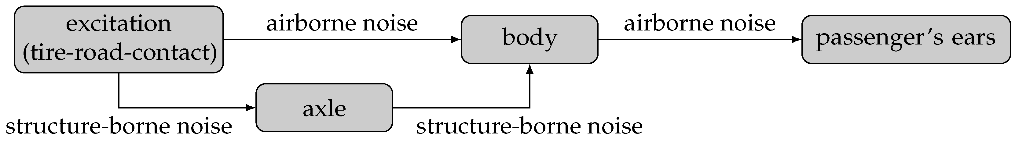
NVH—for noise, vibration, and harshness—describes the comfort of a vehicle for both acoustical and mechanical vibrations [5] (p. 208). The vehicle interior noise consists mainly of three components that are engine, wind, and road noise [9] (p. 3). Up to 300 Hz [9] (p. 235), road noise travels as structure-born noise from the contact patch between a tire and the road through the axle into the passenger cabin [3] (p. 19). The complete path is given in Figure 1. The axle transmits structure-borne noise from the wheel hub into the car body. One of the requirements to the axle is to reduce that transmitted noise. Additionally, it has to fulfill requirements from driving dynamics, safety, package, durability, weight, and cost [10] (p. 22).
1.2.1. Optimizing Road Noise
Road noise reduction results mainly from an optimization of the passive suspension parts such as bushings, which includes adjustments of the stiffness and the damping [11] (p. 1). The final adjustments of these bushings often take place in the late development process as they can be modified without package changes [2] (p. 55). Finding parameters for minimal noise transfer is challenging though, as there is a trade-off between NVH and handling, ride comfort, and durability [12] (p. 1).
One approach to solving this target conflict is the use of active systems, instead of optimizing passive suspensions [1] (p. 8). There are different types of active systems. Electric active suspension systems are able to reduce vibrations up to 5 Hz [13] (p. 45) by changing stiffness and damping of the suspension in order to optimize NVH and driving dynamics performance, depending on the current driving situation. Recent developments use piezo-electric subframe mounts to reduce structure-borne noise [14]. Active Noise Cancelling (ANC) systems reduce narrow bands like engine orders or broadband noise by the use of loudspeakers in the passenger compartment [15] (pp. 39–40). In particular, active systems with hardware actors seem to be exclusive for higher vehicle segments though [5,16].
The axle’s transfer path is not only determined by elasticity and damping, but also by mass, inertia, and the geometrical layout [17,18]. As the potentials of tweaking the elasticity and the damping of the bushings are well known, the kinematics of the suspension has an unknown effect on the transfer function [10] (p. 77).
1.2.2. Suspension Kinematics
Suspension kinematics need to ensure safe driving in all conditions, but it may also be possible to use them to optimize the NVH behavior of the vehicle at the same time. As suspension kinematics are generated early in the product development process, this could incorporate NVH development into the holistic development process. This matches Original Equipment Manufacturer’s (OEM’s) wish for earlier NVH development as described by Rambacher et al. [2] (p. 55). In literature, there are many different approaches to modify suspension kinematics, some of them also using these kinematics to improve NVH performance.
Niersmann inverts typical axle development processes and uses specified driving dynamic parameters to automatically generate suspension kinematics [19]. However, she does not investigate the effects on road noise. Schlecht investigates brake judder and vibrations caused by tire imbalances on the steering wheel and the seat rail [10]. He uses multi body simulation (MBS) to optimize suspension kinematics regarding haptic vibrations. An experimental vehicle developed by Vosteen can help to investigate the influences of kinematics on the comfort and dynamics behavior [20]. As this approach requires hardware, it is not applicable to early series development.
1.2.3. Automated FE Model Generation
To change the kinematics of the suspension, the geometries of the parts need to be modified. In the early development phases, this means changing simulation models and Finite Element (FE) parts. Those parts have to be remeshed [21] (p. 170) to predict the new axle behavior. Having many versions of suspension kinematics, this process cannot be carried out individually for each version. One method to avoid remeshing is part simplification. Fang and Tan develop twist beam axles by modeling them in FE as simplified beam elements [22]. Using this approach, an automated iterative design process becomes possible without remeshing parts by hand. However, this process can only be applied for geometrically simple parts, as complex parts cannot be simplified using beam elements.
2. Methods
Changing the suspension kinematics in the early development phase requires FE models to be rebuilt which includes generating new component FE models. Our method aims at simplifying and automating this process allowing two main goals. On the one hand, we want to predict NVH results from kinematics changes. On the other hand, we want to use the method to optimize suspension kinematics regarding NVH performance.
Our method uses the first available FE model of the axle under investigation and modifies it automatically in order to investigate kinematics influences on interior road noise. To fit existing models to new kinematics, we use two different approaches depending on the complexity of the changed parts. Simple parts like suspension links for instance are modeled in Section 2.2.1 using simplified geometries such as FE beam elements. Complex parts like the knuckle adapt to new kinematics by being morphed in Section 2.3.1. This method allows us to change the simulation model parametrically without knowing changes beforehand, as Helm et al. suggest [23] (p. 27). Additionally, we are not dependent on manual, time consuming, and fault-prone modeling of suspension kinematics as described by Niersmann [19] (p. 2).
The method is designed to determine NVH effects of shifting the kinematic hard points. In this paper, we demonstrate potential road noise improvements by investigating the effects of a displacement of one hard point in the axle layout. We move the connection point between the track rod and the knuckle by 10 mm against the driving direction in Section 3 and discuss the results in Section 4.
2.1. Simulation Model
In this paper, we investigate the rear axle of a front driven car. The complete transfer chain from excitation to the passenger’s ears is visualized in Figure 1. The excitation on the tire patch creates structure-borne vibrations that are transmitted through the tire and the wheel via the wheel hub into the axle. From there, the suspension’s links transmit them to the subframe attachment points as well as the damper and spring attachment points. The car body transmits them into the passenger cabin where the structure-borne noise becomes airborne noise.
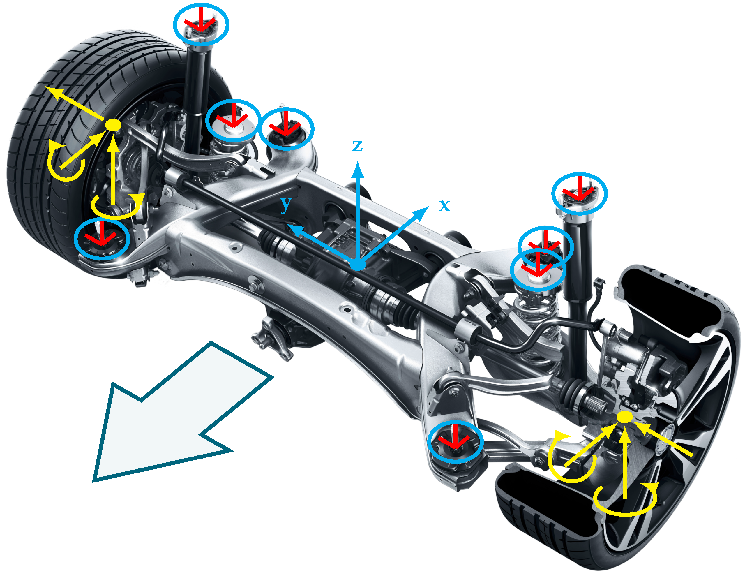
We investigate only the axle subsystem to identify potential modifications to reduce noise transfer through the axle. The FE simulation model consists of the complete axle from both wheel hubs to all the attachment points between axle and car body. We will use the coordinate system given in Figure 2. The axle in this figure differs from the axle under investigation. As the actual axle is still under development, no images of it can be shared. The coordinates’ origin lies in the center between both wheel hubs. With the driving direction indicated by the large arrow, the x-axis points backwards. The y-axis points to the right when looking in the driving direction and z to the top.
We calculate the Frequency Response Functions (FRF) that characterize the transfer behavior of the axle. We investigate the axle subsystem from the wheel hub to the car body connection points. The attachment points are fixed to the inertial system which is known as blocked force investigation [25] (p. 225). The simulation consists of 10 separate load cases. For each side, left and right, we excite the wheel hub with three translational force spectra and two torque spectra. In Figure 2, the yellow arrows mark force and torque excitations. The forces attack in x, y and z directions. The excitation amplitudes are 1 N for the complete spectrum from 1 Hz to 200 Hz. Torque is applied around the x- and z-axis at 1 Nm for the same spectrum. The torque in the y-direction would simply turn the wheel hub. As we do not consider friction in the wheel hub, there would be no excitation to the axle. Using these excitations, we calculate the transfer functions for the axle subsystem that can characterize the transmission of road disturbances that occur not only in the vertical direction [26] (p. 395).
For each of these 10 load cases, we get resulting forces at all the attachment points. In Figure 2, the blue circles highlight the eight attachment points: the spring and damper as well as the front and back of the subframe for both the left and the right part of the axle. For each of these eight points, we receive three force spectra—respectively in the x-, y- and z-directions—per load case. In Figure 2, the small red coordinate systems indicate these force spectra.
All mentioned calculations add up to
result spectra per simulation. In order to reduce complexity, we add up all the individual load case result spectra. For all eight attachment points i, we name the number of the load case and the result spectrum of this load case for example for the x-direction . We calculate the resulting spectrum for one attachment point and one resulting force direction by energetically adding up all j spectra
leaving 24 root mean square (RMS) spectra. This is done following van der Linden et al. [27] (p. 3) and Sell who recommends adding energetically for high frequencies [28] (p. 2). As we are analyzing up to 200 Hz and wanting to get transfer functions without preliminary phase assumptions, we decided to apply this method. It is possible to further reduce the number of spectra, as the left part of the axle is symmetrical to the right part. This omits 12 spectra leaving 12 force spectra for each simulation that represents energetically the added transfer functions from the wheel hub to each attachment point direction.
Using these transmitted forces, we are able to rate the axle’s transmission behavior directly by interpreting transferred forces into the car body. In order to optimize the sound pressure levels at the passenger seats, we can include the simulated axle subsystem back into the complete transfer path from Figure 1 to calculate interior road noise [2,27].
2.2. Modeling Parts for Changed Kinematics
Changing the kinematics implies modifying components of the suspension. Shifting the hard point between the knuckle and track rod requires the modification of these two parts and the relocation of the bushing. All the other parts stay unchanged.
The modification of FE parts is split into two steps. First, simple parts such as the track rod are automatically rebuilt from scratch fitting the new kinematics, as described in Section 2.2.1. Secondly, complex parts like the knuckle are automatically morphed as explained in Section 2.3.1 in a way they fit the new kinematics without corrupting unchanged connections. Morphing includes the disadvantage of changing the part’s stiffness, but, on the other hand, it is what happens when the geometry of a part is changed in reality. This problem is more thoroughly discussed by Schlecht [10] (p. 89). Elastomer bushings automatically rotate into the new kinematics. According to Fang and Tan and Schlecht, their properties remain the same, as stiffness and damping cannot be specified definitely in the early development phase [10,22].
2.2.1. Modifying the Track Rod
The track rod is a simple part of the suspension. It is a long, thin rod that connects two hinges mainly by tension or compression [5] (p. 550). The original part in Figure 3a is completely modeled using FE shell elements for the rod part, the bushing ring, and the bushing clamp. On the left, we display the back view—on the right, the top view. In the middle, the cross section is displayed. The track rod is hollow because it is made from a bent sheet metal. The FE model was created by meshing a Computer Aided Design (CAD) part in a preprocessor.
For the investigation of numerous kinematics variants, this process is too time-consuming. Therefore, we simplified the structure and automated its creation. The first simplification in Figure 3b, which we will call version 1, is to replace the shell meshed rod part in the middle of the track rod by FE beam elements. These elements describe a beam analytically [21] (p. 98). All of the input parameters are cross section locations and cross section dimensions. The bevel of the cross section is omitted. The amount of beam elements is determined by the bending mode needed to model the axle behavior. Additionally, we need individual beam sections to model changing cross sections. This requires more elements than the bending modes. The ring part and the clamp part are replaced by parametrically defined FE meshes. This way, we are able to create a complete track rod with some sampling points, dimensions for the cross section and dimensions for ring and clamp. This allows us to easily modify geometric parameters such as coordinates or cross sections.
The next simplification in Figure 3c, version 2 is to connect the ring and clamp by omitting all the sampling points. Errors introduced into the simulation by these simplifications will be investigated in Section 2.3. Our Python generator enables us to automatically create an array of simplified track rod variations to systematically identify significant geometric parameters which can be used for NVH optimization.
2.3. Validation of a Simplified Model
The effects resulting from the changes made to the track rod in Section 2.2.1 must be well known. Using that knowledge, we can assess whether changes in the transfer function result from model simplifications or kinematics changes. We investigate the simplified track rod on three levels. First, we check changes in the component properties itself. Then, we look at the eigenmodes of the complete axle using the original track rod as well as the simplified versions. Finally, we investigate changes in the FRFs resulting from simplifying the track rod.
The validation on a component level compares the original model (Figure 3a) with the simplified version 1 of the track rod (Figure 3b). Version 2 is not only a simplification but also a geometry change and therefore another component, which is why we investigate version 2 only in the complete axle and not on the component level.
The relative error for the mass of version 1 with respect to the original mass
is below 1%. The absolute error of the center of gravity differs by less than 0.5 mm in each direction x, y, and z.
The averaged relative error of the inertia in principal axes lies within 2%. The inertia of the rotation around the connection axis between both connection points is much smaller than the other two inertias. The relative error for the small inertia is greater than the other relative errors.
The next criterion to validate is the eigenmodes of the complete axle. We compare them using Modal Assurance Criterion (MAC) values. Using the eigenvectors of model 1 for mode number m and of model 2 for mode number n, the MAC value
calculates the orthogonality between both eigenvectors. Its values range from 0 to 1. Matching modes have higher MAC values. For example, 0.8 could be a threshold value [29] (p. 132).
Figure 4 shows the MAC plots for the complete axle using the original track rod and the simplified track rod version 2. Figure 4a shows the comparison, Figure 4b,c the auto MAC values for the original and version 2 model, respectively. For the auto MAC value, the same model is used twice in Equation (4). It is commonly used to identify similar looking modes. In the MAC plots, mode numbers start from 3 since modes 1 and 2 are the rigid body modes of the two break disks rotating around the wheel hub at 0 Hz.
Overall, Figure 4a shows no noticeable difference between the original and version 2 of the track rod up to mode 47 at 160 Hz. For modes 6 to 8, the auto MAC from Figure 4b,c indicates similar looking modes at different frequencies. For modes 48 and 49, there is a mode flip. This indicates a frequency shift of at least one of these two modes. Above mode 52 at 180 , MAC values decrease with mode 53 disappearing.
The MAC plots from Figure 4 don’t give any information regarding frequency shifts. We can only identify mode shifts if the frequencies of single modes are shifted so that the order of the modes changes. Therefore, we plot all the high MAC values next to the diagonal line in Figure 4a into a new Figure 5. We see the modes of the original model on the top line, the ones of version 1 on the middle line and version 2 on the baseline. Arrows indicate where mode frequencies lie for each model version using the MAC value colors from Figure 4. Straight arrows from top to bottom indicate no change in mode frequencies.
It seems clear that there is no change in mode frequencies up to 130 . For modes 38 and 39, the two track rods are bending in phase and in opposite phase respectively. The simplified version 1 shifts these two modes down by and version 2 up again with mode 39 ending in the same frequency as it was originally and mode 38 shifted down by 1 . For mode 48, there is a shift by 4 with no other shifts up to 180 . Above that, we see mode 53 disappearing in version 2 as already seen in Figure 4a.
After checking the component parameters and axle eigenmodes, we now investigate influences on the FRFs. We use the simulation model from Section 2.1 for the original model, simplified model version 1 and version 2.
Figure 6 shows FRF for all three models for the left attachment points. We see all three directions for the attachment points spring, damper, subframe front, and subframe rear. The color code in the background indicates relative differences between the original model and the simplified models. It indicates the maximum relative deviation from the original model, to either simplified model version 1 or 2. The scale of the color indicator from −30% to +30% will be relevant and discussed in Section 3. All three FRF lines are almost indistinguishable, which leads us to the conclusion that the simplification of the modeling as well as the geometry itself is possible without affecting the FRF function in a relevant way. The darker colors to the right indicate some larger relative deviations where the FRF values themselves are below 1. This results in bigger relative errors for minimal deviations. For frequencies above 200 , changes are even smaller.
2.3.1. Knuckle
The knuckle needs a different approach to fit the mesh to the new suspension kinematics. Because of the complex shape of the part, it is not possible to simplify it using beam elements as it was done for the track rod. Therefore, we use the existing mesh and morph it in order to fit the new kinematics.
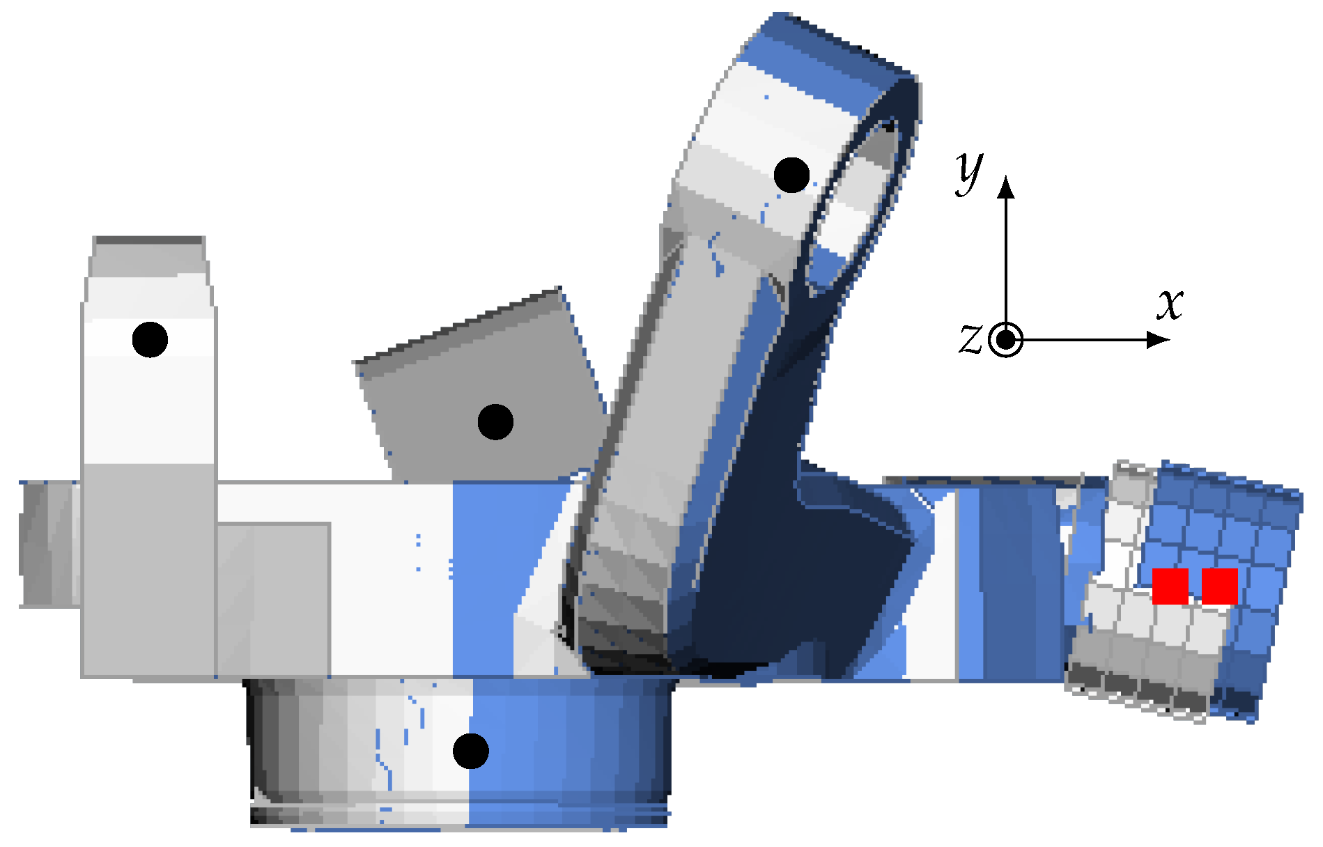
Each part of the suspension has got k specific connection points that either have to stay unchanged or follow an imposed displacement. The knuckle is connected to all suspension links including the track rod, the brake caliper, and the wheel bearing. For all these attachment points, we impose translations. This is represented in Figure 7 in the top view. In white, we see the original knuckle geometry. The black dots and red squares indicate some of the points that receive an imposed displacement. The red connection between the knuckle and the track rod is moved in the x-direction and all the other black points shall stay unchanged. This results in the blue part. Ideally, only the FE nodes near the shifted point will be moved.
In a first, and later omitted approach, we used Lagrange polynomials to interpolate directly onto FE nodes. The sum of all Lagrange polynomials in one point
which describes its displacement depending on all imposed displacements . The left part of the product is the basic Lagrange polynomial [30] (p. 188) expanded to three dimensions. Because of the function’s nonlinearity, small imposed displacements far away from the interpolation point could lead to huge displacements at the interpolation point. Even an additional factor considering the distance to the imposed points didn’t fulfill the requirements because of varying distances. Therefore, we omitted this approach.
Instead of Lagrange polynomials, using Discrete Sibson interpolation was found to be a working approach. We used the Python implementation by Stevens [31], which is released under MIT-License [32]. Discrete Sibson interpolation, also called natural neighbor interpolation, uses a three-dimensional Voronoi diagram that defines cells around each imposed point. A regular grid specifies points, where function values from the imposed points are interpolated. The overlapping area of a new Voronoi cell around the grid point with the already existing Voronoi cells is used as weighting factor. This method ensures that each grid point is only affected by given displacements adjacent to the said grid point [33].
Because the implementation by Stevens can only interpolate onto a regular grid, we need to attach a second interpolation. Using the displacement values on the regular grid, we can interpolate from the grid onto each individual FE node using Python’s RegularGridInterpolator library [34]. This function uses the regular grid data received from the Discrete Sibson interpolation and linearly interpolates the data onto each individual FE node.
We use this tool chain consisting of two separate interpolations three times, once for each translational direction x, y, and z. As we keep the original meshing and only shift FE nodes, we distort some of the FE elements. Because FE elements are sensitive towards distortion [21] (p. 307), this method is limited to small displacements. In the future, for bigger displacements, a remeshing procedure should be attached to the interpolation process in order to ensure sufficient element quality.
3. Results
Using the method described in Section 2, it is possible to automatically create FE simulation models for changed suspension kinematics. To demonstrate the possibilities of the method, we move the connection point between the knuckle and the track rod. The red squares in Figure 7 between the knuckle and the track rod indicate the backward shift in a positive x-direction by 10 mm. The original model in white is changed into the model in blue. The automatic morphing only shifts the connection point marked in red while all the black points stay unchanged. This increases the lever arm between the wheel hub and the track rod. Additionally, we automatically generate simplified straight beam track rods and assemble a new axle model. In this investigation, we always use the simplified straight track rod version 2 from Figure 3c, hence from now on simply naming it track rod.
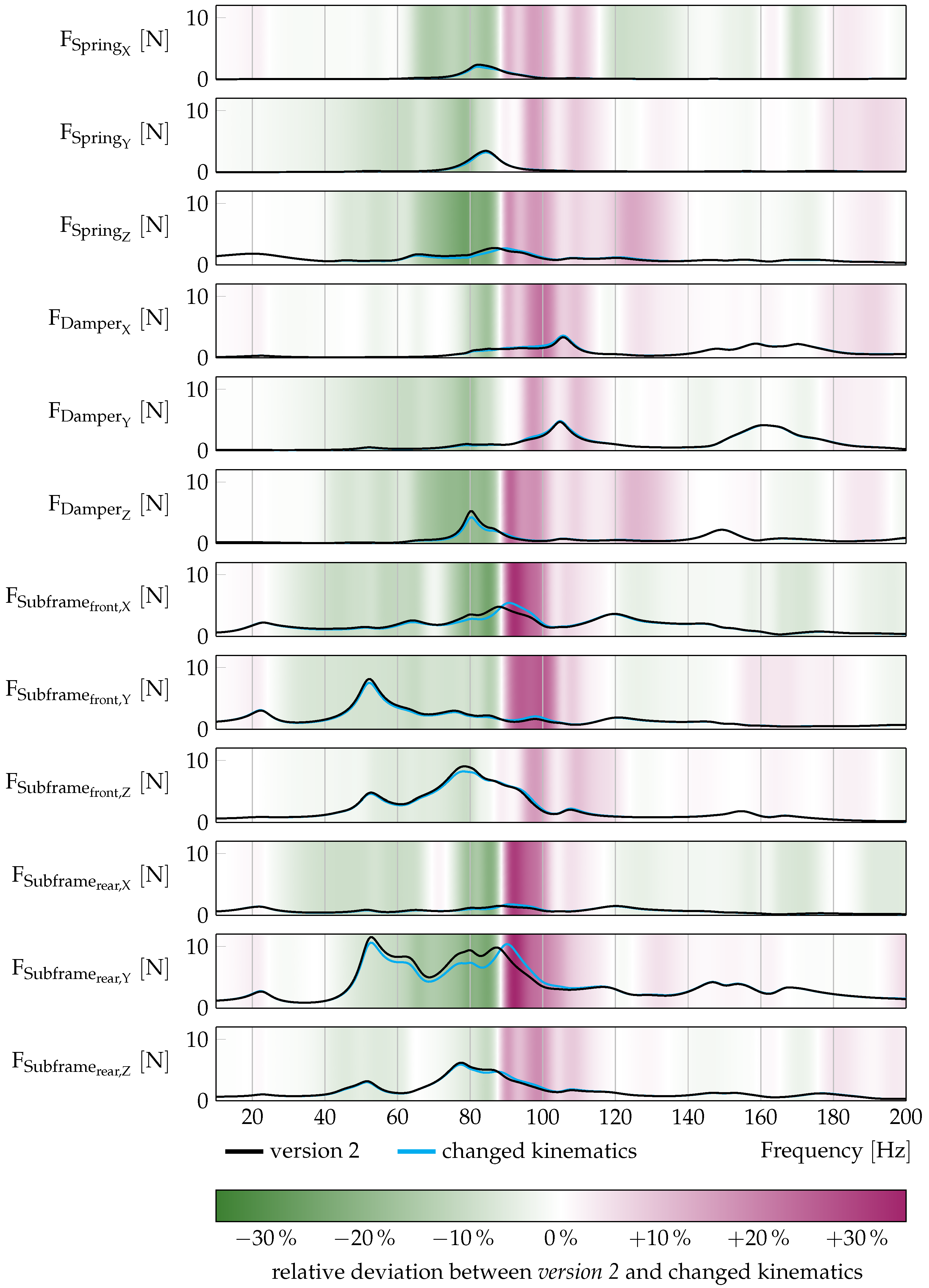
The resulting FRF curves are shown in Figure 8. In black, we see the FRF function of the original suspension kinematics. The blue line represents the changed kinematics using an artificially generated new track rod and a morphed knuckle.
The first thing to notice is the underlying color code representing the relative difference between both curves. Because it is the same scaling as in Figure 6, we immediately notice the increased difference. The maximum absolute differences between the modified and the original kinematics are four times larger than the differences between the original model and version 2. This leads us to the conclusion that kinematics changes are able to change transferred forces through the axle in the hearing frequency range.
For all attachment points, we are able to shift the peak transmitted force to a different frequency. Here, the peak is shifted from 87 Hz to 90 , indicated by an amplitude improvement for frequencies below 88 and an amplitude rise above this frequency. This phenomenon is further investigated in Section 4. If the transfer path from coupling points to airborne noise at the passenger’s ears is frequency dependent, a kinematics optimization reducing interior road noise may be feasible.
Especially for the rear subframe mount, we are able to change transferred forces in the y-direction. From 50 Hz to 88 , the level of transmitted force is reduced by up to 23.9%. This improvement is in contrast to an increase by up to 34.3% above 88 .
4. Discussion
In Figure 8, a distinct white line can clearly be observed between improvement and deterioration at 88 . We wish to discuss what is the underlying physical principle behind this prominent phenomenon.
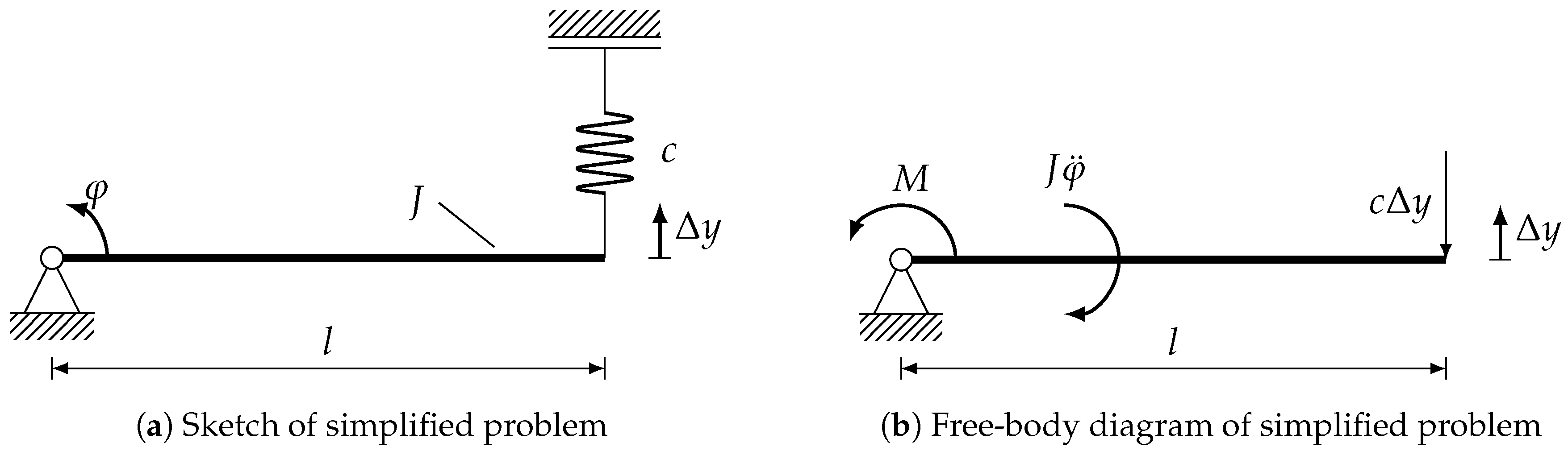
Changing the connection point between the knuckle and the track rod by moving it in a positive x-direction can be investigated by the simplified undamped model given in Figure 9a. We see the axle from the top with the wheel hub as the fixed mount with a rotational degree of freedom. This represents the steering rotation. The track rod and its connection to the knuckle and the subframe is modeled by a spring with stiffness c. The knuckle with inertia J rotates around the wheel hub in the coordinate . The length between the wheel hub and the connection point between the knuckle and the track rod is named l. If the knuckle rotates, the spring is compressed by but does not introduce any torque.
The free-body diagram is given in Figure 9b. An external torque is introduced around the wheel hub, symbolizing torques generated by lateral forces in the contact patch of the tire. Because of the caster, this force results in a torque around the wheel hub. The spring’s force can be linearized as
for small angles. From the free body diagram, we get the differential equation for the system
Solving the homogeneous part, we get the eigenfrequency
which indicates that increasing l also increases the eigenfrequency if we assume there is no change in stiffness and inertia.
Assume a harmonic excitation with excitation frequency and amplitude as
and the solution ansatz for the particular solution
We can get the amplification function
The absolute value results from ignoring phases as described in Section 2.1 on page 5.
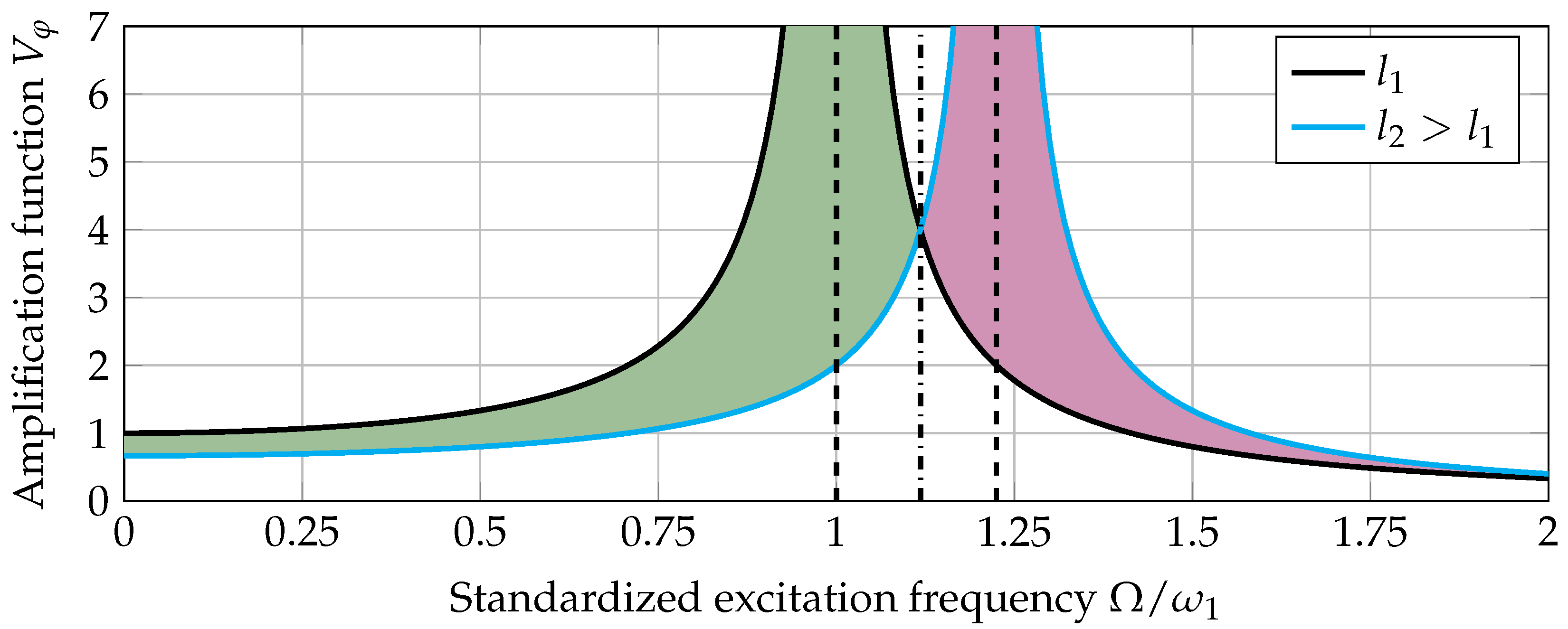
To investigate effects from increasing l, we compare for with .
Both amplification functions are given in Figure 10. We assumed that c and J were worth 1 in order to get simple plots. We can see the two poles at and indicated by two black dashed lines. They are calculated by Equation (8) and they are the zero of the denominator in Equation (11). Shifting the amplification function by enlarging l leads to decreased amplitudes, indicated in green, left of the intersection point between both amplification functions. To the right of it, amplitudes are increased, indicated in red. Calculating this intersection point by solving
for , we get
Using all this information, we are now able to investigate the white line at 88 from Figure 8. The green color on the left and red on the right indicate the effect illustrated in Figure 10. Knowing the reason, we can search for modes that were formerly below 88 and were shifted by the kinematics change above 88 . Their delta to 88 has to fulfill Equation (13).
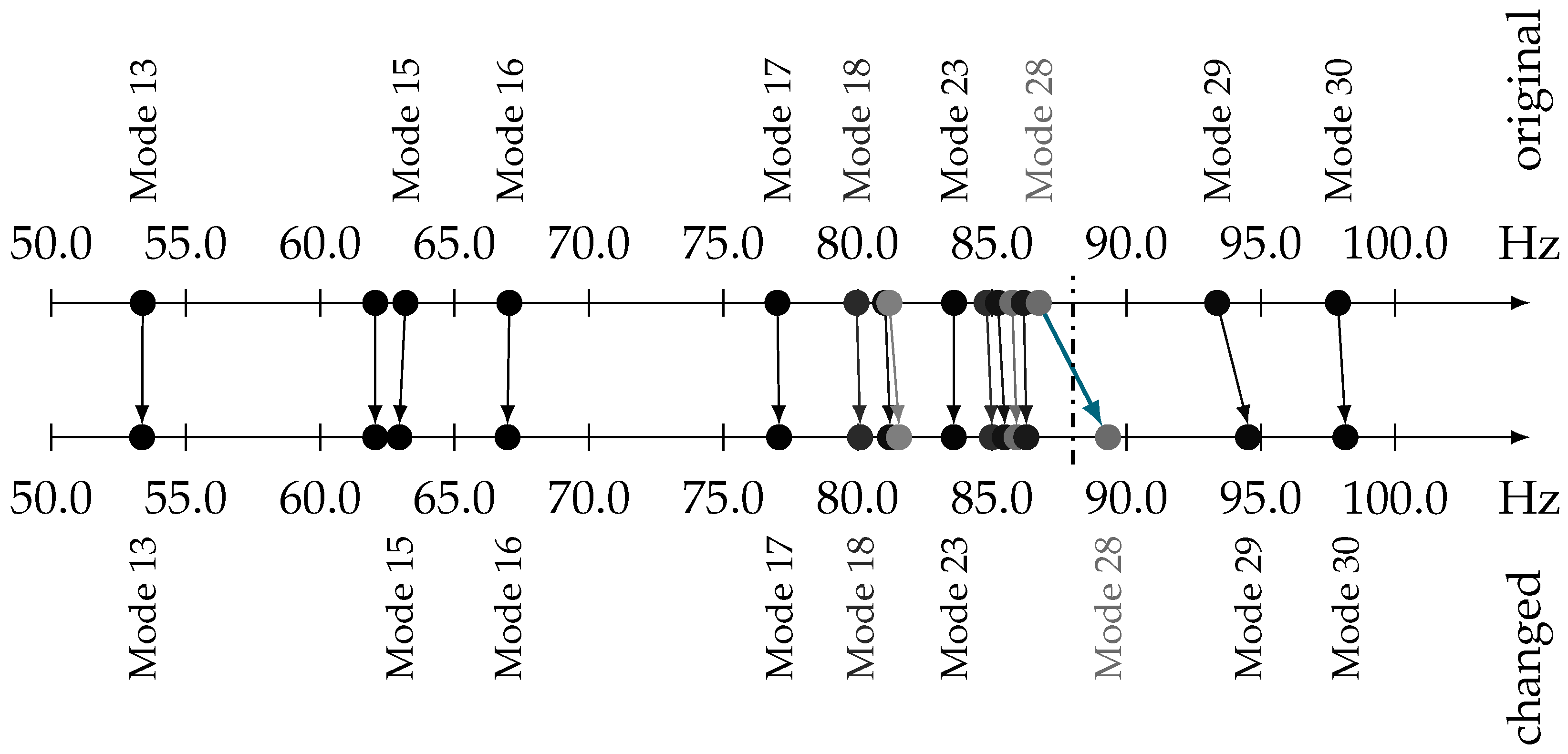
In Figure 11, we see modes from 50 Hz to 100 in the same MAC color code used in Figure 4. On the top line are the modes before changing the kinematics—on the bottom the modes after changing the kinematics. Straight arrows from top to bottom indicate no change in the mode’s frequencies. Diagonal arrows indicate a mode shift. We clearly see mode 28 being shifted from up to . Using Equation (13), we get a splitting frequency of . Additionally, we find the maxima of all changes in Figure 8, indicated by maximum green and red color exactly at both the old and new eigenfrequencies, respectively.
5. Conclusions
In this paper, we presented a method to investigate effects from suspension kinematics changes to the suspension transfer function in the hearing frequency range. We simplified FE suspension simulation models using beam elements to model the track rod and geometry morphing to adapt the knuckle to the new kinematics. This enables an automated simulation model generation. On the one hand, this allows us to automatically rate suspension kinematics changes regarding their influence on interior road noise, and, on the other hand, to optimize suspension layouts for better NVH performance. This includes optimization of suspension hard point coordinates as well as cross sections and paths of suspension links. Contrary to the modification of stiffness and damping parameters in suspension bushings, this introduces further possibilities to modify the suspension transfer path. These layout and design modifications can lead to better NVH performance independently from any additional system such as active suspensions with only the use of existing suspension parts.
In this paper, we showed the potential influence on interior road noise up to 200 by shifting the hard point between the knuckle and the track rod 10 mm to the back of the car. This shifts the steering eigenmode by and affects transferred forces by up to almost 35 %.
For future work, the simplification and morphing of suspension FE parts introduced in this paper could create a database for parametrically described parts like links, knuckles, and subframes. By getting rid of the limitation to small kinematics changes described in Section 2.3.1, this could be used to easily predict interior rolling noise for completely new axle concepts already in the concept phase. For further investigation, we will extend the method to include ratings for ride and handling to ensure plausible suspension kinematics modifications and layout suggestions. The simple generation of suspension FE simulation models could help identify NVH relevant suspension geometry parameters. These simplified models and identified parameters could be used for the design of actors in active suspensions to modify the suspension layout in new ways in order to optimize interior road noise.
Author Contributions
Conceptualization, T.v.W. and F.G.; Formal analysis, T.v.W.; Investigation, T.v.W.; Methodology, T.v.W. and J.C.; Project administration, T.v.W.; Software, T.v.W. and J.C.; Supervision, F.G.; Validation, T.v.W. and J.C.; Visualization, T.v.W.; Writing—original draft, T.v.W.; Writing—review and editing, J.C. and F.G. All authors have read and agreed to the published version of the manuscript.
Funding
This research received funding by Daimler AG.
Acknowledgments
The authors thank the Daimler AG with the department NVH road noise, especially Ernst Prescha, Stéphanie Anthoine, and Christoph Meier for their support. Additionally, the authors would like to thank the members from the team and department for always being available to discuss the ongoing research. The authors thank Achim Winandi from the Karlsruhe Institute of Technology for valuable input and support.
Conflicts of Interest
The authors declare no conflict of interest. Timo von Wysocki and Jason Chahkar are from Daimler AG, the company had no role in the design of the study; in the collection, analyses, or interpretation of data; in the writing of the manuscript, and in the decision to publish the results.
Abbreviations
The following abbreviations are used in this manuscript:
| ANC | Active Noise Cancelling |
| CAD | Computer Aided Design |
| FE | Finite Element |
| FRF | Frequency Response Function |
| MAC | Modal Assurance Criterion |
| MBS | Multi Body Simulation |
| NVH | Noise Vibration and Harshness |
| OEM | Original Equipment Manufacturer |
| RMS | Root Mean Square |
References
- Pfeffer, P.E. Die Komplexität kann man nicht reduzieren. ATZextra 2018, 23, 6–9. [Google Scholar] [CrossRef]
- Rambacher, C.; Ehrt, T.; Sell, H. Schwingungsoptimierung ganzer Achsen. Automob. Z. 2017, 119, 54–59. [Google Scholar] [CrossRef]
- Mantovani, M. Rollgeräusche kann man nicht mit Emotionen verbinden. Automob. Z. 2018, 120, 18–21. [Google Scholar] [CrossRef]
- Kim, J.K.; Lee, J.; Kim, H.G.; Cho, M.; Ih, K.D.; Ko, H.Y.; Shim, J.S. The Effects of Suspension Component Stiffness on the Road Noise: A Sensitivity Study and Optimization. In Proceedings of the 10th International Styrian Noise, Vibration & Harshness Congress, Graz, Austria, 20–22 June 2018; SAE Technical Paper Series; SAE International: Warrendale, PA, USA, 2018; pp. 1–7. [Google Scholar] [CrossRef]
- Ersoy, M.; Gies, S. (Eds.) Fahrwerkhandbuch: Grundlagen, Fahrdynamik, Komponenten, Systeme, Mechatronik, Perspektiven, 5th ed.; ATZ/MTZ-Fachbuch; Springer Vieweg: Wiesbaden, Germany, 2017. [Google Scholar] [CrossRef]
- Elbers, C.; Bäumer, B.; Siddiqui, S.; Albers, I. Entwicklung und Optimierung einer innovativen Verbundlenkerachse. Aachener Kolloquium für Fahrzeug- und Motorentechnik 2009, 18, 537–552. [Google Scholar]
- Botev, S. Digitale Gesamtfahrzeugabstimmung für Ride und Handling; Vol. 684, Fortschritt-Berichte VDI Reihe 12, Verkehrstechnik/Fahrzeugtechnik; VDI Verlag GmbH: Düsseldorf, Germany, 2008. [Google Scholar]
- Schilp, A.; Bathelt, H. NVH development strategies for suspensions—Challenges and chances by autonomous driving. In Proceedings of the Automotive Acoustics Conference; Siebenpfeiffer, W., Ed.; Springer Vieweg: Wiesbaden, Germany, 2017. [Google Scholar] [CrossRef]
- Zeller, P. (Ed.) Handbuch Fahrzeugakustik: Grundlagen, Auslegung, Berechnung, Versuch, 3rd ed.; ATZ/MTZ-Fachbuch; Springer Vieweg: Wiesbaden, Germany, 2018. [Google Scholar] [CrossRef]
- Schlecht, A. Minimierung der Schwingungsempfindlichkeit von Kraftfahrzeugvorderachsen. Ph.D. Thesis, Technische Universität München, München, Germany, 2012. [Google Scholar]
- Willenborg, D. Elastomer-Fahrwerkslager Simulativ Ausgelegt. Wie Beeinflusst Eine Geometrieänderung Die Federkonstante? Available online: https://automobilkonstruktion.industrie.de/fahrwerk/wie-beeinflusst-eine-geometrieaenderung-die-federkonstante/ (accessed on 8 August 2018).
- Kido, I.; Nakamura, A.; Hayashi, T.; Asai, M. Suspension Vibration Analysis for Road Noise Using Finite Element Model; SAE Technical Paper Series; SAE International: Warrendale, PA, USA, 1999. [Google Scholar] [CrossRef]
- Cytrynski, S.; Neerpasch, U.; Bellmann, R.; Danner, B. Das aktive Fahrwerk des neuen GLE von Mercedes-Benz. Automob. Z. 2018, 120, 42–45. [Google Scholar] [CrossRef]
- Gäbel, G.; Millitzer, J.; Atzrodt, H.; Herold, S.; Mohr, A. Development and Implementation of a Multi-Channel Active Control System for the Reduction of Road Induced Vehicle Interior Noise. Actuators 2018, 7, 52. [Google Scholar] [CrossRef] [Green Version]
- Zafeiropoulos, N.; Zollner, J.; Kandade Rajan, V. Aktive Dämpfung des Rollgeräuschs zur Verbesserung der Klangqualität im Fahrzeug. Automob. Z. 2018, 120, 38–43. [Google Scholar] [CrossRef]
- Schirle, T. Systementwurf eines elektromechanischen Fahrwerks für Megacitymobilität. Ph.D. Thesis, Karlsruher Institut für Technologie, Karlsruhe, Germany, 2019. [Google Scholar] [CrossRef]
- Troulis, M.; Gnadler, R.; Unrau, H.J. Übertragungsverhalten von Radaufhängungen für Personenwagen im komfortrelevanten Frequenzbereich. Automob. Z. 2004, 106, 336–348. [Google Scholar] [CrossRef]
- Chatillon, M.M.; Jezequel, L.; Coutant, P.; Baggio, P. Hierarchical optimization of the design parameters of a vehicle suspension system. Veh. Syst. Dyn. 2006, 44, 817–839. [Google Scholar] [CrossRef]
- Niersmann, A. Modellbasierte Fahrwerkauslegung und -Optimierung. Ph.D. Thesis, Technische Universität Braunschweig, Braunschweig, Germany, 2012. [Google Scholar]
- Vosteen, K. Ein Realtool zur Fahrwerkentwicklung. Aachener Kolloquium für Fahrzeug- und Motorentechnik 2008, 17, 1573–1591. [Google Scholar]
- Klein, B. FEM; Springer Fachmedien: Wiesbaden, Germany, 2015. [Google Scholar] [CrossRef]
- Fang, X.; Tan, K. Effiziente Konzeptauslegung von Verbundlenker-Hinterachsen. Automob. Z. 2015, 117, 42–47. [Google Scholar] [CrossRef]
- Helm, D.; Huf, A.; Zimmer, H.; Kondziella, R. Anforderungen in der Frühen Phase der Gesamtfahrzeugauslegung; VDI-Berichte 2169; VDI Verlag GmbH: Düsseldorf, Germany, 2012; pp. 21–40. [Google Scholar]
- Daimler Global Media. Mercedes-Benz C-Klasse T-Modell (S205) 2014, Raumlenker-Hinterachse: 14C577_03. Available online: https://media.daimler.com/marsMediaSite/de/instance/picture.xhtml?oid=7535355&ls=L3NlYXJjaHJlc3VsdC9zZWFyY2hyZXN1bHQueGh0bWw_c2VhcmNoU3RyaW5nPUQyMTIzMjkmc2VhcmNoSWQ9MiZzZWFyY2hUeXBlPWRldGFpbGVkJmJvcmRlcnM9dHJ1ZSZyZXN1bHRJbmZvVHlwZUlkPTE3MiZ2aWV3VHlwZT10aHVtYnMmc29ydERlZmluaXRpb249UFVCTElTSEVEX0FULTImdGh1bWJTY2FsZUluZGV4PTAmcm93Q291bnRzSW5kZXg9NQ!!&rs=0 (accessed on 28 August 2019).
- Van der Seijs, M.V.; de Klerk, D.; Rixen, D.J. General framework for transfer path analysis: History, theory and classification of techniques. Mech. Syst. Signal Process. 2016, 68-69, 217–244. [Google Scholar] [CrossRef]
- Zhu, J.J.; Khajepour, A.; Esmailzadeh, E.; Kasaiezadeh, A. Ride quality evaluation of a vehicle with a planar suspension system. Veh. Syst. Dyn. 2012, 50, 395–413. [Google Scholar] [CrossRef]
- Van der Linden, P.; van der Auweraer, H.; Wyckaert, K.; Hendricx, W. Noise and Vibration Transfer Path Analysis; Bus 2000; IMechE Conference Transactions; Professional Engineering for IMechE: Bury St Edmunds, UK, 2000; pp. 47–56. [Google Scholar]
- Sell, H. Geräuschpfadanalyse für Hochfrequenten Körperschall; Fortschritte der Akustik; Deutsche Gesellschaft für Akustik: Oldenburg, Germany, 2001. [Google Scholar]
- Rainieri, C.; Fabbrocino, G. Operational Modal Analysis of Civil Engineering Structures; Springer: New York, NY, USA, 2014. [Google Scholar] [CrossRef]
- Merziger, G.; Mühlbach, G.; Wille, D.; Wirth, T. Formeln + Hilfen höhere Mathematik, 8th ed.; Binomi-Verlag: Barsinghausen, Germany, 2018. [Google Scholar]
- Stevens, R. Discrete Sibson (Natural Neighbor) Interpolation: Naturalneighbor: 0.2.1. Available online: https://pypi.org/project/naturalneighbor/ (accessed on 19 August 2019).
- Open Source Initiative. The MIT License. Available online: https://opensource.org/licenses/MIT (accessed on 3 September 2019).
- Park, S.W.; Linsen, L.; Kreylos, O.; Owens, J.D.; Hamann, B. Discrete Sibson interpolation. IEEE Trans. Vis. Comput. Graph. 2006, 12, 243–253. [Google Scholar] [CrossRef] [PubMed]
- SciPy.org. Scipy.Interpolate.RegularGridInterpolator. Available online: https://docs.scipy.org/doc/scipy-0.16.1/reference/generated/scipy.interpolate.RegularGridInterpolator.html (accessed on 3 September 2019).
Figure 1.
Transfer chain for interior road noise from the excitation to the passenger’s ears, parts from [9] (p. 170).
Figure 1.
Transfer chain for interior road noise from the excitation to the passenger’s ears, parts from [9] (p. 170).

Figure 2.
Rear axle used to discuss the simulation model for this paper. Excitation in yellow, FRF at blue locations. Axle image by Daimler Global Media [24].
Figure 2.
Rear axle used to discuss the simulation model for this paper. Excitation in yellow, FRF at blue locations. Axle image by Daimler Global Media [24].

Figure 3.
Track rod drawings. Left: Back view, middle: Cross section, right: Top view.

Figure 4.
MAC plots comparing modes of original model m to modes of version 2 of simplified track rod model n for modes from 0 Hz to 200 Hz.
Figure 4.
MAC plots comparing modes of original model m to modes of version 2 of simplified track rod model n for modes from 0 Hz to 200 Hz.

Figure 5.
Mode shifts for different simplification versions from 0 Hz to 200 .

Figure 6.
FRF functions for the complete axle using the original track rod, simplified track rod version 1 and version 2.
Figure 6.
FRF functions for the complete axle using the original track rod, simplified track rod version 1 and version 2.

Figure 7.
Morphed knuckle for new suspension kinematics with the track rod connection on the right side. Original kinematics in white, changed kinematics in blue. Black points indicate fixed points, the red squares indicate imposed translations
Figure 7.
Morphed knuckle for new suspension kinematics with the track rod connection on the right side. Original kinematics in white, changed kinematics in blue. Black points indicate fixed points, the red squares indicate imposed translations

Figure 8.
Differences between transferred forces of the complete axle with track rod version 2 and changed kinematics—left vehicle side.
Figure 8.
Differences between transferred forces of the complete axle with track rod version 2 and changed kinematics—left vehicle side.

Figure 9.
Simplified model of knuckle and track rod.

Figure 10.
Amplification function for two different lengths .

Figure 11.
Modes with MAC values greater than 0.7 on the main diagonal.

© 2020 by the authors. Licensee MDPI, Basel, Switzerland. This article is an open access article distributed under the terms and conditions of the Creative Commons Attribution (CC BY) license (http://creativecommons.org/licenses/by/4.0/).
Share and Cite
MDPI and ACS Style
von Wysocki, T.; Chahkar, J.; Gauterin, F. Small Changes in Vehicle Suspension Layouts Could Reduce Interior Road Noise. Vehicles 2020, 2, 18-34. https://0-doi-org.brum.beds.ac.uk/10.3390/vehicles2010002
AMA Style
von Wysocki T, Chahkar J, Gauterin F. Small Changes in Vehicle Suspension Layouts Could Reduce Interior Road Noise. Vehicles. 2020; 2(1):18-34. https://0-doi-org.brum.beds.ac.uk/10.3390/vehicles2010002
Chicago/Turabian Stylevon Wysocki, Timo, Jason Chahkar, and Frank Gauterin. 2020. "Small Changes in Vehicle Suspension Layouts Could Reduce Interior Road Noise" Vehicles 2, no. 1: 18-34. https://0-doi-org.brum.beds.ac.uk/10.3390/vehicles2010002