
Control Landscape of Measurement-Assisted Transition Probability for a Three-Level Quantum System with Dynamical Symmetry

Department of Mathematical Methods for Quantum Technologies, Steklov Mathematical Institute of Russian Academy of Sciences, 8 Gubkina Str., Moscow 119991, Russia
*
Author to whom correspondence should be addressed.
Quantum Rep. 2023, 5(3), 526-545; https://0-doi-org.brum.beds.ac.uk/10.3390/quantum5030035
Submission received: 5 May 2023
/
Revised: 30 June 2023
/
Accepted: 4 July 2023
/
Published: 13 July 2023
Abstract
:Quantum systems with dynamical symmetries have conserved quantities that are preserved under coherent control. Therefore, such systems cannot be completely controlled by means of only coherent control. In particular, for such systems, the maximum transition probability between some pairs of states over all coherent controls can be less than one. However, incoherent control can break this dynamical symmetry and increase the maximum attainable transition probability. The simplest example of such a situation occurs in a three-level quantum system with dynamical symmetry, for which the maximum probability of transition between the ground and intermediate states using only coherent control is , whereas it is about using coherent control assisted by incoherent control implemented through the non-selective measurement of the ground state, as was previously analytically computed. In this work, we study and completely characterize all critical points of the kinematic quantum control landscape for this measurement-assisted transition probability, which is considered as a function of the kinematic control parameters (Euler angles). The measurement-driven control used in this work is different from both quantum feedback and Zeno-type control. We show that all critical points are global maxima, global minima, saddle points or second-order traps. For comparison, we study the transition probability between the ground and highest excited states, as well as the case when both these transition probabilities are assisted by incoherent control implemented through the measurement of the intermediate state.
1. Introduction
Quantum control attracts high interest due to fundamental reasons related to the ability to manipulate quantum systems and due to various existing and prospective applications in quantum technologies [1]. Coherent control is realized by lasers or an electromagnetic field [2,3,4]. Incoherent control can be realized by various forms of the environment. One particular form of incoherent control is control using the back-action of non-selective quantum measurements, either projective or continuous. The general formulation for assisting the coherent control of quantum systems using the back-action of non-selective quantum measurements was developed in [5]. Various incoherent control strategies using the back-action of quantum measurements have been applied to many problems, such as enhancing the controllability of systems with dynamical symmetry [6], developing incoherent control schemes for quantum systems with wavefunction-controllable subspaces [7], using measurements to enhance controllability [8], manipulating a qubit [9], incoherently controlling retinal isomerization in rhodopsin [10], controlling transitions in the Landau–Zener system [11], modifying the decay rates of excited states in open quantum systems [12], inducing Boolean dynamics for open quantum networks [13], steering quantum states by using the sequences of weak blind measurements [14], incoherently controlling a qubit using the quantum Zeno effect [15], applying decoherence-assisted optimal quantum state preparation [16], building quantum-feedback-like models of photosynthesis [17], controlling quantum state transfer based on the optimal measurement [18], etc. The energy-measurement-induced quantum damping of position for an atom bouncing on a reflecting surface in the presence of a homogeneous gravitational field was investigated [19]. The measurement-induced decoherence of trapped ions prepared in a nonclassical motional state was shown to inhibit the internal population dynamics and damp the vibrational motion [20]. The mapping of an unknown mixed quantum state onto a known pure state using the sequential measurements of two noncommuting observables only and without the use of unitary transformations was studied [21]. Zeno-type effects in a superconducting qubit in the presence of structured noise baths and variable measurement rates were used to suppress and accelerate qubit decay [22]. Quantum measurements were used to control weak values in the Cheshire Cat effect in open quantum systems [23]. A quantum clock driven by entropy reduction through measurement was proposed [24]. The Zeno effect was used to demonstrate universal control between non-interacting qubits [25] and generate a multi-qubit entangling Zeno gate [26]. A measurement-based estimator scheme for continuous quantum error correction was proposed [27]. Steering a two-level system using weak measurements in addition to the system Hamiltonian was shown to allow the targeting of any pure or mixed state [14]. Stroboscopic driving combined with repeated measurement-like interactions with an external spectator system was applied for optimal quantum state preparation [16]. A measurement-based feedback approach with reinforcement learning exploiting the non-linearity of weak measurements with coherent driving was proposed to prepare cavity Fock state superpositions [28]. Measurement-based control was applied to find the minimum energy eigenstate of a given energy function [29]. The control of two-level systems by using positive unital maps associated with quantum Lotka–Volterra operators was considered [30]. Projective quantum measurement induces the collapse of the wavefunction into the eigenstate of the observable that corresponds to the observed eigenvalue. Another paradigm is protective measurements, which are able to preserve the coherence of the quantum state during the measurement process and allows the extraction of the expectation value of an observable by measuring a single quantum system [31].
A typical quantum control problem is formulated as the maximization of some objective functional (fidelity) that represents the desired property of the system to be optimized. An important topic is the analysis of the dynamic and kinematic quantum control landscapes [32,33,34]. The dynamical control landscape is defined as a graph of the objective functional as a functional of the control. The kinematic control landscape is formed by representing the dynamics of the controlled quantum system by transformation maps (e.g., by unitary transformations or Kraus maps) instead of differential evolution equations and considering the parameters of these maps as controls.
Key points of the control landscape are global maxima (for maximization of the objective) and global minima (for minimization of the objective). Traps are local but not global maxima (resp., minima) of the control landscape. An important type of critical point is the second-order trap—a critical point where the Hessian of the objective is negative (resp., positive) semi-definite but not strictly negative (resp., positive). At such points, the objective may still grow (resp., decrease) along directions in the control space that correspond to zero eigenvalues of the Hessian, but the growth is slower than the second order of small variations in the control. Second-order traps were introduced and studied in [33] (see also [35]). The importance of the analysis of kinematic control landscapes was shown for closed systems in [32]. For open quantum systems, the analysis of the kinematic control landscape was performed in [36], and a unified analysis for both quantum and classical systems was performed in [37]. Applications to problems in chemistry were found [38,39].
Quantum systems with dynamical symmetries are of particular interest in quantum control [6,8,40,41,42]. Such systems are not completely controllable by means of coherent control, while they may have no Hermitian observables that are invariant under all controls (while for any particular control, such invariant observables may exist). Instead of that, they may have some different conservation laws. This symmetry can be broken using some kind of incoherent control, as was implemented, for example, using the back-action of non-selective quantum measurements in [6] for a three-level system with dynamical symmetry (see Figure 1). For this system, the maximum transition probability between the ground and intermediate states using only coherent control was shown to be [41]. In [6], the maximum transition probability when coherent control was assisted by the non-selective measurement of the population of the ground state was computed and shown to be . An important analysis of this system was performed in [8], where the following problem was considered and solved: find an observable such that its von Neumann measurement, along with coherent control, allows the initial state to be completely steered into a target state. In this case, the choice of the measured observable is considered as control according to [5].
In this work, we consider this three-level quantum system in more detail. We find and characterize all critical points of the transition probability , and in this sense, we completely describe its kinematic quantum control landscape, which we show consists of global maxima, global minima, saddle points and second-order traps. For comparison, we compute the maximum measurement-assisted transition probability between the ground and upper excited states, as well as the maxima of both these transition probabilities when assisted by the measurement of the intermediate state .
The structure of this work is the following. Section 2 reviews the general idea of control using the back-action of quantum measurements. In Section 3, we provide the formulation of the considered problem. Section 4 contains necessary results from spin-1 representation theory. Section 5 contains preliminary computations of the measurement-assisted transition probabilities in the kinematic representation of controls. Section 6 contains a detailed analysis of the kinematic control landscape for the transition probability . Section 7 contains the computation of the maximum values of the transition probability assisted by the measurement of state or and the transition probability assisted by the measurement of state . The Discussion section (Section 8) summarizes the results.
2. Measurement-Assisted Quantum Control
In this section, we discuss in detail the scheme of quantum control using the back-action of non-selective quantum measurements in the formula introduced in [5].
Measurements performed on a quantum system are generally probabilistic: measurement outcomes for identical measurements performed on identically prepared quantum systems vary and are obtained with certain probabilities. Another important difference between quantum measurements and measurements performed on classical systems is that measurements of quantum systems not only allow the extraction of some information about the system but also often change the state of the system, and such a state change can be significant.
Consider the non-selective measurement of a system observable (a Hermitian operator) with eigenvalues and spectral projectors , , . Eigenvalues are the possible measurement outcomes. If is the density matrix of the system before the measurement, then the measurement outcome is obtained with the probability . If the observer looks at the measurement apparatus and reads the measurement outcome , then the system state immediately after the measurement will be transformed to . This reduction is known as the collapse of the wavefunction. Non-selective measurement corresponds to a situation in which the <<observer>> does not look at the measurement apparatus and does not read the measurement outcome. The outcome for this situation can be described as the average of the realization of all possible measurement outcomes with their corresponding probabilities. In this situation, the measurement outcome is the average value , and according to the von Neumann–Lüders postulate [43,44], the non-selective measurement of the observable O transforms the density matrix as follows:
In particular, the non-selective measurement of a population of some state transforms the density matrix as follows:
where is the identity operator. In quantum control, quantum measurements can be used for real-time feedback, which was developed for models of quantum optics in [45,46,47]. In this scheme, some control (e.g., a shaped laser field) continuously acts on the controlled quantum system, and during this process, a discrete or continuous selective measurement of a certain observable is performed, and the measurement outcome is processed to modify the applied control in real time. Various achievements have been made in quantum feedback control. A coherent quantum feedback strategy was proposed [48]. The problem of quantum feedback control in the context of established formulations of classical control theory was discussed [49]. The Hamilton–Jacobi–Bellman equation for quantum optimal feedback control was derived [50]. The ability to simulate universal dynamical control through the repeated application of only two coherent control operations and a simple “Yes-No” measurement was shown [51]. To control the position and momentum of observables, the experimental measurement-based quantum control of the motion of a millimeter-sized membrane resonator was demonstrated [52]. An approach to information transfer in spintronics networks via the design of time-invariant feedback control laws without recourse to dynamic control was proposed [53]. Applications of quantum feedback to quantum engineering are discussed in the review in [54]. Measurement-based feedback cooling operating deep in the sideband-unresolved limit was demonstrated [55]. Feedback quantum control with deep reinforcement learning was applied to driving a system with double-well potential with high fidelity toward the ground state [56]. Feedback control was proposed for the control of a solid-state qubit [57], non-linear systems [58], quantum state manipulation [59], multi-qubit entanglement generation [60], the formation of coupled-qubit-based thermal machines [61], the steering of an energy function to the minimum energy eigenstate in variational quantum algorithms [29], etc.
Real-time feedback control can potentially be very powerful but is difficult to realize experimentally due to the need for fast real-time processing of the measurement outcome. However, since non-selective quantum measurements themselves modify the state of the system, they can potentially be used for control, even without feedback. Such a scheme has the advantage of not using fast real-time processing of the measurement outcome but at the cost of needing to measure various quantum observables. The mathematical formulation of using non-selective quantum measurements with or without coherent quantum control was developed in [5], where, apart from the general formulation, the two-level case was completely analytically solved: in this case, the optimal measured observables and the maximum attained fidelity for maximizing the transition probability in a two-level quantum system by using any given number of non-selective measurements were analytically computed. The general formulation includes coherent or incoherent control during time intervals , inducing the CPTP dynamical map in each interval and non-selective measurements of observables at time moments . The overall evolution of the initial density matrix will be
The control goal is to optimize, in addition to coherent and incoherent controls, the measured observables to maximize a given control objective (e.g., to realize an optimal state transfer).
Another view on this type of quantum control can be described via the famous Zeno and anti-Zeno effects. The quantum Zeno effect, predicted by L. Khalfin [62,63] and B. Misra and E. C. G. Sudarshan [64], states that making continuous non-selective measurements of the population of some state of a quantum system, which has its own internal evolution, leads to the freezing of the system in the measured state, independent of the internal system evolution. It is reminiscent of the arrow paradox (aporia) of the Greek philosopher Zeno of Elea, where, for an observation of a flying arrow at any one (duration-less) instant of time, the arrow is neither moving to where it is, nor to where it is not. Then, it is concluded that, since at every instant of time, there is no motion occurring, if the arrow is motionless at every instant and if time is entirely composed of instants, then the motion of the arrow would be impossible. In the quantum anti-Zeno (or dynamical Zeno) effect [65], one performs a non-selective measurement of some time-dependent state of the quantum system, which evolves with its internal dynamics. As a result, in the limit of continuous measurements, independently of the internal dynamics, the system will follow the time-dependent state of the measured observable, so the system density matrix at time t will be . The anti-Zeno effect can be used to control the quantum system if one considers the time-dependent measured observable to be the control. If , then the non-selective measurement of via anti-Zeno dynamics transfers the system to the target state , thereby realizing the state transfer of the system. The complete realization of such a state transfer can be performed in the limit of the continuous measurement of the observable , which can be difficult to perform. Therefore, a natural question is how to produce the best approximation of the anti-Zeno dynamics by using a fixed number N of quantum measurements. For the two-level case, such an optimal approximation of the anti-Zeno effect using N quantum measurements was found [5]. The maximum transition probability was computed to be
where is the angle between Bloch vectors of the initial and target states. The anti-Zeno effect is obtained in the limit of an infinite number of measurements when the interval between any two consecutive measurements tends to zero, .
Thus, in this work, the scheme of control using the back-action of non-selective measurements based on [5] is different from both quantum feedback control and Zeno-type control. It is different from feedback since it does not read the measurement outcome. It is different from Zeno-type control since it uses a finite number of measurements. These differences lead to advantages and disadvantages. The advantages include the simpler experimental realization, since there is no need for real-time feedback and no need for continuous measurements. The potential disadvantage is the lower efficiency of control. How significant this decrease in efficiency is, of course, depends on the particular control problem and the sufficient level of fidelity that one needs to obtain.
3. Formulation of the Problem
We consider a three-level quantum system with dynamical symmetry, with the free and interaction Hamiltonians defined as (we set the Planck constant )
The energy level structure of this system is shown in Figure 1. Without loss of generality, one can set . Physically, such a Hamiltonian represents a three-level system whose interaction with the laser field consists of a dipolar interaction, with constant dipolar terms coupling only neighboring states, and is equivalent to a spin-1 particle, which was studied in [40]. The coherent dynamics of more general spin-like quantum systems was studied in [66]. The controllability of such a system was studied in [41], where it was shown that, such a system is not completely controllable by only coherent control. As mentioned above, the maximum transition probability for coherent control assisted by a single von Neumann measurement of the population of the ground state for this system is [6]. In [8], the problem of finding an observable such that its von Neumann measurement along with coherent control allows the complete steering of the initial state into a target state was solved.
The unitary evolution operator of this system evolving under the action of a coherent control satisfies the Schrödinger equation:
where is a identity matrix. The time-evolved pure state of this system can be written as
The coefficients in this expansion satisfy the normalization condition .
While this system is not controllable, it has no Hermitian observable that is conserved by all controls, i.e., there is no Hermitian observable O such that for any f, (if such an observable existed, its average value would be determined by the initial state and could not be modified by any control). Indeed, this condition can be satisfied for any f only if , which holds only for , as can be directly checked. For any particular control f, an invariant operator exists, as was shown in [67], where such an operator was even explicitly constructed; however, this invariant operator depends on f. Instead of the absence of an f-independent conserved Hermitian operator, it is known [41] that this system has the conservation law
Note that the quantity under the modulus in this constraint is also conserved. This conservation law, as was shown in [41], limits the maximum transition probability from state to state over all coherent controls f to
The transition probability is computed as for a large enough T, where the coefficients satisfy the initial condition , .
Consider now the non-selective measurement of a system observable O (a Hermitian operator) with spectral projectors . If is the density matrix of the system before the measurement, then the non-selective measurement of O transforms the density according to Equation (1). In particular, the non-selective measurement of a population of some state transforms the density matrix according to Equation (2).
Suppose that the quantum system (4) evolves under the action of a coherent control during the time interval with some sufficiently long time ; then, at , the non-selective measurement of the population of some state is performed, and finally, during the time interval with , the system again evolves under the action of some coherent control . Here, is the minimal time during which all allowed unitary evolutions can be generated. Then, its final density matrix at will be
In particular, the probabilities of transitions from state to state and from state to state when the measurement of the population of either or is performed are defined by setting in (7):
where and . Numerically constructed kinematic control landscapes are plotted in Figure 2. Below, we perform a theoretical analysis of these control landscapes.
4. Spin-1 Representation Theory
Since we are studying the kinematic control landscape of a system under two coherent controls, we need to consider the manifold
Now, we describe the parameterization of .
For this system, the free and interaction Hamiltonians generate a spin-1 representation of the Lie algebra . Let , and be standard generators of the spin-1 representation of the Lie algebra with matrices
which are written in the eigenbasis of denoted by , where the first value denotes spin, and the second value denotes spin projection. Below, we use the notation .
In the kinematic representation, we consider the allowed evolution operators given by Wigner’s D-matrices, which are parameterized by Euler angles [68,69].
The first parameterization that we use is
which we call parameterization. It is defined for . For , one has
so different pairs of and with the same determine one unitary operator [70]. The subset
has to be parameterized in another way.
The second parameterization is
which we call parameterization. It is determined for and has the same degeneracy for .
The two matrix exponents appearing in both parameterizations have the form
5. Transition Probabilities Driven by Coherent Control Assisted by One Non-Selective Measurement
Coherent controls and are called dynamic controls. The dynamic control landscape is defined as a graph of the transition probability , considered as a functional of coherent controls and . For the control landscape analysis, it is convenient to consider coherent controls as elements of the space so that the transition probability becomes a functional (not necessarily a surjection).
Kinematic controls are parameters determining allowed unitary evolutions, which are elements of . Below, we consider the transition probabilities as functions of the kinematic controls, as in [6]. In the kinematic representation, the system during the first period of evolution evolves with some unitary evolution operator , defined by Equation (5) with , and then one performs a non-selective measurement (we consider the measurement of the population of either state or ), and finally, after the measurement, the system evolves with another evolution operator , defined by Equation (5) with .
The transition probabilities in the kinematic representation, i.e., as functions on , become
Below, we consider and . We mainly concentrate on the most non-trivial case, i.e., , , for which we study the kinematic landscape in detail. For comparison, in Section 7, we also compute the maximum transition probabilities for the cases and numerically plot some of the corresponding control landscapes.
The initial system state (before the application of coherent control ) is . The first control transforms the initial state into
Consider the case . After performing the non-selective measurement of , the system density matrix will be
Finally,
Consider the case . After performing the non-selective measurement of , the system density matrix will be
Finally,
6. Kinematic Quantum Control Landscape of the Transition Probability
The kinematic control landscape is a function on , and from Equation (14), we know that the kinematic landscape of the transition probability is
Since we consider the three-dimensional representation of the Lie group, we choose Euler angle parameterization (see Section 4) to study the kinematic control landscape. The parameters in the unitary evolution operator (17) are called kinematic controls. We denote for . Thus, the transition probability is considered as a function of the kinematic control parameters on the corresponding open charts.
First, we consider parameterization to find critical points on . From (11) and (12), we obtain the following matrix representation of the evolution operator:
Using (17), we obtain
where , and is the control landscape function. Hence, the transition probability is a function of only three kinematic parameters: and .
The domain of the graph is . For , the kinematic landscape of the transition probability is shown in Figure 2. As mentioned in the Introduction, in [6], it was shown that
Lemma 1.
All critical points of , their types and the corresponding values of the function are given in Table 1.
Proof.
Let us find critical points of the function on the domain . The derivatives of are:
For later analysis, we will need the Hessian of :
We search for all the points where the gradient of is zero, i.e., . From the condition , we determine that such extreme points should lie on the surfaces:
Consider these cases separately.
- (1)
- . In this case,Thus, from the conditions , we find the critical points . The Hessian has the formOne has . Computing Hessian eigenvalues allows us to conclude that these are saddle points.
- (2)
- .In this case,which is equivalent toDividing the second equation by the first, we obtainfrom which we can express in terms of asWe notice that (which means that ) satisfies (19) for .Let us express from the second equation in (19):Using the trigonometric identitywe obtain the following equation for x:(We also need to consider and to make sure that we have not lost any solutions. From the system in (19), we notice that these two cases are not solutions for any ).Equation (20) can be solved analytically. Finally, we haveFinding from this equation, combined with the results obtained previously, we obtain the following critical points (which could be either extrema or saddle points):The corresponding values of the objective function areWe compute the second derivatives to determine the type of each of these critical points:(Only non-zero derivatives are written.) The Hessian matrix at the corresponding points isFrom Sylvester’s criterion, we conclude that
- (3)
- .All the critical points are easily found from (21):In the same way as for the case , we compute the second derivative to determine type of each of the critical points:The Hessian matrix at the corresponding points isFrom Sylvester’s criterion, we conclude that
□
Next, consider parameterization of the first coherent evolution and of the second coherent evolution to find the critical points on . Likewise, we obtain a matrix representation of unitary evolution, from which the transition probability will be
where . Our set corresponds to .
Lemma 2.
All critical points of on the surface , their types and the corresponding values of the function are given in Table 2.
Proof.
Thus, from the condition , we have the following critical points . The Hessian matrix at the corresponding points is
Since the eigenvalues are , we conclude that is a second-order trap. □
Next, consider parameterization of the second coherent evolution and of the first coherent evolution to find the critical points on . Likewise, we obtain a matrix representation of unitary evolution, from which the transition probability will be
where . The set corresponds to .
Lemma 3.
There are no critical points of on the surface .
Proof.
Thus, from the condition , we see that there are no critical points on the considered domain. □
Finally, consider parameterization of both the first and second coherent evolutions to find the critical points on . We will not provide the expression for in this parameterization, since we are only interested in the critical points and functional values on the surface (corresponding to ).
Lemma 4.
All critical points of on the surface , their types and the corresponding values of the function are given in Table 3.
Proof.
One can easily notice that , so are critical points for every .
The Hessian matrix at the corresponding points is
Its eigenvalues are . Since , points are global minima for every . □
It remains for us to study , , . Obviously, is a global minimum with , and determines the same functional as , i.e. .
Consider . We use representation to parameterize this set. The objective function has the following form:
where . From the simplicity of , the following lemma obviously follows.
Lemma 5.
All critical points of , their types and the corresponding values of the function are given in Table 4.
Consider . We use representation to parameterize this set. The objective function has the following form:
Lemma 6.
All critical points of on the surface and corresponding values are given in Table 5.
Proof.
Since , points are critical for every . The Hessian matrix at the corresponding points is
From Sylvester’s criterion, we conclude that is a second-order trap. □
Remark 1.
The types of critical points of are the same as for , , , , , (Table 6).
Theorem 1.
All the critical points of the kinematic control landscape of the transition probability are global minima, saddles, second-order traps or global maxima.
7. Comparison with other Cases of Measurement-Assisted Transition Probabilities
Here, for comparison, we study other cases of transition probabilities.
Theorem 2.
One has
Proof.
Here, there is no need to compute explicitly using Euler parameterization. Notice that
Since we can set (second evolution is trivial) and, after measurement, we have , we obtain
Similarly, we obtain
□
Theorem 3.
One has
Proof.
From (15), we obtain
Computing the transition probability gives
In this case, the transition probability is a function of only two kinematic controls, and . Notice that and . Thus,
□
8. Discussion
In this work, we considered a three-level quantum system with dynamical symmetry that is controlled by using coherent control assisted by the back-action of the non-selective quantum measurement of the population of some state. In the absence of the measurement, only of the population can be transferred from the ground to the intermediate state. Maximum measurement-assisted transition from the ground to the intermediate state was computed before. In the kinematic representation of the dynamics, the controls are Euler angles parameterizing the spin-1 representation of the Lie algebra . We studied in detail the kinematic control landscape of the transition probability from the ground to the intermediate state, describing all its critical points. We find that all critical points of the kinematic control landscape are global maxima, global minima, second-order traps or saddles. For comparison, we studied the transition probability between the ground and highest excited states, as well as the case when both these transition probabilities are assisted by incoherent control implemented through the measurement of the intermediate state. The next important question is what types of critical points are present in the dynamic control landscape. Let be the mapping that maps any control into the corresponding evolution operator with some fixed, sufficiently large T. Let be the kinematic transition probability (defined by Equation (16)). The dynamic landscape represents the transition probability as a function of two coherent controls, and (defined by Equation (8)), and can be considered as a composition of the mappings and as . At so-called regular points, where the Jacobian of the map from the control space to has full rank, the structure of the dynamical control landscape is the same as the structure of the kinematic control landscape (see Theorem 1 in [71]). Thus, our finding implies that at regular points, the dynamic landscape has the same points as the kinematic landscape. However, at singular points, where the Jacobian is rank-deficient, the situation can be different. Thus, our results do not exclude the existence of other critical points in the dynamic landscape as well. Finding such points and establishing the control landscape structure around them is an important problem that requires a special analysis beyond this work.
Author Contributions
Conceptualization, A.P.; methodology, A.P. and M.E.; formal analysis, M.E.; writing, A.P. and M.E.; visualization, M.E.; supervision, A.P.; discussion, A.P. All authors have read and agreed to the published version of the manuscript.
Funding
This work is supported by the Russian Science Foundation under grant № 22-11-00330, https://rscf.ru/en/project/22-11-00330/ (accessed on 5 May 2023) and was performed at Steklov Mathematical Institute of Russian Academy of Sciences.
Data Availability Statement
Not applicable.
Acknowledgments
We thank B.O. Volkov, V.N. Petruhanov and S.A. Kuznetsov for useful comments.
Conflicts of Interest
The authors declare no conflict of interest.
References
- Koch, C.; Boscain, U.; Calarco, T.; Dirr, G.; Filipp, S.; Glaser, S.; Kosloff, R.; Montangero, S.; Schulte-Herbrüggen, T.; Sugny, D.; et al. Quantum optimal control in quantum technologies. Strategic report on current status, visions and goals for research in Europe. EPJ Quantum Technol. 2022, 9, 19. [Google Scholar] [CrossRef]
- Rice, S.; Zhao, M. Modern Quantum Mechanics; John Wiley & Sons, Inc.: New York, NY, USA, 2000. [Google Scholar]
- Tannor, D. Introduction to Quantum Mechanics: A Time-Dependent Perspective; Univ. Science Books: Sausilito, CA, USA, 2007. [Google Scholar]
- Shapiro, M.; Brumer, P. Quantum Control of Molecular Processes. Second, Revised and Enlarged Edition; WILEY-VCH Verlag GmbH & Co. KGaA: Weinheim, Germany, 2012. [Google Scholar]
- Pechen, A.; Il’in, N.; Shuang, F.; Rabitz, H. Quantum control by von Neumann measurements. Phys. Rev. A 2006, 74, 052102. [Google Scholar] [CrossRef] [Green Version]
- Shuang, F.; Zhou, M.; Pechen, A.; Wu, R.; Shir, O.; Rabitz, H. Control of quantum dynamics by optimized measurements. Phys. Rev. A 2008, 78, 063422. [Google Scholar] [CrossRef]
- Dong, D.Y.; Chen, C.L.; Tarn, T.J.; Pechen, A.; Rabitz, H. Incoherent control of quantum systems with wavefunction controllable subspaces via quantum reinforcement learning. IEEE Trans. Syst. Man Cybern. Part Cybern. 2008, 38, 957–962. [Google Scholar] [CrossRef]
- Sugny, D.; Kontz, C. Optimal control of a three-level quantum system by laser fields plus von Neumann measurements. Phys. Rev. A 2008, 77, 063420. [Google Scholar] [CrossRef]
- Blok, M.; Bonato, C.; Markham, M.; Twitchen, D.; Dobrovitski, V.; Hanson, R. Manipulating a qubit through the backaction of sequential partial measurements and real-time feedback. Nat. Phys. 2014, 10, 189–193. [Google Scholar] [CrossRef] [Green Version]
- Lucas, F.; Hornberger, K. Incoherent control of the retinal isomerization in rhodopsin. Phys. Rev. Lett. 2014, 113, 058301. [Google Scholar] [CrossRef] [Green Version]
- Pechen, A.N.; Trushechkin, A.S. Measurement-assisted Landau-Zener transitions. Phys. Rev. A 2015, 91, 052316. [Google Scholar] [CrossRef] [Green Version]
- Zhang, P.; Ai, Q.; Li, Y.; Xu, D.; Sun, C. Dynamics of quantum Zeno and anti-Zeno effects in an open system. Sci. China Phys. Mech. Astron. 2014, 57, 194–207. [Google Scholar] [CrossRef] [Green Version]
- Qi, H.; Mu, B.; Petersen, I.R.; Shi, G. Measurement-induced boolean dynamics for open quantum networks. IEEE Trans. Control. Netw. Syst. 2023, 10, 134–146. [Google Scholar] [CrossRef]
- Kumar, P.; Snizhko, K.; Gefen, Y.; Rosenow, B. Optimized steering: Quantum state engineering and exceptional points. Phys. Rev. A 2022, 105, L010203. [Google Scholar] [CrossRef]
- Hacohen-Gourgy, S.; García-Pintos, L.P.; Martin, L.S.; Dressel, J.; Siddiqi, I. Incoherent qubit control using the quantum Zeno effect. Phys. Rev. Lett. 2018, 120, 020505. [Google Scholar] [CrossRef] [PubMed] [Green Version]
- Cejnar, P.; Stránský, P.; Střeleček, J.; Matus, F. Decoherence-assisted quantum driving. Phys. Rev. A 2023, 107, L030603. [Google Scholar] [CrossRef]
- Kozyrev, S.V.; Pechen, A.N. Quantum feedback control in quantum photosynthesis. Phys. Rev. A 2022, 106, 032218. [Google Scholar] [CrossRef]
- Harraz, S.; Yang, J.; Li, K.; Cong, S. Quantum state transfer control based on the optimal measurement. Optim. Control. Appl. Methods 2017, 38, 744–753. [Google Scholar] [CrossRef]
- Onofrio, R.; Viola, L. Quantum damping of position due to energy measurements. Phys. Rev. A 1996, 53, 3773–3780. [Google Scholar] [CrossRef] [Green Version]
- Viola, L.; Onofrio, R. Measured quantum dynamics of a trapped ion. Phys. Rev. A 1997, 55, R3291–R3294. [Google Scholar] [CrossRef] [Green Version]
- Roa, L.; Delgado, A.; Ladrón De Guevara, M.L.; Klimov, A.B. Measurement-driven quantum evolution. Phys. Rev. A 2006, 73, 012322. [Google Scholar] [CrossRef] [Green Version]
- Harrington, P.M.; Monroe, J.T.; Murch, K.W. Quantum Zeno effects from measurement controlled qubit-bath interactions. Phys. Rev. Lett. 2017, 118, 240401. [Google Scholar] [CrossRef] [Green Version]
- Dajka, J. Scattering–like control of the Cheshire Cat effect in open quantum systems. Quantum Rep. 2019, 2, 1–11. [Google Scholar] [CrossRef] [Green Version]
- Gangat, A.A.; Milburn, G.J. Quantum clocks driven by measurement. arXiv 2021. [Google Scholar] [CrossRef]
- Blumenthal, E.; Mor, C.; Diringer, A.A.; Martin, L.S.; Lewalle, P.; Burgarth, D.; Whaley, K.B.; Hacohen-Gourgy, S. Demonstration of universal control between non-interacting qubits using the quantum Zeno effect. NPJ Quantum Inf. 2022, 8, 88. [Google Scholar] [CrossRef]
- Lewalle, P.; Martin, L.S.; Flurin, E.; Zhang, S.; Blumenthal, E.; Hacohen-Gourgy, S.; Burgarth, D.; Whaley, K.B. A Multi-qubit quantum gate using the Zeno effect. arXiv 2022. [Google Scholar] [CrossRef]
- Borah, S.; Sarma, B.; Kewming, M.; Quijandría, F.; Milburn, G.J.; Twamley, J. Measurement-based estimator scheme for continuous quantum error correction. Phys. Rev. Res. 2022, 4, 033207. [Google Scholar] [CrossRef]
- Perret, A.; Bérubé-Lauzière, Y. Preparation of cavity Fock state superpositions by reinforcement learning exploiting measurement back-action. arXiv 2023. [Google Scholar] [CrossRef]
- Clausen, H.G.; Rahman, S.A.; Karabacak, Ö.; Wisniewski, R. Measurement-based control for minimizing energy functions in quantum systems. arXiv 2023. [Google Scholar] [CrossRef]
- Mukhamedov, F.; Qaralleh, I. Controlling problem within a class of two-level positive maps. Symmetry 2022, 14, 2280. [Google Scholar] [CrossRef]
- Piacentini, F.; Avella, A.; Rebufello, E.; Lussana, R.; Villa, F.; Tosi, A.; Gramegna, M.; Brida, G.; Cohen, E.; Vaidman, L.; et al. Determining the quantum expectation value by measuring a single photon. Nat. Phys. 2017, 13, 1191–1194. [Google Scholar] [CrossRef] [Green Version]
- Rabitz, H.A.; Hsieh, M.M.; Rosenthal, C.M. Quantum optimally controlled transition landscapes. Science 2004, 303, 1998–2001. [Google Scholar] [CrossRef]
- Pechen, A.N.; Tannor, D.J. Are there traps in quantum control landscapes? Phys. Rev. Lett. 2011, 106, 120402. [Google Scholar] [CrossRef] [Green Version]
- de Fouquieres, P.; Schirmer, S.G. A closer look at quantum control landscapes and their implication for control optimization. Infin. Dimens. Anal. Quant. Probab. Rel. Top. 2013, 16, 1350021. [Google Scholar] [CrossRef] [Green Version]
- Volkov, B.; Pechen, A. High-order traps in quantum control problems for certain strongly degenerate systems. Uspekhi Mat. Nauk. 2023, 78, 191–192. [Google Scholar] [CrossRef]
- Pechen, A.; Brif, C.; Wu, R.; Chakrabarti, R.; Rabitz, H. General unifying features of controlled quantum phenomena. Phys. Rev. A 2010, 82, 030101. [Google Scholar] [CrossRef] [Green Version]
- Pechen, A.; Rabitz, H. Unified analysis of terminal-time control in classical and quantum systems. Europhys. Lett. 2010, 91, 60005. [Google Scholar] [CrossRef] [Green Version]
- Moore, K.W.; Pechen, A.; Feng, X.J.; Dominy, J.; Beltrani, V.; Rabitz, H. Universal characteristics of chemical synthesis and property optimization. Chem. Sci. 2011, 2, 417–424. [Google Scholar] [CrossRef]
- Moore, K.W.; Pechen, A.; Feng, X.J.; Dominy, J.; Beltrani, V.J.; Rabitz, H. Why is chemical synthesis and property optimization easier than expected? Phys. Chem. Chem. Phys. 2011, 13, 10048–10070. [Google Scholar] [CrossRef]
- Hioe, F.T. Dynamic symmetries in quantum electronics. Phys. Rev. A 1983, 28, 879–886. [Google Scholar] [CrossRef]
- Turinici, G.; Rabitz, H. Quantum wavefunction controllability. Chem. Phys. 2001, 267, 1–9. [Google Scholar] [CrossRef] [Green Version]
- Engelhardt, G.; Cao, J. Dynamical symmetries of periodically-driven quantum systems and their spectroscopic signatures. Phys. Rev. Lett. 2020, 126, 090601. [Google Scholar] [CrossRef]
- Lüders, G. Über die Zustandsänderung durch den Meßprozeß. Ann. Phys. 2006, 8, 322. [Google Scholar] [CrossRef]
- von Neumann, J. Mathematical Foundations of Quantum Mechanics; Princeton University Press: Princeton, NJ, USA, 1955. [Google Scholar]
- Wiseman, H.W.; Milburn, G.J. Quantum Measurement and Control; Cambridge University Press: Cambridge, UK, 2014. [Google Scholar] [CrossRef] [Green Version]
- Wiseman, H.M.; Milburn, G.J. Quantum theory of optical feedback via homodyne detection. Phys. Rev. Lett. 1993, 70, 548–551. [Google Scholar] [CrossRef] [Green Version]
- Wiseman, H.M. Quantum theory of continuous feedback. Phys. Rev. A 1994, 49, 2133–2150. [Google Scholar] [CrossRef] [PubMed] [Green Version]
- Lloyd, S. Coherent quantum feedback. Phys. Rev. A 2000, 62, 022108. [Google Scholar] [CrossRef]
- Doherty, A.C.; Habib, S.; Jacobs, K.; Mabuchi, H.; Tan, S.M. Quantum feedback control and classical control theory. Phys. Rev. A 2000, 62, 012105. [Google Scholar] [CrossRef] [Green Version]
- Gough, J.; Belavkin V., P.; Smolyanov, O.G. Hamilton–Jacobi–Bellman equations for quantum optimal feedback control. J. Opt. B Quantum Semiclass. Opt. 2005, 7, S237–S244. [Google Scholar] [CrossRef]
- Lloyd, S.; Viola, L. Engineering quantum dynamics. Phys. Rev. A 2001, 65, 010101. [Google Scholar] [CrossRef]
- Rossi, M.; Mason, D.; Chen, J.; Tsaturyan, Y.; Schliesser, A. Measurement-based quantum control of mechanical motion. Nature 2018, 563, 53–58. [Google Scholar] [CrossRef] [Green Version]
- Schirmer, S.G.; Jonckheere, E.A.; Langbein, F.C. Design of feedback control laws for information transfer in spintronics networks. IEEE Trans. Automat. Contr. 2018, 63, 2523–2536. [Google Scholar] [CrossRef] [Green Version]
- Gough, J. Principles and applications of quantum control engineering. Phil. Trans. R. Soc. A. 2012, 370, 5241. [Google Scholar] [CrossRef]
- Guo, J.; Chang, J.; Yao, X.; Gröblacher, S. Active-feedback quantum control of an integrated, low-frequency mechanical resonator. arXiv 2023. [Google Scholar] [CrossRef]
- Borah, S.; Sarma, B.; Kewming, M.; Milburn, G.J.; Twamley, J. Measurement-based feedback quantum control with deep reinforcement learning for a double-well nonlinear potential. Phys. Rev. Lett. 2021, 127, 190403. [Google Scholar] [CrossRef]
- Ruskov, R.; Korotkov, A.N. Quantum feedback control of a solid-state qubit. Phys. Rev. B 2002, 66, 041401. [Google Scholar] [CrossRef] [Green Version]
- Jacobs, K.; Lund, A.P. Feedback control of nonlinear quantum systems: A rule of thumb. Phys. Rev. Lett. 2007, 99, 020501. [Google Scholar] [CrossRef] [Green Version]
- Fu, S.; Shi, G.; Proutiere, A.; James, M.R. Feedback policies for measurement-based quantum state manipulation. Phys. Rev. A 2014, 90, 062328. [Google Scholar] [CrossRef]
- Zhang, S.; Martin, L.S.; Whaley, K.B. Locally optimal measurement-based quantum feedback with application to multiqubit entanglement generation. Phys. Rev. A 2020, 102, 062418. [Google Scholar] [CrossRef]
- Bhandari, B.; Czupryniak, R.; Erdman, P.A.; Jordan, A.N. Measurement-based quantum thermal machines with feedback. Control Entropy 2023, 25, 204. [Google Scholar] [CrossRef] [PubMed]
- Khalfin, L.A. On the theory of decay at quasi-stationary state. Sov. Phys. Dokl. 1958, 2, 232. [Google Scholar]
- Khalfin, L.A. Contribution to the decay theory of a quasistationary state. Sov. Phys. JETP 1958, 6, 1053. [Google Scholar]
- Misra, B.; Sudarshan, E.C.G. The Zeno’s paradox in quantum theory. J. Math. Phys. 1977, 18, 756–763. [Google Scholar] [CrossRef] [Green Version]
- Balachandran, A.P.; Roy, S.M. Quantum anti-Zeno paradox. Phys. Rev. Lett. 2000, 84, 4019–4022. [Google Scholar] [CrossRef] [Green Version]
- Cook, R.J.; Shore, B.W. Coherent dynamics of N-level atoms and molecules. III. An analytically soluble periodic case. Phys. Rev. A 1979, 20, 539–544. [Google Scholar] [CrossRef]
- Lai, Y.-Z.; Liang, J.-Q.; Müller-Kirsten, H.J.W.; Zhou, J.-G. Time-dependent quantum systems and the invariant Hermitian operator. Phys. Rev. A 1996, 53, 3691–3693. [Google Scholar] [CrossRef] [PubMed]
- Wigner, E.P. Theory and its Application to the Quantum Mechanics of Atomic Spectra [Gruppentheorie und ihre Anwendungen auf die Quantenmechanik der Atomspektren]; Braunschweig: Vieweg Verlag, 1951; Griffin, J.J., Translator; Elsevier: Amsterdam, The Netherlands, 1959. [Google Scholar]
- Sakurai, J.J. Modern Quantum Mechanics; Cambridge University Press: Los Angeles, CA, USA, 1985. [Google Scholar]
- Kuprov, I. Spin: From Basic Symmetries to Quantum Optimal Control; Springer: Berlin/Heidelberg, Germany, 2023. [Google Scholar] [CrossRef]
- Wu, R.; Pechen, A.; Rabitz, H.; Hsieh, M.; Tsou, B. Control landscapes for observable preparation with open quantum systems. J. Math. Phys. 2008, 49, 022108. [Google Scholar] [CrossRef] [Green Version]
Figure 1.
Energy level structure and allowed transitions between the energy levels of a three-level quantum system with dynamical symmetry. The maximum transition probability using only coherent control is .
Figure 1.
Energy level structure and allowed transitions between the energy levels of a three-level quantum system with dynamical symmetry. The maximum transition probability using only coherent control is .

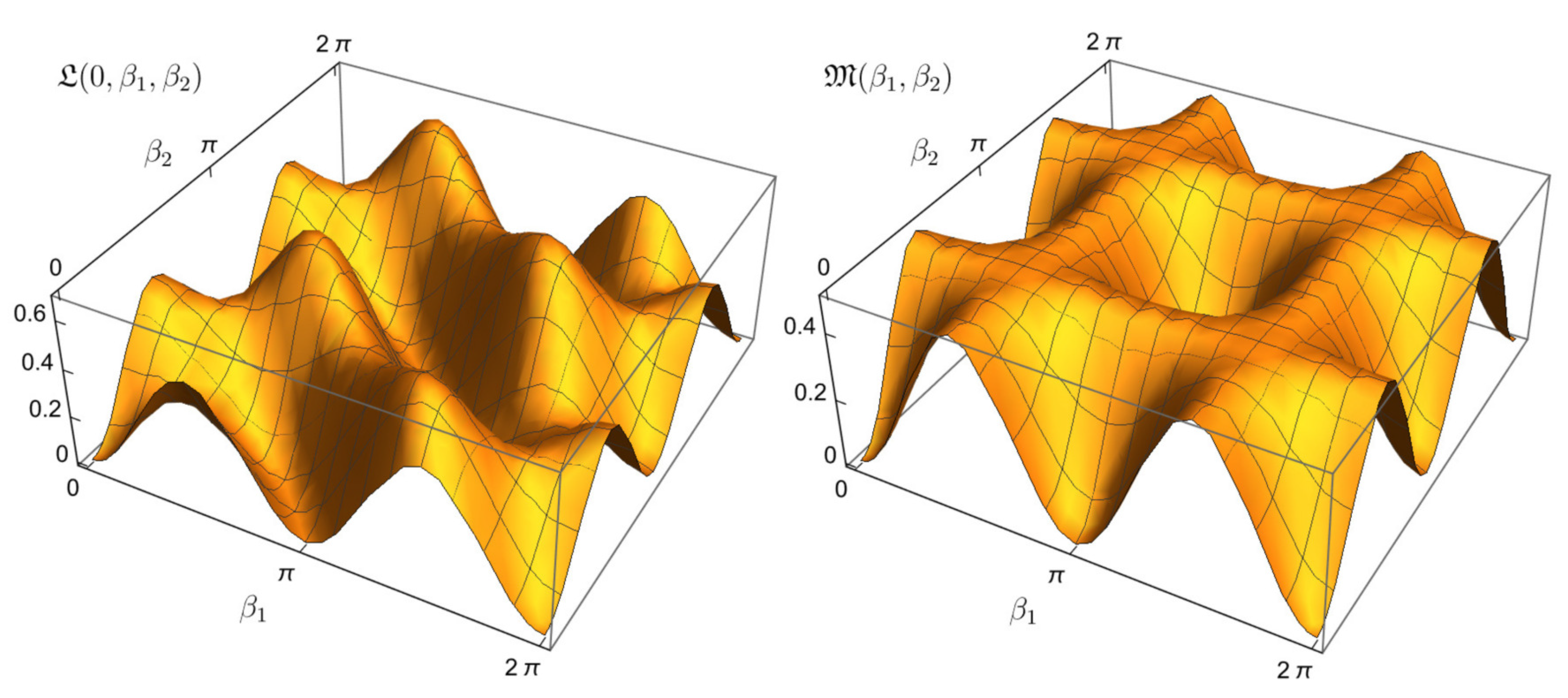
Figure 2.
Kinematic control landscapes of the transition probability . (Left): and (i.e., plot of the function ; see below). (Right): (i.e., plot of the function ; see below). The left landscape has second-order traps (see Theorem 1), whereas the right landscape is completely trap-free (see Theorem 3).


Table 1.
Critical points, their types and values of the objective function .
| Type of Point | ||
|---|---|---|
| Saddle point | ||
| , | Saddle point | |
| , | Saddle point | |
| , | Global maximum |
Table 2.
Critical points, their types and values of the objective function .
| Type of Point | ||
|---|---|---|
| , , | Second-order trap |
Table 3.
Critical points, their types and values of the objective function .
| Type of Point | ||
|---|---|---|
| , | 0 | Global minima |
Table 4.
Critical points, their types and values of the objective function .
| Type of Point | ||
|---|---|---|
| Second-order trap |
Table 5.
Critical points, their types and values of the objective function .
| Type of Point | ||
|---|---|---|
| , | Second-order trap |
Table 6.
Critical points, their types and values of the objective function. Asterisk indicates that the corresponding variable can take any value in its range.
Table 6.
Critical points, their types and values of the objective function. Asterisk indicates that the corresponding variable can take any value in its range.
| Type of Point | ||
|---|---|---|
| 0 | Global minima | |
| 0 | Global minima | |
| Saddle point | ||
| Saddle point | ||
| Saddle point | ||
| Saddle point | ||
| Saddle point | ||
| Second-order trap | ||
| Second-order trap | ||
| Second-order trap | ||
| Second-order trap | ||
| Second-order trap | ||
| Global maxima | ||
| Global maxima |
Disclaimer/Publisher’s Note: The statements, opinions and data contained in all publications are solely those of the individual author(s) and contributor(s) and not of MDPI and/or the editor(s). MDPI and/or the editor(s) disclaim responsibility for any injury to people or property resulting from any ideas, methods, instructions or products referred to in the content. |
© 2023 by the authors. Licensee MDPI, Basel, Switzerland. This article is an open access article distributed under the terms and conditions of the Creative Commons Attribution (CC BY) license (https://creativecommons.org/licenses/by/4.0/).
Share and Cite
MDPI and ACS Style
Elovenkova, M.; Pechen, A. Control Landscape of Measurement-Assisted Transition Probability for a Three-Level Quantum System with Dynamical Symmetry. Quantum Rep. 2023, 5, 526-545. https://0-doi-org.brum.beds.ac.uk/10.3390/quantum5030035
AMA Style
Elovenkova M, Pechen A. Control Landscape of Measurement-Assisted Transition Probability for a Three-Level Quantum System with Dynamical Symmetry. Quantum Reports. 2023; 5(3):526-545. https://0-doi-org.brum.beds.ac.uk/10.3390/quantum5030035
Chicago/Turabian StyleElovenkova, Maria, and Alexander Pechen. 2023. "Control Landscape of Measurement-Assisted Transition Probability for a Three-Level Quantum System with Dynamical Symmetry" Quantum Reports 5, no. 3: 526-545. https://0-doi-org.brum.beds.ac.uk/10.3390/quantum5030035