
Optical Dromions for Spatiotemporal Fractional Nonlinear System in Quantum Mechanics

1
School of Mathematics, South China University of Technology, Guangzhou 510640, China
2
Department of Basic Sciences and Related Studies, Mehran UET Shaheed Zulfiqar Ali Bhutto Campus Khairpur Mir’s, Khairpur 66020, Pakistan
3
Department of Mathematics, Lahore Campus, COMSATS University Islamabad, Lahore 54000, Pakistan
*
Author to whom correspondence should be addressed.
Quantum Rep. 2023, 5(3), 546-564; https://0-doi-org.brum.beds.ac.uk/10.3390/quantum5030036
Submission received: 1 April 2023
/
Revised: 21 May 2023
/
Accepted: 31 May 2023
/
Published: 18 July 2023
Abstract
:In physics, mathematics, and other disciplines, new integrable equations have been found using the P-test. Novel insights and discoveries in several domains have resulted from this. Whether a solution is oscillatory, decaying, or expanding exponentially can be observed by using the AEM approach. In this work, we examined the integrability of the triple nonlinear fractional Schrödinger equation (TNFSE) via the Painlevé test (P-test) and a number of optical solitary wave solutions such as bright dromions (solitons), hyperbolic, singular, periodic, domain wall, doubly periodic, trigonometric, dark singular, plane-wave solution, combined optical solitons, rational solutions, etc., via the auxiliary equation mapping (AEM) technique. In mathematical physics and in engineering sciences, this equation plays a very important role. Moreover, the graphical representation (3D, 2D, and contour) of the obtained optical solitary-wave solutions will facilitate the understanding of the physical phenomenon of this system. The computational work and conclusions indicate that the suggested approaches are efficient and productive.
1. Introduction
Currently, researchers are paying close attention to fractional calculus and its implications [1,2,3,4,5]. Fractional differential equations have been used to analyse a wide range of fractal systems [6,7,8]. Nonlinear fractional partial derivative equations (FPDEs) have many uses in the nonlinear sciences, including for electromagnetic radiation, electrolytic polarisation, visco-elasticity, optical fibres, control theory, data processing, quantum mechanics, astrophysics, switches, as well as biogenetics [9,10,11,12]. It has been noticed that FPDEs play an important role in dealing with and modelling nonlinear equations with applications in complex analysis [13]. Due to their importance as complex mathematical tools for the analysis and modelling of many biological and physical phenomena, fractional operators of various types have been used in the natural and scientific fields. FPDEs are a generalization of integer-order time–space partial differential equations that provide a concise representation of nonlinear systems. The Caputo–Riemann terminology [14], Fabrizio–Caputo description [15], Atangana–Baleanu–Caputo concept [16], and Grunwald–Letnikov interpretation [17] are by far the most extensively used fractional operator definitions, The major applications of these soliton solutions are in optics and photonics, including in the production of ultrafast laser pulses and the development of optical instruments for particle manipulation.
Many researchers in various scientific and technical fields pay more attention to dynamic systems described by FPDE today [18]. To study soliton solutions of FPDEs, various effective and productive methodologies have been explored in the literature and, as a result, sophisticated mathematical methods based on computer software are used to control these problems. Various authors systematically studied numerous experimental and analytical methods to achieve accurate travelling waves, quantitative and approximate solutions of all these models, such as the homotopy perturbation approach, the variational iteration method, the variable separation algorithm, and many more [19,20,21].
Due to the widespread use of FPDEs in engineering and science, the analysis of exact solutions of the nonlinear fractional Schrödinger equation (NFSE) has grown to the point where it is becoming a major source of concern around the world. Nonrelativistic quantum mechanical behaviour is explained by NFSEs, which are fundamental quantum physics models [22]. In 1965, Feynman et al. [23] observed path integrals over Brownian trajectories to construct the standard NFSE. Following that, new path integrals of Levy trajectories were substituted for Brownian trajectories, resulting in the NFSE [24]. Later, Laskin [25] formulated the space–time NFSE by using the quantum Riesz fractional approach. Since then, the NFSE has attracted the attention of a number of authors; for instance, Naber [26] considered the temporal NFSE under the Caputo fractional derivative. Muslih et al. [27] examined the time-NFSE as well as its solution employed in the Caputo sense. Eid et al. proposed an innovative NFSE model that included a nonsingular kernel, the fractional Caputo–Fabrizio concept, and the newer fractional Mittag–Leffler function operator. Smady et al. [22] explained the periodic and approximate solitary solutions of the NFSE employing the method of conformable residual series [28]. Guo et al. [29] used a class of energy procedures to test for the occurrence and uniqueness of the temporal NFSE solution. Naber [26] solved the NFSE for the first time in 2004. Furthermore, Jumarie [30] modified the fractional definition of the Riemann–Liouville derivative (RLD) by specifying a limit on the fractional difference to avoid the difficulties associated with deriving the constant fractionally. Many phenomena, as well as the non-Markovian evolution of a free molecule in elementary particle physics, fractional dynamics in quantum systems, the fractional Planck quantum energy ratio, etc., are described using the NFSE [31,32,33]. The TNFSE equation is rich and complex, and it can be utilized for mathematical analysis. Its solutions can display a variety of behaviours, including as soliton propagation, wave packet spreading, and chaotic dynamics. The study of the equation can lead to new ideas and developments in mathematics and physics.
Let us consider the following triple NFSE [34]:
where r and q are the real function of temporal t and spatial x variables, and where is a real constant with , and p is a complex one. and are, respectively, the modified RLD of functional orders “” and “” in term of “x” and “t”. Despite their significance, figuring accurate and consistent solutions to these nonlinear fractional models is incredibly difficult. It is a fundamental model of quantum mechanics that is used to model many exciting complex and nonlinear physical mechanisms, including photonics, harmonic oscillator, quantum condensates, fluid mechanics, shallow water waves, etc. The NFSE is used to characterize the Heisenberg dynamical model, which was created to evaluate what is consistent with quantum mechanics, as well as the Lagrange system, which is further consistent with classical physics. The aim of this study was to investigate optical solitons, bright, dark, coupled, trigonometric, rational, and hyperbolic solutions by using an AEM approach, as well as the integrability via the P-test approach. The P-test has been significant in the advancement of mathematical physics. It has been used for a wide range of physics topics, including the study of solitons, nonlinear waves, and quantum field theory. Moreover, the AEM approach is fundamental in the realm of differential equations and has played an important role in the advancement of modern mathematics and science.
This manuscript is organised as follows: We examine the P-test method in Section 2. The P-test approach is implemented in detail in Section 3 to examine the integrability of the governing system. The AEM scheme is explained in Section 4. In Section 5, the AEM technique is used to achieve an optical soliton solution. The results are presented in Section 6, and Section 7 covers the conclusion.
Definition
The crucial definition and parameters of Jumarie’s modification of the RLD are presented here, which are highly useful for presenting this work in a systematic manner. let be a continuous function. The modified RLD of order is then provided as follows:
Now, let be differentiable function at a point and be differentiable and defined in the range of “g”. Then,
- If = , then = for .
- = .
- = = .
In the following, if has a modified RLD of order , then it is called differentiable.
2. Painlevé Test (P-Test)
Generally, the P-test is employed to predict the integrability of NLSEs [35,36]. Ablowitz et al. [37] proposed the P-test for examining the singularities structure for ODE. Later, Weiss et al. [38] extended this test to PDEs, providing a strong framework for examining the integrability of various NLSEs. The ability to pass the P-test is a strong indicator that the model under study can be solved using the inverse scattering transform (IST). NLSEs are completely integrable or partially integrable, and their behaviour is observable [39]. There are also several approaches to solving completely integrable NLSEs, such as using the IST or converting the equations to linear equations. However, since there is no other way to determine whether a given NLSE is IST-decidable, the existence of the P-test property is a reliable indicator of the NLSE’s integrability [40]. The P-test [40] has following steps:
First, we calculate the dominant behaviour by letting
where denote the constants. We substitute Equation (2) into the following equation
where H is a polynomial for determining the leading exponents , while H has components , and variable has components . Similarly, depicts the th order derivative of such that , while the components of the independent variable z are . If there are arbitrary coefficients in the system, we assume them to be nonzero. Now, by inserting the above substitution in Equation (3), in each equation, we equalize the lowest available exponents of to construct a linear system in , the solution of which yields values for the coefficients . We allocate integer values to the free if some of the ’s are yet undetermined. We adopt the following substitution after evaluating :
invoking it into Equation (3). Then, using the balance of the leading terms, we examine the values of , focusing only on those terms that have the smallest power of .
Then, we determine the resonances. For each and , integers are calculated such that becomes
where . We achieve this by placing
into Equation (3). Then, we choose the terms with the smallest powers . The coefficients at are assumed to be equal to zero. This is resolved by commuting the values of p for ,
When there is at least one integer resonance, the solutions to Equation (4) have algebraic branch points.
Next, the compatibility conditions are computed, and the integration constants are evaluated. A system retains the property of Painlevé if is arbitrary to the highest-level resonance. This is accomplished by inserting
into Equation (4), where represents the integral with the greatest positive resonance. Because of the vanishing coefficient of , should be arbitrary. We must determine whether or not this compatibility criterion is fulfilled. In the system, the negative power in g of the most singular terms is described by .
If all of the preceding procedures are performed and when all resonances satisfy the compatibility constraints, then the system is said to be integrable and passes the P- test.
3. Implementation of Painlevé Test (P-Test)
We assume the following transformations:
where = , = .
Where k, s, m, and n, are nonzero arbitrary constants, after substituting above transformation, (1) becomes:
where
and
Putting Equations (10) and (11) into Equation (9), we obtain:
The Painlevé test consists of three phases.
3.1. Dominant Behaviour Calculation
Assume the following:
where indicates the dominant behaviour and indicates a constant. Now, invoking Equation (13) into Equation (12) yields . Consider the following assumption,
Placing this value of into Equation (14) yields
3.2. Calculation for Resonances
Take
where r denotes the resonance associated with the dominant behaviour . Now, placing Equation (16) and into Equation (17) gives
By invoking Equation (18) in Equation (12) and equating the sum of the coefficients of to zero of the terms involving the smallest exponent of , the resonances have the following equation:
Equation (19) yields
3.3. Computation of Integration Constants and Compatibility Condition
Equation (12) satisfies the P-test if is arbitrary for the highest resonance level. For verification, assume the following:
where is the greatest resonance, and in our instance, . Equation (20) gives the following results:
By putting Equation (21) into Equation (11), by collecting the same powers , and by equating them to zero at different levels q, we calculate , .
Thus, for , this ensures
at ,
at ,
at ,
where is an arbitrary constant. As a result of the analysis, the defining model satisfies the criteria of the P-test, since there are no compatibility conditions and both resonance conditions are satisfied.
4. Auxiliary Equation Mapping (AEM) Technique
Consider the TNFSEs in one dimension to understand the basic scheme of AEM, which can be written as follows:
where is an analytic function and , , are the fractional operator in terms of the modified RLD with respect to “x” and “t”. While T is a polynomial function that has higher-order linear and nonlinear derivative terms.
For transforming independent variables into a single variable, assume the following wave transformation:
where = , = .
Now, assume Equation (29) has a general solution as follows [41,42]:
where the , , , and are arbitrary constants and meets the following auxiliary solution:
where , , and are constants. By placing Equation (31) together with Equation (30) into Equation (29), we obtain a set of equations, which can be solved by using Mathematica software; then, the parameter values can be obtained.
5. Implementation of Auxiliary Equation Mapping (AEM)
From Equation (12),
Now, utilizing the homogeneous balance principle, Equation (35) yields . Therefore, it yields the general solution of the form
Placing Equation (36) along its derivative into Equation (35), then collecting all the coefficients of the same powers , , we obtain a system of algebraic equations that provides solutions from which, using Mathematica, we can obtain different and newly generalized solitary wave solutions with constants , , , , and by using Equation (8), we obtain the following solutions:
Case 1:
By inserting all values into Equation (36) and by employing Equation (8), the following solutions of Equation (1) are achieved [41,42]:
Case 2:
By inserting all values into Equation (36) and by employing Equation (8), the following solutions of Equation (1) are achieved [41,42]:
Case 3:
By inserting all values into Equation (36) and by employing Equation (8), the following solutions of Equation (1) are achieved [41,42]:
Case 4:
6. Results and Discussion
In this section, we analyse our findings and correlate our gained solutions to previous results of this system. Some optical soliton solutions of space–time-fractional NLSE via three different strategies were obtained by Gang et al. [43]. A conformable NLSE with a second-order temporal and group velocity dispersion was observed by Rezazadeh et al. [44]. A locally extrapolated exponential splitting scheme for the fractional spatial NLSE was investigated by Liang et al. [45]. By employing the Riccati expansion approach, some periodic and kink soliton solutions for nonlinear time-fractional differential equations were obtained by Emad et al. [46]. Linearized compact ADI schemes for the space-fractional NLSE were explored by Chen et al. [22]. A fast linearized conservative finite element method for the fully coupled NLSE was investigated by Meng et al. [47]. Travelling wave solutions for TNFSEs were investigated by Alabedalhadi [34]. Guo [48] obtained standing waves for a fractional NLSE by employing the method of commutator estimates and concentration compactness.
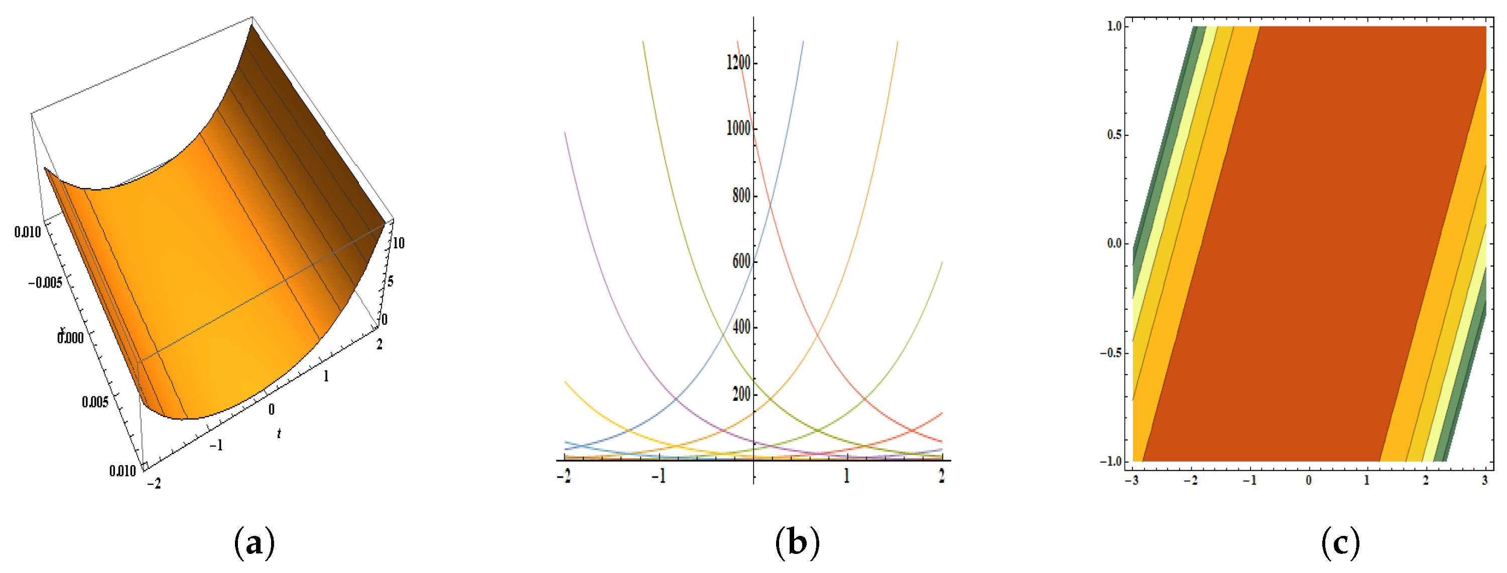
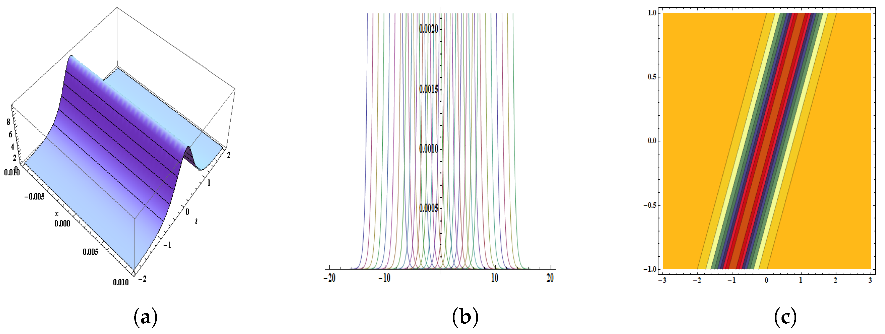
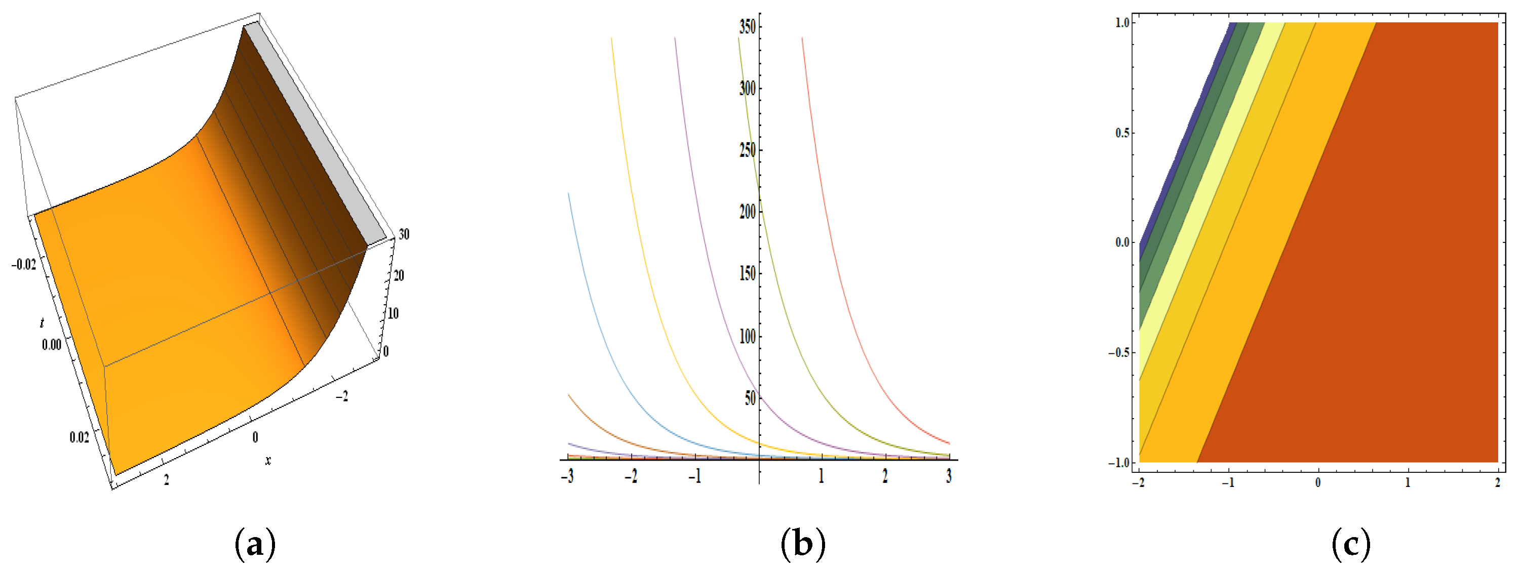
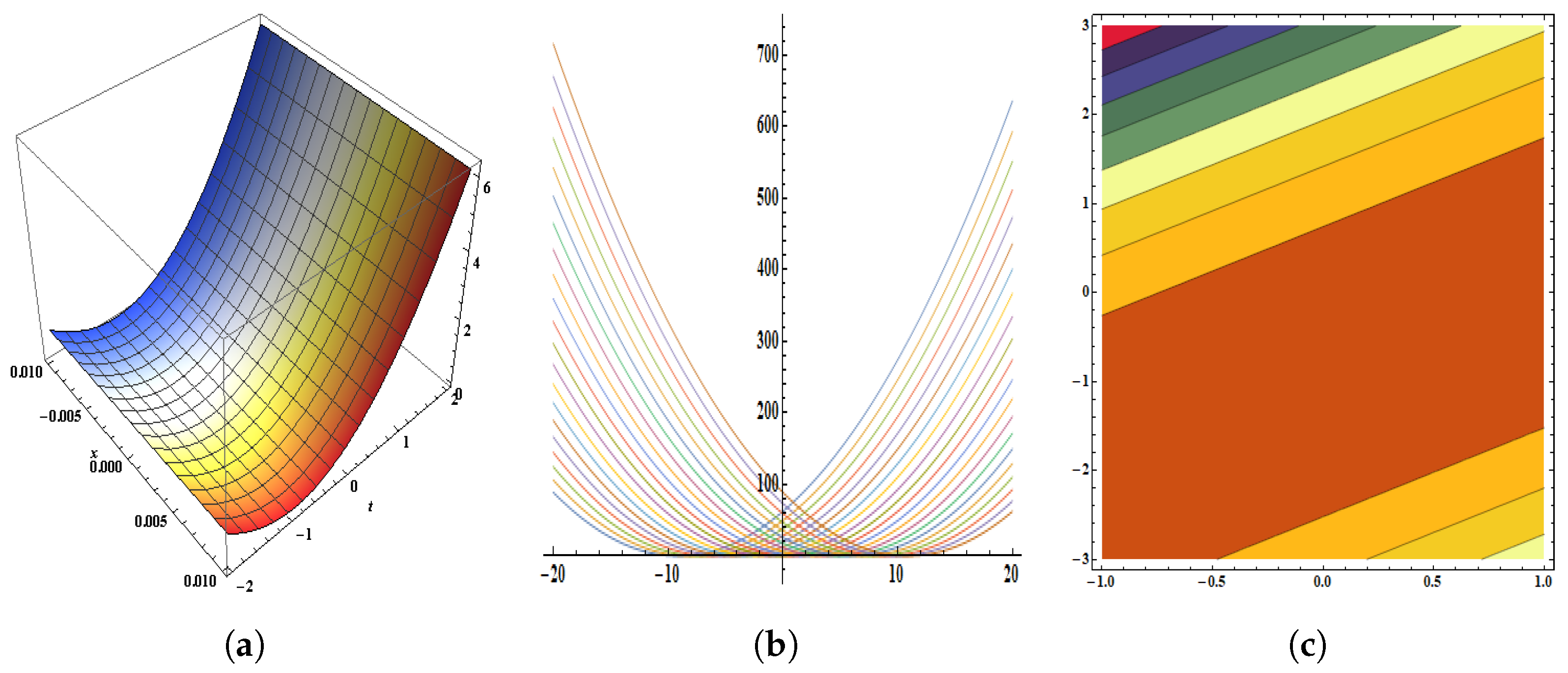
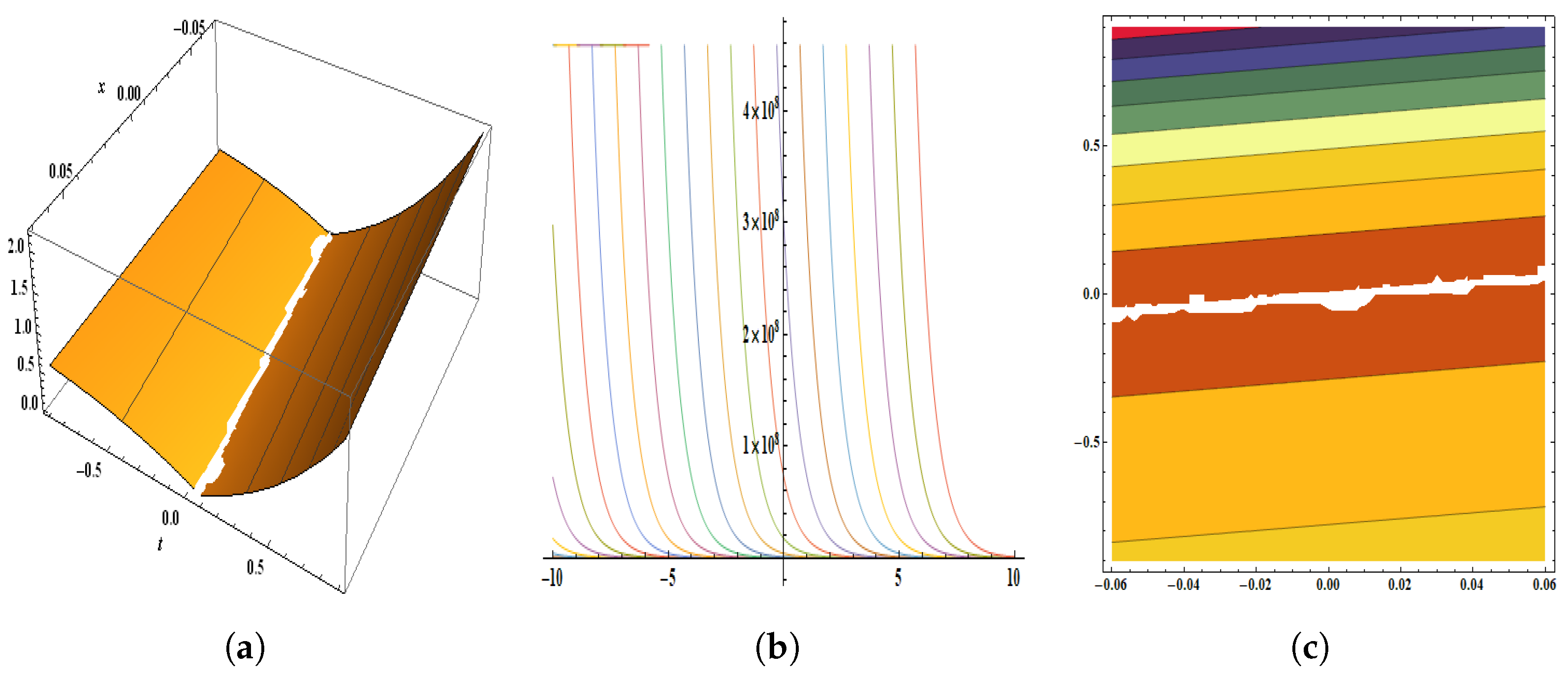
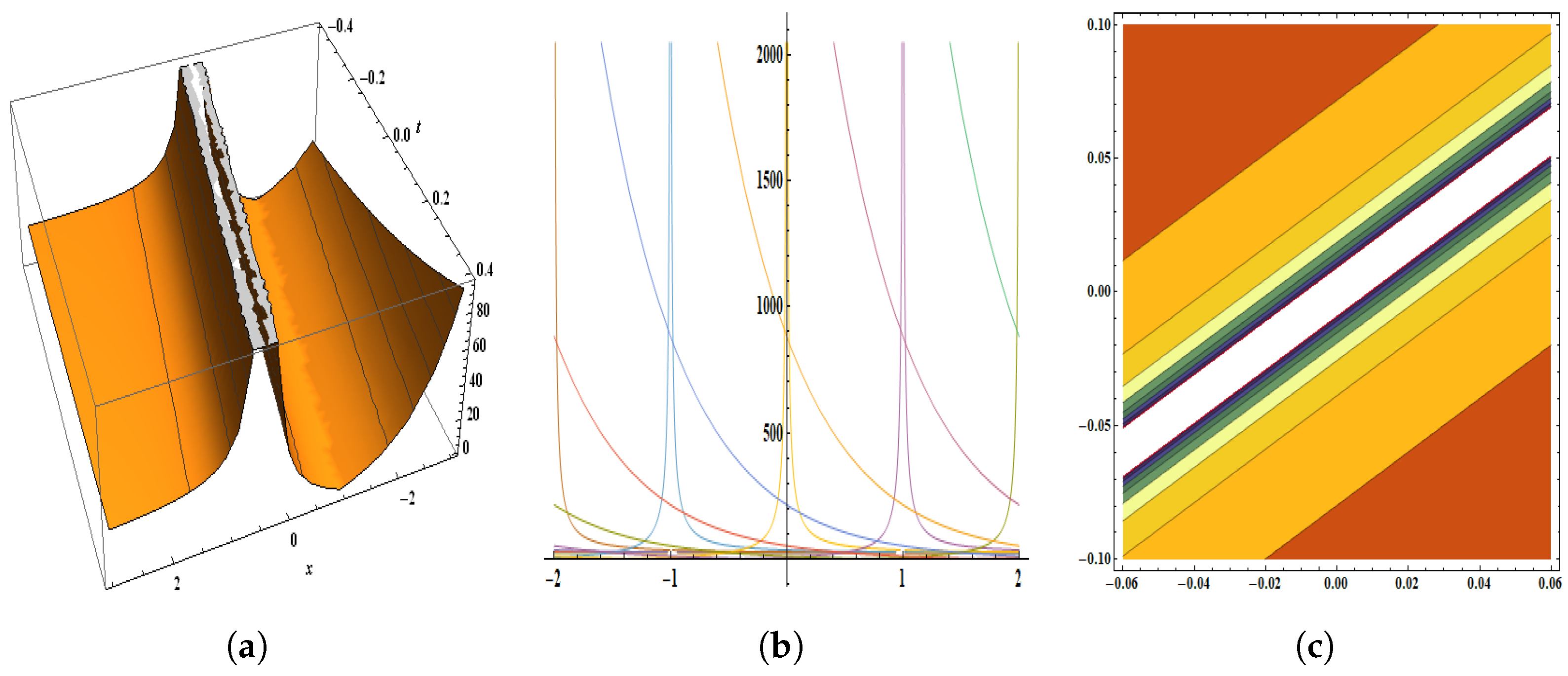
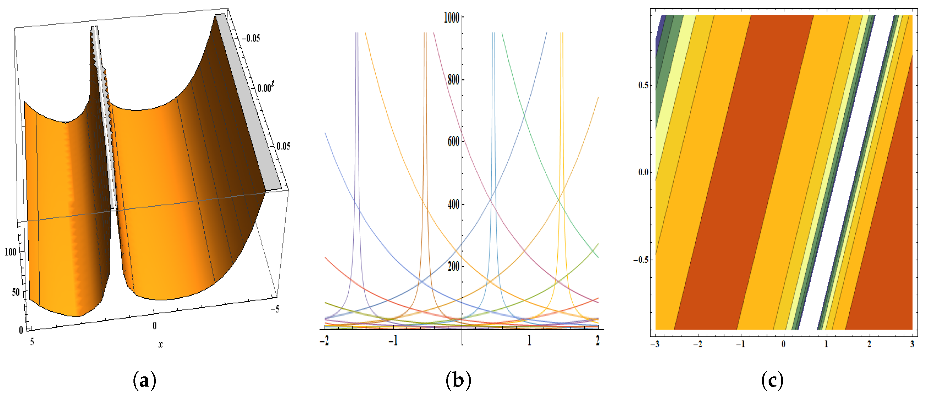
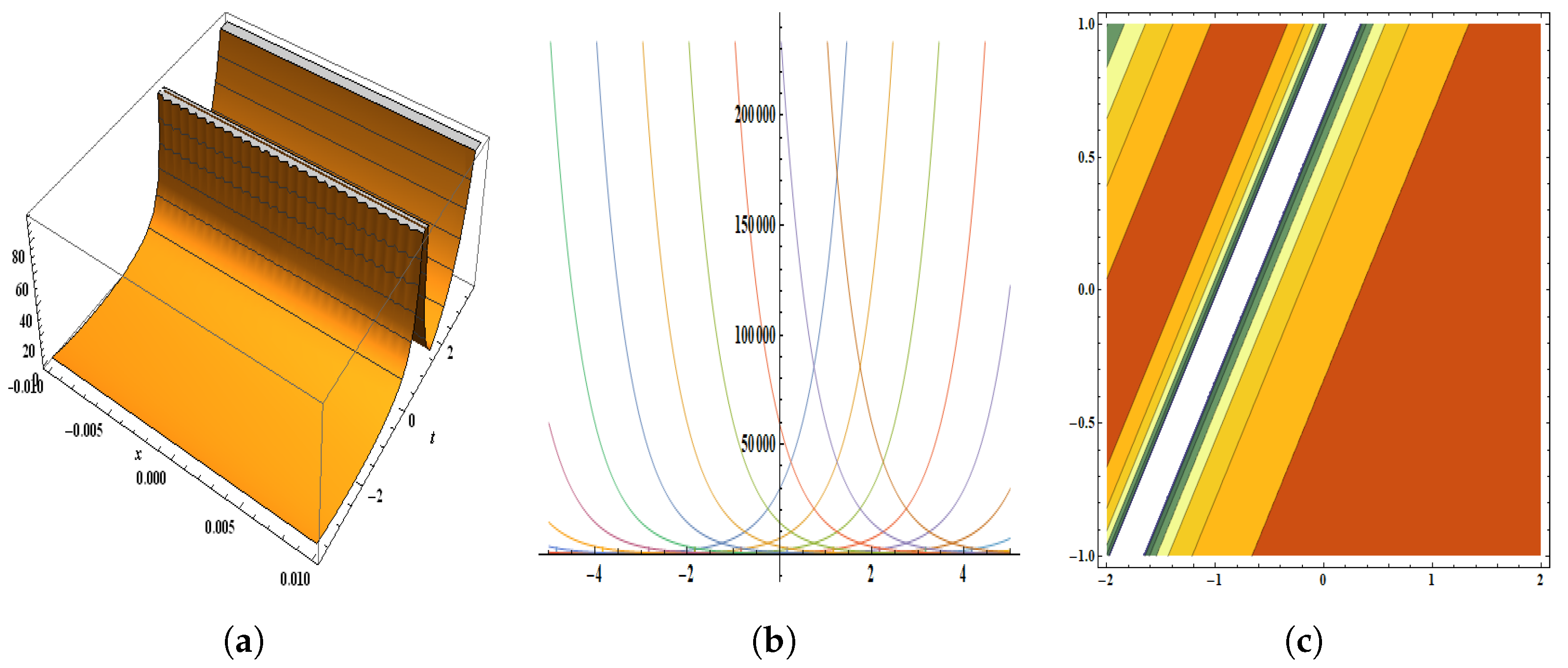
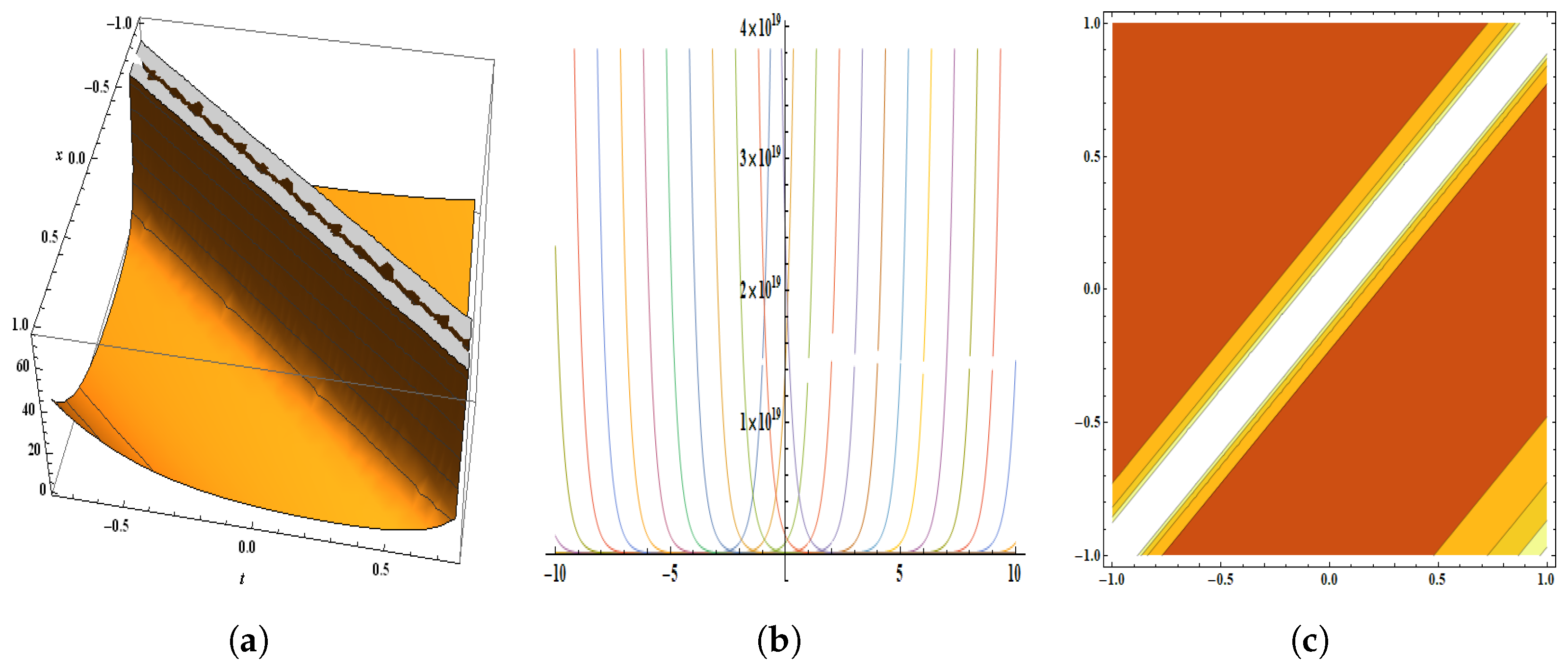
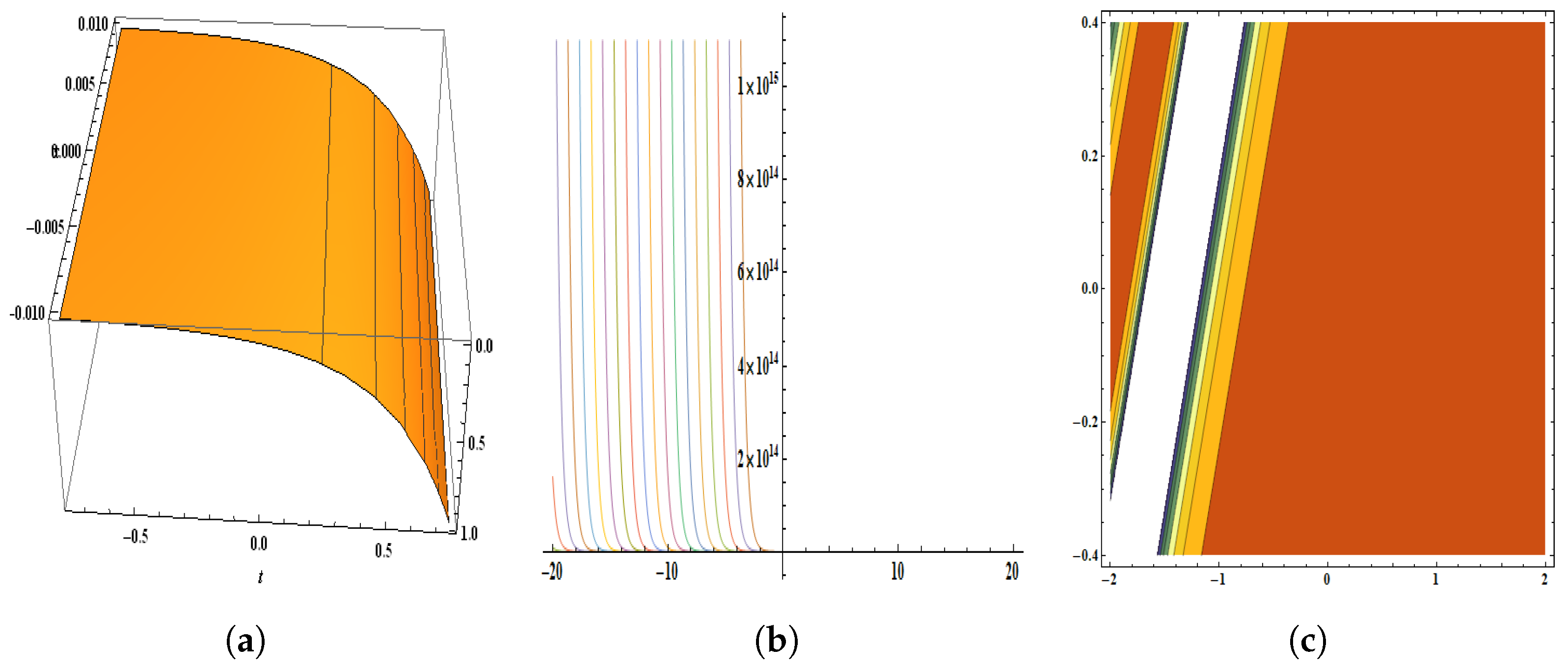
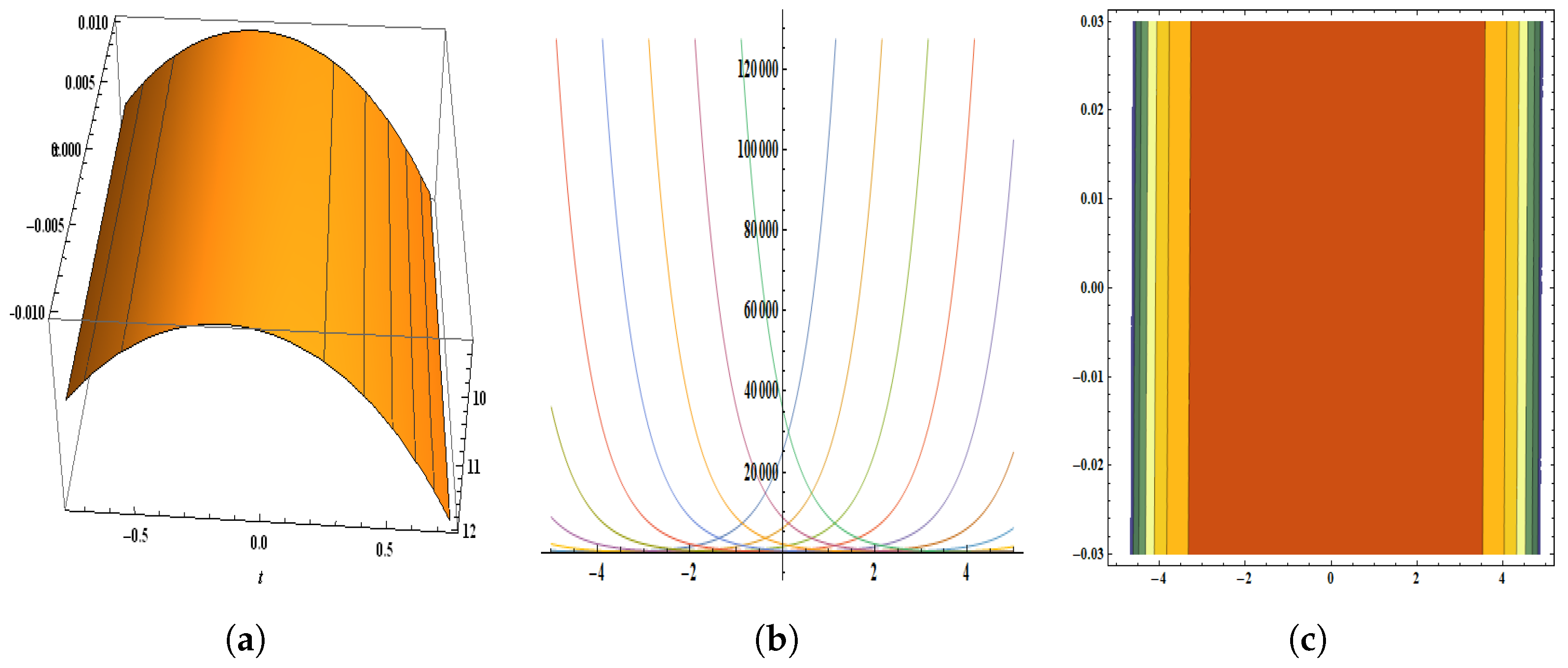
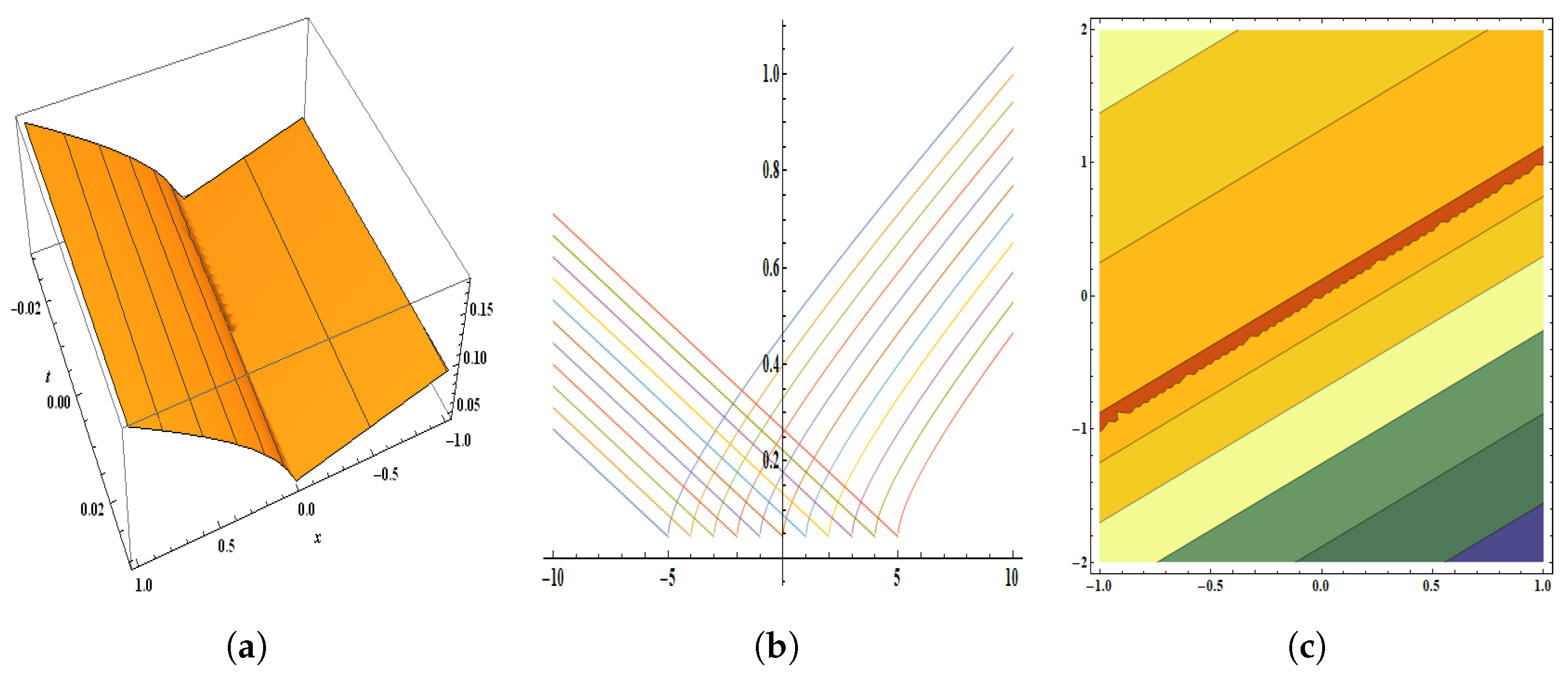
In this manuscript, the P-test was employed to check the integrability of TNFSEs. For the integrability, the first constant of the integration was calculated in Equation (15). The resonance was calculated in Equation (19). The other remaining constants of integrations were computed in Equations (22)–(25). There was no compatibility condition and both resonance conditions were verified. Therefore, the governing systems fully satisfied the P-test criteria. The AEM approach was implemented to obtain optical solitary wave solutions. Figure 1 show a smooth soliton solution Figure 2 show a bright soliton solution Figure 3 and Figure 4 also show a smooth soliton solution. Figure 5, Figure 6, Figure 7, Figure 8 and Figure 9 shows kink soliton solution. There is a singularity in its wave form. Figure 10, Figure 11 and Figure 12 shows smooth kink soliton solution. And Figure 13 shows bell kink soliton solution. Some of the solutions disclosed in this research study have not yet been published in the literature. These two approaches are simpler and more productive than other methods, they can also yield multiple soliton solutions at the same time, and they can also be applied to other FPDEs. More sophisticated and time-consuming algebraic computations can be performed with the help of mathematical packages (Mathematica). It is anticipated that the solutions presented here will be useful in further numerical analysis and will help in explaining some physical phenomena. This study is only an initial work, further applications to some other nonlinear physical systems can be explored and require considerable attention in many areas of physics and engineering, such as optics, fluid dynamics, plasma physics, and biological systems, where these obtained solitary wave solutions can be used. Optical communications, ocean wave modelling, plasma physics, and biological signal transmission are also some additional examples of their applications.
7. Conclusions
Using the mathematical computing software tool Mathematica, the P-test and the AEM technique were used to determine the integrability and some new optical solitary wave solutions of the TNFSE with modified RLD derivatives. These obtained solitons solutions are widely used in optics and photonics including the production of ultrafast laser pulses and the development of optical instruments for particle manipulation, while these soliton solutions are not directly used in most everyday applications, they do have significant indirect uses in domains such as communication, materials processing, and oceanography. There have been numerous graphical presentations of solitary periodic, kink-shaped, and singular solutions. These algorithms are efficient for finding a single exact solution and working with the nonlinear fractional governing equations existing in physics.
Author Contributions
Software, U.A.; Formal analysis, N.M.K.; Writing—original draft, I.A.K. All authors have read and agreed to the published version of the manuscript.
Funding
This research received no external funding.
Institutional Review Board Statement
We hereby declare that this manuscript is original, except for the quoted contents. This manuscript does not contain any research that has been published by others.
Data Availability Statement
Not applicable.
Conflicts of Interest
The authors declare no conflict of interest.
References
- Kumar, A.; Chauhan, H.V.S.; Ravichandran, C.; Nisar, K.S.; Baleanu, D. Existence of solutions of non-autonomous fractional differential equations with integral impulse condition. Adv. Differ. Equ. 2020, 2020, 434. [Google Scholar] [CrossRef]
- Shaikh, A.S.; Nisar, K.S. Transmission dynamics of fractional order Typhoid fever model using Caputo–Fabrizio operator. Chaos Solitons Fractals 2019, 128, 355–365. [Google Scholar] [CrossRef]
- Valliammal, N.; Ravichandran, C. Results on fractional neutral integro-differential systems with state-dependent delay in Banach spaces. Nonlinear Stud. 2018, 25, 159–171. [Google Scholar]
- Al-Smadi, M.; Arqub, O.A. Computational algorithm for solving fredholm time-fractional partial integrodifferential equations of dirichlet functions type with error estimates. Appl. Math. Comput. 2019, 342, 280–294. [Google Scholar] [CrossRef]
- Al-Smadi, M.; Freihat, A.; Khalil, H.; Momani, S.; Ali Khan, R. Numerical multistep approach for solving fractional partial differential equations. Int. J. Comput. Methods 2017, 14, 1750029. [Google Scholar] [CrossRef]
- Luchko, Y.; Gorenflo, R. Scale-invariant solutions of a partial differential equation of fractional order. Fract. Calc. Appl. Anal. 1998, 1, 63–78. [Google Scholar]
- Buckwar, E.; Luchko, Y. Invariance of a partial differential equation of fractional order under the Lie group of scaling transformations. J. Math. Anal. Appl. 1998, 227, 81–97. [Google Scholar] [CrossRef] [Green Version]
- Xu, Y.; He, Z. The short memory principle for solving Abel differential equation of fractional order. Comput. Math. Appl. 2011, 62, 4796–4805. [Google Scholar] [CrossRef] [Green Version]
- Veeresha, P.; Prakasha, D.G.; Kumar, S. A fractional model for propagation of classical optical solitons by using nonsingular derivative. Math. Methods Appl. Sci. 2020. [Google Scholar] [CrossRef]
- Hasan, S.; Al-Smadi, M.; El-Ajou, A.; Momani, S.; Hadid, S.; Al-Zhour, Z. Numerical approach in the Hilbert space to solve a fuzzy Atangana-Baleanu fractional hybrid system. Chaos Solitons Fractals 2021, 143, 110506. [Google Scholar] [CrossRef]
- Valliammal, N.; Ravichandran, C.; Nisar, K.S. Solutions to fractional neutral delay differential nonlocal systems. Chaos Solitons Fractals 2020, 138, 109912. [Google Scholar] [CrossRef]
- Kumar, S.; Ghosh, S.; Lotayif, M.S.; Samet, B. A model for describing the velocity of a particle in Brownian motion by Robotnov function based fractional operator. Alex. Eng. J. 2020, 59, 1435–1449. [Google Scholar] [CrossRef]
- Bekir, A.; Güner, O.; Cevikel, A.C. Fractional complex transform and exp-function methods for fractional differential equations. In Abstract and Applied Analysis; Hindawi: London, UK, 2013. [Google Scholar]
- Yakar, C.; Çiçek, M.; Gücen, M.B. Boundedness and Lagrange stability of fractional order perturbed system related to unperturbed systems with initial time difference in Caputo’s sense. Adv. Differ. Equ. 2011, 2011, 54. [Google Scholar] [CrossRef] [Green Version]
- Bashiri, T.; Vaezpour, S.M.; Nieto, J.J. Approximating solution of Fabrizio-Caputo Volterra’s model for population growth in a closed system by homotopy analysis method. J. Funct. Spaces 2018, 2018, 3152502. [Google Scholar] [CrossRef] [Green Version]
- Sene, N.; Abdelmalek, K. Analysis of the fractional diffusion equations described by Atangana-Baleanu-Caputo fractional derivative. Chaos Solitons Fractals 2019, 127, 158–164. [Google Scholar] [CrossRef]
- Scherer, R.; Kalla, S.L.; Tang, Y.; Huang, J. The Grünwald–Letnikov method for fractional differential equations. Comput. Math. Appl. 2011, 62, 902–917. [Google Scholar] [CrossRef] [Green Version]
- Aljahdaly, N.H.; Akgül, A.; Shah, R.; Mahariq, I.; Kafle, J. A Comparative Analysis of the Fractional-Order Coupled Korteweg–De Vries Equations with the Mittag–Leffler Law. J. Math. 2022, 2022, 8876149. [Google Scholar] [CrossRef]
- Javeed, S.; Baleanu, D.; Waheed, A.; Khan, M.S.; Affan, H. Analysis of homotopy perturbation method for solving fractional order differential equations. Mathematics 2019, 7, 40. [Google Scholar] [CrossRef] [Green Version]
- Odibat, Z.M.; Momani, S. Application of variational iteration method to nonlinear differential equations of fractional order. Int. J. Nonlinear Sci. Numer. Simul. 2006, 7, 27–34. [Google Scholar] [CrossRef]
- Agarwal, P.; Karimov, E.; Mamchuev, M.; Ruzhansky, M. On boundary-value problems for a partial differential equation with Caputo and Bessel operators. In Recent Applications of Harmonic Analysis to Function Spaces, Differential Equations, and Data Science; Springer: Berlin, Germany, 2017; pp. 707–718. [Google Scholar]
- Al-Smadi, M.; Arqub, O.A.; Momani, S. Numerical computations of coupled fractional resonant Schrödinger equations arising in quantum mechanics under conformable fractional derivative sense. Phys. Scr. 2020, 95, 075218. [Google Scholar] [CrossRef]
- Feynman, R.P.; Hibbs, A.R.; Styer, D.F. Quantum Mechanics and Path Integrals; Courier Corporation: North Chelmsford, MA, USA, 2010. [Google Scholar]
- Laskin, N. Fractional Schrödinger equation. Phys. Rev. E 2012, 66, 056108. [Google Scholar] [CrossRef] [Green Version]
- Laskin, N. Fractional quantum mechanics and Lévy path integrals. Phys. Lett. A 2000, 268, 298–305. [Google Scholar] [CrossRef] [Green Version]
- Naber, M. Time fractional Schrödinger equation. J. Math. Phys. 2004, 45, 3339–3352. [Google Scholar] [CrossRef] [Green Version]
- Muslih, S.I.; Agrawal, O.P.; Baleanu, D. A Fractional Schrödinger Equation and Its Solution. Int. J. Theor. Phys. 2010, 49, 1746–1752. [Google Scholar] [CrossRef]
- Messiah, A. Quantum Mechanics; Courier Corporation: North Chelmsford, MA, USA, 2014. [Google Scholar]
- Guo, B.; Han, Y.; Xin, J. Existence of the global smooth solution to the period boundary value problem of fractional nonlinear Schrödinger equation. Appl. Math. Comput. 2008, 204, 468–477. [Google Scholar] [CrossRef]
- Jumarie, G. An approach to differential geometry of fractional order via modified Riemann-Liouville derivative. Acta Math. Sin. Engl. Ser. 2019, 28, 1741–1768. [Google Scholar] [CrossRef]
- Jumarie, G. Table of some basic fractional calculus formulae derived from a modified Riemann–Liouville derivative for non-differentiable functions. Appl. Math. Lett. 2009, 22, 378–385. [Google Scholar] [CrossRef]
- Iomin, A. Fractional-time Schrödinger equation: Fractional dynamics on a comb. Chaos Solitons Fractals 2011, 44, 348–352. [Google Scholar] [CrossRef] [Green Version]
- Tofighi, A. Probability structure of time fractional Schrödinger equation. Acta Phys. Pol.-Ser. A Gen. Phys. 2009, 116, 114. [Google Scholar] [CrossRef]
- Alabedalhadi, M. Exact travelling wave solutions for nonlinear system of spatiotemporal fractional quantum mechanics equations. Alex. Eng. J. 2022, 61, 1033–1044. [Google Scholar] [CrossRef]
- Hulstman, M.V. The Painlevé analysis and exact travelling wave solutions to nonlinear partial differential equations. Math. Comput. Model. 1993, 18, 151–156. [Google Scholar] [CrossRef]
- Iqbal, M.; Zhang, Y. Painlevé analysis for (2 + 1)-dimensional non-linear Schrödinger equation. Appl. Math. 2017, 8, 1539–1545. [Google Scholar] [CrossRef] [Green Version]
- Ablowitz, M.J.; Ramani, A.; Segur, H.A. Connection between nonlinear evolution equations and ordinary differential equation of P-type. J. Math. Phys. 1980, 21, 715–721. [Google Scholar] [CrossRef]
- Weiss, J.; Tabor, M.; Carnevale, G. The Painlevé property for partial differential equations. J. Math. Phys. 1983, 24, 522–526. [Google Scholar] [CrossRef]
- Ramani, A.; Grammaticos, B.; Bountis, T. The Painlevé property and singularity analysis of integrable and non-integrable systems. Phys. Rep. 1989, 180, 159–245. [Google Scholar] [CrossRef]
- Baldwin, D.E. Symbolic Algorithms and Software for the Painlevé Test and Recursion Operator for Nonlinear Partial Diffrential Equations. Ph.D. Thesis, Colorado School of Mines, Golden, CO, USA, 2004. [Google Scholar]
- Abdou, M.A. A generlaized auxiliary equation method and its applications. Nonlinear Dyn. 2008, 52, 95–102. [Google Scholar] [CrossRef]
- Seadawy, A.R.; Cheemaa, N. Application of extended modified auxiliary equation mapping method for high order dispersive extended nonlinear Schrödinger equation in nonlinear optics. Mod. Phys. Lett. B 2019, 33, 1950203. [Google Scholar] [CrossRef]
- Wu, G.Z.; Yu, L.J.; Wang, Y.Y. Fractional optical solitons of the space-time fractional nonlinear Schrödinger equation. Optik 2020, 207, 164405. [Google Scholar] [CrossRef]
- Rezazadeh, H.; Odabasi, M.; Tariq, K.U.; Abazari, R.; Baskonus, H.M. On the conformable nonlinear Schrödinger equation with second order spatiotemporal and group velocity dispersion coefficients. Chin. J. Phys. 2021, 72, 403–414. [Google Scholar] [CrossRef]
- Liang, X.; Khaliq, A.Q.M.; Bhatt, H.; Furati, K.M. The locally extrapolated exponential splitting scheme for multi-dimensional nonlinear space-fractional Schrödinger equations. Numer. Algorithms 2017, 76, 939–958. [Google Scholar] [CrossRef]
- Abdel-Salam, E.A.B.; Yousif, E.A. Solution of nonlinear space-time fractional differential equations using the fractional Riccati expansion method. Math. Probl. Eng. 2013, 2013, 846283. [Google Scholar] [CrossRef]
- Li, M.; Gu, X.M.; Huang, C.; Fei, M.; Zhang, G. A fast linearized conservative finite element method for the strongly coupled nonlinear fractional Schrödinger equations. J. Comput. Phys. 2018, 358, 256–282. [Google Scholar] [CrossRef]
- Guo, B.; Huang, D. Existence and stability of standing waves for nonlinear fractional Schrödinger equations. J. Math. Phys. 2012, 53, 083702. [Google Scholar] [CrossRef]
Figure 1.
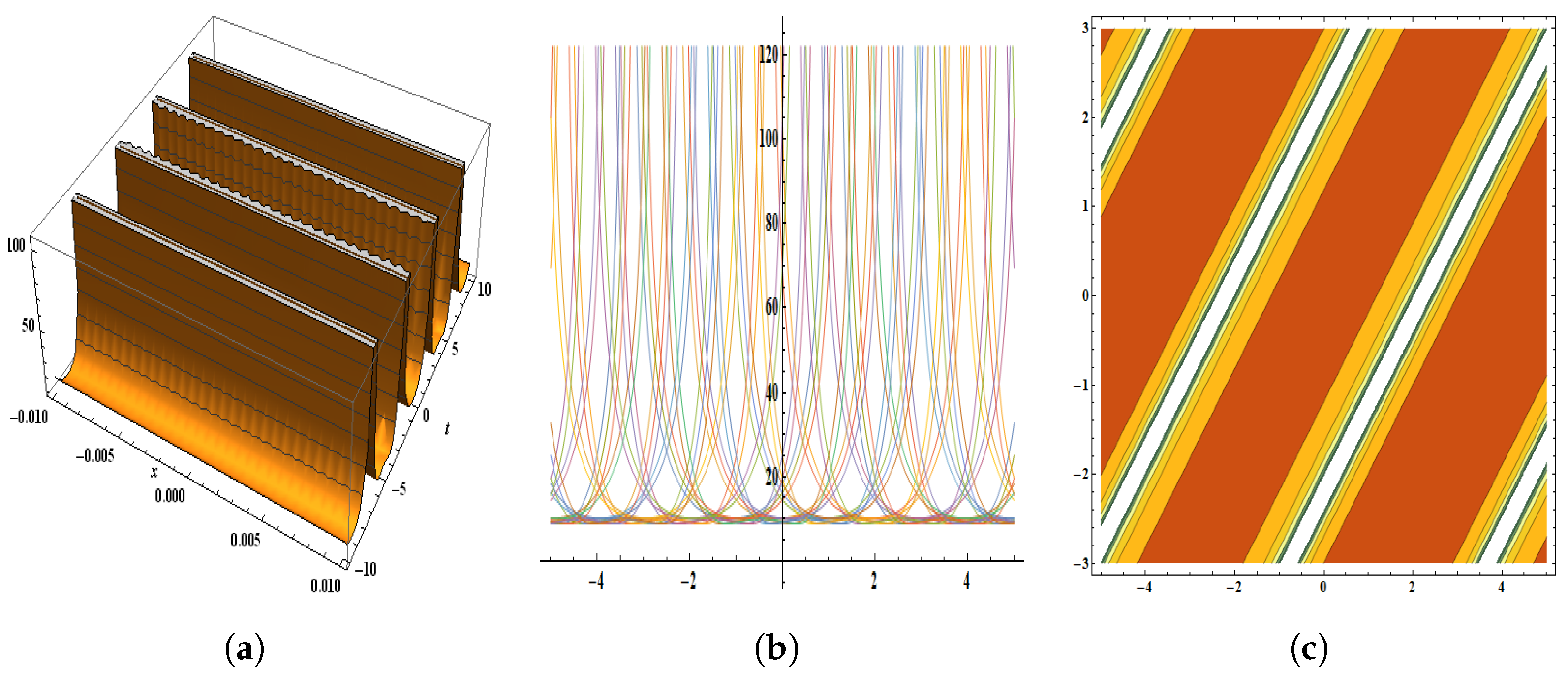
The parameters are , , , , , , , , , and . The figure provides a pictorial illustration of : (a) displays the 3D plot in [−0.01, 0.01] and [−2, 2], (b) displays the 2D plot in [−2, 2] and [−5, 5], (c) displays the contour plot.
Figure 1.
The parameters are , , , , , , , , , and . The figure provides a pictorial illustration of : (a) displays the 3D plot in [−0.01, 0.01] and [−2, 2], (b) displays the 2D plot in [−2, 2] and [−5, 5], (c) displays the contour plot.

Figure 2.
The parameters are , , , , , , , , , , , and . The figure provides the pictorial illustration of : (a) displays the 3D plot in [−0.01, 0.01] and [−2, 2], (b) displays the 2D plot in [−20, 20] and [−10, 10], (c) displays the contour plot.
Figure 2.
The parameters are , , , , , , , , , , , and . The figure provides the pictorial illustration of : (a) displays the 3D plot in [−0.01, 0.01] and [−2, 2], (b) displays the 2D plot in [−20, 20] and [−10, 10], (c) displays the contour plot.

Figure 3.
The parameters are , , , , , , , , , , and . The figure provides the pictorial illustration of : (a) displays the 3D plot in [−3, 3] and [−0.03, 0.03], (b) displays the 2D plot in [−3, 3] and [−5, 5], (c) displays the contour plot.
Figure 3.
The parameters are , , , , , , , , , , and . The figure provides the pictorial illustration of : (a) displays the 3D plot in [−3, 3] and [−0.03, 0.03], (b) displays the 2D plot in [−3, 3] and [−5, 5], (c) displays the contour plot.

Figure 4.
The parameters are , , , , , , , , , , and . The figure provides the pictorial illustration of : (a) displays the 3D plot in [−1, 1] and [−0.01, 0.01], (b) displays the 2D plot in [−10, 10] and [−20, 20], (c) displays the contour plot.
Figure 4.
The parameters are , , , , , , , , , , and . The figure provides the pictorial illustration of : (a) displays the 3D plot in [−1, 1] and [−0.01, 0.01], (b) displays the 2D plot in [−10, 10] and [−20, 20], (c) displays the contour plot.

Figure 5.
The parameters are , , , , , , , , , , and . The figure provides the pictorial illustration of : (a) displays the 3D plot in [−0.07, 0.07] and [−0.9, 0.9], (b) displays the 2D plot in [−10, 10] and [−20, 20], (c) displays the contour plot.
Figure 5.
The parameters are , , , , , , , , , , and . The figure provides the pictorial illustration of : (a) displays the 3D plot in [−0.07, 0.07] and [−0.9, 0.9], (b) displays the 2D plot in [−10, 10] and [−20, 20], (c) displays the contour plot.

Figure 6.
The parameters are , , , , , , , , , , and . The figure provides the pictorial illustration of : (a) displays the 3D plot in [−3, 3] and [−0.4, 0.4], (b) displays the 2D plot in [−7, 7] and [−2, 2], (c) displays the contour plot.
Figure 6.
The parameters are , , , , , , , , , , and . The figure provides the pictorial illustration of : (a) displays the 3D plot in [−3, 3] and [−0.4, 0.4], (b) displays the 2D plot in [−7, 7] and [−2, 2], (c) displays the contour plot.

Figure 7.
The parameters are , , , , , , , , , , and . The figure provides the pictorial illustration of : (a) displays the 3D plot in [−3, 3] and [−0.4, 0.4], (b) displays the 2D plot in [−7, 7] and [−2, 2], (c) displays the contour plot.
Figure 7.
The parameters are , , , , , , , , , , and . The figure provides the pictorial illustration of : (a) displays the 3D plot in [−3, 3] and [−0.4, 0.4], (b) displays the 2D plot in [−7, 7] and [−2, 2], (c) displays the contour plot.

Figure 8.
The parameters are , , , , , , , , , and . Pictorial illustration of : (a) displays the 3D plot in [−0.01, 0.01] and [−3.75, 3.75], (b) displays the 2D plot in [−5, 5] and [−10, 10], (c) displays the contour plot.
Figure 8.
The parameters are , , , , , , , , , and . Pictorial illustration of : (a) displays the 3D plot in [−0.01, 0.01] and [−3.75, 3.75], (b) displays the 2D plot in [−5, 5] and [−10, 10], (c) displays the contour plot.

Figure 9.
The parameters are , , , , , , , , , and . Pictorial illustration of : (a) displays the 3D plot in [−1, 1] and [−0.75, 0.75], (b) displays the 2D plot in [−10, 10] and [−17, 17], (c) displays the contour plot.
Figure 9.
The parameters are , , , , , , , , , and . Pictorial illustration of : (a) displays the 3D plot in [−1, 1] and [−0.75, 0.75], (b) displays the 2D plot in [−10, 10] and [−17, 17], (c) displays the contour plot.

Figure 10.
The parameters are , , , , , , , , , , and . The figure provides the pictorial illustration of : (a) displays the 3D plot in [−0.01, 0.01] and [−0.75, 0.75], (b) displays the 2D plot in [−20, 20] and [−10, 10], (c) displays the contour plot.
Figure 10.
The parameters are , , , , , , , , , , and . The figure provides the pictorial illustration of : (a) displays the 3D plot in [−0.01, 0.01] and [−0.75, 0.75], (b) displays the 2D plot in [−20, 20] and [−10, 10], (c) displays the contour plot.

Figure 11.
The parameters are , , , , , , , , , , and . The figure provides the pictorial illustration of : (a) displays the 3D plot in [−0.01, 0.01] and [−0.75, 0.75], (b) displays the 2D plot in [−5, 5] and [−7, 7], (c) displays the contour plot.
Figure 11.
The parameters are , , , , , , , , , , and . The figure provides the pictorial illustration of : (a) displays the 3D plot in [−0.01, 0.01] and [−0.75, 0.75], (b) displays the 2D plot in [−5, 5] and [−7, 7], (c) displays the contour plot.

Figure 12.
The parameters are , , , , , , , , , , and . The figure provides the pictorial illustration of : (a) displays the 3D plot in [−1, 1] and [−0.03, 0.03], (b) displays the 2D plot in [−5, 5] and [−10, 10], (c) displays the contour plot.
Figure 12.
The parameters are , , , , , , , , , , and . The figure provides the pictorial illustration of : (a) displays the 3D plot in [−1, 1] and [−0.03, 0.03], (b) displays the 2D plot in [−5, 5] and [−10, 10], (c) displays the contour plot.

Figure 13.
The parameters are , , , , , , , , , and . The figure provides the pictorial illustration of : (a) displays the 3D plot in [−0.01, 0.01] and [−10, 10], (b) displays the 2D plot in [−5, 5] and [−10, 10], (c) displays the contour plot.
Figure 13.
The parameters are , , , , , , , , , and . The figure provides the pictorial illustration of : (a) displays the 3D plot in [−0.01, 0.01] and [−10, 10], (b) displays the 2D plot in [−5, 5] and [−10, 10], (c) displays the contour plot.

Disclaimer/Publisher’s Note: The statements, opinions and data contained in all publications are solely those of the individual author(s) and contributor(s) and not of MDPI and/or the editor(s). MDPI and/or the editor(s) disclaim responsibility for any injury to people or property resulting from any ideas, methods, instructions or products referred to in the content. |
© 2023 by the authors. Licensee MDPI, Basel, Switzerland. This article is an open access article distributed under the terms and conditions of the Creative Commons Attribution (CC BY) license (https://creativecommons.org/licenses/by/4.0/).
Share and Cite
MDPI and ACS Style
Khoso, I.A.; Katbar, N.M.; Akram, U. Optical Dromions for Spatiotemporal Fractional Nonlinear System in Quantum Mechanics. Quantum Rep. 2023, 5, 546-564. https://0-doi-org.brum.beds.ac.uk/10.3390/quantum5030036
AMA Style
Khoso IA, Katbar NM, Akram U. Optical Dromions for Spatiotemporal Fractional Nonlinear System in Quantum Mechanics. Quantum Reports. 2023; 5(3):546-564. https://0-doi-org.brum.beds.ac.uk/10.3390/quantum5030036
Chicago/Turabian StyleKhoso, Ihsan A., Nek Muhammad Katbar, and Urooj Akram. 2023. "Optical Dromions for Spatiotemporal Fractional Nonlinear System in Quantum Mechanics" Quantum Reports 5, no. 3: 546-564. https://0-doi-org.brum.beds.ac.uk/10.3390/quantum5030036