
The Quantum Amplitude Estimation Algorithms on Near-Term Devices: A Practical Guide


1
Istituto di Fotonica e Nanotecnologie, Consiglio Nazionale delle Ricerche, Piazza Leonardo da Vinci 32, 20133 Milano, Italy
2
Department of Pharmacy and Biotechnology, University of Bologna, Via Belmeloro 6, 40126 Bologna, Italy
3
Data Reply s.r.l., Corso Francia, 110, 10143 Torino, Italy
4
Dipartimento di Informatica, Universita di Verona, Strada Le Grazie, 15, 37134 Verona, Italy
5
Dipartimento di Fisica, Universita di Milano, Via Celoria 16, 20133 Milano, Italy
6
National Inter-University Consortium for Telecommunications (CNIT), Viale G.P. Usberti, 181/A Pal.3, 43124 Parma, Italy
*
Author to whom correspondence should be addressed.
Quantum Rep. 2024, 6(1), 1-13; https://0-doi-org.brum.beds.ac.uk/10.3390/quantum6010001
Submission received: 9 October 2023
/
Revised: 17 November 2023
/
Accepted: 25 November 2023
/
Published: 24 December 2023
(This article belongs to the Special Issue Quantum Computing: A Taxonomy, Systematic Review, and Future Directions)
Abstract
:The Quantum Amplitude Estimation (QAE) algorithm is a major quantum algorithm designed to achieve a quadratic speed-up. Until fault-tolerant quantum computing is achieved, being competitive over classical Monte Carlo (MC) remains elusive. Alternative methods have been developed so as to require fewer resources while maintaining an advantageous theoretical scaling. We compared the standard QAE algorithm with two Noisy Intermediate-Scale Quantum (NISQ)-friendly versions of QAE on a numerical integration task, with the Monte Carlo technique of Metropolis–Hastings as a classical benchmark. The algorithms were evaluated in terms of the estimation error as a function of the number of samples, computational time, and length of the quantum circuits required by the solutions, respectively. The effectiveness of the two QAE alternatives was tested on an 11-qubit trapped-ion quantum computer in order to verify which solution can first provide a speed-up in the integral estimation problems. We concluded that an alternative approach is preferable with respect to employing the phase estimation routine. Indeed, the Maximum Likelihood estimation guaranteed the best trade-off between the length of the quantum circuits and the precision in the integral estimation, as well as greater resistance to noise.
1. Introduction
We surveyed and implemented different versions of the Quantum Amplitude Estimation (QAE) algorithm, and we found that the Maximum Likelihood QAE, which does not make use of phase estimation, resulted in being the best candidate to demonstrate an advantage over the classical Monte Carlo methods. Numerical integration is a fundamental problem in many areas of science and engineering. Traditional numerical integration methods can be computationally expensive and require significant computational resources. Monte Carlo (MC) methods [1] are exploited for numerical integration problems, as they are flexible and able to handle high-dimensional problems. However, Monte Carlo methods are limited in terms of approximation accuracy, which depends on the number of samples used in the simulation. Indeed, such a class of methods suffers from the difficulty of generating good sampling by starting from an arbitrary probability density function. As a result, Monte Carlo methods can be computationally expensive for high-precision integration, making them less efficient for certain applications [2]. Quantum computing [3,4,5,6,7,8,9] provides an alternative path to obtain faster integral estimation, with the same accuracy with fewer samples. Such a speed-up was made possible by the introduction of the Quantum Amplitude Estimation algorithm [10]. QAE is a quantum algorithm that can be used to estimate the amplitude of a specific state in a quantum system with quantum speed-up compared to classical algorithms. Such a feature allows QAE to be used for the efficient numerical integration of complex functions. In particular, QAE has been shown to be able to beat the classical Monte Carlo methods for numerical integration, especially in high-dimensional integration problems. By using QAE, it is possible to estimate the integrals with the same precision by extracting fewer samples, thus significantly reducing the computational resources required for numerical integration. Moreover, QAE can be used to solve a wide range of numerical integration problems, including those in finance [11], physics [12,13], and machine learning [14,15,16,17]. It has been shown that QAE can be applied to estimate options pricing [18] in financial derivatives [19,20], to solve differential equations [21], and to perform quantum simulation, among others. The QAE algorithm carries a quadratic speed-up with respect to classic Monte Carlo techniques. However, such an advantage is constrained by the existence of fault-tolerant quantum hardware [22,23,24,25,26,27,28], which does not exist today. In currently available Noisy Intermediate-Scale Quantum (NISQ) devices [29], the QAE algorithm has not yet shown an advantage in practical cases [30] due to the insufficient coherence times of the physical qubits [31] and because of the error carried by the gates. Indeed, the QAE circuit involves applications of controlled quantum queries and a quantum Fourier transform. Therefore, alternative approaches have been proposed for QAE that involve a lower-depth circuit. Such quantum–classical hybrid algorithms can be divided into two categories, namely the Maximum Likelihood Quantum Amplitude Estimation (MLQAE) [32] approach and the Iterative QAE (IQAE) [33] approach, respectively.
A major difference consists of the fact that, while the MLAE approach allows fixing the number of quantum queries, in the iterative approach, such a number is classically computed at each iteration from the result of the previous one. Therefore, the way errors propagate during the runs is not trivial. For this reason, it is necessary to evaluate the performance of such methods on noisy devices to determine which one best realizes its purpose. The performance analysis of such methods has been, then, divided into two steps. First, the analysis is carried out with the use of a quantum computing simulator. Here, the standard QAE, the MLAE, the IQAE, and the classical Metropolis–Hastings Monte Carlo (MHMC) algorithms were compared. The scaling on the estimation error, the execution time, and the depth of the circuits were considered, respectively. A 1D integral was used to exemplify and benchmark, providing a reasonable trade-off between being representative and carrying an addressable circuit depth. All simulations were performed on the quantum circuit simulator ‘aer_simulator’ of the Qiskit library, by involving three qubits. The second part of the analysis instead involved the use of quantum hardware with the specific aim of determining the degree of resilience of the methods with respect to the noise of the hardware. For such an analysis, the trapped-ion device Harmony from IonQ was used. The trapped-ion qubits are well-known for their superior coherence and fidelity [34]. Such processors have already shown that they can support quantum circuits with a depth greater than other technologies [35]. For this reason, it represents an adequate candidate for benchmarking amplitude estimation solutions. The MLQAE method appears to be a more-short-term alternative to the standard QAE for estimating integrals. The iterative method, on the other hand, is more sensitive to the noise of the quantum processing unit (QPU). Moreover, the iterative hybrid approach has a greater depth of the circuits that implement it on average. Furthermore, it requires deeper circuits than the MLAE approach in terms of scaling with respect to the estimation error. Instead, the two approaches exhibit a comparable speed-up. The article is divided into Sections as follows: The standard QAE and its application to the numerical integration problem are defined in Section 2.1. Section 2.2 presents the NISQ-friendly alternatives of QAE. The results are divided into a presentation of the noiseless simulations in Section 3 and the execution on the real trapped-ion device used for the benchmarking—described in Section 4.1—in Section 4.2.
2. Quantum Amplitude Estimation Algorithms
Quantum Amplitude Estimation (QAE) [10] is a fundamental quantum algorithm with the potential to achieve a quadratic speed-up for many applications that are classically solved through Monte Carlo (MC) simulation [13]. QAE is of particular interest for its exploitation in finance, including, for instance, risk analysis and options pricing, as well as more-general tasks such as numerical integration. This Section is divided as follows: In Section 2.1, the original QAE algorithm is summarized. Section 2.2 reports on state-of-the-art alternative methods to the original version. The process is pictured in Figure 1.
2.1. Original Quantum Amplitude Estimation Algorithm
In this Section, the original version of the QAE, for numerical integration, is summarized. In order to introduce it, let us first consider an integral:
over the integration domain X, and let us define a probability distribution such that for , then the integral can be rewritten as
where in X and 0 otherwise. Classically, the Monte Carlo method consists of a set of methods to estimate the integral in Equation (2). Such methods start from the assumption of sampling M values from and, then, estimating I with the average estimator.
The estimation error bound of classical MC simulation scales as , where M denotes the number of (classical) samples. Instead, the quantum algorithm called QAE allows achieving a quadratic speed-up as explained below. The QAE problem can be stated as follows: given an operator acting on qubits,
where is the probability to measure the ancilla qubit in 1 and it is unknown [10]; and are two normalized states, not necessarily orthogonal [33].
Let us define an operator , where , representing reflection with respect to the state , while the reflection with respect to the state . Applications of are denoted as quantum samples or oracle queries [33].
The canonical QAE follows the form of quantum phase estimation (QPE): (i) it uses m ancilla qubits, initialized in equal superposition, to represent the final result; (ii) it defines the number of quantum samples as ; (iii) it applies geometrically increasing powers of controlled by the ancilla qubits. Eventually, it performs an inverse quantum Fourier transform (QFT) on the ancilla qubits before they are measured. The measurement of m ancilla qubits produces a bit string equivalent to an integer , and an estimation of a can be defined as , where . The algorithm produces an estimation such that
with a probability
where , while is the minimal distance on the unit circle between the angles and , therefore returning a scaling complexity of for M applications of quantum samples .
The success probability to obtain with the discrepancy shown in Equation (5) can be quickly boosted to close to by repeating the QAE circuit multiple times and by using the median estimate. Since the success probability of QAE is greater than we would, in principle, only need, for instance, 24 repetitions to achieve a success probability of [30]. However, current quantum hardware introduces additional errors. In the work [30], the circuit was repeated 8192 times to obtain a reliable estimate of a.
2.2. Alternative Quantum Amplitude Estimation Methods
As discussed, current hardware limitations prevent the achievement of the theoretical speed-up. For this reason, various algorithms have been developed involving both classical and quantum devices in order to reduce the resources required for quantum computation without denying a speed-up against Monte Carlo methods. The alternative hybrid algorithms can be divided into two categories. The first category (I), which we will refer to as a Maximum Likelihood Amplitude Estimation (MLAE) approach, consists of a Grover-like circuit and a Maximum Likelihood estimation on a classical processor. Such an approach has been discussed by different groups: in Ref. [32], the idea was introduced for the first time, while two variants were proposed later [36,37].
The second category (II), under the name of iterative approaches, consists of an alternating sequence of Grover-like circuits, where the oracle query is applied k times, and a classical algorithm to compute the value k of applications for the next quantum iteration. Such an iterative procedure leads to a decrease in the confidence interval of the estimation up to the error with up to iterations [33]. Such an algorithm, in turn, is inspired by the variant of the quantum approximation counting described by Aaronson and Rall [38].
2.2.1. MLAE Approach
As mentioned earlier, such a quantum–classical hybrid class of algorithms involves both a Grover-like circuit and a Maximum Likelihood Estimation (MLE) [39] on a classical processor, respectively. In the following, the strategy of the algorithm is analyzed. Let be an operator such that
The aim of the algorithm is to estimate . It is possible to replace the QPE with a set of Grover iterations combined with a Maximum Likelihood Estimation (MLE) [32].
Let us perform sampling from the circuit:
From Equation (8), we are able to model the probability distribution of the measurements of the ancilla qubit with and .
The likelihood of such a model is
where is the number of measurements that have returned 1 and is the total number of measurements.
Next, let us perform the sampling times with in order to compute the total likelihood:
Using the Maximum Likelihood procedure, we are able to compute the optimal such that our model approximates the true distribution as closely as possible:
Now, a and are uniquely related through in the range so , as the function is invertible in such an interval. As shown in Ref. [36], a pure MLAE method, as described above, provides less than a quadratic advantage compared to classical Monte Carlo. The paper introduces an algorithm that utilizes the MLAE method, but alternates it with a variational optimization step.
2.2.2. Iterative Approach
As in the previously discussed approach, the IQAE replaces the standard QAE circuit with the low-complexity circuit defined in Equation (8). The difference between the two approaches is that, while in the MLAE method, the k times with which is applied ranges from 0 to M, in the iterative approach, k is computed by a classical routine, which takes as the input a confidence interval for the angle .
The algorithms described in Refs. [33,38,40] belong to the iterative approach class. In the following, the most-representative IQAE is described in detail [33]. The IQAE uses the quantum computer to approximate, with the measure, for the last qubit in for different powers k. The first step consists of setting a confidence interval . For convenience, we set .
After that, we must define a confidence level , a target accuracy , and a number of shots , where
From the definition of the inputs , one can calculate the maximum possible error:
For each iteration i, an integer must be defined. In Ref. [33], a routine called FindNextK was defined, which takes the integer () and the interval obtained from the previous iteration. In such a core routine of the algorithm, the idea is to define an integer such that is fully contained either in or . That choice follows the aim of estimating, instead of , the quantity , which can be inverted only in or .
If FindNextK finds an integer that satisfies the constraints, then one performs the N shots (which depend on ) of the circuit to estimate . Otherwise, the iteration i must be performed with .
The next step consists of defining an interval using different techniques such as the Chernoff–Hoeffding method, according to which and , where
The new confidence interval is then calculated from reversing the formula . Such an algorithm demonstrates a quadratic speed-up with respect to Monte Carlo techniques up to a factor given by . The speed-up in such cases depends on the confidence level, which can be arbitrarily set.
3. Comparison of the Algorithms by Statistical Analysis
Benchmarking the Methods of Quantum Amplitude Estimation
In order to benchmark the effectiveness of the algorithms of Quantum Amplitude Estimation, we considered an integral that is sufficiently representative despite a relatively shallow depth of the quantum circuit required for the implementation on a gate model quantum computer. More specifically, the selected function consists of . We, therefore, considered the following integral:
which is approximated by the following summation of samples:
encoded by a qubit register q of n qubits.
The integral can be interpreted as the expectation value of the function:
with a uniform probability distribution .
The corresponding quantum circuits to encode on the qubit register (consisting of q plus an ancilla qubit) and to encode are
respectively [32]. can be realized with Hadamard gates and with controlled-Y rotation gates. The methods described in the previous Section aim to reduce the number of qubits and the length of the circuits while maintaining an advantage over the classic Monte Carlo method.
In Table 1, the QAE variants are classified on the basis of the relative NISQ readiness. The number of qubits and the circuit depth are two parameters to evaluate the NISQ readiness. The standard QAE algorithm results in low NISQ readiness. However, the algorithm scaling does not depend only on the circuit depth, but also on the number of shots and, potentially, on the number of calls to the QPU. Another parameter to consider is the confidence level , i.e., the probability of obtaining a result within the desired target error . In the original QAE, the lowest is , but it can be increased by performing more parallel circuit runs, which means a higher . Other algorithms, like IQAE, allow one to arbitrarily choose the confidence level; therefore, there is a correlation between the computational cost and . All the algorithms described above succeed in estimating an integral with an error that scales as , where x is the number of samples and is positive, and it has been experimentally evaluated as follows.
4. Experimental Test on a Trapped-Ion Quantum Computer
4.1. Trapped-Ion Quantum Computer Used for the Experimental Test
Trapped-ion technology is a promising approach for realizing quantum computing due to its long coherence times and the ability to establish full connectivity between qubits. Among the various trapped-ion platforms, IonQ has developed a scalable architecture for building quantum processors with sufficient fidelity and low error rates for the purposes of this study. The technology relies on trapping individual ytterbium ions in a linear array and using laser pulses to manipulate their quantum states. The ions are cooled and trapped in a high-vacuum chamber to minimize decoherence. The qubits are encoded in the hyperfine states of the electron and nuclear spins of the ion, which have long coherence times and are immune to certain types of noise. IonQ has made their 11-qubit device called Harmony available on the AWS Braket platform [42]. Harmony has an average single-qubit gate fidelity of 99.35%, a two-qubit gate fidelityof 96.02%, and a state preparation and measurement of 99.3–99.8%. The coherence times, instead, are of the order of seconds: T s and Ts. The device also features reconfigurable connectivity, allowing for flexible qubit connectivity for various quantum algorithms. Such properties make it one of the highest-performing quantum processors currently available to the public at the time of this study.
4.2. Assessing the Performances on a Trapped-Ion Device
The Maximum Likelihood Quantum Amplitude Estimation and the Iterative Quantum Amplitude Estimation are algorithms specially designed for noisy quantum computers. Although it is possible to use a simulator for a first evaluation of the performance of these algorithms, as shown in Figure 2, some characteristics of these algorithms can make the solutions more or less effective when in the presence of noise. Both being hybrid solutions, the noise present in quantum devices affects the final result in a non-trivial way. Figure 3 shows some estimates of the integrals performed with two such hybrid techniques. The performance in the presence of noise is specially executed in several cases. It consists of an integral function at different values of x, as the value of the integral to be estimated affects the noise resilience of these techniques.
Such benchmarking was performed on an 11-qubit trapped-ion device (IonQ Harmony). The results were obtained by using two qubits (there was, therefore, a large discretization of the integral since ) and without exploiting any error suppression or error-mitigation technique. The number of qubits was necessarily reduced because, in the case of , whatever the number of oracle calls, the length of the circuit remained unchanged. With two qubits, it is always possible to compile a circuit into one with a fixed depth. For this reason, such a benchmarking scheme is not influenced by the length of the circuits (which are equal for each run), but only by how resilient the hybrid strategy exploited by the two algorithms is to the noise. To perform the correct benchmark, it is essential to choose the algorithm’s parameters to prevent overloading the device. For such reasons, the confidence level set for the IQAE should be less than . Otherwise, it achieved an estimation of almost always independently by . However, since the focus was to evaluate effective alternative solutions to the QAE, a level of confidence no lower than that of the standard QAE () was chosen. This was necessary also to increase the number of shots as, even if the confidence level parameter was fixed to in our case, the noise in the hardware reduced the effective confidence level. If, by using a simulator with a confidence level set to , was a good choice, for the runs on the trapped-ion device . Also, for the MLQAE runs, the effective confidence level was affected by the hardware noise; therefore, .
5. Discussion
Let us first consider the results from the simulator. The aim was both to evaluate the scaling of the algorithms, i.e., how the estimation error decreases with the number of samples, and to evaluate how the length of the circuits scales. From the latter, it is possible to forecast when the two methods will start to provide a benefit over the Monte Carlo method. The simulations were performed using ‘aer_simulator’ of the Qiskit library. From the fit on the data in Figure 2, we estimated the theoretically predicted trends within . For the standard QAE algorithm (theoretical ), we estimated , while for the IQAE and MLAE algorithms, we estimated a value compatible with and, thus, with the QAE algorithm (a trend with or at least slightly less performance than is expected forthe standard QAE). However, to evaluate the performance, one should consider, at the same time, the average circuit depth, since it impacts the viability of modern quantum devices in the NISQ era.
IQAE and MLAE are classical–quantum hybrid algorithms that are, therefore, compositions of runs of multiple circuits interspersed with classical routines. Figure 2 shows the maximum depths reached by the circuits to perform an estimation of the integral. We note how the two hybrid algorithms, IQAE and MLAE—as expected—have a shallower depth than the standard QAE. In particular, the IQAE algorithm needs very long circuits to perform an estimation of the same quality as that of the MLAE. As shown in Figure 2, the IQAE approach requires circuits that are also twice as long for an estimate with an error of . Indeed, even though the number of samples is similar between the two algorithms at the same error , because of the structure of the IQAE, interactions with multiple oracle calls (which are counted as samples) concatenated in the same circuit can happen. Such a property is also reflected in the execution time of the algorithms by the quantum simulator. It turns out that the MLQAE algorithm is the fastest at the same error of integral estimation . Such a conclusion is general for any number of qubits. The iterative method, as well as the MLQAE perform on the quantum processor the estimate of the probability on the ancilla qubit, which will depend on the unknown value of the integral and not on the number of qubits dedicated to encoding the integral. The two lower plots in Figure 2 allow us to extrapolate the execution times on the simulator of quantum solutions examined in this work. Generating a sample with the Monte Carlo method took four orders of magnitude less time than the MLQAE. Around the interval , we could find an advantage in terms of the computational time of the MLQAE algorithm. Approximately classical samples are required to achieve precision in such a range. Such values are lower if we consider a physical implementation of a quantum computer. If we assume the execution of the quantum gates 100-times faster than its simulated counterpart, then the advantage can be obtained around the interval with a number of classical samples required around . In the case of gate execution 1000-times faster than the laptop simulation, then this advantage could be in the range , where it would take about classical samples. Further analysis of the resources required by QAE algorithms is reported in Ref. [13], based on a practical example of a multidimensional integral. To achieve a precision of the order of , 1000 qubits were estimated to be used, combined with long consistency times and a high-fidelity gate.
We now turn our attention to the experimental results obtained from the runs on a noisy quantum computer, in our case of a one-dimensional integral. For this analysis, we specifically chose one of the devices with the highest coherence times and the highest connectivity among those currently available. Both algorithms that should provide an NISQ-friendly alternative to the standard QAE, however, turned out to have a workflow that is very susceptible to noise. In fact, all the runs were performed with the same length of the circuits, since at , such circuits have a very limited depth (∼10). Therefore, the limits of the algorithms are not only linked to the length of the circuits, but also to how they propagate the error. The IQAE depends on an iterative process, where the number of oracle calls chained in a circuit of an iteration depends on the result of the estimation in the previous iteration. This iterative process is, therefore, very sensitive to noise as errors propagate from one iteration to another. Indeed, even at two qubits, it is not possible to find a decreasing trend of the error on the estimates of the integers with the number of quantum samples. At more than two qubits, the circuits begin to grow noticeably with a trend, as represented in Figure 2. With the length of the circuits depending on the results of the previous iteration, we can easily understand how, even with few qubits, this process leads to random results (a random result corresponds to an estimate of , which corresponds to a complete overlap of the ancilla qubit being measured). However, from Figure 3, already using two qubits (therefore, ), it is possible to achieve a precision of . Especially with the MLQAE method, we obtained a decreasing trend, which led to average estimates with an error lower than exceeding samples. In general, the MLQAE method exceeded the performance of the IQAE in the presence of noise, confirming the considerations that were followed by the ‘aer_simulator’ runs. As a side consideration about the testing campaign, we noticed that this kind of algorithm may involve significant (and, in some cases, where a target accuracy is set, unpredictable) costs for those subscription mechanisms where a fixed fee is assigned to each query to the quantum computer. For recursive methods, it appears more suitable to prioritize access secured for a given time interval, where the number of queries to the hardware is ignored.
6. Conclusions
Using a simulator, we assessed the scalability of various integral estimation methods, quantum and classical, with respect to their performance improvements concerning estimation error reduction, sample size, computational time, and quantum circuit length. The execution on an NISQ device showed how such methods behave when noise is involved. Among the Quantum Amplitude Estimation (QAE) variants, the Maximum Likelihood QAE, which eschews phase estimation, emerged, compared to the iterative method, as the prime contender for an advantage over classical Monte Carlo methods. Such an assertion finds reinforcement in the observed trade-off between quantum circuit length and the accuracy of integral estimation, especially in the presence of noise.
Author Contributions
M.M. conducted the literature review, wrote the code, performed the experiments, and analyzed the data. M.I., L.A. and E.P. contributed to the literature review and designed the experiments. E.P. led the project. All authors have read and agreed to the published version of the manuscript.
Funding
This research was funded by Data Reply s.r.l. and by AWS Braket, who donated a Research Credit.
Data Availability Statement
The data that support the findings of this study are available from the corresponding author, E.P., upon reasonable request.
Acknowledgments
E.P. warmly thanks Simone Severini and the AWS Braket Team for having granted access to the AWS Braket services. The authors wish to thank Marco Magagnini, Data Reply s.r.l., for supporting this work.
Conflicts of Interest
The authors declare no conflicts of interest.
References
- Fishman, G. Monte Carlo: Concepts, Algorithms, and Applications; Springer Science & Business Media: Berlin/Heidelberg, Germany, 2013. [Google Scholar]
- Glasserman, P. Monte Carlo Methods in Financial Engineering; Springer: Berlin/Heidelberg, Germany, 2004; Volume 53. [Google Scholar]
- Gill, S.S.; Kumar, A.; Singh, H.; Singh, M.; Kaur, K.; Usman, M.; Buyya, R. Quantum computing: A taxonomy, systematic review and future directions. Softw. Pract. Exp. 2022, 52, 66–114. [Google Scholar] [CrossRef]
- Henriet, L.; Beguin, L.; Signoles, A.; Lahaye, T.; Browaeys, A.; Reymond, G.O.; Jurczak, C. Quantum computing with neutral atoms. Quantum 2020, 4, 327. [Google Scholar] [CrossRef]
- Huang, H.L.; Wu, D.; Fan, D.; Zhu, X. Superconducting quantum computing: A review. Sci. China Inf. Sci. 2020, 63, 180501. [Google Scholar] [CrossRef]
- Bruzewicz, C.D.; Chiaverini, J.; McConnell, R.; Sage, J.M. Trapped-ion quantum computing: Progress and challenges. Appl. Phys. Rev. 2019, 6, 021314. [Google Scholar] [CrossRef]
- Manzalini, A. Topological photonics for optical communications and quantum computing. Quantum Rep. 2019, 2, 579–590. [Google Scholar] [CrossRef]
- Ferraro, E.; Prati, E. Is all-electrical silicon quantum computing feasible in the long term? Phys. Lett. A 2020, 384, 126352. [Google Scholar] [CrossRef]
- De Michielis, M.; Ferraro, E.; Prati, E.; Hutin, L.; Bertrand, B.; Charbon, E.; Ibberson, D.J.; Gonzalez-Zalba, F. Silicon spin qubits from laboratory to industry. J. Phys. D 2023, 56, 363001. [Google Scholar] [CrossRef]
- Brassard, G.; Hoyer, P.; Mosca, M.; Tapp, A. Quantum amplitude amplification and estimation. Contemp. Math. 2002, 305, 53–74. [Google Scholar]
- Rebentrost, P.; Gupt, B.; Bromley, T.R. Quantum computational finance: Monte Carlo pricing of financial derivatives. Phys. Rev. A 2018, 98, 022321. [Google Scholar] [CrossRef]
- Montanaro, A. Quantum speed-up of Monte Carlo methods. Proc. R. Soc. A Math. Phys. Eng. Sci. 2015, 471, 20150301. [Google Scholar]
- Agliardi, G.; Grossi, M.; Pellen, M.; Prati, E. Quantum integration of elementary particle processes. Phys. Lett. B 2022, 832, 137228. [Google Scholar] [CrossRef]
- Allcock, J.; Zhang, S. Quantum machine learning. Natl. Sci. Rev. 2019, 6, 26–28. [Google Scholar] [CrossRef] [PubMed]
- Maronese, M.; Destri, C.; Prati, E. Quantum activation functions for quantum neural networks. Quantum Inf. Process. 2022, 21, 128. [Google Scholar] [CrossRef]
- Lazzarin, M.; Galli, D.E.; Prati, E. Multi-class quantum classifiers with tensor network circuits for quantum phase recognition. Phys. Lett. A 2022, 434, 128056. [Google Scholar] [CrossRef]
- Molteni, R.; Destri, C.; Prati, E. Optimization of the memory reset rate of a quantum echo-state network for time sequential tasks. Phys. Lett. A 2023, 465, 128713. [Google Scholar] [CrossRef]
- Agliardi, G.; Prati, E. Optimal tuning of quantum generative adversarial networks for multivariate distribution loading. Quantum Rep. 2022, 4, 75–105. [Google Scholar] [CrossRef]
- Stamatopoulos, N.; Egger, D.J.; Sun, Y.; Zoufal, C.; Iten, R.; Shen, N.; Woerner, S. Option pricing using quantum computers. Quantum 2020, 4, 291. [Google Scholar] [CrossRef]
- Chakrabarti, S.; Krishnakumar, R.; Mazzola, G.; Stamatopoulos, N.; Woerner, S.; Zeng, W.J. A threshold for quantum advantage in derivative pricing. Quantum 2021, 5, 463. [Google Scholar] [CrossRef]
- Oz, F.; Vuppala, R.K.; Kara, K.; Gaitan, F. Solving Burgers’ equation with quantum computing. Quantum Inf. Process. 2022, 21, 30. [Google Scholar] [CrossRef]
- Preskill, J. Fault-tolerant quantum computation. In Introduction to Quantum Computation and Information; World Scientific: Singapore, 1998; pp. 213–269. [Google Scholar]
- Prati, E.; Rotta, D.; Sebastiano, F.; Charbon, E. From the Quantum Moore’s Law toward Silicon Based Universal Quantum Computing. In Proceedings of the 2017 IEEE International Conference on Rebooting Computing (ICRC), Washington, DC, USA, 8–9 November 2017; pp. 1–4. [Google Scholar]
- Cong, I.; Levine, H.; Keesling, A.; Bluvstein, D.; Wang, S.T.; Lukin, M.D. Hardware-efficient, fault-tolerant quantum computation with rydberg atoms. Phys. Rev. X 2022, 12, 021049. [Google Scholar] [CrossRef]
- Chamberland, C.; Noh, K.; Arrangoiz-Arriola, P.; Campbell, E.T.; Hann, C.T.; Iverson, J.; Putterman, H.; Bohdanowicz, T.C.; Flammia, S.T.; Keller, A.; et al. Building a fault-tolerant quantum computer using concatenated cat codes. PRX Quantum 2022, 3, 010329. [Google Scholar] [CrossRef]
- Song, G.; Jang, K.; Seo, H. Improved Low-Depth SHA3 Quantum Circuit for Fault-Tolerant Quantum Computers. Appl. Sci. 2023, 13, 3558. [Google Scholar] [CrossRef]
- Dejpasand, M.T.; Sasani Ghamsari, M. Research Trends in Quantum Computers by Focusing on Qubits as Their Building Blocks. Quantum Rep. 2023, 5, 597–608. [Google Scholar] [CrossRef]
- Quan, D.; Liu, C.; Lv, X.; Pei, C. Implementation of Fault-Tolerant Encoding Circuit Based on Stabilizer Implementation and “Flag” Bits in Steane Code. Entropy 2022, 24, 1107. [Google Scholar] [CrossRef]
- Preskill, J. Quantum computing in the NISQ era and beyond. Quantum 2018, 2, 79. [Google Scholar] [CrossRef]
- Woerner, S.; Egger, D.J. Quantum risk analysis. npj Quantum Inf. 2019, 5, 15. [Google Scholar] [CrossRef]
- Maronese, M.; Moro, L.; Rocutto, L.; Prati, E. Quantum compiling. In Quantum Computing Environments; Springer: Berlin/Heidelberg, Germany, 2022; pp. 39–74. [Google Scholar]
- Suzuki, Y.; Uno, S.; Raymond, R.; Tanaka, T.; Onodera, T.; Yamamoto, N. Amplitude estimation without phase estimation. Quantum Inf. Process. 2020, 19, 75. [Google Scholar] [CrossRef]
- Grinko, D.; Gacon, J.; Zoufal, C.; Woerner, S. Iterative quantum amplitude estimation. npj Quantum Inf. 2021, 7, 52. [Google Scholar] [CrossRef]
- Wright, K.; Beck, K.M.; Debnath, S.; Amini, J.; Nam, Y.; Grzesiak, N.; Chen, J.S.; Pisenti, N.; Chmielewski, M.; Collins, C.; et al. Benchmarking an 11-qubit quantum computer. Nat. Commun. 2019, 10, 5464. [Google Scholar] [CrossRef]
- Nam, Y.; Chen, J.S.; Pisenti, N.C.; Wright, K.; Delaney, C.; Maslov, D.; Brown, K.R.; Allen, S.; Amini, J.M.; Apisdorf, J.; et al. Ground-state energy estimation of the water molecule on a trapped-ion quantum computer. npj Quantum Inf. 2020, 6, 33. [Google Scholar] [CrossRef]
- Plekhanov, K.; Rosenkranz, M.; Fiorentini, M.; Lubasch, M. Variational quantum amplitude estimation. arXiv 2021, arXiv:2109.03687. [Google Scholar] [CrossRef]
- Giurgica-Tiron, T.; Kerenidis, I.; Labib, F.; Prakash, A.; Zeng, W. Low depth algorithms for quantum amplitude estimation. Quantum 2022, 6, 745. [Google Scholar] [CrossRef]
- Aaronson, S.; Rall, P. Quantum approximate counting, simplified. In Symposium on Simplicity in Algorithms; SIAM: Philadelphia, PA, USA, 2020; pp. 24–32. [Google Scholar]
- Rossi, R.J. Mathematical Statistics: An Introduction to Likelihood Based Inference; John Wiley & Sons: Hoboken, NJ, USA, 2018. [Google Scholar]
- Nakaji, K. Faster amplitude estimation. arXiv 2020, arXiv:2003.02417. [Google Scholar] [CrossRef]
- Certo, S.; Pham, A.D.; Beaulieu, D. Benchmarking Amplitude Estimation on a Superconducting Quantum Computer. arXiv 2022, arXiv:2201.06987. [Google Scholar]
- Amazon. Technical Report; Amazon Braket; Amazon Web Service: Seattle, WA, USA, 2020. [Google Scholar]
Figure 1.
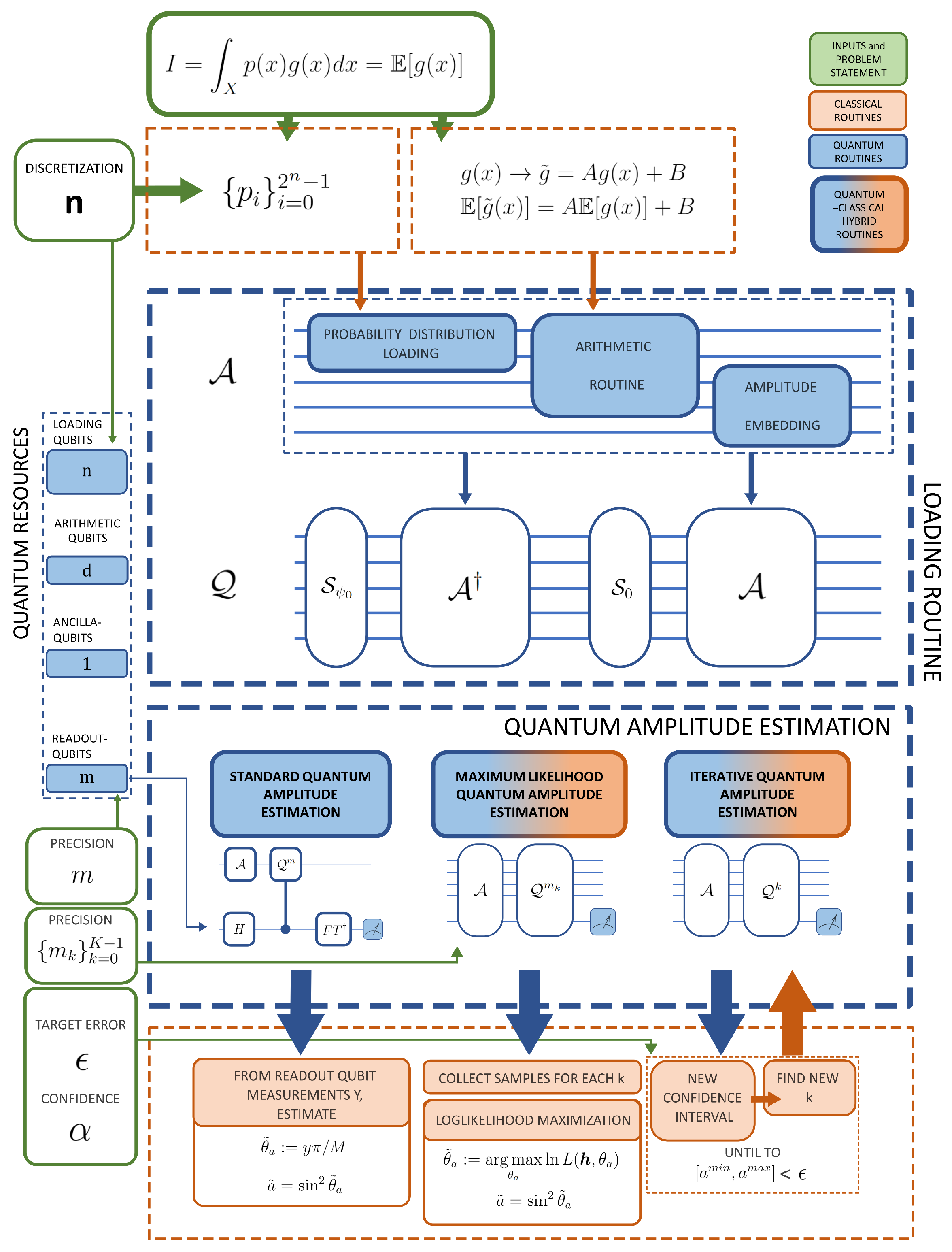
Flowchart of amplitude algorithms for integrals’ estimation. All the inputs of the algorithms are indicated in the green boxes, including the task of estimating the integral . The blue boxes, instead, represent the quantum routines, while the classic ones are in the orange boxes. The first step consists of choosing the discretization, which means how many qubits with which to load the probability distribution p. With n qubits, it is possible to encode values. The function can optionally be rescaled to obtain an integral and, then, rescale the expectation value in post-processing. The operators and its inverse , defined in Equation (3), are generally built in three steps: loading of the discretized distribution for which n qubits are needed, encoding of , for which d additional qubits are needed, via a routine for the necessary arithmetic calculations, and, finally, the embedding of the function , with the discretized values of x, to obtain the final state as in Equation (3). Once the operator has been obtained, it is possible to build the circuits necessary for the three QAE algorithms tested. The algorithms return the estimations of the integral and the confidential interval .
Figure 1.
Flowchart of amplitude algorithms for integrals’ estimation. All the inputs of the algorithms are indicated in the green boxes, including the task of estimating the integral . The blue boxes, instead, represent the quantum routines, while the classic ones are in the orange boxes. The first step consists of choosing the discretization, which means how many qubits with which to load the probability distribution p. With n qubits, it is possible to encode values. The function can optionally be rescaled to obtain an integral and, then, rescale the expectation value in post-processing. The operators and its inverse , defined in Equation (3), are generally built in three steps: loading of the discretized distribution for which n qubits are needed, encoding of , for which d additional qubits are needed, via a routine for the necessary arithmetic calculations, and, finally, the embedding of the function , with the discretized values of x, to obtain the final state as in Equation (3). Once the operator has been obtained, it is possible to build the circuits necessary for the three QAE algorithms tested. The algorithms return the estimations of the integral and the confidential interval .

Figure 2.
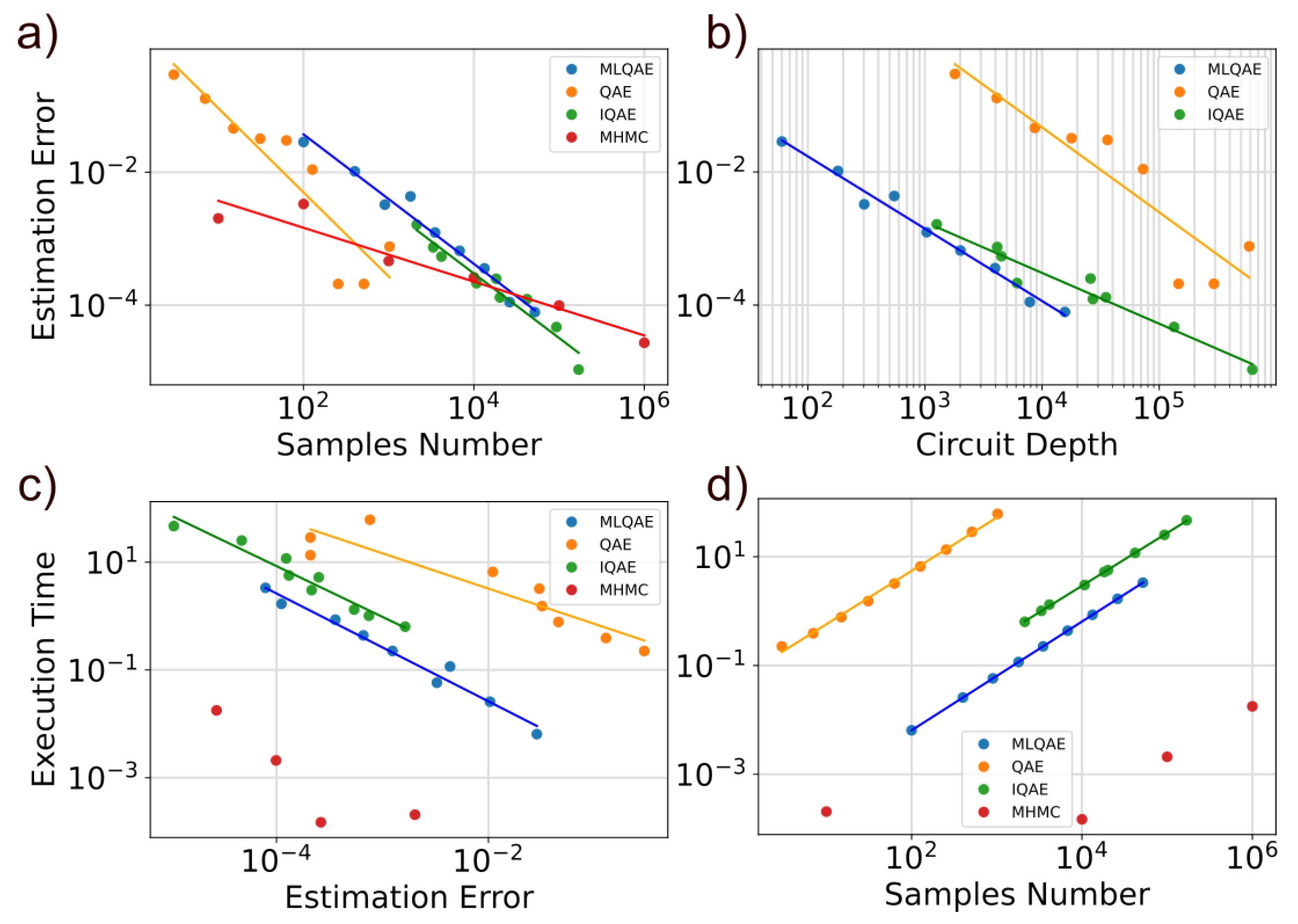
Performance of the amplitude estimation algorithms to estimate a 1D integral with qubits. All results of the quantum algorithms were obtained with the local Qiskit simulator ‘aer_simulator’, and each plot shows the average of 10 executions with different simulator seeds. All simulations of the IQAE [33] algorithm were performed with a 90% confidence interval. (a) The top-left plot shows how much the error in estimating the integral decreases as a function of the number of samples/oracle queries. The data are fit with a function in the log–log scale. For the algorithms MLQAE [32], standard QAE, IQAE, and classical Metropolis–Hastings Monte Carlo (MHMC), the slopes are, respectively, , , , and (a result obtained without considering the case with 10 samples). MLQAE and IQAE were performed with 100 shots per quantum circuit, while the QAE was executed as a standalone. The data showed a quadratic speed-up for the QAE (orange) and a slightly less-than-quadratic speed-up for the MLQAE and IQAE algorithms (blue and green, respectively) compared to the estimation using a classic sampling Monte Carlo method (red). (b) The top-right plot shows the estimation error as a function of the higher circuit depth (we must consider the highest one because MLQAE and IQAE require the simulation of more than one quantum circuit). The two lower plots, (c,d), show, instead, the execution time (for the quantum algorithms, it is the execution time of the QisKit local simulator) as a function of the estimation error (left) and the number of samples/oracle queries (right). In plot (d), the linear trends of the simulation times can be explained as follows: with the same number of qubits, the depth depends on the concatenated oracle queries , so the computing time linearly increases with the number of oracle queries.
Figure 2.
Performance of the amplitude estimation algorithms to estimate a 1D integral with qubits. All results of the quantum algorithms were obtained with the local Qiskit simulator ‘aer_simulator’, and each plot shows the average of 10 executions with different simulator seeds. All simulations of the IQAE [33] algorithm were performed with a 90% confidence interval. (a) The top-left plot shows how much the error in estimating the integral decreases as a function of the number of samples/oracle queries. The data are fit with a function in the log–log scale. For the algorithms MLQAE [32], standard QAE, IQAE, and classical Metropolis–Hastings Monte Carlo (MHMC), the slopes are, respectively, , , , and (a result obtained without considering the case with 10 samples). MLQAE and IQAE were performed with 100 shots per quantum circuit, while the QAE was executed as a standalone. The data showed a quadratic speed-up for the QAE (orange) and a slightly less-than-quadratic speed-up for the MLQAE and IQAE algorithms (blue and green, respectively) compared to the estimation using a classic sampling Monte Carlo method (red). (b) The top-right plot shows the estimation error as a function of the higher circuit depth (we must consider the highest one because MLQAE and IQAE require the simulation of more than one quantum circuit). The two lower plots, (c,d), show, instead, the execution time (for the quantum algorithms, it is the execution time of the QisKit local simulator) as a function of the estimation error (left) and the number of samples/oracle queries (right). In plot (d), the linear trends of the simulation times can be explained as follows: with the same number of qubits, the depth depends on the concatenated oracle queries , so the computing time linearly increases with the number of oracle queries.

Figure 3.
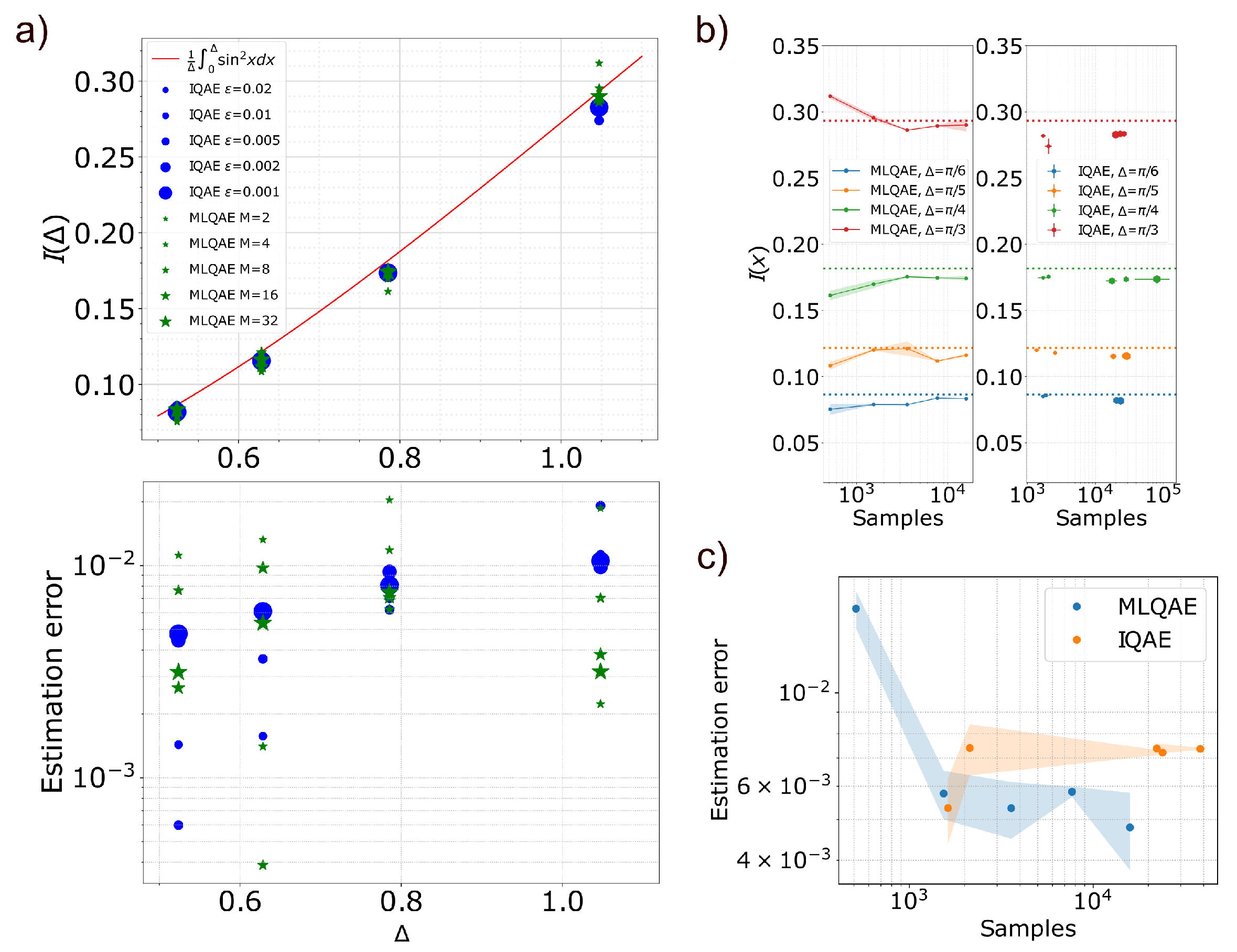
Performances of MLQAE and IQAE on the 11-qubit IonQ Harmony device. (a) Estimation of the integral function of Equation (15) at different values of , respectively set at , , , and . The blue dots represent the estimations obtained using the IQAE, while the green stars the MLQAE. The IQAE runs were performed at a confidence level of and . The size of the dots increases as the target error decreases. In the same way, the size of the stars increases as M increases in the MLQAE runs. Also, for the MLQAE runs, each circuit was repeated 512 times. Each dot and star represents the average of 5 different runs. The upper plot shows the fit of the results on the target function, and the lower plot shows the estimation errors reached by the two algorithms in different settings. (b) The two plots in this panel show how the estimation changes as the settings of the algorithms change for the four values of . The dotted lines represent the target values of the integrals . The right plot is for the MLQAE, and the left one is for the IQAE. For the MLQAE, the settings correspond to the number of samples represented on the x-axis. For the IQAE case, the results have an uncertainty on the number of samples, and the different settings are represented by the dot size. (c) The scaling of the estimation error with respect to the number of samples of both algorithms. Each dot is the average of all the runs (5 runs for 4 values of for a total of 20 runs). For the IQAE case, only the standard deviation of the estimation errors is shown.
Figure 3.
Performances of MLQAE and IQAE on the 11-qubit IonQ Harmony device. (a) Estimation of the integral function of Equation (15) at different values of , respectively set at , , , and . The blue dots represent the estimations obtained using the IQAE, while the green stars the MLQAE. The IQAE runs were performed at a confidence level of and . The size of the dots increases as the target error decreases. In the same way, the size of the stars increases as M increases in the MLQAE runs. Also, for the MLQAE runs, each circuit was repeated 512 times. Each dot and star represents the average of 5 different runs. The upper plot shows the fit of the results on the target function, and the lower plot shows the estimation errors reached by the two algorithms in different settings. (b) The two plots in this panel show how the estimation changes as the settings of the algorithms change for the four values of . The dotted lines represent the target values of the integrals . The right plot is for the MLQAE, and the left one is for the IQAE. For the MLQAE, the settings correspond to the number of samples represented on the x-axis. For the IQAE case, the results have an uncertainty on the number of samples, and the different settings are represented by the dot size. (c) The scaling of the estimation error with respect to the number of samples of both algorithms. Each dot is the average of all the runs (5 runs for 4 values of for a total of 20 runs). For the IQAE case, only the standard deviation of the estimation errors is shown.


Table 1.
Comparison between QAE algorithms. Here, is the number of qubits on which the oracle query is applied, d is the depth of , while is the target accuracy, and is the confidence level. In the last two algorithms, , , and . The types column indicates to which approach the algorithm belongs, based on the classification in Section 2.2: O corresponds to the original QAE, I to the MLAE approach, and II to the iterative approach, respectively.
| QAE Methods List | |||||||
|---|---|---|---|---|---|---|---|
| Algorithm | NISQ Readiness | Qubits | Depth | vs. | Speed-Up over MC | Ref. | Type |
| QAE | Low | ** | [10] | O | |||
| QAE NO-PE * | Medium | – | [32,41] | I | |||
| VarQAE * | High | – | [36] | I | |||
| Power-law QAE * | High | – | – | [37] | I | ||
| IQAE | Medium | Equation (12) | [33] | II | |||
| SQAE | Medium | – | – | – | [38] | II | |
| FAE | Medium | – | [40] | II | |||
* Classical optimization required; ** binomial distribution.
Disclaimer/Publisher’s Note: The statements, opinions and data contained in all publications are solely those of the individual author(s) and contributor(s) and not of MDPI and/or the editor(s). MDPI and/or the editor(s) disclaim responsibility for any injury to people or property resulting from any ideas, methods, instructions or products referred to in the content. |
© 2023 by the authors. Licensee MDPI, Basel, Switzerland. This article is an open access article distributed under the terms and conditions of the Creative Commons Attribution (CC BY) license (https://creativecommons.org/licenses/by/4.0/).
Share and Cite
MDPI and ACS Style
Maronese, M.; Incudini, M.; Asproni, L.; Prati, E. The Quantum Amplitude Estimation Algorithms on Near-Term Devices: A Practical Guide. Quantum Rep. 2024, 6, 1-13. https://0-doi-org.brum.beds.ac.uk/10.3390/quantum6010001
AMA Style
Maronese M, Incudini M, Asproni L, Prati E. The Quantum Amplitude Estimation Algorithms on Near-Term Devices: A Practical Guide. Quantum Reports. 2024; 6(1):1-13. https://0-doi-org.brum.beds.ac.uk/10.3390/quantum6010001
Chicago/Turabian StyleMaronese, Marco, Massimiliano Incudini, Luca Asproni, and Enrico Prati. 2024. "The Quantum Amplitude Estimation Algorithms on Near-Term Devices: A Practical Guide" Quantum Reports 6, no. 1: 1-13. https://0-doi-org.brum.beds.ac.uk/10.3390/quantum6010001