On the Generation of Harmonics by the Non-Linear Buckling of an Elastic Beam


CCTAE, IDMEC, LAETA, Instituto Superior Técnico, Universidade de Lisboa, Av. Rovisco Pais 1, 1049-001 Lisboa, Portugal
*
Author to whom correspondence should be addressed.
†
These authors contributed equally to this work.
Appl. Mech. 2021, 2(2), 383-418; https://0-doi-org.brum.beds.ac.uk/10.3390/applmech2020022
Submission received: 21 March 2021
/
Revised: 30 May 2021
/
Accepted: 7 June 2021
/
Published: 15 June 2021
(This article belongs to the Special Issue Mechanical Design Technologies for Beam, Plate and Shell Structures)
Abstract
:The Euler–Bernoulli theory of beams is usually presented in two forms: (i) in the linear case of a small slope using Cartesian coordinates along and normal to the straight undeflected position; and (ii) in the non-linear case of a large slope using curvilinear coordinates along the deflected position, namely, the arc length and angle of inclination. The present paper starts with the exact equation in a third form, that is, (iii) using Cartesian coordinates along and normal to the undeflected position like (i), but allowing exactly the non-linear effects of a large slope like (ii). This third form of the equation of the elastica shows that the exact non-linear shape is a superposition of linear harmonics; thus, the non-linear effects of a large slope are equivalent to the generation of harmonics of a linear solution for a small slope. In conclusion, it is shown that: (i) the critical buckling load is the same in the linear and non-linear cases because it is determined by the fundamental mode; (ii) the buckled shape of the elastica is different in the linear and non-linear cases because non-linearity adds harmonics to the fundamental mode. The non-linear shape of the elastica, for cases when powers of the slope cannot be neglected, is illustrated for the first four buckling modes of cantilever, pinned, and clamped beams with different lengths and amplitudes.
1. Introduction
The Bernoulli [1] and Euler [2] theory of beams is a standard introductory subject in textbooks on elasticity [3,4,5,6,7,8,9,10,11] and leads to the phenomenon of buckling, which has been considered in several conditions: (i) geometric and material non-linearities [12]; (ii) in combination with shear [13,14] that is more significant for thin-walled beams [15,16,17,18,19]; (iii) constraints [20,21,22], such as hyper or non-local elasticity [23,24]; (iv) vibrations [25,26], that can be excited by unsteady applied forces [27,28,29,30,31,32,33], leading to control problems [34]; (v) steady mechanical [35] or thermal [36,37,38] effects; and (vi) vibrations of tapered beams [39,40,41,42,43,44,45,46,47,48,49,50,51,52,53,54,55], with multiple applications like airplane wings and flexible aircraft and helicopters [56,57,58,59,60,61,62,63,64]. Among this wide range of topics related to the buckling of elastic beams, the present paper focuses on geometric non-linearities associated with a large slope of the elastica.
The equation of the elastica of a beam is usually written in one of the two forms: (i) in Cartesian coordinates,
with the x-axis along the undeformed beam; or (ii) in curvilinear coordinates,
with the arc length s as a function of the angle of inclination. The linear theory assumes for (1a) a small slope,
where the prime in this paper denotes the derivative with x, and implies that the maximum deflection is small, compared with the length (Figure 1),
However, the latter condition of small maximum deflection relative to length (2b) does not imply [65] linearity (2a) in the case of “ripples” with a large slope (Figure 2). The condition of linearity can be expressed in terms of a small angle of inclination,
that is equivalent to
The Euler–Bernoulli theory of beams states that the bending moment M is proportional to the curvature k,
that is the product of the Young modulus E of the material by the moment of inertia I of the cross-section. For a beam of constant cross-sections made of a homogeneous material, the bending stiffness is constant. In the case of a uniform beam [66], that is, with constant bending stiffness, geometric non-linearities can arise from the curvature, ,that is, the rate of change of the angle of inclination with the arc length
The curvature is given by
and thus, it is only in the case of a small slope (2a) that the equation of the elastica is linear:
If the slope of the elastica is not small, its shape is specified by non-linear ordinary differential equations [67,68,69,70,71,72,73,74,75,76,77,78,79].
The linear theory shows that if a critical buckling load is reached, a beam in the tension deforms and gains a buckled shape, and higher critical loads, with , lead to a succession of harmonics . In the present paper, it is shown that geometric non-linearities associated with a large slope,
do not affect the critical buckling load, but change the shape of the elastica that becomes a superposition of harmonics of the linear case,
The coefficients are determined in this paper for the three cases of (i) cantilever, (ii) clamped, and (iii) pinned beams, and the shape of the elastica is illustrated taking into account non-linear geometric effects associated with a large slope. Before proceeding to discuss non-linear geometric effects in the Euler–Bernoulli theory [1,2,3,4,5,6,7,8,9,10,11], the preceding classification of the references [12,13,14,15,16,17,18,19,20,21,22,23,24,25,26,27,28,29,30,31,32,33,34,35,36,37,38,39,40,41,42,43,44,45,46,47,48,49,50,51,52,53,54,55,56,57,58,59,60,61,62,63,64] is complemented by a brief discussion of some additional references. The method of the elastica for non-linear beams, schematized in Figure 3, involves the solution of ordinary differential equations [66,67,68,69,70,71,72,73,74,75,76,77,78,79]. The exact analytical solutions can be obtained using elliptic functions [80,81,82,83,84,85] for simpler loading cases.
The articles [86,87] show that large deflections are specified by a combination of incomplete and complete elliptic integrals. The results of these two articles are given with limited accuracy, because at that time, the calculations were not performed with digital computers. More accurate results of elliptic integrals are presented, for instance, in [88,89]. Furthermore, to obtain highly accurate numerical results, these problems may also be solved using the shooting-optimization technique. The aforementioned two methods for solving large deflections of beams are presented in [90], where an inextensible elastic beam is hinged at one end, while the other end is assumed to be a frictionless support where the beam can slide freely. Additionally, the beam is under a moment gradient and the moment at each end of the beam can be varied from zero to a full moment by a scaling parameter. In [90], the elastica theory serves to formulate the elliptic-integral method, and the results are obtained by an iterative process, while the governing set of differential equations are needed for the shooting-optimization technique and are numerically integrated using the fourth-order Runge–Kutta method. The results obtained from both methods are in close agreement to each other. The paper [91] continues in this line of research, but considers the double curvature bending of the elastica under two applied moments in the same direction applied at the supports, and complements earlier studies that confined bending to one of the single curvature-type bendings. The two aforementioned methods are used. The elliptic integral technique provides analytical solutions to the governing non-linear differential equation for elasticas, while the shooting optimization method numerically integrates the equation using the fifth-order Cash–Karp Runge–Kutta method. Both methods provide almost the same stable and unstable equilibrium solutions and, for some cases of the unstable equilibrium configuration, the elastica can form a single loop or snap-back bending.
Continuing in this line of investigation, the paper [92] considers the large deflection problem of variable deformed arc-length beams, also with a uniform flexural rigidity, but under a point load. In [92], the ends are partially elastically supported against rotation (it covers both the cases of hinged or clamped ends). Both previously mentioned methods are also used, and the results obtained are in close agreement. This kind of problem highlights the possibility of two equilibrium states for a given load, implying the possibility of a snap-through phenomenon, the existence of a critical load, and a maximum arc-length for equilibrium. The analytic elastica solution of slightly curved cantilever beams, fixed at one end, while being deflected under couples and forces of various directions, is evaluated in [93] using elliptic integrals. It has been shown that for some cases, the solution is very sensitive to small errors in the calculation of elliptic integrals. An analytic elliptic solution for the post-buckling response of a linear-elastic and hygrothermal beam, subjected to an increase in temperature and/or moisture content, is presented in [94]. In [94], the beam is pinned at both ends, and therefore the extensibility of the beam cannot be ignored. Additionally, it shows that the critical load is a maximum and, in the post-buckling regime, the magnitude of the load decreases. The beam theory can be extended to more complex structures [95].
Other methods using the elastica approximation are useful for more complex loadings. The paper [96] determines a parametric solution to the elastic pole-vaulting problem, where the pole is taken to be a thin uniform elastic column with the upper end being subjected to lateral and transverse forces and a bending moment at the same time as the bottom end is free to pivot during the vaulting. The parametric solution is given in terms of tabulated elliptic integrals. The investigation [97] gives a closed-form solution for the problem of a non-linear elastica and buckling analysis of a straight bar, due to concentrated and uniformly distributed loads, while the flexural rigidity varies along the bar. It achieves an integral closed-form solution of the equation governing the equilibrium of the bar, by applying successive functional transformations. The paper [98] presents the buckling analysis of an elastic continuous bar on several rigid supports subjected to end-compressive forces, and assumes that the compressive forces and flexural rigidities vary from one span to the next. The closed-form solution expressed by elliptic integrals is derived for each span. The same authors presented an analytic solution for the problem of non-linear elastic buckling of a straight bar subjected to bending compression due to forces and couples at the ends superimposed to a uniformly applied transverse load along its length in [99], by applying functional transformations. Additionally, the same authors analysed the problem of non-linear buckling for a straight uniform bar, fixed at its base and free at its upper end, due to the bar’s own weight in [100]. It yields reliable results in agreement with the physical problem. The same procedure was used in [101] to study the problem of non-linear buckling for a straight bar of uniform cross-sections and flexural rigidity, lying on a continuous elastic medium, and subjected to terminal point-loads and bending moments. In all the works described above, the effects of transverse deformation due to axial, lateral, and transverse forces are negligible.
The paper [102] constructs an exact parametric analytic solution for the full non-linear differential equations of the cantilever elastica due to end loads, end couples, and also including the effects of transverse deformation, completing, for instance, the work [96]. Translational or rotary springs may be used [103] to brace a beam increasing its critical buckling load, or to have the opposite effect of decreasing the critical buckling load to facilitate demolition. The buckling can also be facilitated or opposed by supporting the beam on a continuous bed of springs [66]. A beam of variable cross-sections can taper in two directions [104], for example, in the case of a pyramidal beam representing an airplane wing with chords much larger than the thickness affecting the natural frequencies of bending modes.
Following this introduction (Section 1) to the Euler–Bernoulli theory of beams, the core of the paper focuses on geometric non-linearities associated with a large slope of the elastica. The equation of the elastica of a uniform beam (Section 2) is obtained without restriction on the slope of the elastica (Section 2.1). The well-known solutions for the linear case of a small slope are briefly recalled (Section 2.2) because they supply the harmonics for non-linear corrections (Section 2.3). The linear and non-linear cases are also compared, as concerns the boundary condition with small and large slopes, respectively, at the free end of a cantilever beam (Section 2.4). The cantilever beam is considered first (Section 3) to obtain the non-linear shape of the elastica (Section 3.1) and to compare the linear approximation with non-linear corrections of all orders (Section 3.2). The non-linear effects on the shape of the elastica are illustrated using the representation as a superposition of linear harmonics, by truncating the series in an analytic approximation (Section 3.3), and adding a larger number of terms in a numerical computation (Section 3.4). The non-linear buckling is also considered for clamped and pinned beams (Section 4), starting with the non-linear effects of a large slope (Section 4.1), that do not affect the critical buckling load (Section 4.2), but do change the shape of the elastica by the generation of harmonics (Section 4.3), illustrated by numerical calculations (Section 4.4). The conclusion (Section 5) highlights the use of linear buckling harmonics to specify the shape of the elastica for non-linear buckling with a large slope.
2. Non-Linear Bending of a Beam with Large Slope
The non-linear bending of a beam with a large slope is considered to specify the relation between the axial tension, bending moment, and transverse force or shear stress (Section 2.1). The resulting equation of the elastica is solved readily in the linear case of a small slope (Section 2.2), specifying the harmonics to be used in the non-linear case (Section 2.3). The linear and non-linear cases of small and large slopes, respectively, are also compared, as concerns the boundary condition at the free end of a cantilever beam (Section 2.4).
2.1. Bending Moment, Transverse Force and Shear Stress
The transversal distributed and punctual forces F at the end sections, with the longitudinal tension T, cause a bending moment M (denoted in the Figure 4). The variation of the bending moment along the arc length of the elastica is balanced by the transverse force F, plus the vertical component of the tangential tension T:
The tangential tension and its vertical component are related (Figure 5) by
where is the vertical displacement. Substitution of the last equation in (10b) yields the balance of bending moment, transverse force and tangential tension:
Using (4), which has the minus sign because the y axis points downwards, leads to: (i) the transverse force equal to
(ii) the shear stress defined by the transverse force per unit length
Substituting (5) and (8) in (10c), it follows that the transverse force is related to the shape of the elastica by
and (12) leads to the relation between the shear stress and the shape of the elastica by
The case considered in this paper is of uniform axial tension,
and constant bending stiffness
A constant bending stiffness (15b) applies: (ii-a) to a homogeneous beam with uniform cross-section ; or (ii-b) to an inhomogeneous beam whose Young modulus varies along the length inversely to the moment of inertia of the cross-section. Since buckling occurs only for axial compression , the buckling parameter p is defined by
and has the dimensions of inverse length. It is real for a compression when because ; otherwise, it is imaginary for a traction with because . For a uniform beam, the buckling parameter p is constant because and T are also constants for that case.
Simplifying the Equation (13) for a uniform beam, the buckling parameter appears in the transverse force, specifically in the form
It is the first fundamental equilibrium equation for a uniform beam. Simplifying the Equation (14) for the same type of beams, the buckling parameter also appears in the shear stress expression, in the form
It is the second fundamental equilibrium equation for a uniform beam. In both equations, there are two different types of linearity: (i) all terms are non-linear with respect to the slope of the elastica , given by (2a); (ii) one term is linear if the sine of the angle of inclination is used as a variable,
The curvature (6) is related to (18a) by
that is a non-linear function of the slope of the elastica. Thus, the equation of the elastica for the transverse force F is: (i) of the third order in terms of the shape of the elastica and has all non-linear terms in (16a); (ii) of the second order involving some terms linear with an auxiliary variable in (16c), namely, the sine of the angle of inclination whose derivative is exactly the curvature k, as indicated in (18b). Furthermore, the equation of the elastica for the shear stress f is: (i) of the fourth order in terms of the shape of the elastica and has all non-linear terms in (17a); (ii) of the third order involving some linear terms with the sine of the angle of inclination in (17c). Thus, the non-linearity does not lie entirely in the auxiliary variable , and is preferred to solve the non-linear differential equation in terms of , since the degree of the equation is reduced by one.
The bending moment can be evaluated, again, as a function of or as a function of . The linear case of a small slope is reviewed briefly, in Section 2.2, for comparison with the non-linear case of a large slope, that is the main focus of and occupies the remainder of the paper.
2.2. Linear Buckling for Small Slope
The linear bending corresponds to the small slope (2a) and leads to the following consequences: (i) the angle of inclination of the elastica in (18a) simplifies to
where the inclination is equal to the derivative of deflection of the beam; (ii) the curvature k of the elastica, from (18b), simplifies to
(iii) the simplification of the curvature leads to the bending moment
To deduce the last three equations (the constitutive and equilibrium equations), the only simplification regarded was to consider linear bending, and thence they can be applied to any type of beam (for instance, it is not necessary to be uniform).
In the case of linear deflection, when (2a) is taken into account, and simultaneously of a uniform beam, when the Equation (15a,b) are considered (again, when it is valid the assumptions and ), the transverse force and shear stress simplify further, respectively, to
The beam is elastically stable if, and only if there is no deflection in the absence of shear stress. Otherwise, the beam is elastically unstable if, and only if there is deflection in the absence of shear stress. For a uniform beam, considering again the assumptions that T and are both constants, in the absence of shear stress, , instability is possible only if the buckling parameter is positive, , in (17c), that is, under compression , corresponding to
and leading to the linear differential equation of fourth order with constant coefficients
for the shape of the elastica, whose solution is
where , , and are the four arbitrary real constants. However, there is also a fifth indeterminate constant, namely, the buckling parameter p, that is intrinsically related to the critical axial tension.
For subsequent comparison with the non-linear theory, two sets of well-known results are quoted from the literature [3,4,7,66] on linear buckling of beams: (i) firstly, the critical buckling load, that is, the magnitude of the compressive axial load at the onset of buckling, is highest for a clamped beam,
lowest for a cantilever beam,
and for a pinned beam, the value is in between, because
(ii) secondly, the shape of the buckled elastica in the linear approximation is, respectively, for the clamped, for the pinned, and for the cantilever cases, given, respectively, by
where the arbitrary real constant b is an amplitude, and L is the length of the beam. The last results are deduced for the fundamental mode of buckling, that is, for the lowest possible value of T that buckles the beam. The linear results will be compared in the sequel with the lowest-order non-linear theory in the next subsection. The fundamental mode shapes of the buckled elastica using the linear approximation are plotted in the Figure 6.
2.3. Lowest-Order Non-Linear Buckling for Large Slope
In the linear case of a small slope without forcing, the elastica satisfies a linear differential equation with constant coefficients of fourth order for the transverse displacement, as stated in the Equation (22b). However, in the non-linear case of a large slope without forcing, regarding the definition (18a) that is equivalent to
used to derive the non-linear variable as a function of , the elastica satisfies a non-linear differential equation with constant coefficients of order three, using the Equation (17c) with ,
using the sine of the angle of inclination as a dependent variable that is non-linear. The last two expressions are valid for small or large deflections and can be linearised for small deflection, as in the Section 2.2. However, although the relation (25a) is valid for any type of beam because it is a definition, the Equation (25b) is only correct for uniform beams, in the absence of shear stress (to study the buckling phenomenon). Indeed, only uniform beams will be studied in the remainder of this paper, and therefore, the comparison between different theories will be made only for that type of beams.
The differential Equation (25b), for
because the beam is uniform, has a first integral
where A is an arbitrary constant. Re-arranging the last expression in the form
it can be integrated (p. 500 of [105]) as
where B is another arbitrary constant. The last equation is still exact for a uniform beam without shear stress. Henceforth, there are two distinct approximations that can be done. The linear approximation of a small slope (2a) implies in (18a). Otherwise, the lowest-order non-linear approximation implies
and if it is applied to (26d), then it results in
using only the leading terms of the power series for the square root or binominal (p. 384 of [65]) and for the arc of circular sine (p. 508 of [84]). The integration of (27b) introduces another arbitrary constant C in
which relates to the sine of the angle of inclination with the longitudinal coordinate of the beam, and is valid only for the lowest-order non-linear approximation (27a) and for the uniform beam (15a,b).
The shape of the elastica, derived without any simplification, is given by the definition (25a) involving another constant of integration D in
Thus, in the linear case of a small slope (2a) and for a uniform beam, the shape of the elastica is given by (22c), while otherwise, in the lowest-order non-linear approximation (27a) also for a uniform beam, the shape of the elastica is given by (27c) and (28), in both cases involving four arbitrary constants plus the indeterminate value p. The four boundary conditions, two at each end of the beam: (i) specify three constants in terms of one, that is an arbitrary amplitude; and (ii) determine the eigenvalues p, of which the smallest specifies the critical buckling load, according to the definition (15c). It will be investigated in the sequel whether (i) the critical buckling load and (ii) the shape of the elastica are equal or different in the linear and non-linear cases of small (2a) and moderate (27a) slopes, respectively. This will be ascertained by considering three classical cases of support by order of increasing critical buckling load, namely: (i) cantilever beam in the Section 3; (ii) pinned and clamped beams, both in Section 4. In the case (i) of the cantilever beam, there is a boundary condition at the free end that is compared next (Section 2.4) in the linear and non-linear cases of small and large slopes, respectively.
2.4. Linear and Non-Linear Boundary Conditions at a Free End
A cantilever beam, represented in the top-left scheme of the Figure 6, is clamped at one end, and free at the other end. Four boundary conditions must be known to evaluate the critical buckling load and the shape of the elastica. For a cantilever beam, the bending moment at the end of the beam is zero, , and the transverse force must also vanish at that point, . To obtain the force boundary condition at the free end, the Equation (16a–c) are used. The two aforementioned boundary conditions, regarding (16c) and (19) respectively, lead to the non-linear boundary conditions in terms of
In the linear case of a small slope (2a), the boundary conditions become
On the other hand, in the non-linear case of an unrestricted slope, the free-end boundary condition of a zero-bending moment (19) is in terms of the sine of the inclination of the elastica
or, regarding (18a), in terms of the displacement of the elastica
The free-end boundary condition of transverse force, again (16c) with (25a) for the case of an unrestricted slope, is
or in terms (16a) of the displacement of the elastica
The passage from (31a) to (31b) uses the Equation (18a), while the passage from (32a) to (32b) uses the next relation
The boundary conditions for the displacement at the free end in the linear and non-linear cases of small and unrestricted slopes, respectively, of a uniform beam (when the Equation (15a–c) are valid): (i) coincide for the vanishing of the bending moment because (30a)=(31b); (ii) however, do not coincide for the transverse force because (30b)≠(32b), since the second term in (32b) differs from the first term in (30b).
3. Non-Linear Buckling of a Cantilever Beam
The non-linear equation of the elastica is integrated first for a cantilever beam (Section 3.1) specifying the linear approximation (in agreement with Section 3.2). The non-linear corrections are considered analytically for the lowest-orders (Section 3.3) and numerically for higher orders (Section 3.4).
3.1. Non-Linear Elastica of a Cantilever Beam
The first integral of the differential equation for the elastica is (26b), arising from the integration of (25b), that is valid only for a uniform beam (and therefore the parameter p is constant because T and are also constants); however, it can be applied not only for linear, but also for the non-linear case. It involves a constant A and is rearranged in the next form:
In the case of a cantilever beam, the transverse force must vanish at the free end, leading to the boundary condition (29b). Comparing to the last expression, then , or . Consequently, the last condition simplifies the second integral (26d). Henceforth, in this section, the results are deduced with the lowest-order non-linear approximation (27a). With this approximation, the Equation (27c) with simplifies to
involving the constant
The primitive (35a) can be written in the form
Up to this point, two assumptions were used: uniform beam and lowest-order non-linear approximation. The clamping boundary condition at the fixed end, (the slope of the elastica at that point must be zero), from (18a) which is an exact relation, implies , and hence,
leading to the second result from the boundary conditions,
One could set to verify the last boundary condition, but in that case, would be equal to zero along the beam, and we are interested only in non-zero solutions of and . Substituting (37b) in (36) and introducing another arbitrary constant,
lead to
In spite of being valid, the more general solution of the last boundary condition would be , and consequently, . However, in that case, the successive buckling loads and the shape of the elastica are the same as setting , which is simpler. The boundary condition stating that the bending moment vanishes at the free end, , repeated here for convenience, is in the non-linear case, and applied to (38b), we have
that leads to
Thus, the successively buckling loads that make the beam unstable are
where the first subscript 3 stands for the cantilever case, and the second subscript n stands for the n-th mode of the buckling.
Consequently, the critical buckling load is evaluated with the lowest possible value of the buckling parameter, and it is equal to
which is the same in the linear (23b) and lowest-order non-linear (39d) cases for a cantilever beam that is free to move at the free end. Knowing the sine of the slope of the elastica , the non-linear slope is obtained substituting (38b) in the exact kinematic relation (25a):
To compare with the linear case, a relation between the constant G and another constant from the linear results is needed. In the linear case, , the factor with the square root can be omitted. Then, the Equation (40) in the linear case concerning the first mode of buckling (the results for this mode are shown in the Section 2.3) leads to
In agreement with the linear result (24c), the arbitrary constants G and b are related by
but generally, the relation must be .
In the non-linear case, the square root in (40) cannot be omitted. The assumption that the slope does not exceed unity, , leads, considering the exact relation (18a), to
and thus, the inverse square root in (40) can be expanded (p. 384 of [84]) in a binomial series
with coefficients
The double factorial is used in the coefficients, and its definition with some properties are reviewed in the next equations:
The first seven coefficients are indicated in Table 1.
The Equation (44) applies for , and . Thus, the slope of a uniform cantilever beam under axial compression is given by substituting the Equation (43) in (40) that is equivalent to
The leading term is the linear slope (deduced from the linear approximation) by comparing the last result with the Equation (41a). The following terms (Table 1) are non-linear corrections of increasing order. Furthermore, the displacement can be obtained by integration of (46), and thus consists of the lowest-order linear approximation plus non-linear corrections of all orders that are evaluated next. At this point, in spite of having four boundary conditions for a cantilever beam, only three of them were used: the bending moment vanishes at , the transverse force also vanishes at the same position, and the derivative of the elastica (its slope) at the beginning of the beam is zero.
3.2. Linear Approximation and Non-Linear Corrections of All Orders
There is one last boundary condition that was not used yet: the beam is fixed at its beginning, and hence, the transversal displacement at that point is zero, . Integrating the Equation (46), the displacement is given by a sum,
of terms
Note that in the Equation (47a), there is no arbitrary constant of integration that is equal to zero, because of the boundary condition . Therefore, at this point, all four boundary conditions were used. The zero-order term is the linear approximation
where (39d) and (41b) were used to prove the third and fourth equalities successively in agreement with (24c). The lowest-order non-linear correction is
where the value of , indicated in Table 1, and some elementary trigonometric relations [105] were used in the determination of .
The two lowest-order terms in (47a) have been evaluated explicitly in (48) corresponding to the first term, and (49) corresponding to the second term, in the case of a lowest-order non-linear approximation . To estimate the error of the truncation of the series (47a), the higher-order terms in (47b) may be considered. In order to explicitly evaluate the m-th order, the expansion of the odd power of sine (p. 335 of [105]) is used as a sum of sines of multiple angles:
Substituting the last expression in the m-th order, the non-linear correction (47b) becomes
it can be confirmed that substituting and in the last expression leads, respectively, to (48) and (49). The maximum deflection at the tip, considering the fundamental mode of buckling and regarding (39d), is given by
that relates the constant G to the maximum deflection.
3.3. Truncation of the Series in the Shape of the Elastica
The exact shape of the buckled cantilever beam is given by the sum of the series (47a), having infinite terms. The series converges when and diverges when . Therefore, is a necessary condition to evaluate the series (47a). To obtain accurate results, only the first terms need to be evaluated, and m can be small. The Table 2 shows the number of iterations (the number of terms of the series) needed to calculate the sum (47a) with absolute and relative errors smaller than ; that is, the iterations stop when the difference between two consecutive terms, and , is smaller than , and when the ratio between that difference and the last term evaluated is also smaller than . To have an error with such a small order of magnitude, few terms are needed, for instance, with respect to the fundamental mode of buckling (with , for a beam with length , only the first 10 terms are needed). Furthermore, one can conclude that the number of iterations is intrinsically related to the value G for each case. When G becomes closer to 1, which is the boundary of convergence of the series, more iterations are needed to converge with the same error. For instance, looking at the data of Table 2, the case when more iterations are needed is when and , because it is the case when G is closest to 1. The parameter G is equal to . Consequently, for the same parameter b, more iterations are necessary to obtain accurate results for shorter beams and for higher modes of buckling, corresponding to larger slope and stronger non-linearity, as highlighted in Table 2.
One specific example of the non-linear theory of buckling is illustrated next in the case of a cantilever beam, for which the linear approximation to the shape of the elastica (47a) is just the first term of the sum, substituting in (51), or equivalently, the result (48). However, the exact shape using the lowest-order non-linear approximation is given by the infinite sum in (47a), and the Table 2 highlights that when G is close to 1, the number of necessary terms increases very rapidly, possibly requiring a larger computational effort to obtain accurate results. Therefore, in the case of an arbitrary amplitude, the value , that satisfies (42) being close to the limit, is chosen to understand if the shape can be deduced with very few terms. The linear approximation () of the shape of the elastica is
The dimensionless variables and are used for plotting the successive iterations of the sum (47a) in the Figure 7, to make the results not dependent on the explicit values of the order of buckling n and the length L. Considering now the non-linear terms, the corresponding lowest-order non-linear correction () is
that is also plotted in the Figure 7.
The total non-linear deflection of the buckled cantilever beam, using the lowest-order non-linear approximation (also plotted in the Figure 7), shows that the maximum deflection of the fundamental mode of buckling, that occurs at , is
in the linear approximation, to which the first non-linear correction adds , leading to the total value
The linear approximation (53), over its whole length, , leads to a monotonic shape of the elastica because
The lowest-order non-linear correction (54) is also monotonic, since
thus increasing the deflection everywhere, and consequently, the maximum deflection is at the end of the beam. It is at that point where the difference between the linear approximation and the lowest-order non-linear correction is at its maximum.
The non-linear corrections of all higher orders (47a) are specified by (51), including the maximum deflection at the tip (52), and since they go beyond the hypothesis , they serve only as order-of-magnitude estimates of the error caused by truncating the non-linear series after the first non-linear term. The second-order non-linear correction, setting in (51), would introduce the factor multiplied by a term, giving the result of order , that is a correction of less than 2% compared with (55b). This would be hardly visible in the plot of the Figure 7 that is limited to the sum of the linear approximation (53) plus the lowest-order non-linear correction (54). Thus, the buckled shape of a cantilever beam, for , is given exactly by (51) to all orders in the amplitude G, with the lowest-order non-linear approximation consisting of the linear approximation (48) and lowest-order non-linear correction (49). The higher-order terms go beyond the approximation and apply only as an indication of the order of magnitude of the error due to stopping at the lowest-order non-linear correction; for example, the order of magnitude of the lowest-order non linear approximation is sufficient, summing (53) with (54) in the case to obtain the shape of the elastica using only the first two iterations (Figure 7) with less than 2% in the accuracy error.
The non-linear shape of the buckled elastica in the post-buckling regime can be represented as a superposition of harmonics of the elastica in the linear approximation. In the case illustrated of a cantilever beam with moderate non-linearity, the buckled shape is approximated by a superposition of the fundamental and first harmonic with a suitable ratio of the amplitudes of the two terms, calculated using the method detailed in this paper.
3.4. Numerical Results for the Buckling of a Cantilever Beam
The Figure 8, Figure 9 and Figure 10 are obtained using many more iterations of the series (47a) than the first two terms; they are obtained with 30 terms, that is, calculating the first 30 terms of the series, to obtain more accurate results, although the difference is not as significant as using only the first two terms. The figures show a solution for each case of the differential equation that specifies the shape of the elastica of a cantilever beam. To obtain the solution, it was assumed that ; however, a more general condition would be , leading to with . The plots of the figures are obtained with , but one can assume , meaning that is also a valid solution, and consequently, . Therefore, and are the two possible solutions for each case (in the plots, only one of them is sketched), meaning that the beam can buckle on one side or on the opposite side with equal probability.
The Figure 8 shows the effect of varying the indeterminate real constant b on the several mode shapes of the buckled elastic cantilever beam for the first four orders of buckling. The constant b only serves to obtain numerical results of and does not influence the shape of the elastica. The effect of b is only on the magnitude of the elastica, not altering the positions of maximum and minimum deflection of the beam. These observations are valid independently of the order n and length of the beam L. For the fundamental mode of buckling, the shape of the beam increases monotonically, leading to a maximum amplitude at the tip, and for higher modes of buckling, the shape oscillates along the beam, leading to alternate peaks and nulls of the oscillation. Increasing the order n leads to more peaks and nulls because the period of the trigonometric functions is shorter.
The effect of length L on the shapes of the buckled elastic cantilever beam for the first four orders of buckling is shown in the Figure 9. Changing the length L does not significantly influence the values of maximum deflection, although this effect is more significant for higher modes of buckling. For longer beams, the maximum deflection of the buckled beam is lower. The reason is because according to the Equation (51), each term of the series (47a) is proportional to , and consequently, is proportional to . The length L has a more significant effect in the positions of maximum deflection of the beam. While L is increasing, the period of the sine functions also becomes longer, and therefore, looking at the plots of Figure 9 in a down-top approach, one can conclude that the first maximum occurs for the shorter beam, while the last maximum occurs for the longer beam.
In the Figure 10, the difference between the linear approximation () and the higher-order terms of the non-linear approximation () is shown for several lengths and for the first four orders of buckling. The linear approximation is less accurate for shorter beams and for higher orders of buckling. It is the same conclusion of Table 2. According to the Table 2, more iterations are needed for shorter beams and for higher values of n, and therefore, the difference induced by the non-linear terms of the series (47a) is higher for these cases. A shorter beam and higher-order modes lead to “ripples” with a large slope (see Figure 2), and thus, larger non-linear effects. Furthermore, the maximum difference between the two levels of approximation occurs at the extreme amplitudes of the deformation of the beam, independently of the parameters n and L. The maximum difference therefore occurs when the derivative of is zero, and is again more noticeable for shorter beams and higher values of n. For the fundamental mode of buckling (), the difference is negligible, and therefore, one can use the linear approximation to obtain accurate results. Moreover, comparing the two approximations, the beam buckles more when the lowest-order non-linear approximation is used than the linear approximation; that is, for the same axial tension and parameters of the beam, the value of the deflection obtained with the linear approximation is lower than with the non-linear approximation. Consequently, the linear approximation underestimates the strength of the buckling loads, and the rigidity of the beam appears to be higher in this case.
4. Non-Linear Buckling of Clamped and Pinned Beams
The lowest-order non-linear theory of buckling (Section 4.1) applies not only to a cantilever beam (Section 3), but also to clamped and pinned beams (Section 4.2), showing that in all cases, the critical buckling load is the same as in the linear case (Section 4.3), but the shape of the buckled elastic is not due to the generation of linear harmonics, that is illustrated numerically (Section 4.4).
4.1. Non-Linear Effects of Large Slope
The critical buckling load for a cantilever beam was shown to coincide in the linear (23b) and lowest-order non-linear (39d) cases. Two possible explanations are that: (i) a cantilever beam can move at the free end; or (ii) the buckling is a linear phenomenon, and thus its onset is not affected by non-linear effects. The first explanation (i) can be tested by determining the critical buckling load of non-cantilever beams using the lowest-order non-linear theory. For a non-cantilever beam, the simplification does not hold, because is not a boundary condition for pinned nor clamped beams. In the Equation (27c), valid for uniform beams and simultaneously using the lowest-order non-linear approximation, the argument of the square root is written as
The constant G is now defined by
so that in the case of a cantilever beam, and then G coincides with the earlier definition (38a), and in (58) appears the square of a new dependent variable
Inverting (60) and using the new variables (59a,b) specifies the sine of the slope, given by
and specifies the respective curvature and the bending moment, using (18b), given by
with amplitudes
The three arbitrary constants (A, B, C) may be replaced by (H, G, C), and the Equation (61a–d) are valid for uniform clamped and pinned beams, considering the lowest-order non-linear approximation. Although H and G can simultaneously be zero, would also be equal to zero and be a valid solution, but we are interested in only non-zero solutions of and .
4.2. Coincidence of Linear and Non-Linear Critical Buckling Loads
In the case of a beam clamped at both ends (bottom beam of the Figure 6), from (18a) follow the boundary conditions
stating that the slope is zero at the start and end of the beam, and the two boundary conditions imply by (61a) that
The compatibility of (62b,c) requires
that leads to the next buckling forces:
where the subscript 1 stands for a clamped beam; thus, the critical buckling load for a clamped beam is determined by substituting the lowest possible value, , to the last expression,
By comparing the results (23a) and (63c), the critical buckling load for the uniform clamped beam is the same in the linear theory and in the lowest-order non-linear theory.
In the case of a beam pinned at both ends (top-right beam of the Figure 6), the vanishing of the curvature at the start and end of the beam,
leads to
and
that are compatible for
where the subscript 2 stands for a pinned beam; thus, the critical buckling load for a pinned beam is obtained by substituting the lowest possible value in the last expression, and is the same in the linear (23c) and lowest-order non-linear theories,
This dismisses the conjecture (i) and supports the conjecture (ii) at the beginning of this section, showing that the critical buckling load coincides in the linear and lowest-order non-linear theories because buckling is an instability triggered at linear level. The results for the linear theory are indicated in (23a–c). The coincidence of the critical buckling loads does not extend to the shape of the buckled elastica (Section 4.3) because the square of the slope appears in the curvature in (8).
4.3. Non-Linear Effect of the Generation of Harmonics in the Shape of the Buckled Elastica
The lowest-order non-linear approximation for the slope suggests (27a) includes one order beyond the linear approximation, for the shape (28) of the elastica
The constant D can be omitted either for clamped or pinned beams, because the transversal displacement is zero at the start of both beams, . The substitution of (61a) leads to
The change of variable
leads to
Some trigonometric relations [105] are used to allow immediate integration:
To deduce the last equation, valid for uniform clamped or pinned beams and using the lowest-order non-linear approximation, only one boundary condition was used, , when there was a total of four boundary conditions to be used. The shape of the elastica (69) involves the buckling parameter or eigenvalue p and the constants G, H and C that are four values to be determined, while there are three boundary conditions to be applied. Consequently, with four unknowns and three boundary conditions, there is always an arbitrary constant in the final results of the elastica, and thus it is only possible to determine its shape, but not explicit values.
In the case of the clamped beam, the possible buckling loads are given by the Equation (63b), and using those values on the Equation (69), two boundary conditions have implicitly been used because the value of p is deduced from two boundary conditions, as demonstrated in the Section 4.2. The fourth and last boundary condition to be used for the clamped beam is . For the successive values of p in the case of a clamped beam, and . Consequently, for the clamped beam, and . These two results are important to apply the last boundary condition. Substituting it in (69) and knowing the last two results, the first relation between constants is
the second relation is one of (62b) or (62c), for example, the first one which is simpler and is repeated here,
The two previous relations express two constants in terms of the third constant. The pair of equations has two solutions other than the trivial case , namely: (i) choosing , then, from (70b) follows ; (ii) otherwise, from (70a), one can set , and consequently, the Equation (70b) implies . However, in the case (ii), independently of the value H, the real constant is negative, which is an impossible condition. Therefore, only the case (i) is possible, setting , and consequently, with . Regarding these last conditions in the Equation (69), the shape of the elastica for a clamped beam, assuming , is
Assuming would lead to the solution , that is also a valid shape of the elastica.
In the case of a pinned beam, the successive valid buckling loads (65c) were inferred from two boundary conditions, as explained in the Section 4.2. The fourth and last boundary condition to be used is again . Knowing that the buckling parameter is , then and ; consequently, , and therefore the last boundary condition leads to
the condition (65a,b) (the other boundary conditions indicated in the Section 4.2) simplify (72) to (70a), and for the same reason as in the clamped beam, H is also zero for the pinned beam. Hence, the shape of the elastica for this case is (69) with and , and then simplifies to
To deduce the above expression, it was assumed that , but it is also possible to assume , meaning that not only , but also are valid solutions of the differential equation.
Thus, the shape of the buckled elastica in the lowest-order non-linear theory, therefore assuming (27a), is given by (69) for a uniform beam clamped or pinned at the two ends, and then the sine of the slope (18a) of the buckled elastica in both beams is given by (61a). The critical buckling load is the same in linear and lowest-order non-linear theories, and is equal to (23a) or (23c) for a beam clamped or pinned, respectively. With respect to the shape of the elastica, the three constants (G, H and C), for a clamped beam, satisfy and ; for a pinned beam, they satisfy and . In all the cases, there is one undetermined constant, namely G, and in both situations the parameter can be related to the parameter of linear approximation, b. The absence of non-linear effects on the critical buckling load and the presence of non-linear effects on the shape of the elastica can be explained in terms of the non-linear generation of harmonics, as shown next.
In the simplest case of a cantilever beam (39c), the fundamental mode (24a) is the particular case of the succession (39c) of buckling harmonics
using the linear approximation in the last equation and with increasing loads of buckling
The critical buckling load (23b) is the lowest load that corresponds to the fundamental buckling mode (24c). The non-linear theory (47a) leads to the generation of harmonics (51), changing the shape of the buckled elastica, but not the lowest critical buckling load.
In the case of clamped beams, where the equation (63b) can be used, and considering the linear approximation, there is also a succession of buckling harmonics,
with increasing loads
defining again the critical buckling load being the lowest load, which is equal to (23a) and corresponds to the fundamental buckling mode (24a).
In the case of pinned beams, using in this case the equation (65c) and again the linear approximation, a succession of buckling harmonics also exists,
with increasing loads
and the critical buckling load in this type of beam is equal to (23c) that corresponds to the fundamental buckling mode (24b).
Otherwise, although the critical buckling loads are the same, the shape of the elastica changes if the linear approximation is not used. Considering the lowest-order non-linear approximation, for the clamped beam, the shape of the elastica (71), for instance when assuming to deduce the fundamental mode of buckling, is given by
4.4. Numerical Results for the Buckling of a Clamped and Pinned Beams
The Figure 11, Figure 12 and Figure 13 are obtained using the exact expression (71) and show the shape of the elastica using the lowest-order non-linear approximation for the clamped beams. To obtain the solution, it was assumed that ; however, a more general condition would be , leading to with given by the expression (71). The plots of the figures are obtained with , but can also be assumed, meaning that is also a valid solution. Therefore, and are the two possible solutions for each case (in the plots, only one of them is sketched), meaning that the beam can buckle on both sides with equal probability.
The Figure 11 shows the effect of varying the indeterminate real constant b on the several mode shapes of the buckled elastic clamped beam for the four first orders of buckling. The constant b, as in the case of a cantilever beam, only serves to specify the amplitude of and does not influence the shape of the elastica. The effect of b is only on the magnitude of the elastica, not altering the positions of maximum and minimum deflection of the beam. These observations are valid independently of the order n and length of the beam L. However, for the fundamental mode of buckling, the shape of the beam does not increase monotonically, and the maximum amplitude is not at the tip, but is at the middle span of the beam. Not only for the fundamental mode, but also for higher modes of buckling, the shape oscillates along the beam, leading to alternate peaks and nulls of the oscillation. Increasing the order n leads to more peaks and nulls because the period of the trigonometric functions is shorter. The number of peaks and nulls (with nulls meaning points where there is no deflection) are, respectively, n and , where n is the order of the mode (two nulls are at the beginning and end of the beam due to the imposed boundary conditions on the displacement).
The effect of length L on the shapes of the buckled elastic clamped beam for the first four orders of buckling is shown in the Figure 12. As in the case of the clamped beam, changing the length L does not significantly influence the values of maximum deflection, although this effect is more significant for higher modes of buckling. For longer beams, the maximum deflection of the buckled beam is higher. According to the equation (71), and in agreement to the linear approximation, the relation between the constants G and p is given by the relation
and therefore the Equation (71) can be simplified to
Keeping constant the variables n and b, from (79a) for , then , and thus decreases with increasing length of the beam. Thus, the coefficient in the second term on the right-hand side of (79b) decreases for increasing L, and since the term in square brackets is negative, the value of increases. Therefore, the non-linear correction in the second term on the right-hand side of (79b) leads to a larger maximum deflection for the increasing length of the beam, as seen in Figure 12. The length L has a more significant effect in the positions of maximum deflection of the beam. As in the case of a cantilever beam, while L is increasing, the period of the sine functions also becomes longer, and therefore, looking at the plots of Figure 12 from a down-top approach, one can conclude that the first maximum occurs for the shorter beam, while the last maximum occurs for the longer beam.
In the Figure 13, the difference between the linear approximation and the lowest-order non-linear approximation is shown for several lengths and for the first four orders of buckling. The linear approximation is less accurate for shorter beams and for higher orders of buckling. It is the same conclusion as in the case of a cantilever beam. Furthermore, the maximum difference between the two levels of approximation occurs at the extreme amplitudes of the deformation of the beam, independently of the parameters n and L. The maximum difference therefore occurs when the derivative of is zero, and again is more noticeable for shorter beams and higher values of n. For the fundamental mode of buckling (), the difference is negligible, and therefore, one can use the linear approximation to obtain accurate results. Moreover, comparing the two approximations, the beam buckles less when the lowest-order non-linear approximation is used than the linear approximation; that is, for the same axial tension and parameters of the beam, the value of the deflection obtained with the linear approximation is higher than with the non-linear approximation (it is opposite in the case of cantilever and clamped beams). Consequently, the linear approximation overestimates the strength of the buckling loads, and the rigidity of the beam appears to be lower in this case.
The Figure 14, Figure 15 and Figure 16 were obtained using exactly the expression (73), and show the shape of the elastica using the lowest-order non-linear approximation for the pinned beams. To obtain the solution, it was assumed that ; however, a more general condition would be , leading to with given by the expression (73). The plots of the figures are obtained with , and assuming instead means that is also a valid solution. Therefore, and are the two possible solutions for each case (in the plots, only one of them is sketched), meaning that the beam can buckle on the one side or in a symmetric way with equal probability.
The Figure 14 shows the effect of varying the indeterminate real constant b on the several mode shapes of the buckled elastic clamped beam for the four first orders of buckling. The conclusions about the effect of varying b are the same as in the case of clamped beams. The number of peaks is equal to n, and the number of nulls (points where there is no deflection) is equal to , where n is the order of the mode.
The effect of length L on the shapes of the buckled elastic pinned beam for the first four orders of buckling is shown in Figure 15. In this case, changing the length L does not significantly influence the values of maximum deflection, even for higher modes of buckling. By increasing the length of the beam, the maximum deflection of the buckled beam remains almost constant. As in the case of a cantilever and clamped beams, while L is increasing, the period of the sine functions also becomes longer, and therefore, looking at the plots of Figure 15 from a down-top approach, one can conclude that the first maximum occurs for the shorter beam, while the last maximum occurs for the longer beam.
In the Figure 16, the difference between the linear approximation and the lowest-order non-linear approximation is shown for several lengths and for the first four orders of buckling. The linear approximation is less accurate for shorter beams and for higher orders of buckling. Moreover, comparing the two approximations, the beam buckles more when the lowest-order non-linear approximation is used than the linear approximation; that is, for the same axial tension and parameters of the beam, the value of the deflection obtained with the linear approximation is lower than with the non-linear approximation (it is similar to the case of the cantilever beam and opposite to the case of a pinned beam). Consequently, the linear approximation underestimates the strength of the buckling loads, and the rigidity of the beam appears to be higher in this case. These conclusions are the same as in the cantilever beam and opposite to the pinned beams.
Shorter beams and higher-order modes lead to “ripples” with larger slope (Figure 2) and stronger non-linear effects for all cases of support (cantilever, pinned or clamped).
5. Conclusions
For a cantilever or pinned or clamped beam, the linear buckling (using the linear approximation) corresponds to a succession of increasing axial loads, given, respectively, by (74b), (75b), and (76b), and corresponding harmonics, given, respectively, by (74a), (75a), and (76a) for the buckled shape of the elastica. Buckling first occurs for the smallest axial load corresponding to the fundamental buckled shape. The non-linear effect is to add harmonics to the fundamental mode; therefore, the first consequence is: (i) not changing the critical buckling load, that remains the lowest; (ii) changing the buckled shape of the elastica by superimposing on the linear fundamental mode its harmonics with specified amplitudes. The non-linear shape of the buckled elastica has been illustrated: (a) for cantilever, pinned and clamped beams, respectively, in the Figure 8, Figure 9, Figure 10, Figure 11, Figure 12, Figure 13, Figure 14, Figure 15 and Figure 16; (b) each figure consists of four panels, one each for the fundamental mode , and for the next three modes ; (c) the first of each set of the three figures, namely, the Figure 8, Figure 11 and Figure 14, shows the effect of changing amplitudes among four values; (d) the second of each set of the three figures, namely, the Figure 9, Figure 12 and Figure 15, shows the effect of changing the length of the beam among four values; (e) the last of each set of three figures, namely, the Figure 10, Figure 13 and Figure 16, indicates the magnitude of non-linear effects relative to the linear approximations. In all cases, the non-linear effects are larger for higher-order modes of shorter beams, leading to “ripples” with a large slope (Figure 2) compared with the smoother or less undulated fundamental mode (Figure 1).
The Table 3 compares the values of the successive loads (the first five orders) that can buckle the beam for the three cases studied, between the linear and lowest-order non-linear approximations. Because the expressions to deduce the buckling loads are exactly the same in the two approximations, the Table 3 shows that the critical values obtained in this paper are exactly the same as that in the literature [3,4,7,66] which considers linearisation of the equations.
The critical buckling load can be changed by using translational or rotational springs that favour or oppose buckling [103], and the shape of the buckled elastica is further modified by transverse concentrated or distributed forces [65]. The two aspects of (i) the critical buckling load and (ii) the shape of the buckled elastica are implicit in the vast literature on non-linear buckling of beams, and have been made explicit using the theory of Euler–Bernoulli beams in its simplest form. The Table 4, Table 5 and Table 6 show the maximum numerical absolute errors between the linear approximation, used in the vast literature, and the lowest-order non-linear approximation, used in this paper, for several lengths L of the beam, for the first four orders of buckling n and for each type of beam. For all the three types of beams, the difference is more significant for shorter beams and for higher orders of buckling.
The solution of (8) shows that the exact non-linear shape of the elastica is a superposition of harmonics of the linear problem (9) where: (i) the fundamental buckling mode is determined from the linear approximation ; and (ii) the generation of harmonics is a non-linear effect. The present approach to the non-linear theory of bending with a large scale of Euler–Bernoulli beams thus uses an approach that is different from the classical and more recent research, in that it represents non-linear effects as a generation of harmonics.
The representation of the non-linear buckled elastica by a series of linear harmonics is an alternative to the classical solutions in terms of elliptic functions. This is an example of the fact that the solution of the same problem can have quite different representations. Two equivalent representations can be quite different in terms of the information they highlight, and this is the case here. There are three main differences: (i) the use of a series of elementary functions is simpler than the use of special functions; (ii) the elliptic functions are difficult to visualize, whereas the linear harmonics are more intuitive; (iii) the decomposition into linear harmonics shows, through their amplitudes, which are excited most, and give a greater contribution to the final shape of the elastica. The latter information (iii) is totally missing from the solution in terms of elliptic functions. Among the different solutions of the same problem, it is often the simplest one that is most illuminating.
Author Contributions
Conceptualization, L.M.B.C.C.; methodology, L.M.B.C.C. and M.J.S.S.; software, M.J.S.S.; formal analysis, L.M.B.C.C. and M.J.S.S.; writing—original draft preparation, L.M.B.C.C.; writing—review and editing, L.M.B.C.C. and M.J.S.S.; visualization, L.M.B.C.C. and M.J.S.S. All authors have read and agreed to the published version of the manuscript.
Funding
This work was supported by the Fundação para a Ciência e a Tecnologia (FCT), Portugal, through Institute of Mechanical Engineering (IDMEC), under the Associated Laboratory for Energy, Transports and Aeronautics (LAETA), whose grant numbers are SFRH/BD/143828/2019 to M.J.S.S. and UIDB/50022/2020.
Institutional Review Board Statement
Not applicable.
Informed Consent Statement
Not applicable.
Data Availability Statement
Not applicable.
Conflicts of Interest
The authors declare no conflict of interest. The funders had no role in the design of the study; in the collection, analyses, or interpretation of data; in the writing of the manuscript, or in the decision to publish the results.
References
- Bernoulli, J. Véritable hypothèse de la résistance des solides, avec la démonstration de la courbure de corps qui font resort. In Mémoires de Mathématique et de Physique de l’Académie Royale des Sciences; Académie Royale des Sciences: Paris, France, 1705; pp. 176–186. [Google Scholar]
- Euler, L. Methodus Inveniendi líneas Curvas Maximi Minimive Proprietate Gaudantes, Sive Solutio Problematis Isoperimetrici Latíssimo Sensu Accepti; Apud Marcum-Michaelem Bousquet & Socios: Laussane/Geneva, Switzerland, 1744. [Google Scholar]
- Love, A.E.H. A Treatise on the Mathematical Theory of Elasticity, 4th ed.; Dover Books on Engineering; Dover Publications, Inc.: New York, NY, USA, 1944. [Google Scholar]
- Timoshenko, S.P.; Monroe, J.G. Theory of Elastic Stability, 2nd ed.; McGraw-Hill Book Company, Inc.: New York, NY, USA, 1961. [Google Scholar]
- Prescott, J. Applied Elasticity, 1st ed.; Dover Publications: New York, NY, USA, 1946. [Google Scholar]
- Muskhelishvili, N.l. Some Basic Problems of the Mathematical Theory of Elasticity. Basic Equations, the Plane Theory of Elasticity, Torsion and Bending, 5th ed.; Nauka: Moscow, Russia, 1966. [Google Scholar]
- Landau, L.D.; Lifshitz, E.M. Theory of Elasticity, 2nd ed.; Course of Theoretical Physics; Pergamon Press Ltd.: Oxford, UK, 1970; Volume 7. [Google Scholar]
- Lekhnitskii, S.G. Theory of Elasticity of an Anisotropic Elastic Body; Mir Publishers: Moscow, Russia, 1981. [Google Scholar]
- Rekach, V.G. Manual of the Theory of Elasticity, 1st ed.; Mir Publishers: Moscow, Russia, 1979. [Google Scholar]
- Parton, V.Z.; Perline, P.I. Méthodes de la Théorie Mathématique de L’élasticité; Éditions Mir: Moscow, Russia, 1984; Volume 2. [Google Scholar]
- Antman, S.S. Nonlinear Problems of Elasticity, 1st ed.; Applied Mathematical Sciences; Springer Science+Business Media: New York, NY, USA, 1995; Volume 107. [Google Scholar] [CrossRef]
- Chan, S.L. Geometric and material non-linear analysis of beam-columns and frames using the minimum residual displacement method. Int. J. Numer. Methods Eng. 1988, 26, 2657–2669. [Google Scholar] [CrossRef]
- Kapania, R.K.; Raciti, S. Recent Advances in Analysis of Laminated Beams and Plates, Part I: Shear Effects and Buckling. AIAA J. 1989, 27, 923–935. [Google Scholar] [CrossRef]
- Huang, H.; Kardomateas, G.A. Buckling and Initial Postbuckling Behavior of Sandwich Beams Including Transverse Shear. AIAA J. 2002, 40, 2331–2335. [Google Scholar] [CrossRef] [Green Version]
- Silvestre, N. Generalised beam theory to analyse the buckling behaviour of circular cylindrical shells and tubes. Thin-Walled Struct. 2007, 45, 185–198. [Google Scholar] [CrossRef]
- Machado, S.P. Non-linear buckling and postbuckling behavior of thin-walled beams considering shear deformation. Int. J. Non-Linear Mech. 2008, 43, 345–365. [Google Scholar] [CrossRef]
- Ruta, G.C.; Varano, V.; Pignataro, M.; Rizzi, N.L. A beam model for the flexural–torsional buckling of thin-walled members with some applications. Thin-Walled Struct. 2008, 46, 816–822. [Google Scholar] [CrossRef]
- Mancusi, G.; Feo, L. Non-linear pre-buckling behavior of shear deformable thin-walled composite beams with open cross-section. Compos. Part B Eng. 2013, 47, 379–390. [Google Scholar] [CrossRef]
- Lanc, D.; Turkalj, G.; Vo, T.P.; Brnić, J. Nonlinear buckling behaviours of thin-walled functionally graded open section beams. Compos. Struct. 2016, 152, 829–839. [Google Scholar] [CrossRef] [Green Version]
- Hutchinson, J.W.; Budiansky, B. Dynamic Buckling Estimates. AIAA J. 1966, 4, 525–530. [Google Scholar] [CrossRef]
- Zhao, J.; Jia, J.; He, X.; Wang, H. Post-buckling and Snap-Through Behavior of Inclined Slender Beams. J. Appl. Mech. 2008, 75. [Google Scholar] [CrossRef] [Green Version]
- Vega-Posada, C.; Areiza-Hurtado, M.; Aristizabal-Ochoa, J.D. Large-deflection and post-buckling behavior of slender beam-columns with non-linear end-restraints. Int. J. Non-Linear Mech. 2011, 46, 79–95. [Google Scholar] [CrossRef]
- Goriely, A.; Vandiver, R.; Destrade, M. Nonlinear Euler buckling. Proc. R. Soc. A Math. Phys. Eng. Sci. 2008, 464, 3003–3019. [Google Scholar] [CrossRef]
- Li, L.; Hu, Y. Buckling analysis of size-dependent nonlinear beams based on a nonlocal strain gradient theory. Int. J. Eng. Sci. 2015, 97, 84–94. [Google Scholar] [CrossRef]
- Nayfeh, A.H.; Kreider, W.; Anderson, T.J. Investigation of natural frequencies and mode shapes of buckled beams. AIAA J. 1995, 33, 1121–1126. [Google Scholar] [CrossRef]
- Lestari, W.; Hanagud, S. Nonlinear vibration of buckled beams: Some exact solutions. Int. J. Solids Struct. 2001, 38, 4741–4757. [Google Scholar] [CrossRef]
- Abou-Rayan, A.M.; Nayfeh, A.H.; Mook, D.T.; Nayfeh, M.A. Nonlinear Response of a Parametrically Excited Buckled Beam. Nonlinear Dyn. 1993, 4, 499–525. [Google Scholar] [CrossRef]
- Kreider, W.; Nayfeh, A.H. Experimental Investigation of Single-Mode Responses in a Fixed-Fixed Buckled Beam. Nonlinear Dyn. 1998, 15, 155–177. [Google Scholar] [CrossRef]
- Nayfeh, A.H.; Lacarbonara, W.; Chin, C.M. Nonlinear Normal Modes of Buckled Beams: Three-to-One and One-to-One Internal Resonances. Nonlinear Dyn. 1999, 18, 253–273. [Google Scholar] [CrossRef]
- Jensen, J.S. Buckling of an elastic beam with added high-frequency excitation. Int. J. Non-Linear Mech. 2000, 35, 217–227. [Google Scholar] [CrossRef]
- Emam, S.A.; Nayfeh, A.H. Nonlinear Responses of Buckled Beams to Subharmonic-Resonance Excitations. Nonlinear Dyn. 2004, 35, 105–122. [Google Scholar] [CrossRef]
- Emam, S.A.; Nayfeh, A.H. On the Nonlinear Dynamics of a Buckled Beam Subjected to a Primary-Resonance Excitation. Nonlinear Dyn. 2004, 35, 1–17. [Google Scholar] [CrossRef]
- Emam, S.A.; Nayfeh, A.H. Non-linear response of buckled beams to 1:1 and 3:1 internal resonances. Int. J. Non-Linear Mech. 2013, 52, 12–25. [Google Scholar] [CrossRef]
- Pinto, O.C.; Gonçalves, P.B. Non-linear control of buckled beams under step loading. Mech. Syst. Signal Process. 2000, 14, 967–985. [Google Scholar] [CrossRef]
- Li, S.; Zhou, Y. Post-buckling of a hinged-fixed beam under uniformly distributed follower forces. Mech. Res. Commun. 2005, 32, 359–367. [Google Scholar] [CrossRef]
- Li, S.R.; Zhang, J.H.; Zhao, Y.G. Thermal post-buckling of Functionally Graded Material Timoshenko beams. Appl. Math. Mech. 2006, 27, 803–810. [Google Scholar] [CrossRef]
- Li, S.R.; Batra, R.C. Thermal Buckling and Postbuckling of Euler–Bernoulli Beams Supported on Nonlinear Elastic Foundations. AIAA J. 2007, 45, 712–720. [Google Scholar] [CrossRef] [Green Version]
- Song, X.; Li, S.R. Thermal buckling and post-buckling of pinned–fixed Euler–Bernoulli beams on an elastic foundation. Mech. Res. Commun. 2007, 34, 164–171. [Google Scholar] [CrossRef]
- Kirchhoff, G. Ueber die Transversalschwingungen eines Stabes von veränderlichem Querschnitt. Ann. Phys. 1880, 246, 501–512. [Google Scholar] [CrossRef] [Green Version]
- Wrinch, D. On the lateral vibrations of bars of conical type. Proc. R. Soc. Lond. Ser. A Math. Phys. Eng. Sci. 1922, 101, 493–508. [Google Scholar] [CrossRef] [Green Version]
- Ono, A. Lateral vibrations of tapered bars. J. Soc. Mech. Eng. 1925, 28, 429–441. [Google Scholar] [CrossRef]
- Conway, H.D.; Becker, E.C.H.; Dubil, J.F. Vibration Frequencies of Tapered Bars and Circular Plates. J. Appl. Mech. 1964, 31, 329–331. [Google Scholar] [CrossRef]
- Gaines, J.H.; Volterra, E. Transverse Vibrations of Cantilever Bars of Variable Cross Section. J. Acoust. Soc. Am. 1966, 39, 674–679. [Google Scholar] [CrossRef]
- Wang, H.C.; Worley, W.J. Tables of Natural Frequencies and Nodes for Transverse Vibration of Tapered Beams; Technical Report; University of Illinois: Washington, DC, USA, 1966. [Google Scholar]
- Wang, H.C. Generalized Hypergeometric Function Solutions on the Transverse Vibration of a Class of Nonuniform Beams. J. Appl. Mech. 1967, 34, 702–708. [Google Scholar] [CrossRef]
- Lau, J.H. Vibration Frequencies of Tapered Bars With End Mass. J. Appl. Mech. 1984, 51, 179–181. [Google Scholar] [CrossRef]
- Naguleswaran, S. Vibration of an Euler–Bernoulli beam of constant depth and with linearly varying breadth. J. Sound Vib. 1992, 153, 509–522. [Google Scholar] [CrossRef]
- Downs, B. Transverse Vibrations of Cantilever Beams Having Unequal Breadth and Depth Tapers. J. Appl. Mech. 1977, 44, 737–742. [Google Scholar] [CrossRef]
- Sato, K. Transverse vibrations of linearly tapered beams with ends restrained elastically against rotation subjected to axial force. Int. J. Mech. Sci. 1980, 22, 109–115. [Google Scholar] [CrossRef]
- Chen, R.S. Evaluation of natural vibration frequency and buckling loading of bending bar by searching zeros of a target function. Commun. Numer. Methods Eng. 1997, 13, 695–704. [Google Scholar] [CrossRef]
- Amabili, M.; Garziera, R. A technique for the systematic choice of admissible functions in the Rayleigh-Ritz method. J. Sound Vib. 1999, 224, 519–539. [Google Scholar] [CrossRef]
- Zhou, D.; Cheung, Y.K. The free vibration of a type of tapered beams. Comput. Methods Appl. Mech. Eng. 2000, 188, 203–216. [Google Scholar] [CrossRef]
- Bayat, M.; Pakar, I.; Bayat, M. Analytical study on the vibration frequencies of tapered beams. Lat. Am. J. Solids Struct. 2011, 8, 149–162. [Google Scholar] [CrossRef]
- Cazzani, A.; Rosati, L.; Ruge, P. The contribution of Gustav R. Kirchhoff to the dynamics of tapered beams. Z. Angew. Math. Mech. 2017, 97, 1174–1203. [Google Scholar] [CrossRef] [Green Version]
- Wang, C.Y. Vibration of a tapered cantilever of constant thickness and linearly tapered width. Arch. Appl. Mech. 2013, 83, 171–176. [Google Scholar] [CrossRef]
- Storti, D.; Aboelnaga, Y. Bending Vibrations of a Class of Rotating Beams with Hypergeometric Solutions. J. Appl. Mech. 1987, 54, 311–314. [Google Scholar] [CrossRef]
- Auciello, N.M.; Maurizi, M.J. On the natural vibrations of tapered beams with attached inertia elements. J. Sound Vib. 1997, 199, 522–530. [Google Scholar] [CrossRef]
- Yoo, H.H.; Shin, S.H. Vibration analysis of rotating cantilever beams. J. Sound Vib. 1998, 212, 807–828. [Google Scholar] [CrossRef]
- Balakrishnan, A.V.; Iliff, K.W. Continuum Aeroelastic Model for Inviscid Subsonic Bending-Torsion Wing Flutter. J. Aerosp. Eng. 2007, 20, 152–164. [Google Scholar] [CrossRef]
- Chang, C.S.; Hodges, D.H. Parametric Studies on Ground Vibration Test Modeling for Highly Flexible Aircraft. J. Aircr. 2007, 44, 2049–2059. [Google Scholar] [CrossRef]
- Su, W.; Cesnik, C.E.S. Dynamic Response of Highly Flexible Flying Wings. AIAA J. 2011, 49, 324–339. [Google Scholar] [CrossRef]
- Saltari, F.; Riso, C.; Matteis, G.D.; Mastroddi, F. Finite-Element-Based Modeling for Flight Dynamics and Aeroelasticity of Flexible Aircraft. J. Aircr. 2017, 54, 2350–2366. [Google Scholar] [CrossRef]
- Changchuan, X.; Lan, Y.; Yi, L.; Chao, Y. Stability of Very Flexible Aircraft with Coupled Nonlinear Aeroelasticity and Flight Dynamics. J. Aircr. 2018, 55, 862–874. [Google Scholar] [CrossRef]
- Rui, X.; Abbas, L.K.; Yang, F.; Wang, G.; Yu, H.; Wang, Y. Flapwise Vibration Computations of Coupled Helicopter Rotor/Fuselage: Application of Multibody System Dynamics. AIAA J. 2018, 56, 818–835. [Google Scholar] [CrossRef]
- da Costa Campos, L.M.B. Generalized Calculus with Applications to Matter and Forces, 1st ed.; Mathematics and Physics for Science and Technology; CRC Press: Boca Raton, FL, USA, 2014; Volume 3. [Google Scholar]
- da Costa Campos, L.M.B. Higher-Order Differential Equations and Elasticity, 1st ed.; Mathematics and Physics for Science and Technology; Book 6; CRC Press: Boca Raton, FL, USA, 2019; Volume 4. [Google Scholar]
- Forsyth, A.R. Theory of Differential Equations; Cambridge University Press: Cambridge, UK, 1906; Volumes 1–6. [Google Scholar]
- Moulton, F.R. Differential Equations; Dover Publications: New York, NY, USA, 1958. [Google Scholar]
- Franklin, P. Differential Equations for Engineers; Dover Publications: New York, NY, USA, 1960. [Google Scholar]
- Poole, E.G.C. Introduction to the Theory of Linear Differential Equations; Clarendon Press—Oxford University Press: Oxford, UK, 1936. [Google Scholar]
- Tricomi, F.G. Equazioni Differenziali, 3rd ed.; Paolo Boringhieri: Rome, Italy, 1961. [Google Scholar]
- Kamke, E. Differentialgleichungen. Lösungsmethoden und Lösungen; Chelsea: New York, NY, USA, 1944; Volumes 1–2. [Google Scholar]
- Forsyth, A.R. A Treatise on Differential Equations, 6th ed.; Macmillan & Co. Ltd.: London, UK, 1956. [Google Scholar]
- Ince, E.L. Ordinary Differential Equations; Dover Books on Mathematics; Dover Publications, Inc.: Mineola, NY, USA, 1956. [Google Scholar]
- Greenspan, D. Theory and Solution of Ordinary Differential Equations; Macmillan: New York, NY, USA, 1960. [Google Scholar]
- Pontriaguine, L. Équations Différentielles Ordinaires; Éditions Mirr: Moscow, Russia, 1975. [Google Scholar]
- Braun, M. Differential Equations and Their Applications, 3rd ed.; Applied Mathematical Sciences; Springer: New York, NY, USA, 1983; Volume 15. [Google Scholar] [CrossRef]
- da Costa Campos, L.M.B. Linear Differential Equations and Oscillators, 1st ed.; Mathematics and Physics for Science and Technology; Book 4; CRC Press: Boca Raton, FL, USA, 2019; Volume 4. [Google Scholar] [CrossRef]
- da Costa Campos, L.M.B. Non-Linear Differential Equations and Dynamical Systems, 1st ed.; Mathematics and Physics for Science and Technology; Book 5; CRC Press: Boca Raton, FL, USA, 2019; Volume 4. [Google Scholar] [CrossRef]
- Briot, C.A.A.; Bouquet, J.C. Théorie des Fonctions Elliptiques, 2nd ed.; Gauthier-Villars: Paris, France, 1875. [Google Scholar]
- Laurent, P.M.H. Théorie Élémentaire des Fonctions Elliptiques; Gauthier-Villars: Paris, France, 1880. [Google Scholar]
- Greenhill, A.G. The Applications of Elliptic Functions; Macmillan and Company: London, UK, 1892. [Google Scholar]
- Cayley, A. An Elementary Treatise on Elliptic Functions; Deighton, Bell, and Company: Cambridge, UK, 1876. [Google Scholar]
- da Costa Campos, L.M.B. Complex Analysis with Applications to Flows and Fields, 1st ed.; Mathematics and Physics for Science and Technology; CRC Press: Boca Raton, FL, USA, 2011; Volume 1. [Google Scholar]
- da Costa Campos, L.M.B. Singular Differential Equations and Special Functions, 1st ed.; Mathematics and Physics for Science and Technology; Book 8; CRC Press: Boca Raton, FL, USA, 2019; Volume 4. [Google Scholar] [CrossRef]
- Barten, H.J. On the deflection of a cantilever beam. Q. Appl. Math. 1944, 2, 168–171. [Google Scholar] [CrossRef] [Green Version]
- Bisshopp, K.E.; Drucker, D.C. Large deflection of cantilever beams. Q. Appl. Math. 1945, 3, 272–275. [Google Scholar] [CrossRef] [Green Version]
- Mattiasson, K. Numerical results from large deflection beam and frame problems analysed by means of elliptic integrals. Int. J. Numer. Methods Eng. 1981, 17, 145–153. [Google Scholar] [CrossRef]
- Lau, J.H. Large deflection of beams with combined loads. ASCE J. Eng. Mech. 1982, 108, 180–185. [Google Scholar]
- Chucheepsakul, S.; Buncharoen, S.; Wang, C.M. Large Deflection of Beams under Moment Gradient. ASCE J. Eng. Mech. 1994, 120, 1848–1860. [Google Scholar] [CrossRef]
- Chucheepsakul, S.; Wang, C.M.; He, X.Q.; Monprapussorn, T. Double Curvature Bending of Variable-Arc-Length Elasticas. J. Appl. Mech. 1999, 66, 87–94. [Google Scholar] [CrossRef]
- Wang, C.M.; Lam, K.Y.; He, X.Q.; Chucheepsakul, S. Large deflections of an end supported beam subjected to a point load. Int. J. Non-Linear Mech. 1997, 32, 63–72. [Google Scholar] [CrossRef]
- De Bona, F.; Zelenika, S. A generalized elastica-type approach to the analysis of large displacements of spring-strips. Proc. Inst. Mech. Eng. Part C J. Mech. Eng. Sci. 1997, 211, 509–517. [Google Scholar] [CrossRef]
- Coffin, D.W.; Bloom, F. Elastica solution for the hygrothermal buckling of a beam. Int. J. Non-Linear Mech. 1999, 34, 935–947. [Google Scholar] [CrossRef]
- Rezaiee-Pajand, M.; Masoodi, A.R. Stability Analysis of Frame Having FG Tapered Beam–Column. Int. J. Steel Struct. 2019, 19, 446–468. [Google Scholar] [CrossRef]
- Griner, G.M. A Parametric Solution to the Elastic Pole-Vaulting Pole Problem. J. Appl. Mech. 1984, 51, 409–414. [Google Scholar] [CrossRef]
- Panayotounakos, D.E.; Theocaris, P.S. Nonlinear and buckling analysis of continuous bars lying on rigid supports. AIAA J. 1986, 24, 479–484. [Google Scholar] [CrossRef]
- Panayotounakos, D.E.; Theocaris, P.S. Exact solution for an approximate differential equation of a straight bar under conditions of a non-linear equilibrium. Int. J. Non-Linear Mech. 1986, 21, 421–429. [Google Scholar] [CrossRef]
- Panayotounakos, D.E.; Theocaris, P.S. Analytic Solutions for Nonlinear Differential Equations Describing the Elastica of Straight Bars: Theory. J. Frankl. Inst. 1988, 325, 621–633. [Google Scholar] [CrossRef]
- Panayotounakos, D.E.; Theocaris, P.S. Large deflections of buckled bars under distributed axial load. Int. J. Solids Struct. 1988, 24, 1179–1192. [Google Scholar] [CrossRef]
- Panayotounakos, D.E. Non-linear and buckling analysis of bars lying on an elastic foundation. Int. J. Non-Linear Mech. 1989, 24, 295–307. [Google Scholar] [CrossRef]
- Sotiropoulou, A.B.; Panayotounakos, D.E. Exact parametric analytic solutions of the elastica ODEs for bars including effects of the transverse deformation. Int. J. Non-Linear Mech. 2004, 39, 1555–1570. [Google Scholar] [CrossRef]
- Campos, L.M.B.C.; Marta, A.C. On the prevention or facilitation of buckling of beams. Int. J. Mech. Sci. 2014, 79, 95–104. [Google Scholar] [CrossRef]
- Campos, L.M.B.C.; Marta, A.C. On The Vibrations of Pyramidal Beams With Rectangular Cross-Section and Application to Unswept Wings. Q. J. Mech. Appl. Math. 2021, 74, 1–31. [Google Scholar] [CrossRef]
- da Costa Campos, L.M.B. Transcendental Representations with Applications to Solids and Fluids, 1st ed.; Mathematics and Physics for Science and Technology; CRC Press: Boca Raton, FL, USA, 2012; Volume 2. [Google Scholar]
Figure 1.
A linear deflection is defined by a small slope and implies that the maximum deflection is small compared with the distance between the supports.
Figure 1.
A linear deflection is defined by a small slope and implies that the maximum deflection is small compared with the distance between the supports.

Figure 2.
The converse to the Figure 1 may not be true; for example, if the maximum deflection is small, but the slope is large due to the presence of steep “ripples”, the deflection of the beam is non-linear.
Figure 2.
The converse to the Figure 1 may not be true; for example, if the maximum deflection is small, but the slope is large due to the presence of steep “ripples”, the deflection of the beam is non-linear.

Figure 3.
The Euler–Bernoulli theory of the elastica of beams is usually presented (i) in the linear case of a small slope, , with using Cartesian coordinates with x along and y normal to the undeflected position; (ii) in the non-linear case of an unrestricted slope, , using curvilinear coordinates along the deflected position, namely, the arc length s and angle of deflection . In the present paper, the Cartesian coordinates are used as in (i), but without the restriction on slope, that is with as in (ii), corresponding to the non-linear bending of an Euler–Bernoulli beam with unrestricted slope.

Figure 4.
The bending moment M of a beam is associated with the axial tension T and transverse force F. Buckling can occur only for compression.
Figure 4.
The bending moment M of a beam is associated with the axial tension T and transverse force F. Buckling can occur only for compression.

Figure 5.
Sketch of the tangential force and its components with respect to the reference frame of the undeflected beam. The dotted line represents the elastica of the beam.
Figure 5.
Sketch of the tangential force and its components with respect to the reference frame of the undeflected beam. The dotted line represents the elastica of the beam.

Figure 6.
The critical buckling load for a beam under compression (Figure 2) is the same in the linear and non-linear cases of small and large slope, respectively, and depends on the type of support. It is largest for clamping at both ends (bottom beam), intermediate if both ends are pinned (top-right beam), and smallest for a cantilever beam clamped at one end and free at the other (top-left beam).

Figure 7.
Different mode shapes of the buckled elastic cantilever beam for the fundamental mode of buckling.
Figure 7.
Different mode shapes of the buckled elastic cantilever beam for the fundamental mode of buckling.

Figure 8.
Different mode shapes of the buckled elastic cantilever beam for the four lowest buckling forces, , as functions of the indeterminate constant b. The length of the beam is .
Figure 8.
Different mode shapes of the buckled elastic cantilever beam for the four lowest buckling forces, , as functions of the indeterminate constant b. The length of the beam is .

Figure 9.
Different mode shapes of the buckled elastic cantilever beam for the four lowest buckling forces, , as functions of the length L of the beam. The indeterminate constant is set as .
Figure 9.
Different mode shapes of the buckled elastic cantilever beam for the four lowest buckling forces, , as functions of the length L of the beam. The indeterminate constant is set as .

Figure 10.
Comparison of the mode shapes of the buckled elastic cantilever beam assuming a small slope (thick lines), , or assuming the lowest-order non-linear slope (thin lines), , for the four lowest buckling forces, . The indeterminate constant is set as , and the length of the beam is or .
Figure 10.
Comparison of the mode shapes of the buckled elastic cantilever beam assuming a small slope (thick lines), , or assuming the lowest-order non-linear slope (thin lines), , for the four lowest buckling forces, . The indeterminate constant is set as , and the length of the beam is or .

Figure 11.
Different mode shapes of the buckled elastic clamped beam for the four lowest buckling forces, , as functions of the indeterminate constant b. The length of the beam is .
Figure 11.
Different mode shapes of the buckled elastic clamped beam for the four lowest buckling forces, , as functions of the indeterminate constant b. The length of the beam is .

Figure 12.
Different mode shapes of the buckled elastic clamped beam for the four lowest buckling forces, , as functions of the length L of the beam. The indeterminate constant is set as .
Figure 12.
Different mode shapes of the buckled elastic clamped beam for the four lowest buckling forces, , as functions of the length L of the beam. The indeterminate constant is set as .

Figure 13.
Comparison of the mode shapes of the buckled elastic clamped beam assuming small slope (thick lines), or assuming a lowest-order non-linear slope (thin lines), , for the four lowest buckling forces, . The indeterminate constant is set as , and the length of the beam is or .
Figure 13.
Comparison of the mode shapes of the buckled elastic clamped beam assuming small slope (thick lines), or assuming a lowest-order non-linear slope (thin lines), , for the four lowest buckling forces, . The indeterminate constant is set as , and the length of the beam is or .

Figure 14.
Different mode shapes of the buckled elastic pinned beam for the four lowest buckling forces, , as functions of the indeterminate constant b. The length of the beam is .
Figure 14.
Different mode shapes of the buckled elastic pinned beam for the four lowest buckling forces, , as functions of the indeterminate constant b. The length of the beam is .

Figure 15.
Different mode shapes of the buckled elastic pinned beam for the four lowest buckling forces, , as functions of the length L of the beam. The indeterminate constant is set as .
Figure 15.
Different mode shapes of the buckled elastic pinned beam for the four lowest buckling forces, , as functions of the length L of the beam. The indeterminate constant is set as .

Figure 16.
Comparison of the mode shapes of the buckled elastic pinned beam assuming a small slope (thick lines), or assuming a lowest-order non-linear slope (thin lines), , for the four lowest buckling forces, . The indeterminate constant is set as , and the length of the beam is or .
Figure 16.
Comparison of the mode shapes of the buckled elastic pinned beam assuming a small slope (thick lines), or assuming a lowest-order non-linear slope (thin lines), , for the four lowest buckling forces, . The indeterminate constant is set as , and the length of the beam is or .


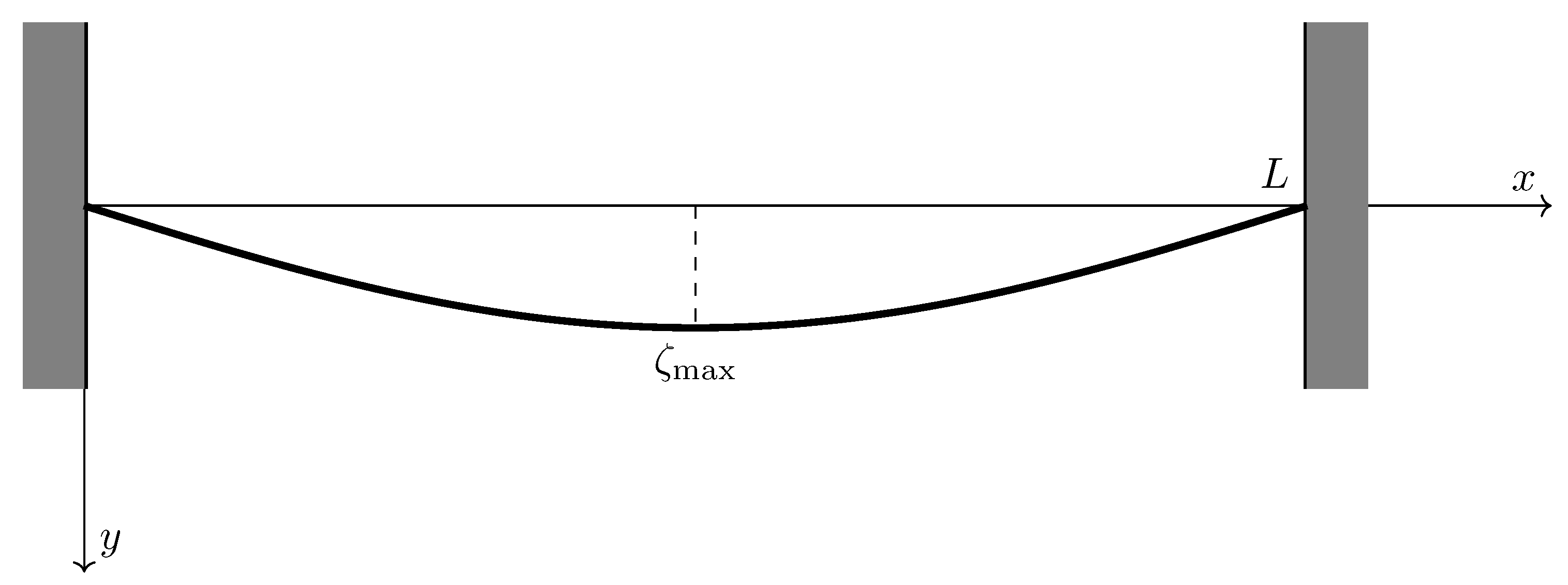
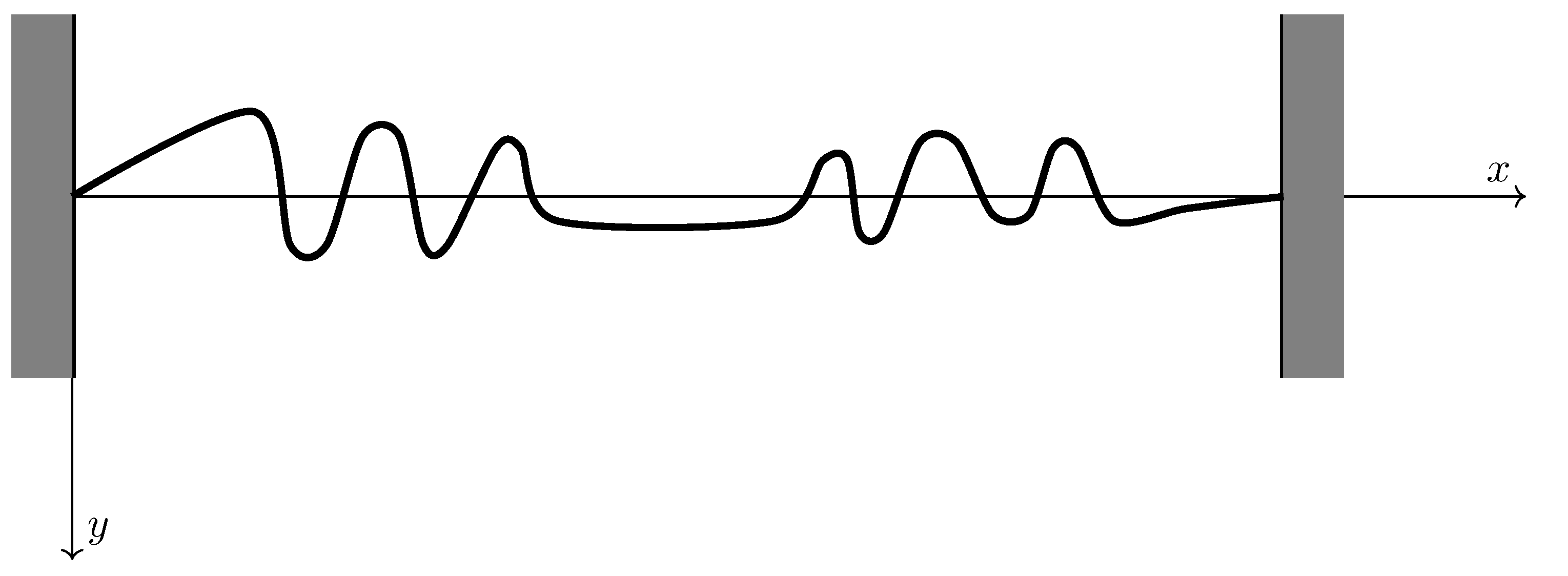
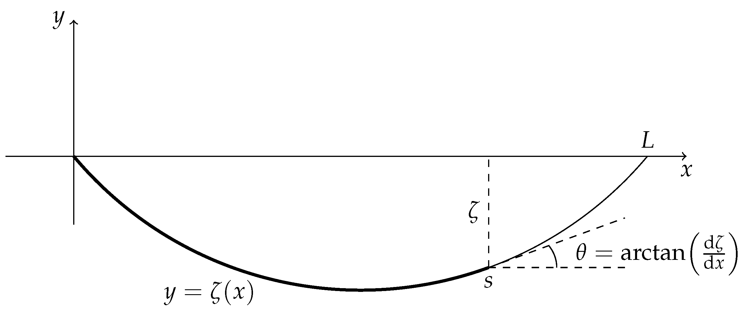
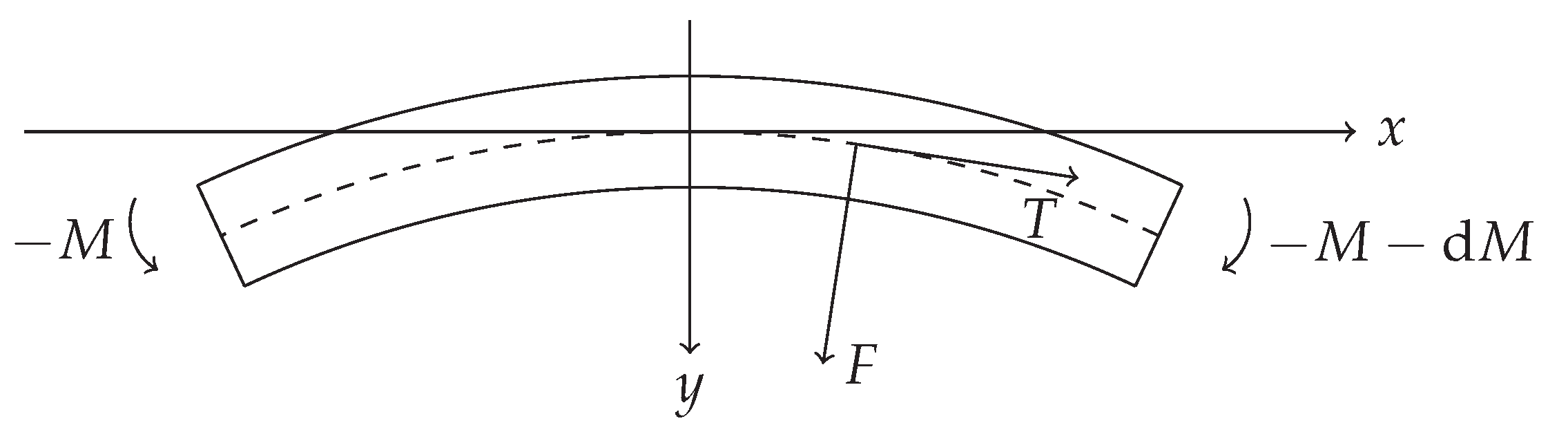
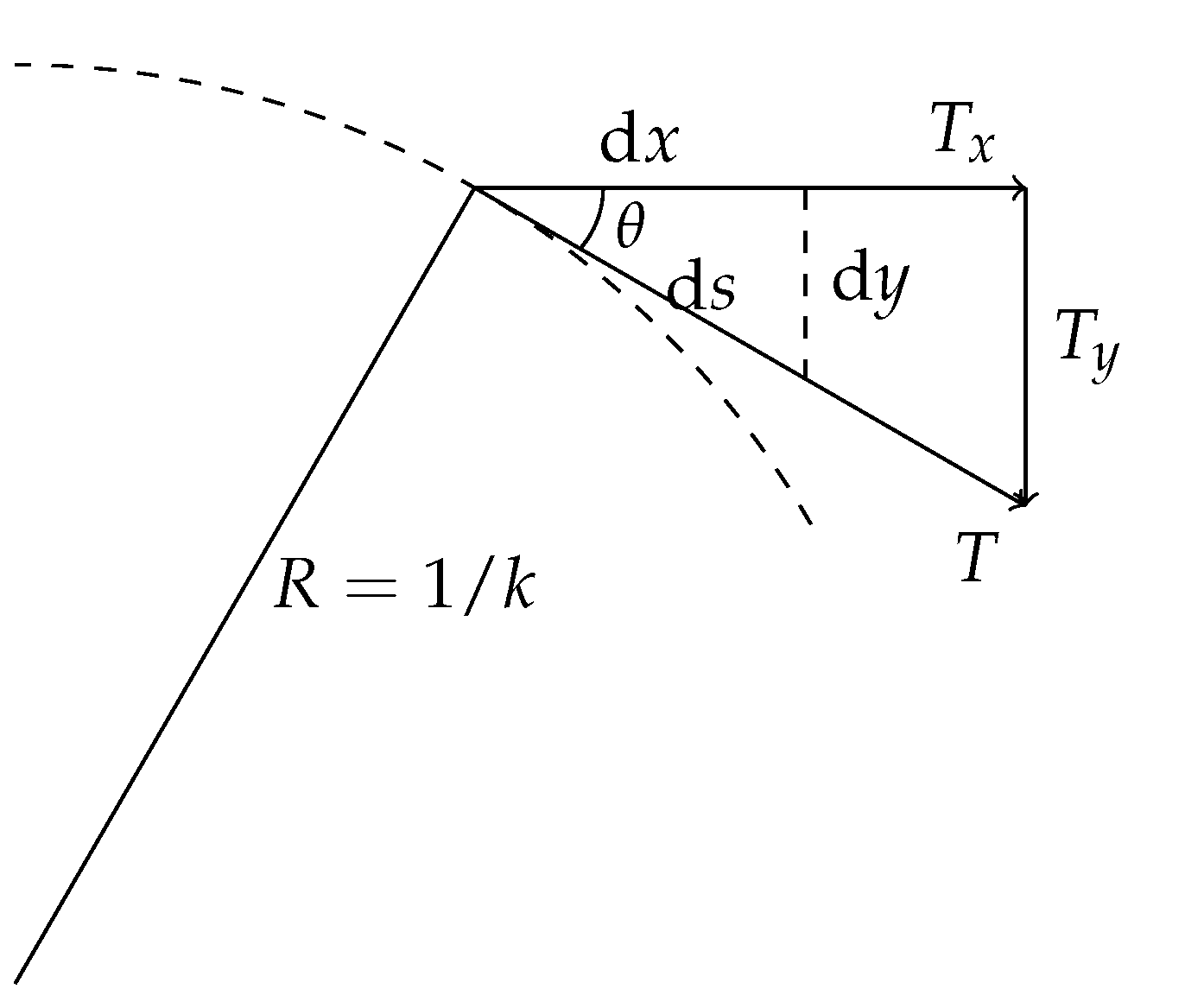
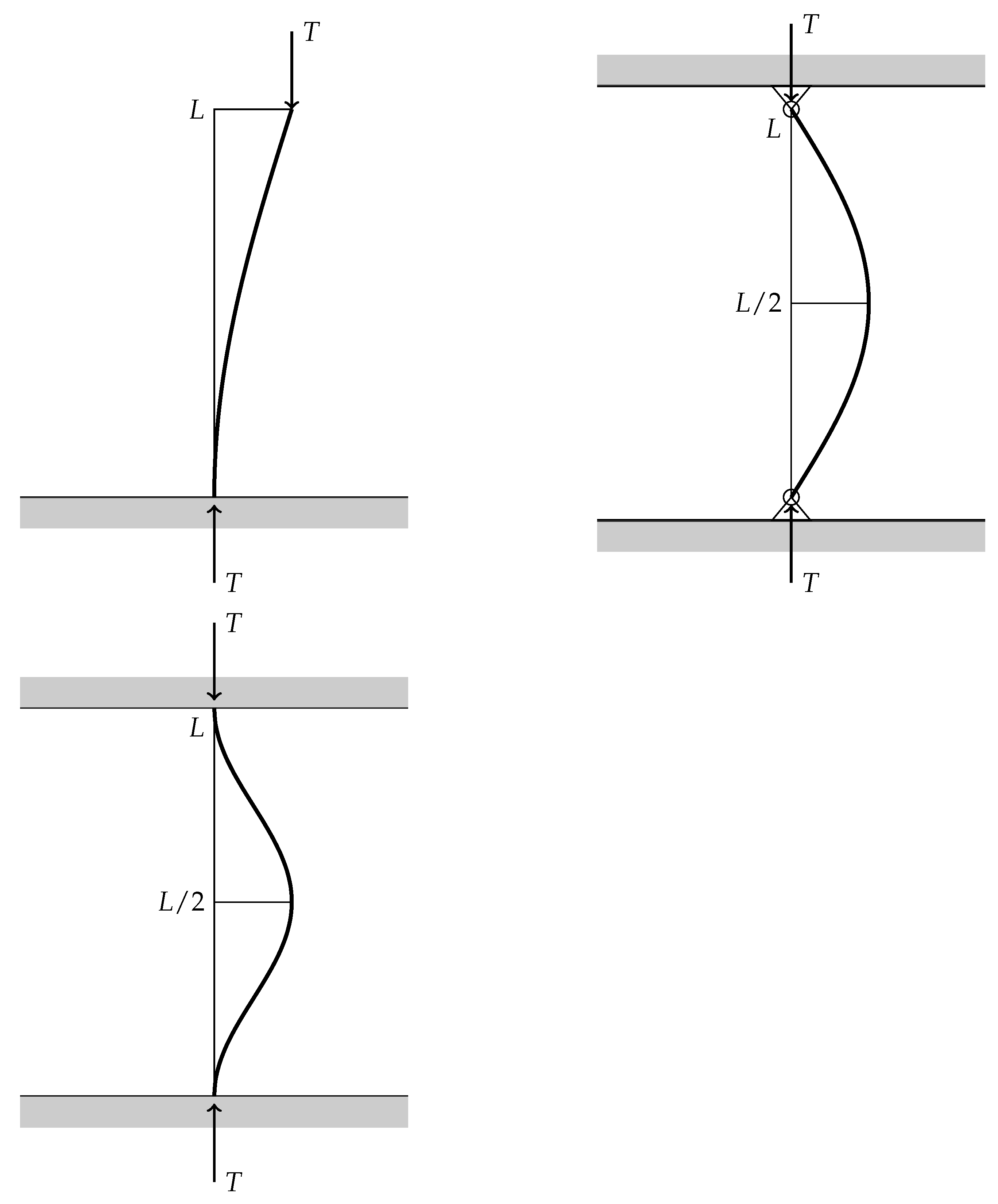
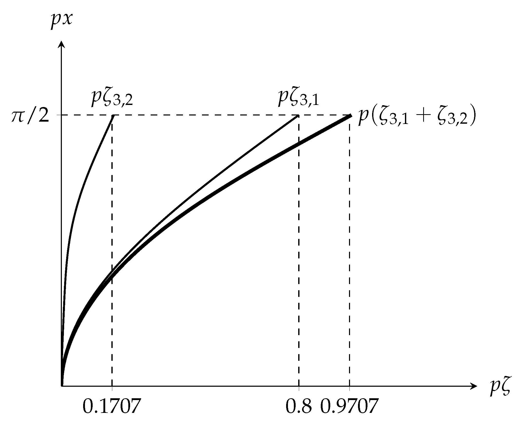
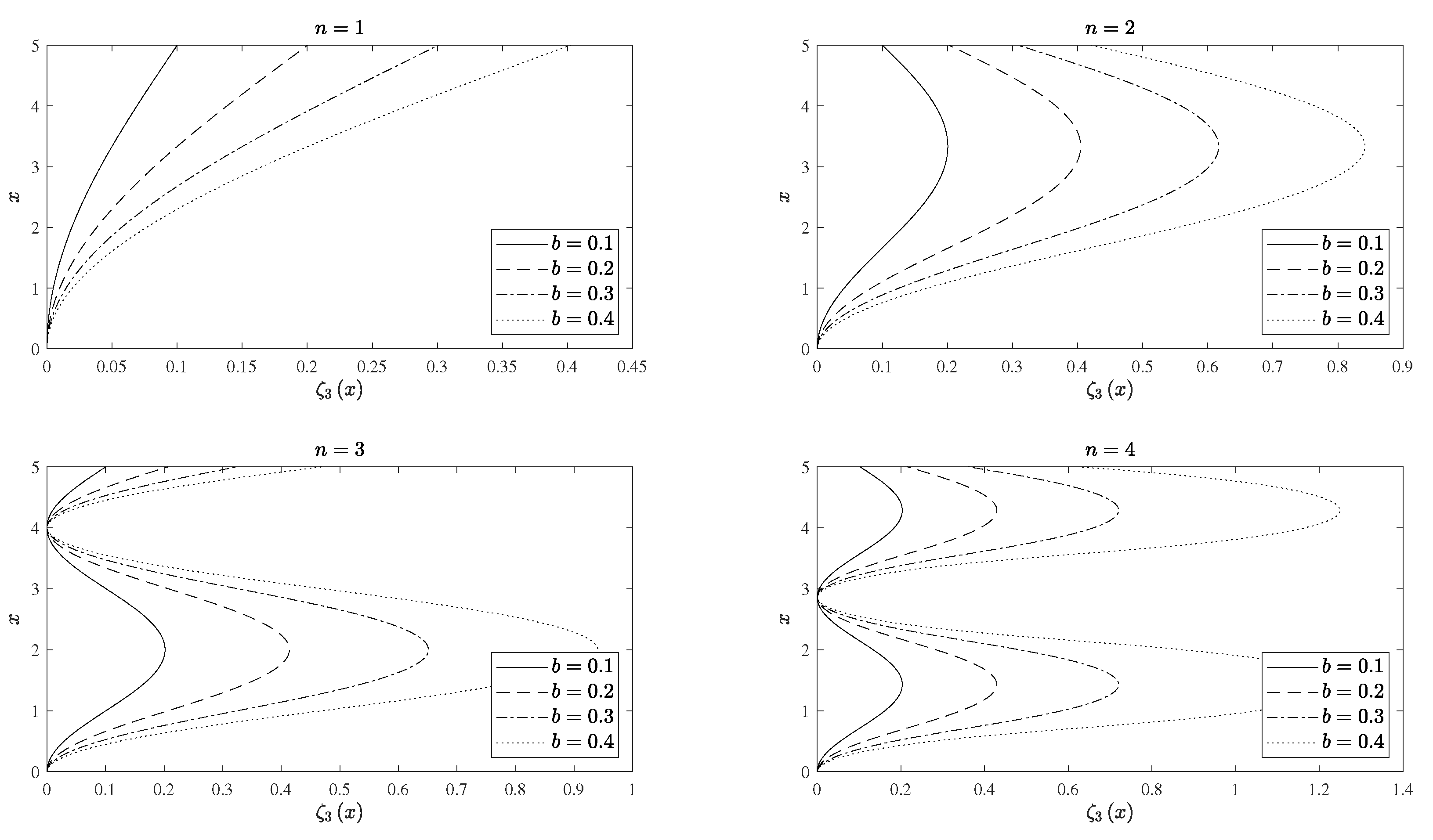
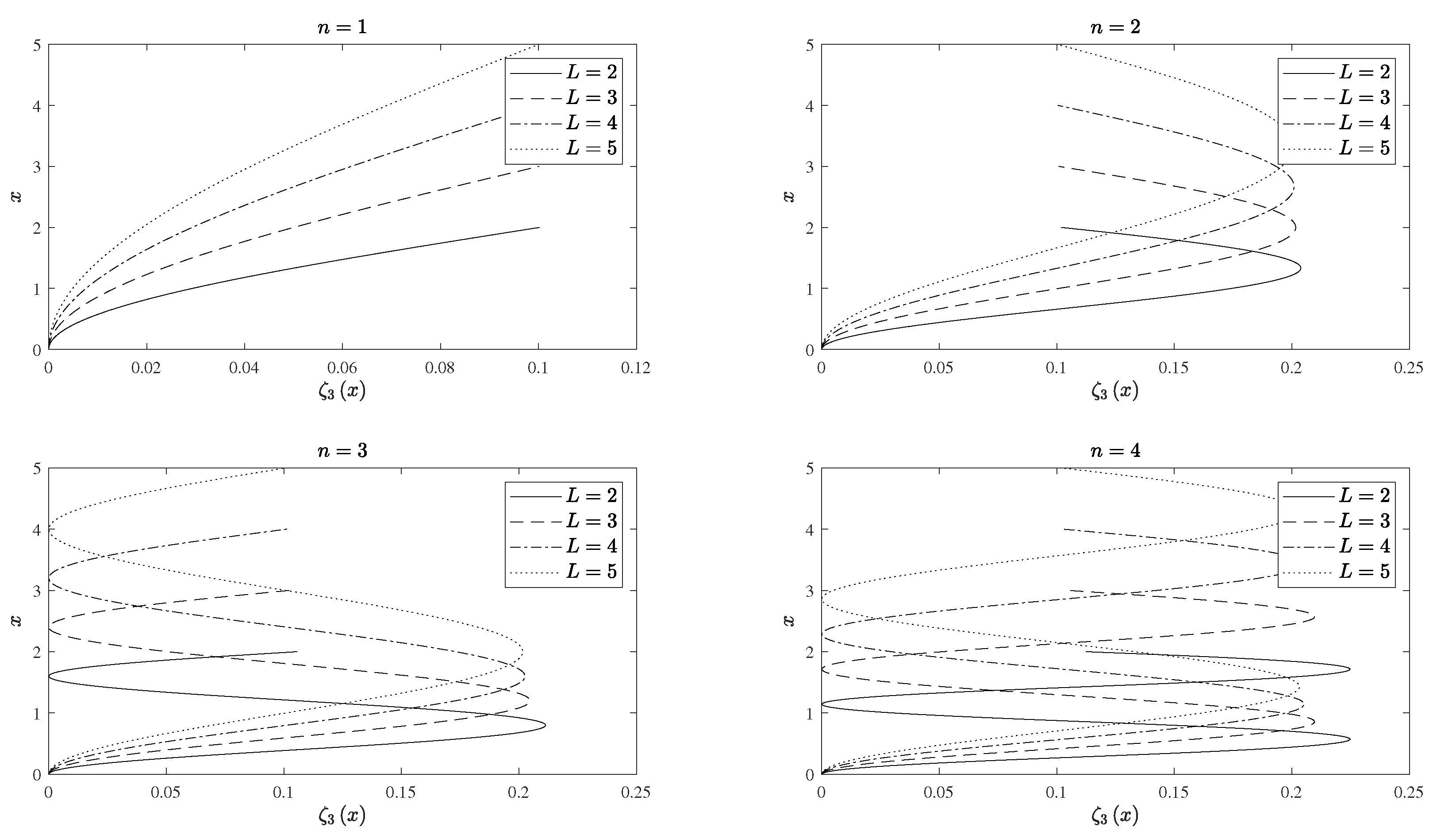
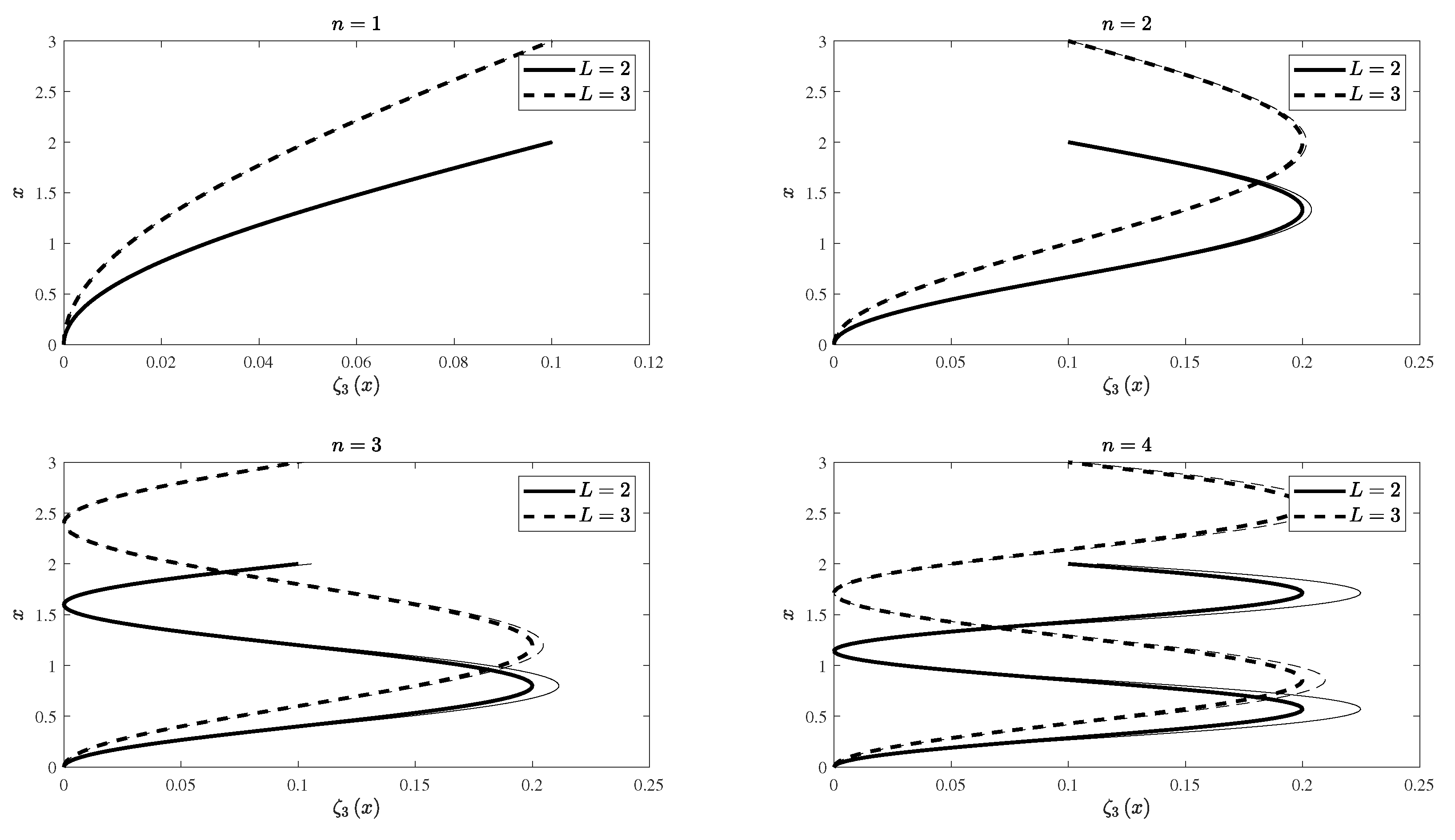
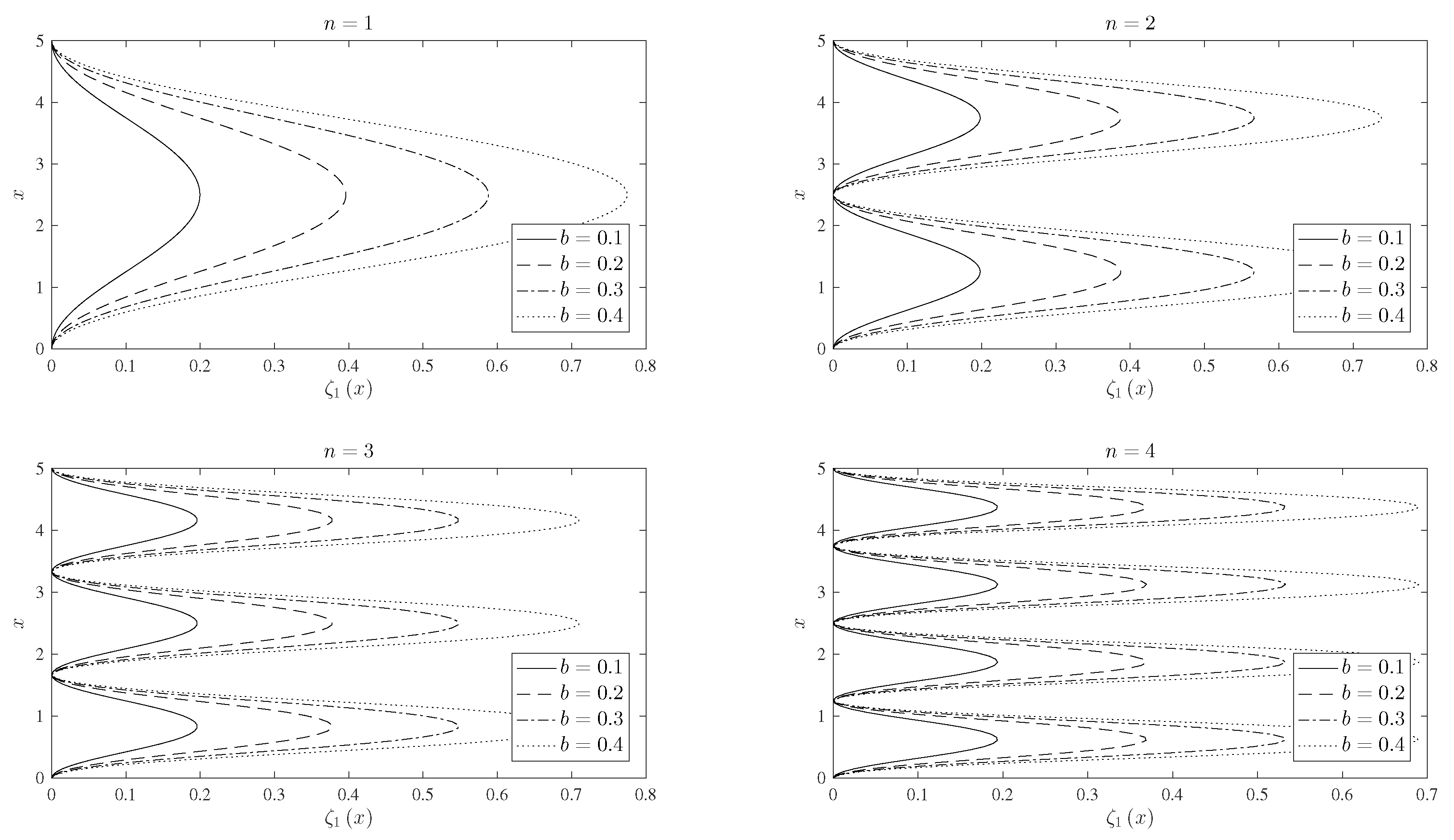
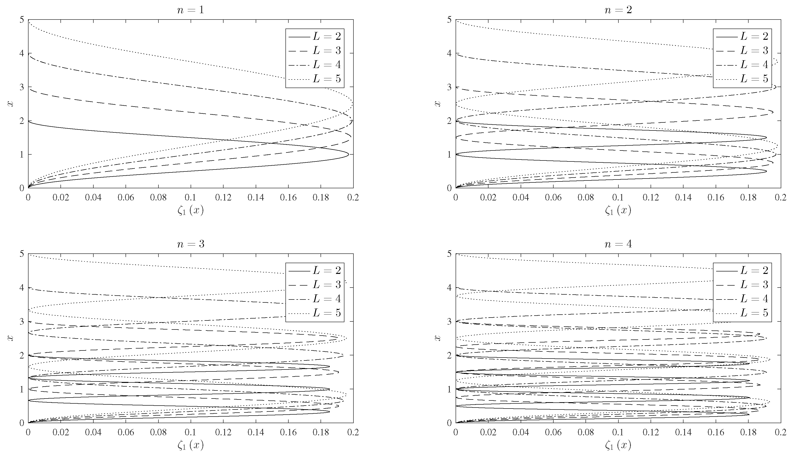
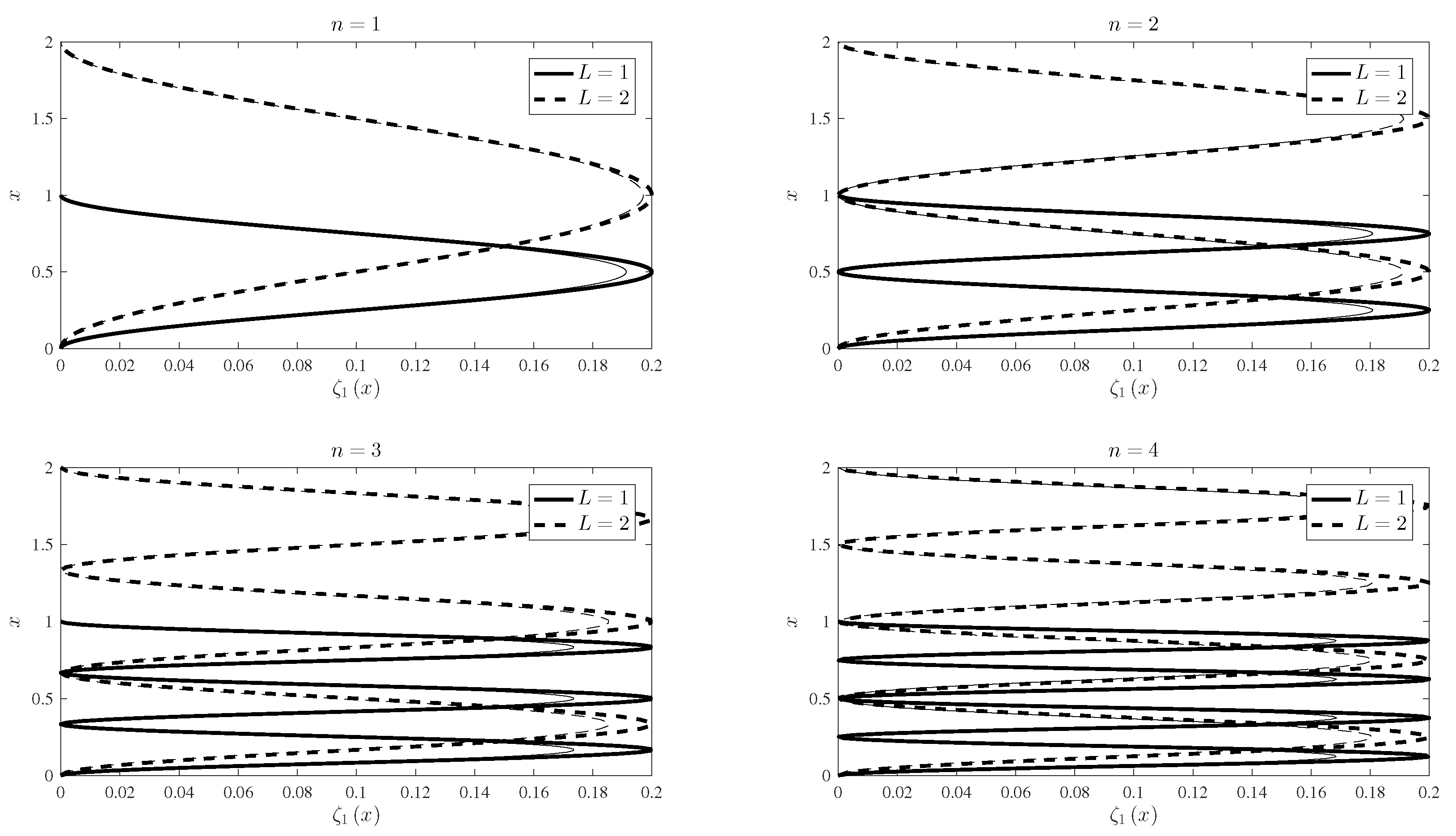
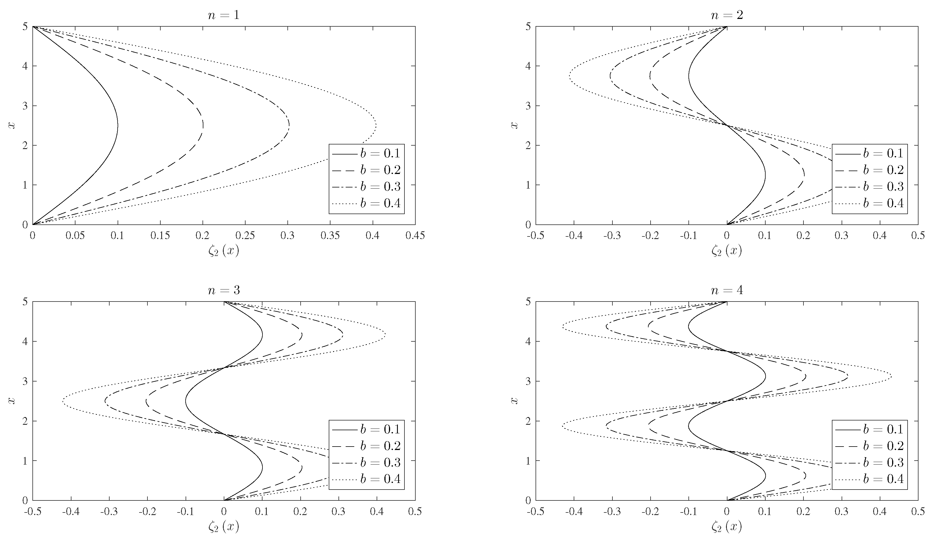
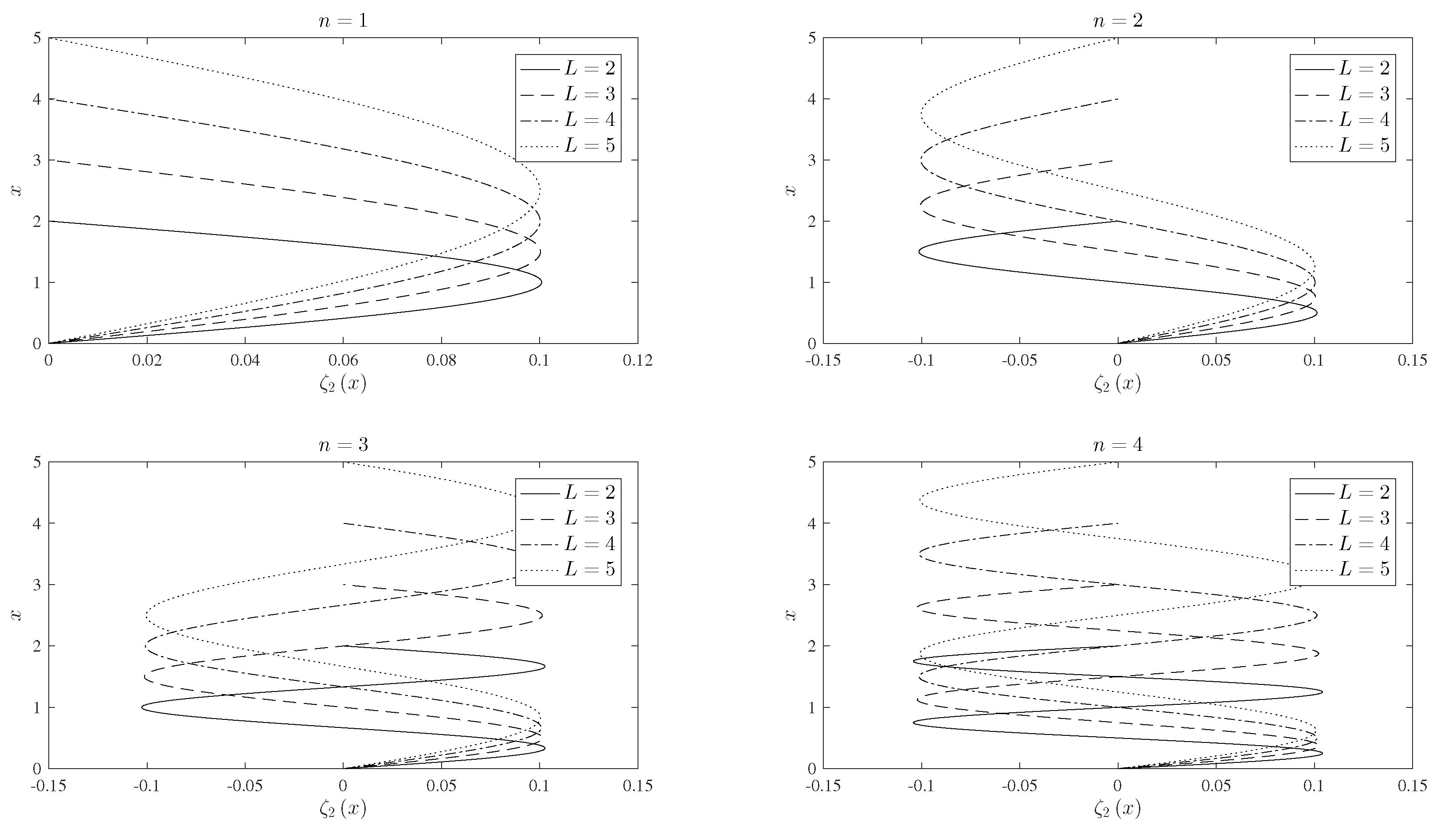
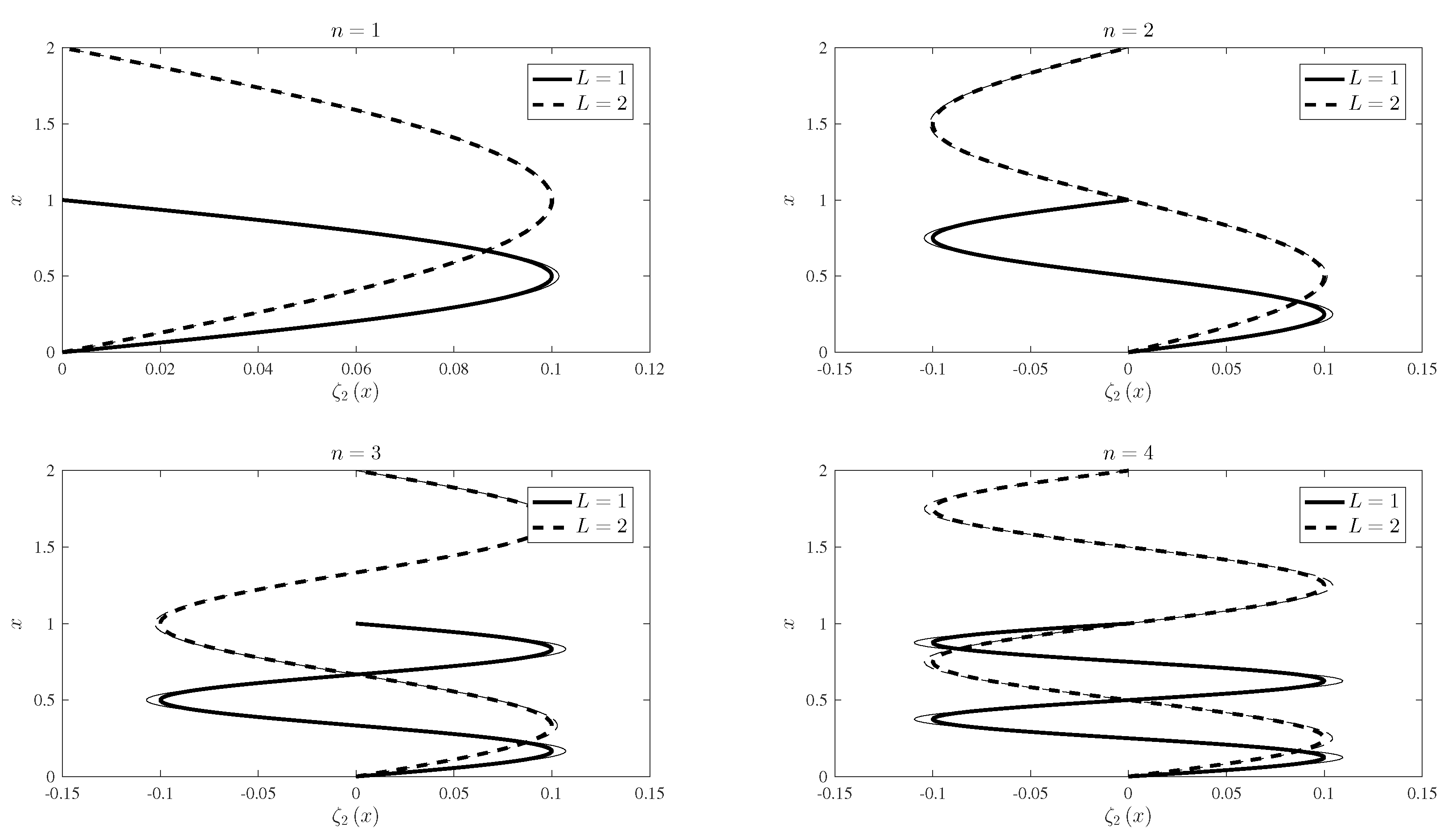
Table 1.
Numerical values for the first seven coefficients of the Equation (44).
Table 1.
Numerical values for the first seven coefficients of the Equation (44).
| Coefficient | |||||||
|---|---|---|---|---|---|---|---|
| Numerical value | 1 |
Table 2.
Number of terms necessary to evaluate the sum in (47a) with absolute and relative errors smaller than , for each length L of the beam and for the first two orders of the buckling load. It also shows the constant G for each case. The parameter b is equal to 0.1.
Table 2.
Number of terms necessary to evaluate the sum in (47a) with absolute and relative errors smaller than , for each length L of the beam and for the first two orders of the buckling load. It also shows the constant G for each case. The parameter b is equal to 0.1.
| Number of Terms | Parameter G | ||||||||
|---|---|---|---|---|---|---|---|---|
| Order | Length | |||||||
| 0.8 | 1 | 2 | 3 | 4 | 5 | 6 | 7 | |
| 1 | 10 | 0.196 | 9 | 0.157 | 7 | 0.079 | 6 | 0.052 | 5 | 0.039 | 5 | 0.031 | 5 | 0.026 | 5 | 0.022 |
| 2 | 30 | 0.589 | 21 | 0.471 | 11 | 0.236 | 9 | 0.157 | 8 | 0.118 | 7 | 0.094 | 7 | 0.079 | 6 | 0.067 |
Table 3.
Successive buckling orders for clamped, pinned and cantilever beams, and comparison of numerical values between the method proposed on this paper and the cited literature [3,4,7].
| Buckling orders | ||||||
|---|---|---|---|---|---|---|
| Beam | Reference | 1st | 2nd | 3rd | 4th | 5th |
| Clamped | Present method | 39.478 | 157.914 | 355.306 | 631.655 | 986.960 |
| Literature [3,4,7] | 39.478 | 157.914 | 355.306 | 631.655 | 986.960 | |
| Pinned | Present method | 9.870 | 39.478 | 88.826 | 157.914 | 246.740 |
| Literature [3,4,7] | 9.870 | 39.478 | 88.826 | 157.914 | 246.740 | |
| Cantilever | Present method | 2.467 | 22.207 | 61.685 | 120.903 | 199.859 |
| Literature [3,4,7] | 2.467 | 22.207 | 61.685 | 120.903 | 199.859 | |
Table 4.
Maximum difference between the linear and lowest-order non-linear approximations of the deformation of the buckled clamped beam for several lengths of the beam and for the first four orders of the buckling load. The parameter b is equal to 0.1. The results are multiplied by 100.
Table 4.
Maximum difference between the linear and lowest-order non-linear approximations of the deformation of the buckled clamped beam for several lengths of the beam and for the first four orders of the buckling load. The parameter b is equal to 0.1. The results are multiplied by 100.
| Order n | Length L | ||||||
|---|---|---|---|---|---|---|---|
| 1 | 2 | 3 | 4 | 5 | 6 | 7 | |
| 1 | 0.866 | 0.288 | 0.137 | 0.079 | 0.051 | 0.036 | 0.027 |
| 2 | 1.909 | 0.866 | 0.469 | 0.288 | 0.193 | 0.137 | 0.102 |
| 3 | 2.612 | 1.423 | 0.861 | 0.563 | 0.392 | 0.286 | 0.217 |
| 4 | 3.131 | 1.909 | 1.252 | 0.866 | 0.626 | 0.469 | 0.363 |
Table 5.
Maximum difference between the linear and lowest-order non-linear approximations of the deformation of the buckled pinned beam for several lengths of the beam and for the first four orders of the buckling load. The parameter b is equal to 0.1. The results are multiplied by 100.
Table 5.
Maximum difference between the linear and lowest-order non-linear approximations of the deformation of the buckled pinned beam for several lengths of the beam and for the first four orders of the buckling load. The parameter b is equal to 0.1. The results are multiplied by 100.
| Order n | Length L | ||||||
|---|---|---|---|---|---|---|---|
| 1 | 2 | 3 | 4 | 5 | 6 | 7 | |
| 1 | 0.144 | 0.040 | 0.018 | 0.010 | 0.007 | 0.005 | 0.003 |
| 2 | 0.433 | 0.144 | 0.069 | 0.040 | 0.026 | 0.018 | 0.013 |
| 3 | 0.0714 | 0.283 | 0.144 | 0.085 | 0.056 | 0.040 | 0.029 |
| 4 | 0.955 | 0.433 | 0.235 | 0.144 | 0.096 | 0.069 | 0.051 |
Table 6.
Maximum difference between the linear and lowest-order non-linear approximations of the deformation of the buckled cantilever beam for several lengths of the beam and for the first four orders of the buckling load. The parameter b is equal to 0.1. The results are multiplied by 100.
Table 6.
Maximum difference between the linear and lowest-order non-linear approximations of the deformation of the buckled cantilever beam for several lengths of the beam and for the first four orders of the buckling load. The parameter b is equal to 0.1. The results are multiplied by 100.
| Order n | Length L | ||||||
|---|---|---|---|---|---|---|---|
| 1 | 2 | 3 | 4 | 5 | 6 | 7 | |
| 0 | 0.083 | 0.021 | 0.009 | 0.005 | 0.003 | 0.002 | 0.002 |
| 1 | 1.716 | 0.383 | 0.167 | 0.093 | 0.059 | 0.041 | 0.030 |
| 2 | 6.975 | 1.135 | 0.477 | 0.263 | 0.167 | 0.085 | 0.079 |
| 3 | - | 2.484 | 0.976 | 0.528 | 0.332 | 0.229 | 0.167 |
Publisher’s Note: MDPI stays neutral with regard to jurisdictional claims in published maps and institutional affiliations. |
© 2021 by the authors. Licensee MDPI, Basel, Switzerland. This article is an open access article distributed under the terms and conditions of the Creative Commons Attribution (CC BY) license (https://creativecommons.org/licenses/by/4.0/).
Share and Cite
MDPI and ACS Style
Campos, L.M.B.C.; Silva, M.J.S. On the Generation of Harmonics by the Non-Linear Buckling of an Elastic Beam. Appl. Mech. 2021, 2, 383-418. https://0-doi-org.brum.beds.ac.uk/10.3390/applmech2020022
AMA Style
Campos LMBC, Silva MJS. On the Generation of Harmonics by the Non-Linear Buckling of an Elastic Beam. Applied Mechanics. 2021; 2(2):383-418. https://0-doi-org.brum.beds.ac.uk/10.3390/applmech2020022
Chicago/Turabian StyleCampos, Luiz M. B. C., and Manuel J. S. Silva. 2021. "On the Generation of Harmonics by the Non-Linear Buckling of an Elastic Beam" Applied Mechanics 2, no. 2: 383-418. https://0-doi-org.brum.beds.ac.uk/10.3390/applmech2020022