Interpretation of Cone Penetration Test Data of an Embankment for Coupled Numerical Modeling


1
WSP-USA, Morristown, NJ 07960, USA
2
School of Engineering and Information Technology, University of New South Wales, Canberra, ACT 2612, Australia
3
Queensland Department of Transport and Main Roads, Brisbane, QLD 4000, Australia
*
Author to whom correspondence should be addressed.
Appl. Mech. 2022, 3(1), 14-45; https://0-doi-org.brum.beds.ac.uk/10.3390/applmech3010002
Submission received: 5 November 2021
/
Revised: 19 December 2021
/
Accepted: 24 December 2021
/
Published: 29 December 2021
(This article belongs to the Special Issue Mechanics Applied in Construction Engineering)
Abstract
:The Nerang Broadbeach Roadway (NBR) embankment in Australia is founded on soft clay deposits. The embankment sections were preloaded and surcharged-preloaded to limit the post-construction deformation and to avoid stability failure. In this paper, we discuss the NBR embankment’s geology, geotechnical properties of the subsurface, and long-term field monitoring data from settlement plates and piezometers. We demonstrate a comparison of cone penetration test (CPT) and piezo cone dissipation test (CPT-u) interpreted geotechnical properties and the NBR embankment’s foundation stratification with laboratory and field measured data. We also developed two elasto-viscoplastic (EVP) models for long-term performance prediction of the NBR embankment. In this regard, we considered both the associated and the non-associated flow rule in the EVP model formulation to assess the flow rule effect of soft clay. We also compared EVP model predictions with the Modified Cam Clay (MCC) model to evaluate the effect of viscous behavior of natural Estuarine clay. Both EVP models require six parameters, and five of them are similar to the MCC model. We used the secondary compression index of clay in the EVP model formulations to include the viscous response of clay. We obtained numerical models’ parameters from laboratory tests and interpretation of CPT and CPTu data. We observed that the EVP models predicted well compared with the MCC model because of the inclusion of soft clay’s viscosity in the EVP models. Moreover, the flow rule effect in the embankment’s performance predictions was noticeable. The non-associated flow rule EVP model predicted the field monitoring settlement and pore pressure better compared to the MCC model and the associated flow EVP model.
1. Introduction
Soft clays are considered problematic soil because of their low bearing capacity, low hydraulic properties, high compressibility, and time-dependent viscoplastic nature [1,2]. When such types of clays experience long-term external loading, the pore water pressure dissipation (PWPD) may be instantaneous, or it may continue for a long time [3]. The PWPD results deform clay and mobilize the shear resistance in response to the external load. However, it is challenging to avoid the construction of geotechnical structures on such types of foundation due to the expansion of urbanization, increase of population, geological values, and associated construction costs. This type of clay may be subject to uneven settlement and lead to partial or even complete failure, which requires subsequent high annual maintenance costs. Construction of geotechnical structures founded on soft clay deposits is considered as one of the geotechnical challenges (see also Indraratna et al. [4]). Therefore, soft clay research is an active field of interest.
In many countries, soft clays are extensively distributed, e.g., in coastal cities in Australia. Roadway embankments close to the coastal precinct in Australia’s Queensland region often traverse soft clay deposits (see Indraratna and Chu [5]). For example, the Nerang Broadbeach Roadway (NBR) embankment was founded on the soft Estuarine clay deposit varying from 5.0 m to 21.0 m (see also Islam et al. [6]). This type of embankment foundation is feeble, and rapid construction is challenging without ground improvement. In the literature, the most common ground improvement methodologies to enhance the engineering properties of clay deposits are preloading, surcharged-preloading, vacuum-preloading, vertical drain, prefabricated vertical drain (PVD), stone column, and chemical stabilization (see also Indraratna et al. [4]; Meena et al. [7]). The application of these technologies depends on many factors, such as subsurface foundation properties, construction cost and time, and the importance of the geotechnical structure. However, the Queensland Department of Transport and Main Roads (QDTMR) found that preloading and surcharged-preloading were the most cost-effective ground improvement methods for the Nerang Broadbeach Roadway (NBR) embankment foundation.
The objective of this paper is to investigate long-term performance of embankments founded on soft clay. When any geotechnical structures are founded on problematic soft clay, as with the NBR embankment, it is essential to predict their long-term performance in order to minimize maintenance cost. In this regard, to address similar challenges, there are numerous numerical models, ranging from elastic models to elasto-viscoplastic models [8,9,10]. In the last few decades, a critical state theory-based elasto-plastic model, such as the Modified Cam Clay (MCC) model [11], has been widely used to predict clay behavior. The MCC model prediction of the coupled hydro-mechanical response of remolded clay has reasonable accuracy. However, from comparison of the observed and the predicted results for the Hall’s Creek test embankment in Canada [12], the Leneghans embankment in Australia [13], the Port of Brisbane in Australia [14], and the Murro test embankment in Finland [15], it is observed that the MCC model has underpredicted the measured responses of soft clays. Therefore, to obtain the realistic behavior of clays, it is important to integrate time-dependent viscosity in the formulation of the constitutive model [16], which is the motivation for the development of elasto-viscoplastic models in this paper.
In the literature, EVP model parameters range from six to forty-four [8,9]. However, to avoid complex mathematical formulations, EVP models have been limited to the associated flow rule in most cases. However, Zienkiewicz et al. [17], among others, reported the importance of the non-associated flow rule model for capturing soft clays’ legitimate behavior. Moreover, for prediction of any real embankment’s performance, there are challenges associated with simplicity of model development and accurate determination of model parameters. Describing the subsurface properties of any problematic soft clay deposit requires special attention. In this regard, along with laboratory tests, the interpretation of field test data, e.g., cone penetration tests (CPT) and piezocone dissipation tests (CPT-u) (see Robertson [18]), may strengthen the delineation of the embankment’s foundation layer. The embankment foundation’s accurate stratification is the primary condition for predicting long-term performances.
We presented a small portion of the Nerang Broadbeach Roadway embankment data in Islam et al. [6]. In this paper, we demonstrate a complete version of the NBR embankment including details of geology, subsurface, and geotechnical properties. We did not present a CPT interpretation of EVP model parameters in Islam et al. [6]. Herein, we discuss details of a CPT interpretation of the NBR embankment’s foundation, and a comparison with laboratory-measured identical values. We also utilise the NBR embankment’s long-term field monitoring data for settlement plates and piezometers. We developed two elasto-viscoplastic (EVP) models to predict the NBR embankment’s observed data. The EVP models’ predictions are compared with the MCC model’s predictions. Details of the EVP models’ formulation, validation, and sensitivity analyses are presented in Islam and Gnanendran [8], Islam et al. [9], and Islam and Gnanendran [10]. We also discussed in our earlier papers the importance of a single surface model and multi-surface model. As we compared the predictions of the EVP and MCC models, we formulated two EVP models considering the MCC equivalent single surface model to evaluate the importance of the viscous behavior of natural clay. In the following sections, we discuss details of the NBR embankment and its finite element simulations.
2. Geology of the Embankment
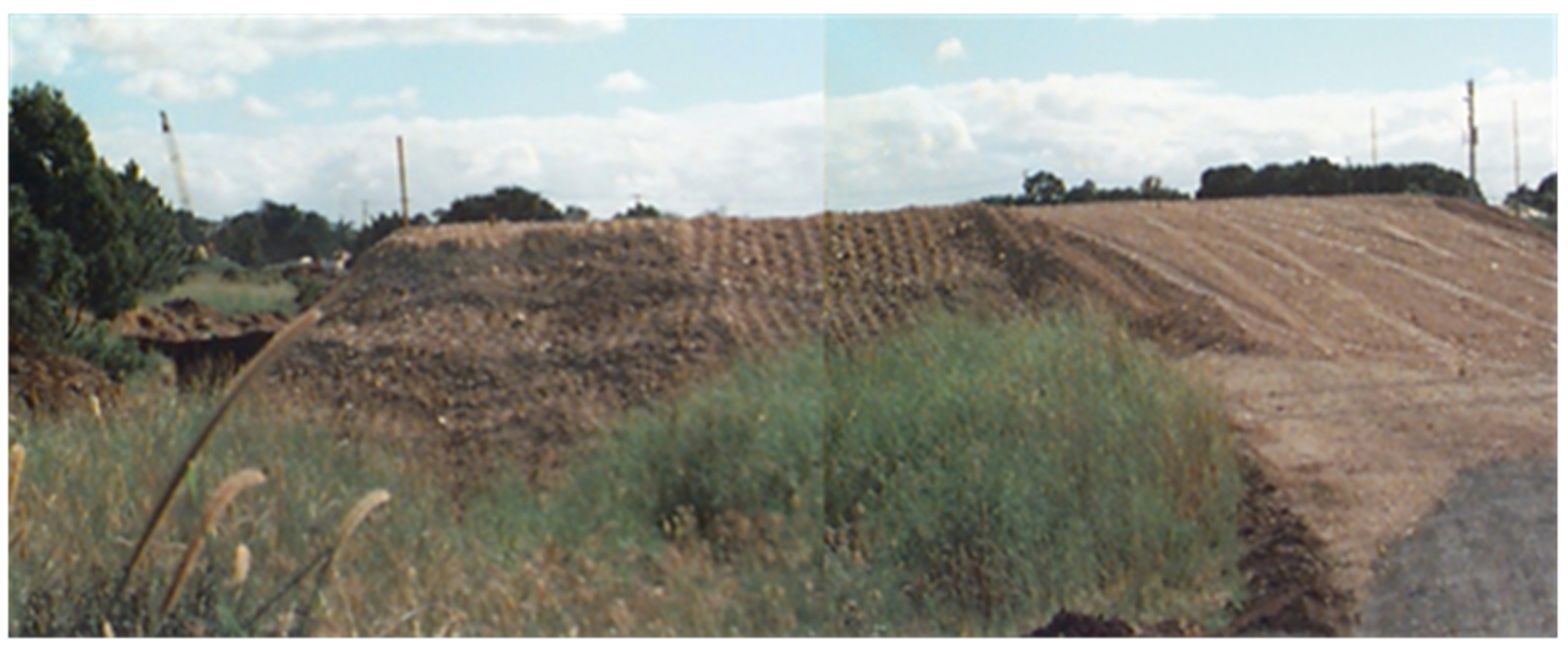
The NBR embankment was constructed in 2001. It is located close to the Gold Coast Highway and the southern part of the Surfers Paradise in Australia’s Queensland region. The NBR embankment’s length and width are 1.30 km and 20.00 m to 28.00 m., respectively. The roadway sections are divided into four zones based on the preloading and surcharged-preloading height. They are Zone 1 (3.50 < H < 4.50), Zone 2 (2.50 < H < 3.50), Zone 3 (1.50 < H < 2.50) and Zone 4 (H < 1.0). However, the QDTMR reported that the first two sections were problematic (Main Roads [19]; Main Roads [20]; Main Roads [21]; Main Roads [22]) due to (i) the compressible soft clay layer, (ii) the presence of the organic component, (iii) the stability problem, and (iv) ongoing time-dependent settlement due to the viscous nature of the clay deposit. Therefore, the QDTMR installed a total of 18 settlement plates and three piezometers to monitor the long term responses of the embankment foundations. The QDTMR did not install inclinometer or other instrumentation for the NBR embankment. We present the embankment construction area in Figure 1.
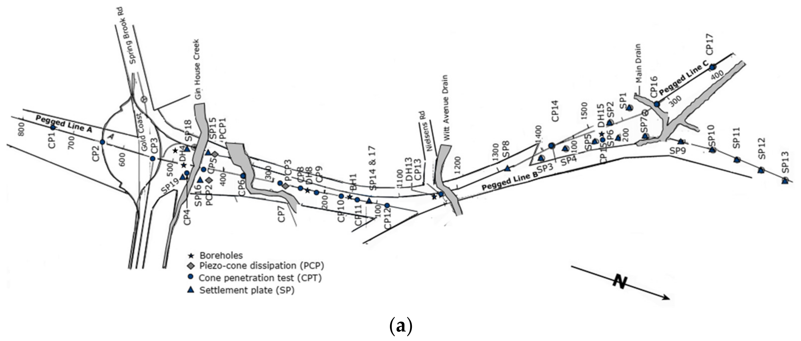
The site plan and the investigation locations and monitoring points are presented in Figure 2a. The NBR embankment’s longitudinal section is demonstrated in Figure 2b. It is worth noting that close to the Gin House Creek (see Figure 2), clay deposits involve a soft compressible clay layer with 8.4% organic contents. In the following sections, we discuss the geology of the NBR embankment.
The NBR embankment’s geology consists of soft sensitive clay overlaying the greywacke and the argillite bedrock. The clay is the Cainozoic Estuarine alluvial type with a thickness of 5.00 to 21.00 m. The NBR embankment’s foundation is divided into three distinct layers. They are the upper alluvium, the lower alluvium, and the bedrock (Figure 2b). Details are presented below.
The upper alluvium developed mainly due to the flood plain deposit generated from the existing drainage systems. It reflects the Estuarine and the dunal depositional history, and consists of a mixture of silt, sand, and clay. The layer composition is not uniform. The upper alluvium layer’s depth varies from 2.00 m to 6.00 m.
The lower alluvium was intercepted in boreholes between the upper alluvium and the bedrock (see Figure 2b). The thickness of this layer varies between 2.0 m to 20.0 m. The mangrove mud developed the alluvium layer. This layer consists of the older alluvium, including over consolidated mangrove muds, river channels, and flood plain deposits. River channels have been cut close to this deposit. From borehole reports and cone penetration test data, the lower alluvium is divided into three sub-divisions depending on physical properties. They are silty clay-1, silty clay-2, and silty clay-3. The lower alluvium is highly compressible and considered soft to stiff clay.
The bedrock is the lowest level, which consists of the greywacke and the argillite bedrock of the Neranleigh–Fernvale beds.
3. Subsurface Profile of the Embankment
The QDTMR carried out two subsoil investigations to explore the NBR embank-ment’s geotechnical properties in 1991 and 1999 (see Main Roads [20,21]). These reports indicated poor foundation conditions. Therefore, from 2000 to 2001, the QDTMR performed additional investigations (Main Roads [22,23]). These inspections include six boreholes, twenty electric cone penetrometer tests (CPT), four piezocone dissipation tests (CPT-u), field vane shear tests, and pocket penetrometer tests. Details of investigation locations are also illustrated in Figure 2a. In the following sections, we present the subsurface profile of the NBR embankment.
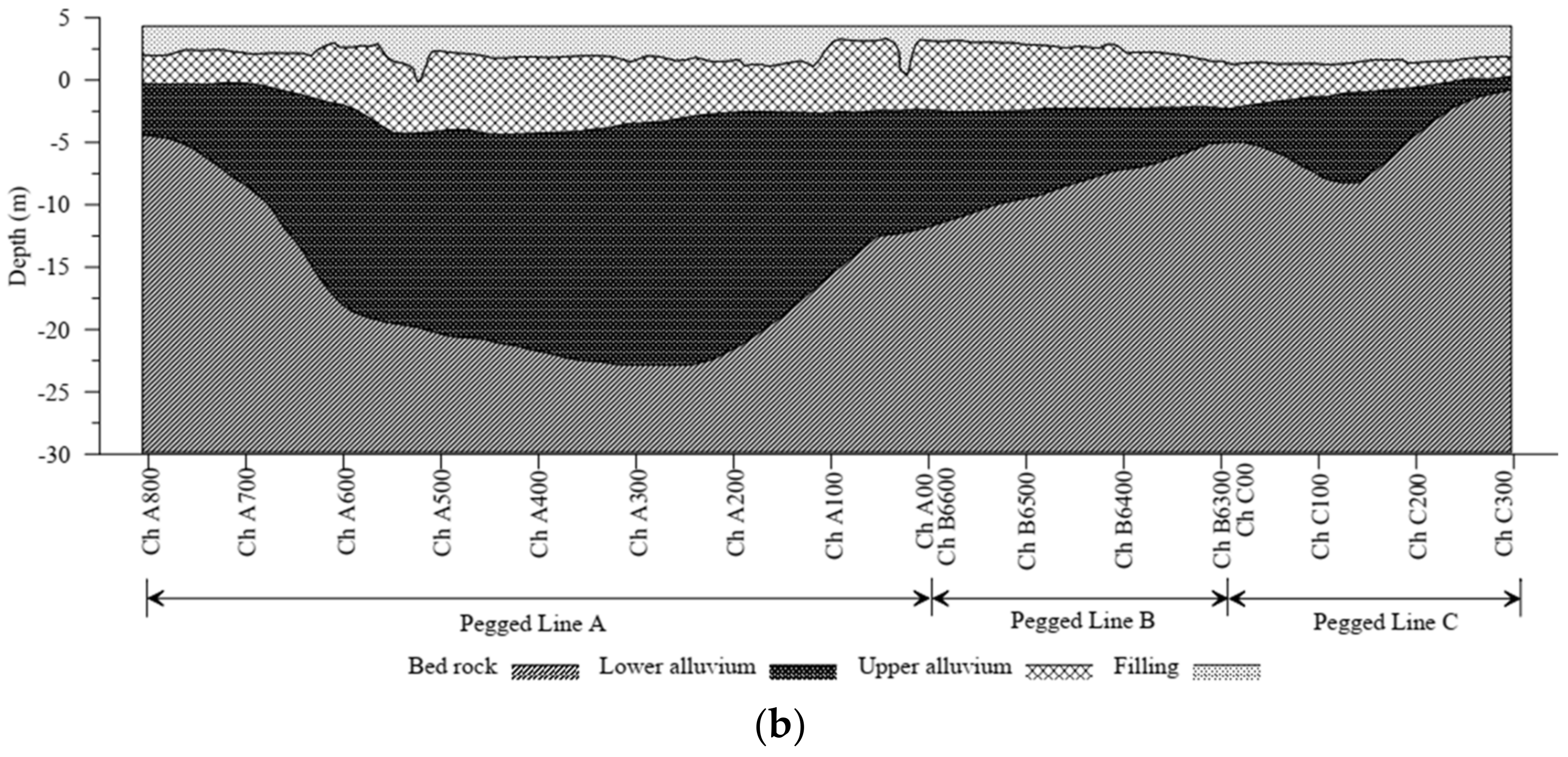
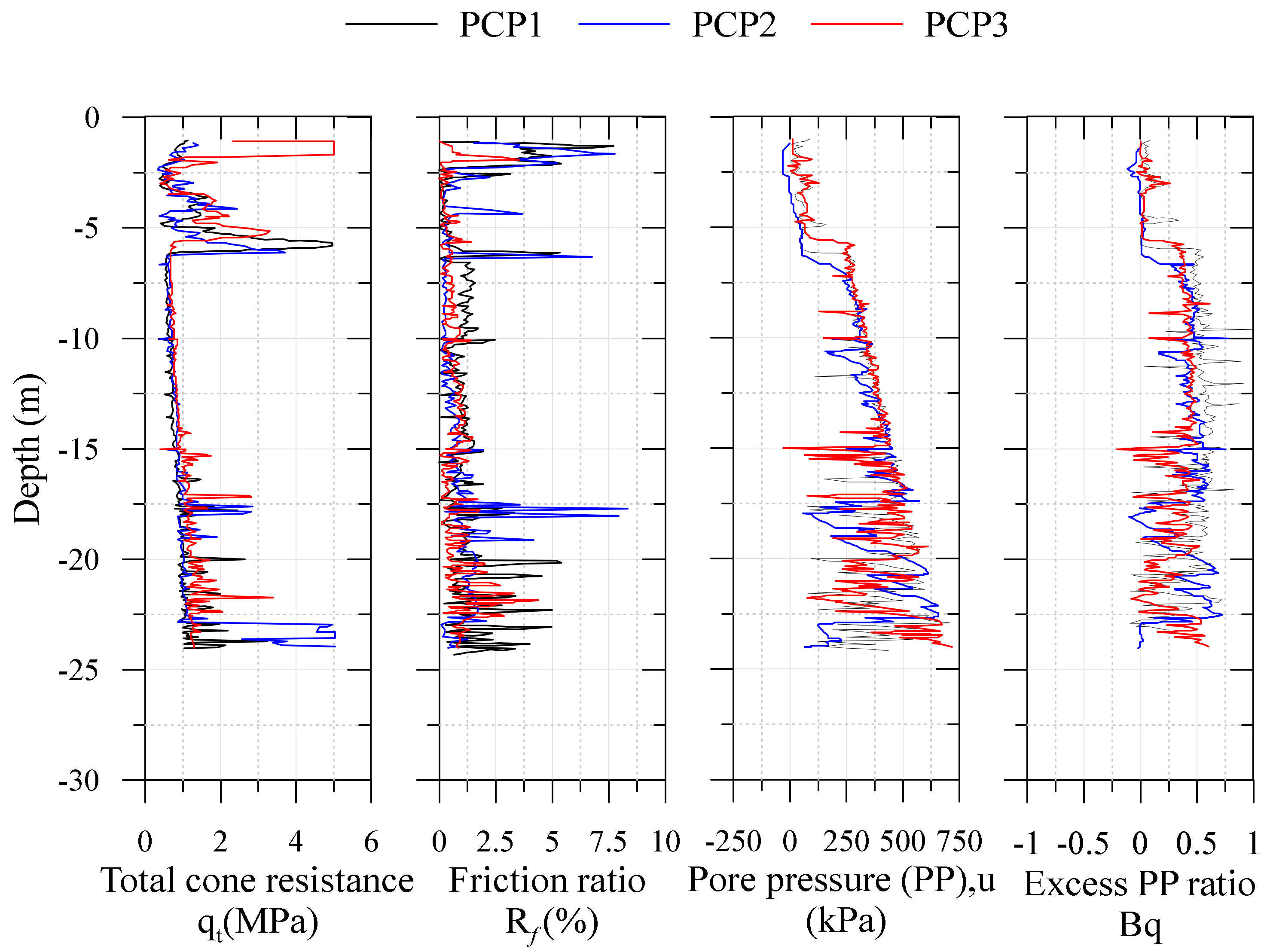
Along the NBR embankment length, the Gin House Creek (see Figure 2) is the most problematic zone, and is also the point of interest in this paper. The observed monitoring data of the Gin House Creek area and the finite element simulations are compared herein. CPT and CPT-u tests data close to the Creek location of the embankment are presented in Figure 3. The subsurface stratification of the embankment was performed using boreholes data, laboratory tests, CPT, and CPT-u data.
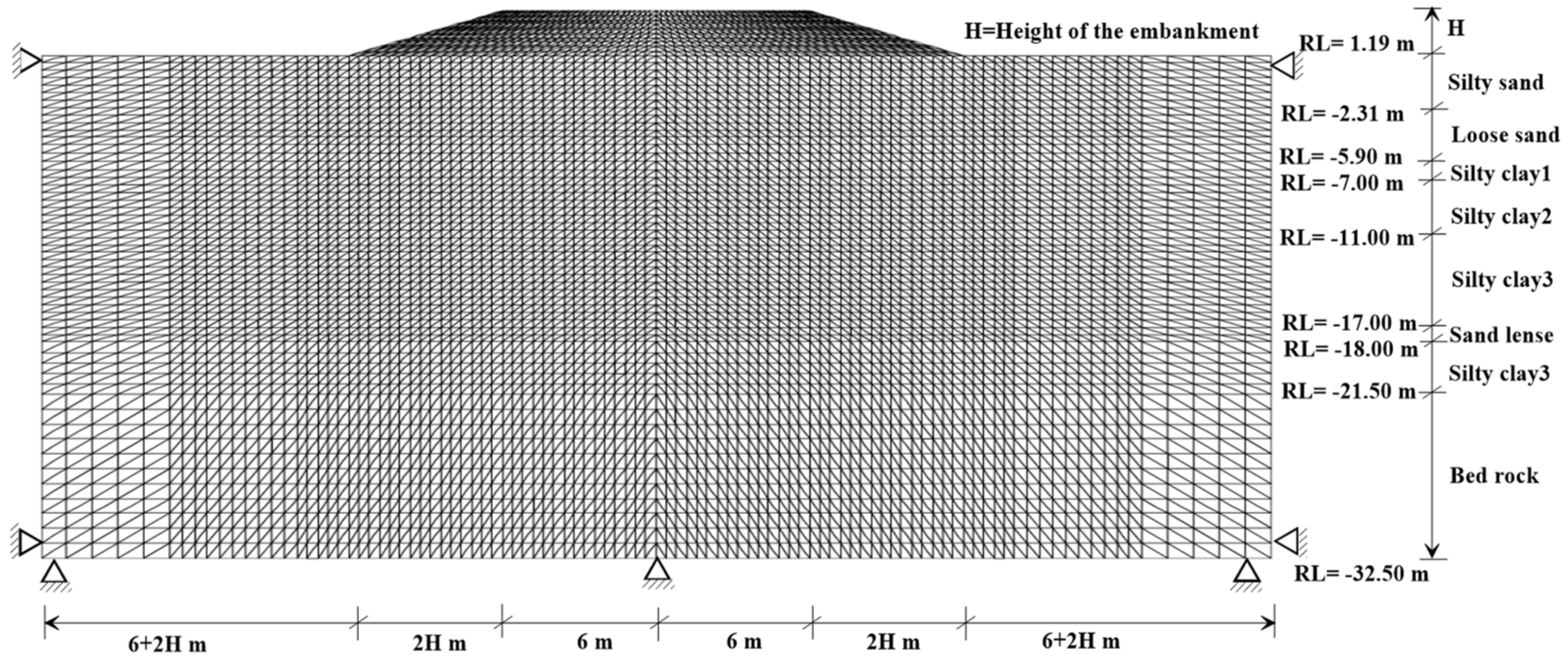
From boreholes and CPT data, it was observed that in the Reduced Level (RL) 1.19 m to −2.00 m, the soil deposit was dark grey, lightly moist, loose silty sand. In this layer, the organic root fragments were also noticed. Then, at RL = −2.00 m to −5.90 m, the soil was grey, wet, very loose to loose sand. From the vane shear test report, a similar soil type was found at this depth. Robertson and Cabal [23] and Mayne [24] reported that during the CPT test in sandy layers, negative pore pressure developed due to the dilation of granular materials. Identical negative pore pressure responses were observed in CPT data at RL = −3.50 m (see Figure 3). At RL = −5.90 m to −7.00 m, soft grey moist clay with shells representing a silty clay-1 layer was noticed. At RL = −7.00 m to −11.00 m, there was a silty clay-2 layer that was dark grey, moist, and soft to firm silty clay with traces of shells and shell fragments. A silty clay-3 was observed at RL = −11.00 m to −21.50 m, where the Estuarine mud was brownish grey, moist, and stiff to very stiff. A thin sand lens was observed from CPT test data at RL = −17.00 m to −18.00 m (see Figure 3). After RL = −21.50 m, a dense silty clay to dense sand layer was noticed.
In general, the permeability of sand is high, while in clay, permeability is low (see Mayne [24]). Therefore, the pore pressure developed in the sandy layer is small compared to the clay layer. The cone tip resistance increases in the sand layer, but the frictional resistance decreases (see also Mayne [24]; Robertson and Cabal [23]). The pore pressure and the hydrostatic pressure ratio for sandy soil is less than or equal to 1.0. The ratio for soft clay is about 3.0, and increases with the increase of the clay layer’s stiffness. Similar trends for sand and clay layers were observed in RL = 1.19 m to –5.90 m and RL = −5.90 m to −21.50 m, respectively (see Figure 3).
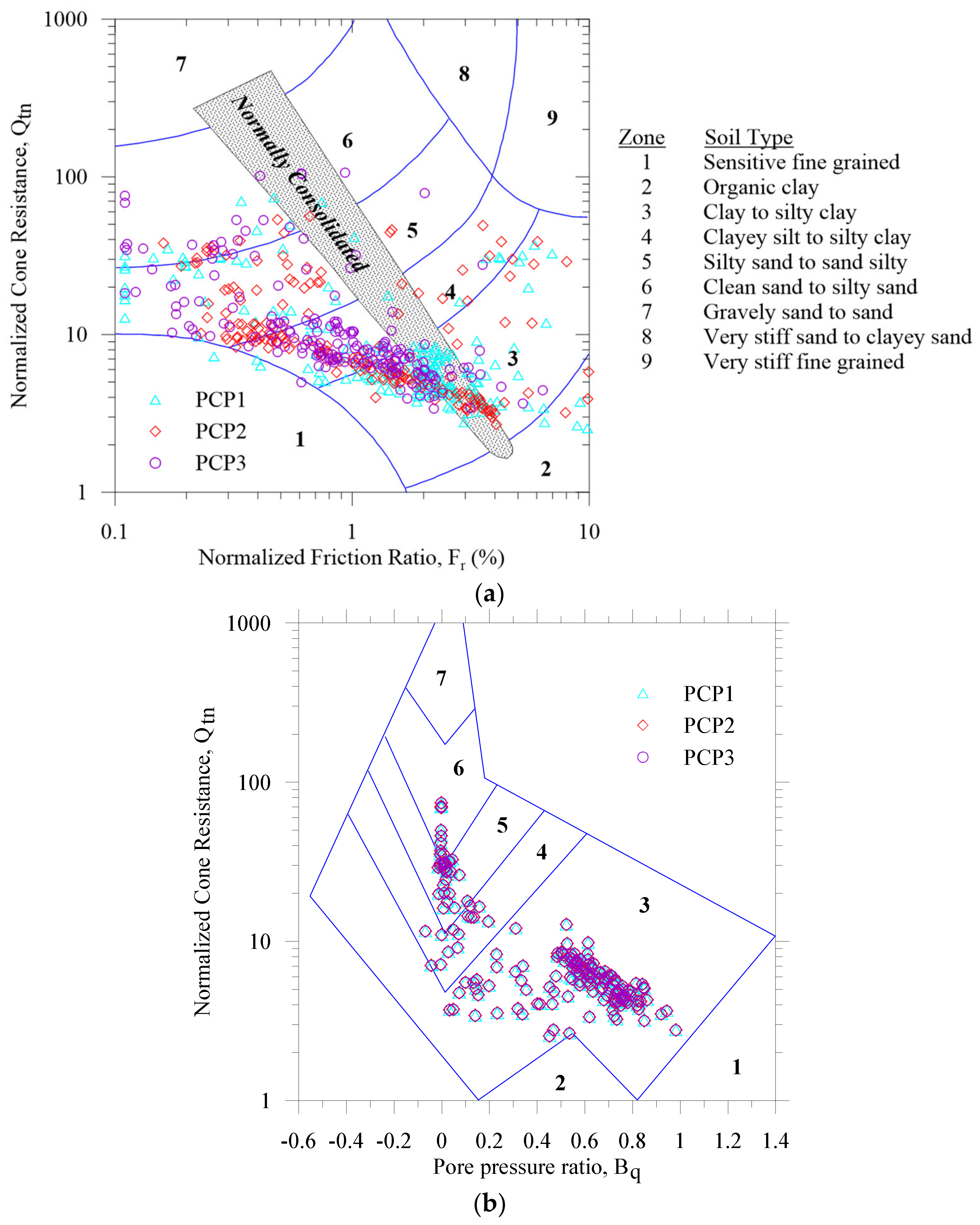
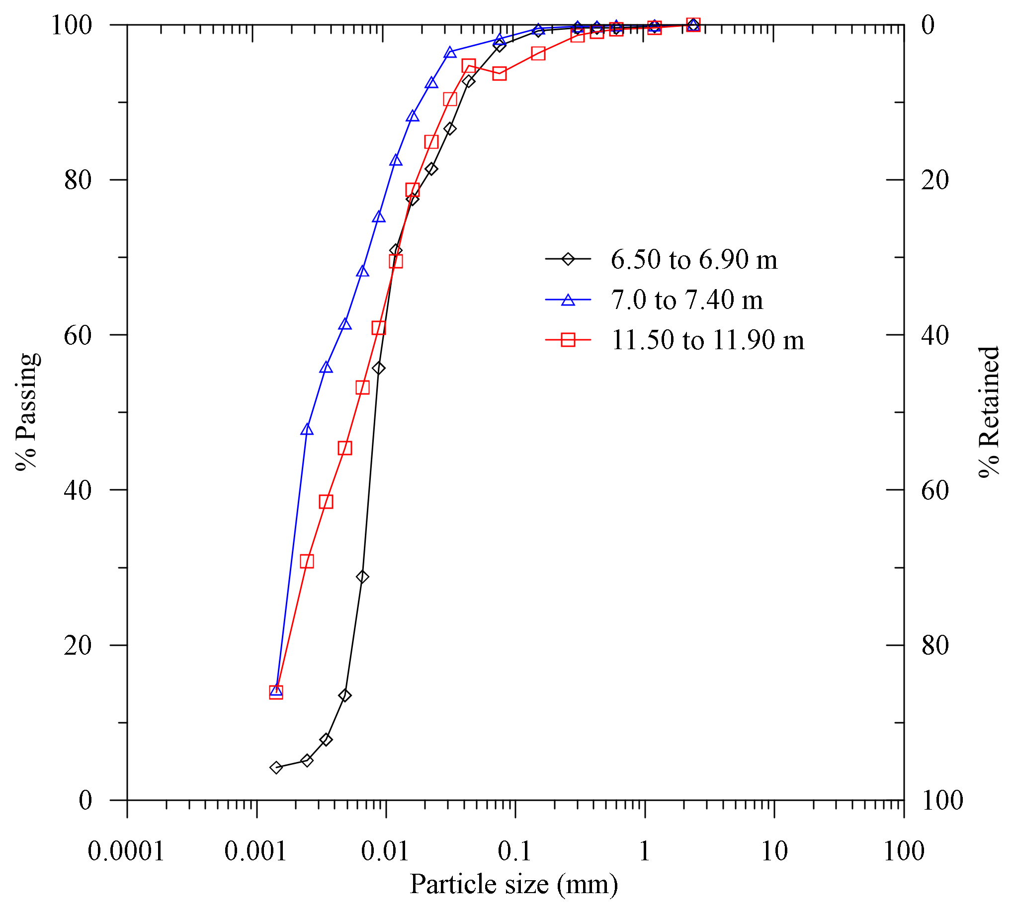
We illustrate Robertson’s [25] proposed CPT-based soil classification in Figure 4. It was observed that in most cases, the NBR embankment’s foundation soils fall in Zones 3 to 6, representing clay, silty clay, silty sand, and sand. Soils in Zones 1 and 2 (see Figure 4), demonstrate sensitive fine grained to organic clay. Laboratory tests also showed 8.35% organic content at 10.0 m to 10.4 m depth. The particle size distribution (PSD) of the undisturbed samples is presented in Figure 5. The experimentally observed PSD and the organic content test also support the CPT interpretation of the NBR embankment foundation’s clay.
4. Geotechnical Properties
A series of 50.00 mm undisturbed samples were collected from different depths of the NBR embankment’s foundation. Then, laboratory tests were performed to discover the NBR embankment foundation’s geotechnical properties. Moreover, we interpret CPT and CPT-u test data to delineate the NBR embankment foundation and compare it with boreholes data and laboratory tests to justify the foundation stratification. In the following sections, we discuss the geotechnical properties of the Gin House Creek area. Moreover, we consider similar embankment sections for coupled finite element simulations (see Section 5).
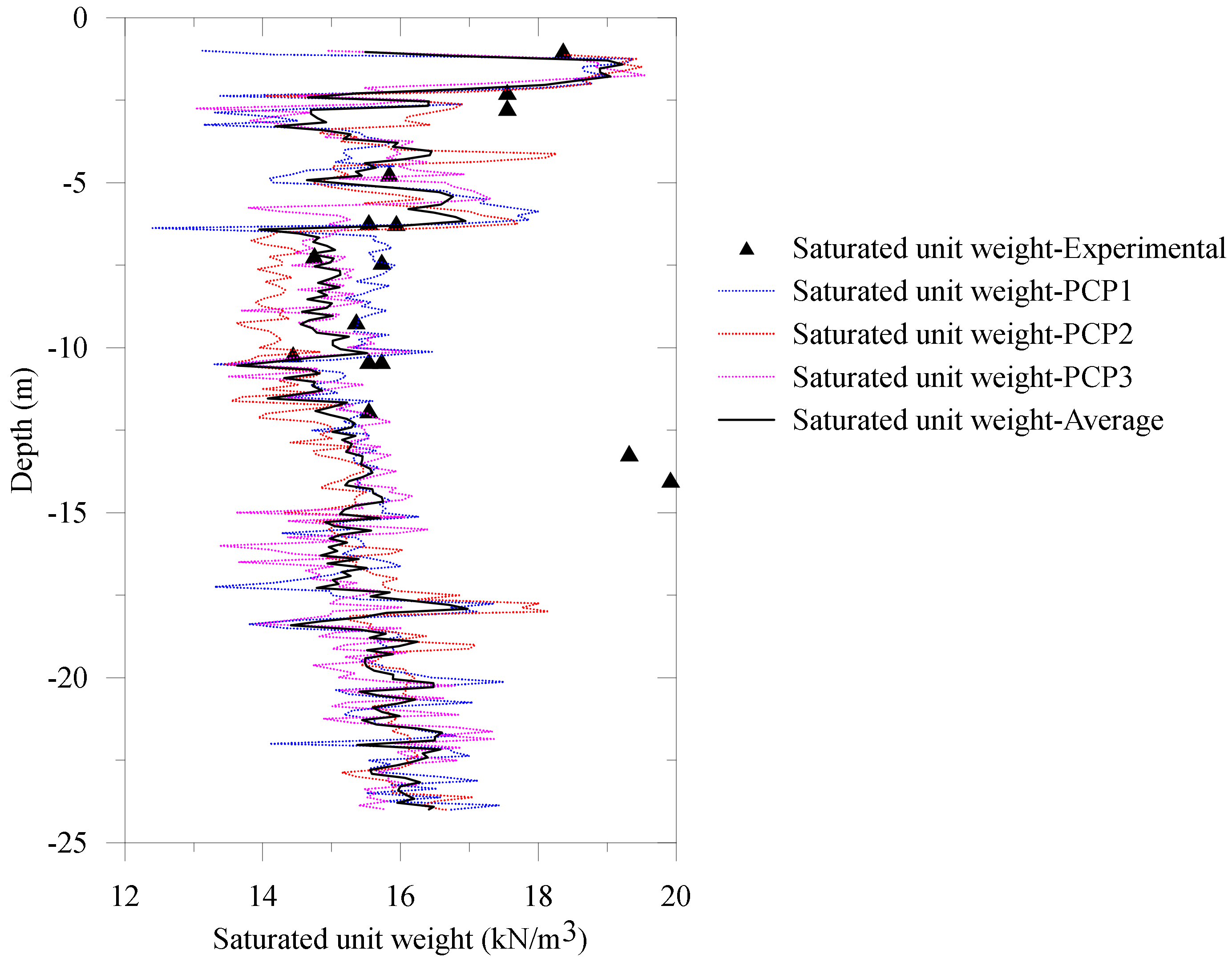
The NBR embankment foundation layer at the chainage 400 to 500 (see Figure 2a), comprised a silty sand layer, loose sand, silty clay-1, silty clay-2, sand lense, and silty clay-3. The saturated unit weight obtained from the laboratory experiments in these locations ranged from 14.44 kN/m3 and 19.92 kN/m3, as is illustrated in Figure 6.
CPT interpreted saturated unit weight is presented as (see Mayne [24])
where z is the soil layer depth, while is the shear wave velocity (m/s). in kN/m3
For the NBR embankment foundation layer, it is observed that Hegazy and Mayne’s [26] proposed illustrated well the experimentally obtained (see Equation (1)) and is given by
Here in m/s, while and are the corrected cone resistance and the cone resistance, respectively. is the measured pore pressure behind the cone, and a is the net area ratio, which ranged between 0.70 and 0.85 (see also Mayne [24]). In addition, is the sleeve friction. Following Robertson and Cabal [23], the unit weight is written as
where , is the unit weight of water, is the atmospheric pressure, and is the friction ratio.
A comparison of the laboratory measured saturated unit weight and the CPT interpreted values is presented in Figure 6. An average saturated unit weight is calculated from three sets of CPT data (see Figure 3). It is observed that laboratory measured fitted best with the CPT interpreted average (see Figure 6). However, a deviation of two data points was observed at 13.2 m and 14.0 m depth, which are located at BH1 (see Figure 2a).
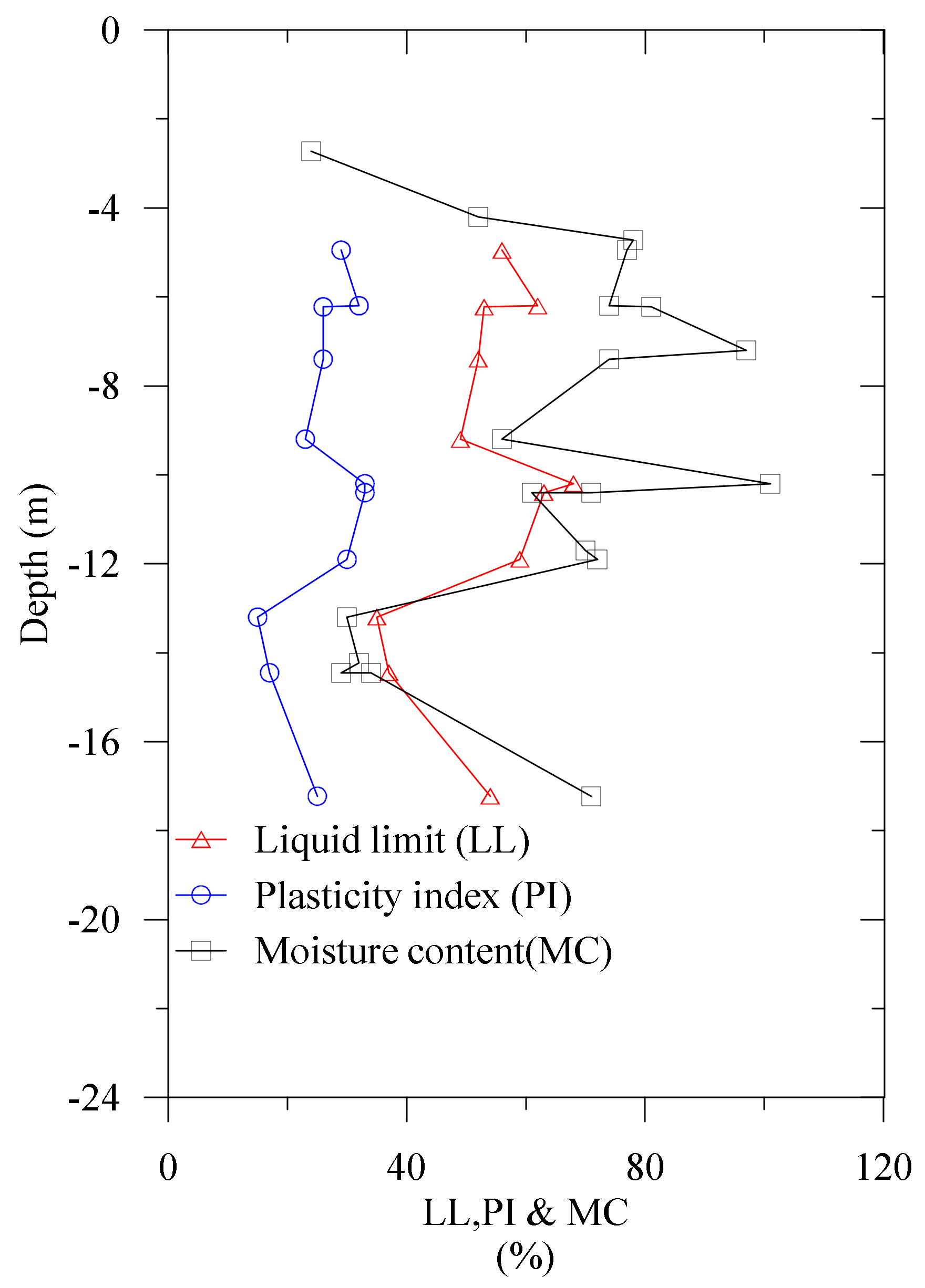
The moisture content (24.0 to 101.0%), the plasticity index (15.0 to 33.0), and the liquid limit (35.0 to 68.0) of the NBR embankment’s foundation were obtained from the laboratory tests which are illustrated in Figure 7.
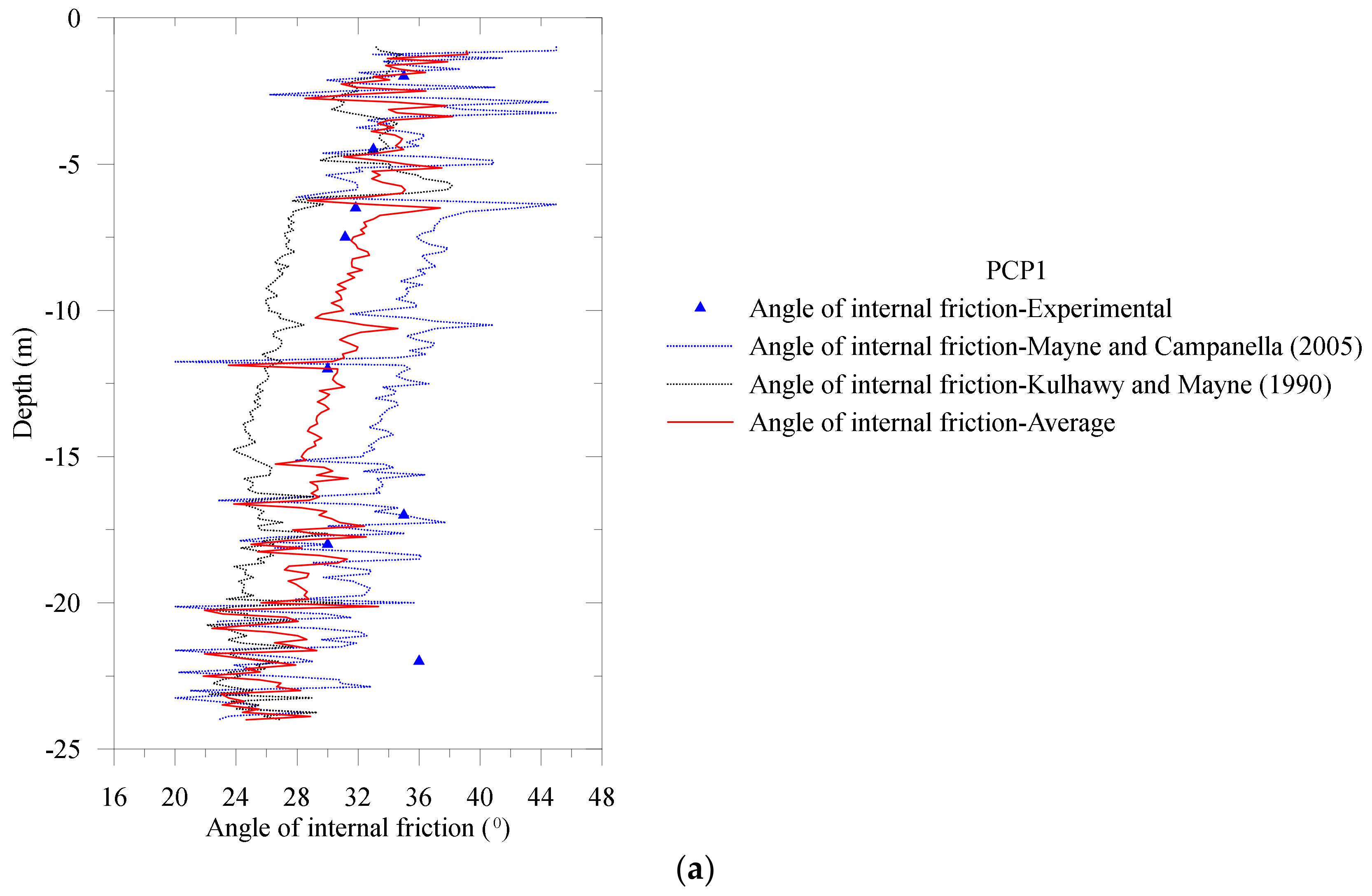
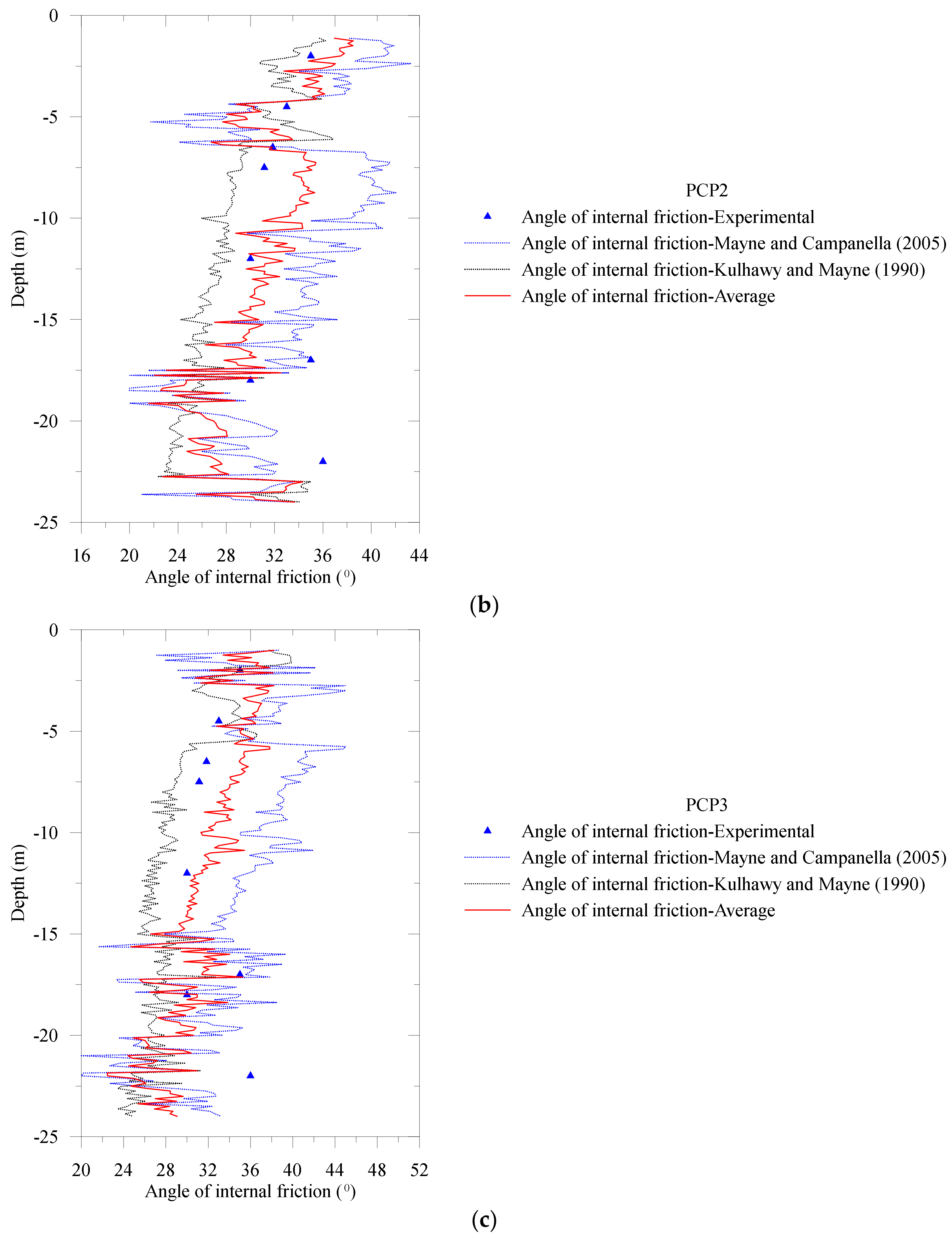
It is important to note that the critical state line slope (M) (see Roscoe and Burland [11]), is related to the internal friction angle . The relation between M and depends on many factors (see also Budhu [27]). For the axisymmetric compression, we find and for the axisymmetric extension (Roscoe and Burland [11]). First, is obtained from laboratory tests. Then, is also interpreted using CPT data. In this regard, following two procedures were considered.
Mayne and R.G. [28] presented as
where and are the total stress and the effective stress, respectively. and are the normalized parameters, which represent the ratio of the cone tip resistance and the pore pressure, respectively. is the hydrostatic pore water pressure, while is the generated pore water pressure behind the cone tip resistance (see also Figure 3). The expression of and was defined earlier.
Kulhawy and Mayne [29] obtained as
where and are the normalized cone tip resistance and the normalized friction ratio, respectively. It is worth mentioning that if (see Equation (5)).
Two types of CPT interpretations for (see Equations (4) and (7)) are presented in Figure 8. For the NBR clay deposit, the Mayne and R.G. [29] method overpredicted the angle of internal friction, while Kulhawy and Mayne [29] underpredicted . However, it is found from Figure 8 that the average of these two methods (see Equations (4) and (7)) is nearly identical to the experimentally measured angle of internal friction.
The lateral earth pressure (see also Michalowski [30]) for the normally consolidated (NC) clay (see Jaky [31]) and the over consolidated (OC) clay (see Mayne and Kulhawy [32]) are written as
In Equation (13), the OCR represents the over consolidation ratio, which is the ratio of the preconsolidation pressure and the present effective vertical stress . The interpretation of using the CPT data is presented as follows
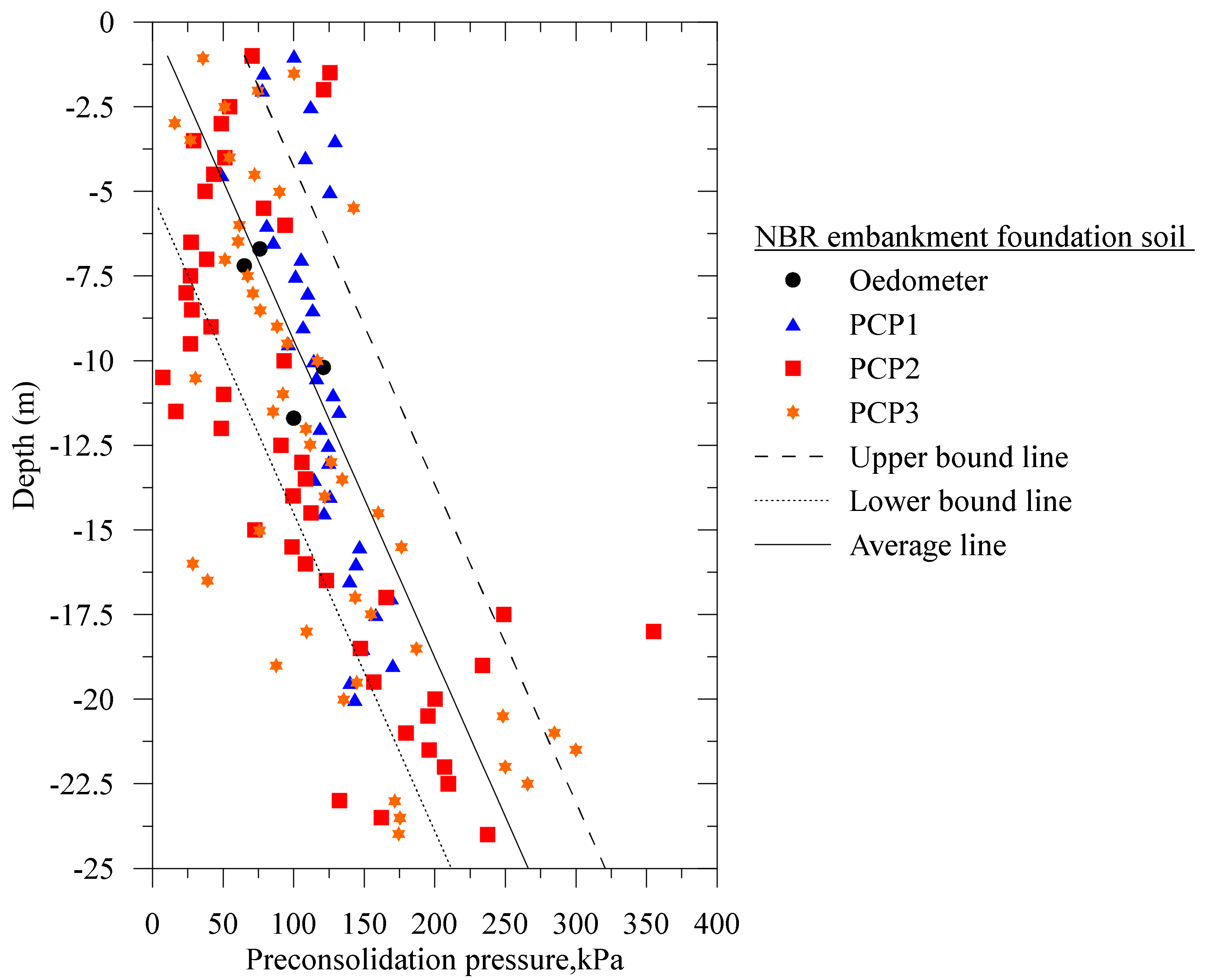
Undisturbed soil samples were collected to obtain the preconsolidation pressure at depths of RL = −6.50 to −6.90 m, RL = −7.00 to −7.40 m, RL = −10.00 to −10.40 m and RL = −11.50 to −11.90 m. Soil samples of these layers represent silty clay-1, silty clay-2, and silty clay-3, respectively. The oedometer test were performed on undisturbed samples. A comparison of the laboratory obtained preconsolidation pressure and CPT interpreted values are presented in Figure 9. We used PCP1, PCP2, and PCP3 data (see Figure 3) for CPT data interpretations. Additionally, Mayne and Brown [33] proposed CPT interpretation for as follows
where is the small strain shear modulus, and is obtained from Equation (10). An average line for was plotted from CPT interpreted values. The upper and the lower bound lines were plotted considering the single standard deviation of the average line as illustrated in Figure 9. It is observed that the oedometer test data were in between two bound lines.
Mayne [24] stated that the cohesion intercept is 2.0% of and zero, respectively, for the short time loading and the long-term loading. Robertson and Cabal [23]; Mayne [24] reported a co-relation for the undrained shear strength as
where is the bearing capacity factor which depends on many conditions including the loading direction, stress state, strain rate, boundary conditions, and sample disturbances (see also Mayne [24]). Therefore, it is challenging to obtain a unique correlation for from CPT interpretation. Robertson [34] presented the expression of as follows
Also, Budhu [27] presented an expression for based on the plasticity index (PI) greater than 10.0. Vesic [35] presented a correlation for considering the rigidity index of soil. In addition, assuming , Robertson and Cabal [23] presented the following:
was defined in Equation (5). Assuming that the sleeve friction measures the remolded shear strength , we find (see also Robertson and Cabal [23])
The CPT interpreted soil sensitivity is obtained from Equations (16) and (18) as (see Robertson and Cabal [23])
was presented earlier in Equation (11). Robertson and Cabal [23] reported that the value is too low for . Therefore, CPT interpretation for may not provide accurate results for highly sensitive clay (see also Robertson and Cabal [23]).
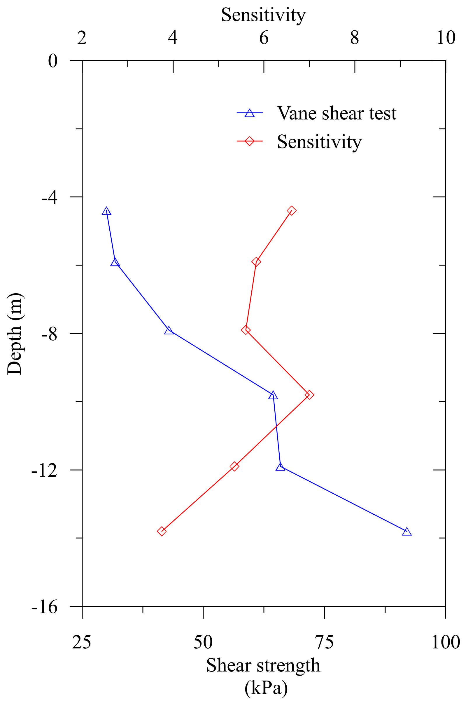
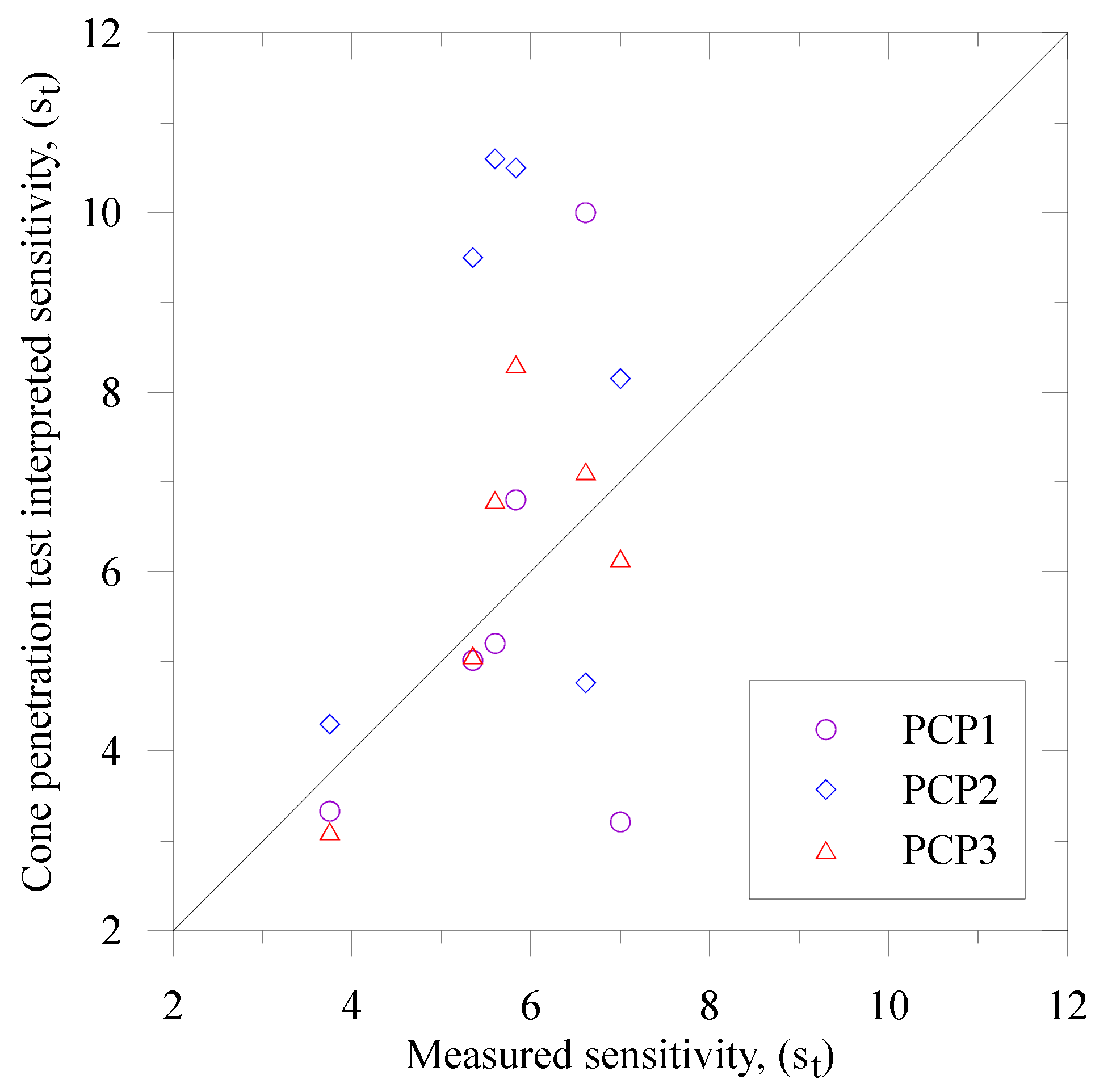
On the other hand, the undrained shear strength was obtained from the vane shear tests at depths of 4.40 m, 5.90 m, 7.90 m, 9.80 m, 11.90 m, and 13.80 m. The maximum undrained shear strength ranged from 30.0 kPa to 92.0 kPa. Also, the NBR embankment foundation’s sensitivity was calculated from the ratio of the undrained shear strength of the in-situ test to the remolded test. The sensitivity ranged from 3.75 to 7.0. The measured undrained shear strength and the sensitivity of the NBR embankment’s clay deposits are presented in Figure 10.
A comparison of the measured sensitivity of the NBR embankment foundation clay and the CPT interpreted values are demonstrated in Figure 11.
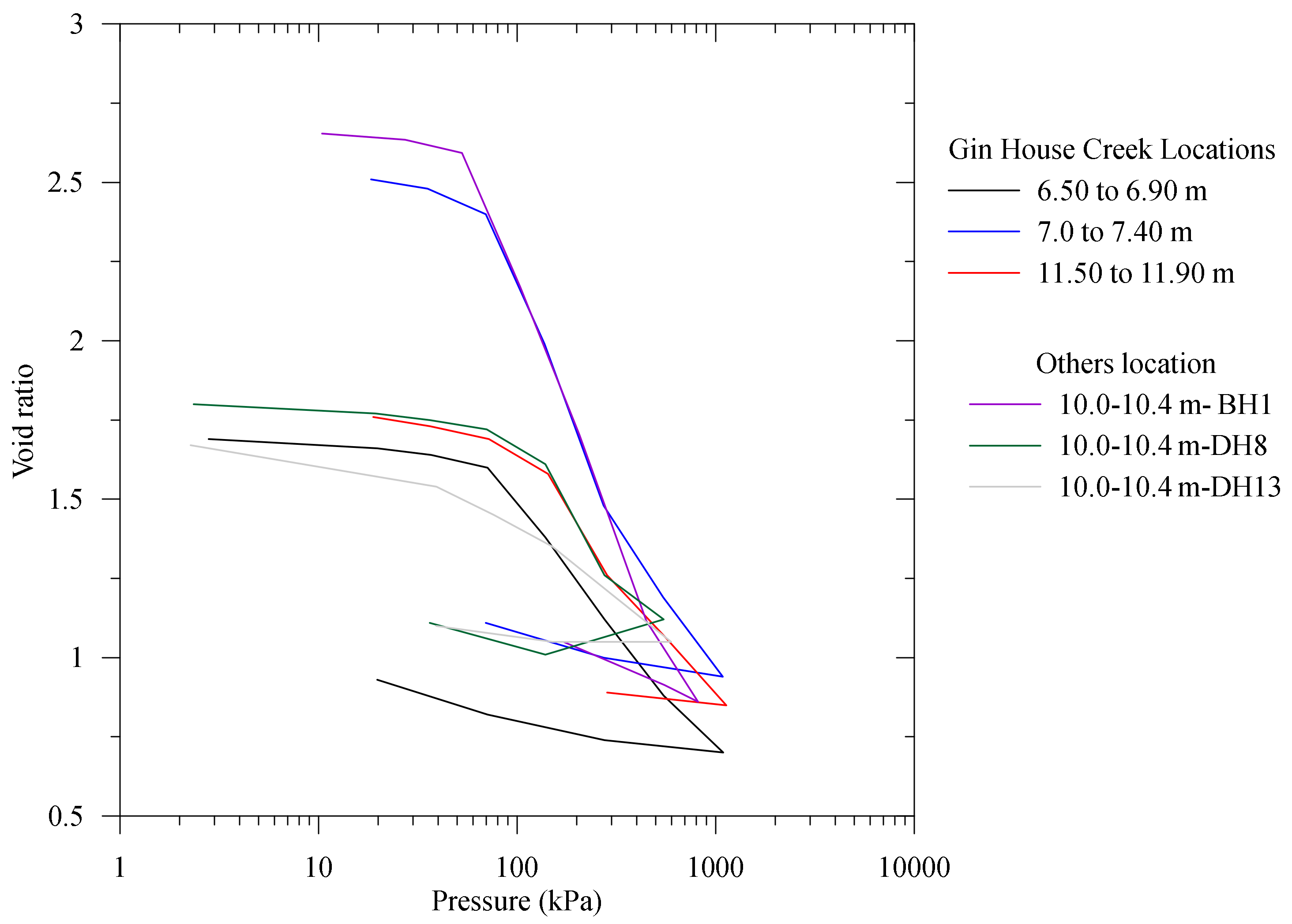
The oedometer tests were performed using 24 h load steps to measure the consolidation properties. The consolidation tests result of the NBR embankment’s clay deposit are presented in Figure 12. It is observed that the ratio of and in Figure 12 are not constant and change with the soil layer depth. Here, , and are the compression index, the swelling index, and the initial void ratio.
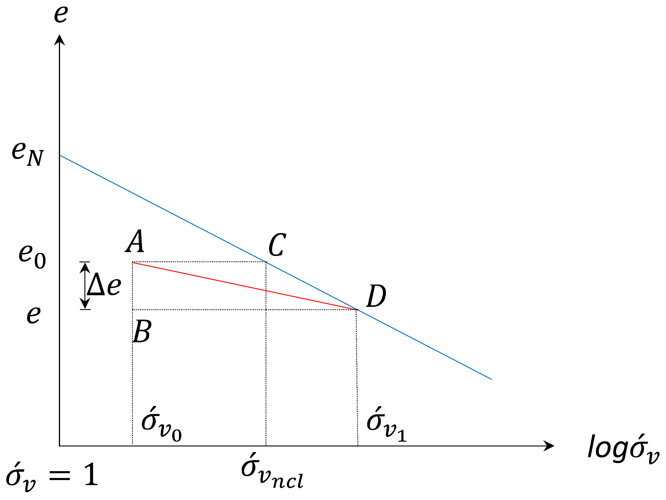
The fundamental structure of the elasto-viscoplastic models’ formulation is presented in Figure 13 (see Islam and Gnanendran [8]), while and are two model parameters, which can be either obtained from the laboratory tests or the CPT interpretation as below.
The coefficient of volume decrease , and are presented as
where, is the volumetric strain, is the effective vertical stress, is the void ratio, while demonstrates the change of quantities.
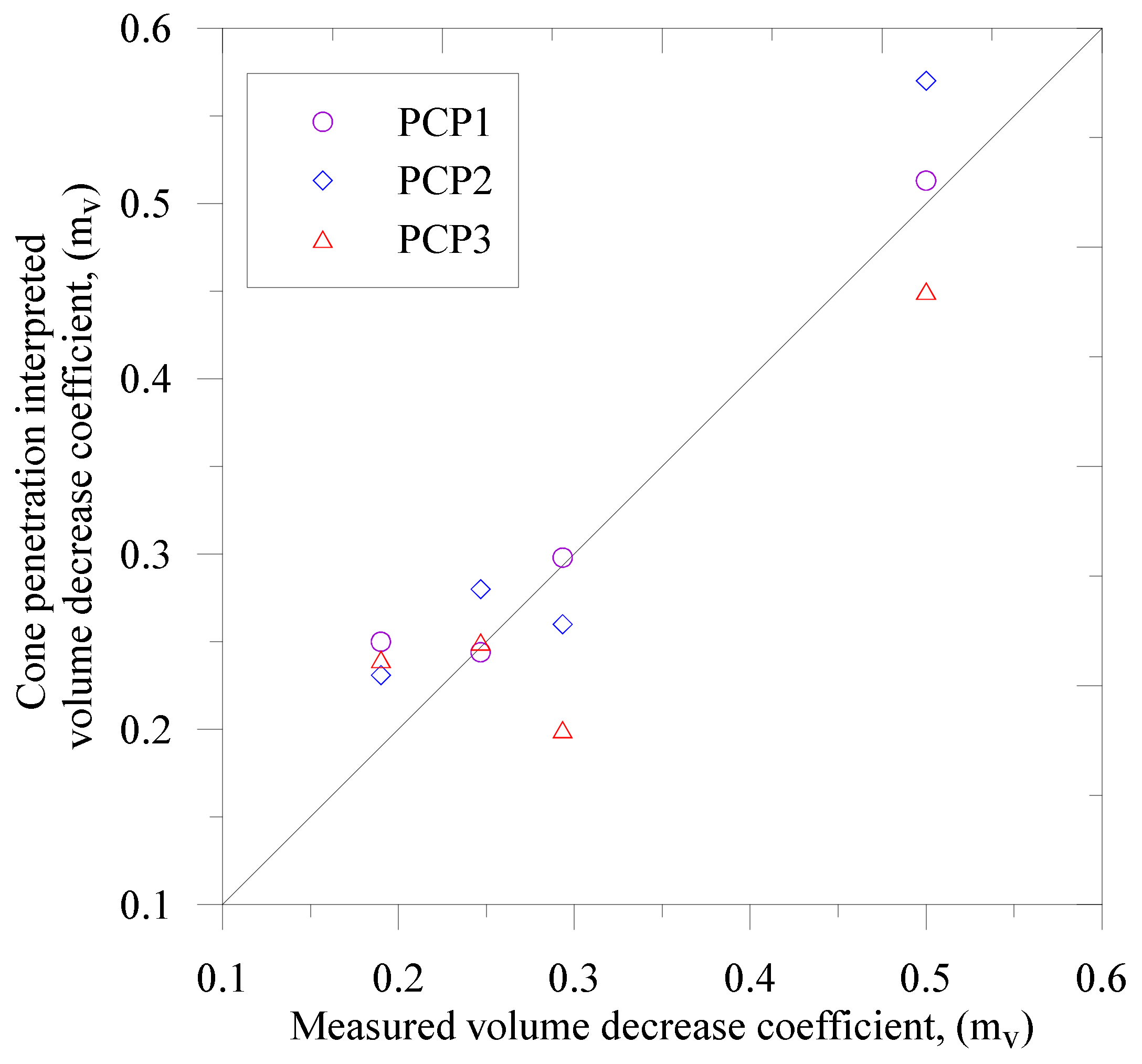
Using CPT relation, it is challenging to obtain the initial void ratio in Equation (21)–(23) for the in situ condition. Therefore, CPT interpreted is used herein to calculate and . Along the loading and unloading line is known as the compressibility index and the recompressibility index. Robertson and Cabal’s [23] proposed method is used to deduce with respect to the constrained modulus as follows
In Equation (24), depends on the soil behavior type index (see Equation (10)). For and , , while and , . Also, for , and relation can be obtained as (see also Robertson [25]).
A comparison of the laboratory measured and CPT interpreted are presented in Figure 14, which shows relatively good agreement. Robertson [34] also provided a correlation for and considering for . However, for the NBR embankment foundation, such a correlation underpredicts the experimentally measured and values. In this regard, Robertson [34] reported that based CPT relationships for and require additional improvement with respect to soil properties (e.g., plasticity index, moisture content).
The viscous property of soft clay, e.g., the secondary compression index, dominates the creep phenomena. Hence, it is important to incorporate the viscosity of clay in the finite element model formulation to foresee the time dependent performance of roadway embankments like the NBR embankment. There are several definitions available in the literature for (see also Liingaard et al. [16]). For example, and where e is the current void ratio; represents the initial void ratio; t is the time; demonstrates the vertical strain; and are the secondary compression index in terms of the void ratio and the strain. For the long-term prediction of soft clay’s viscous behavior, it is important to calculate precisely. In this regard, there are several methods available in the literature to obtain . Examples include: (i) an experimental method using the oedometer test or triaxial test (see Liingaard et al. [16]); (ii) empirical relations obtained from experiments (see Mesri and Castro [36]); and (iii) interpretations using cone penetration tests (see Tonni and Simonini [37]). We followed all three methods for the NBR embankment.
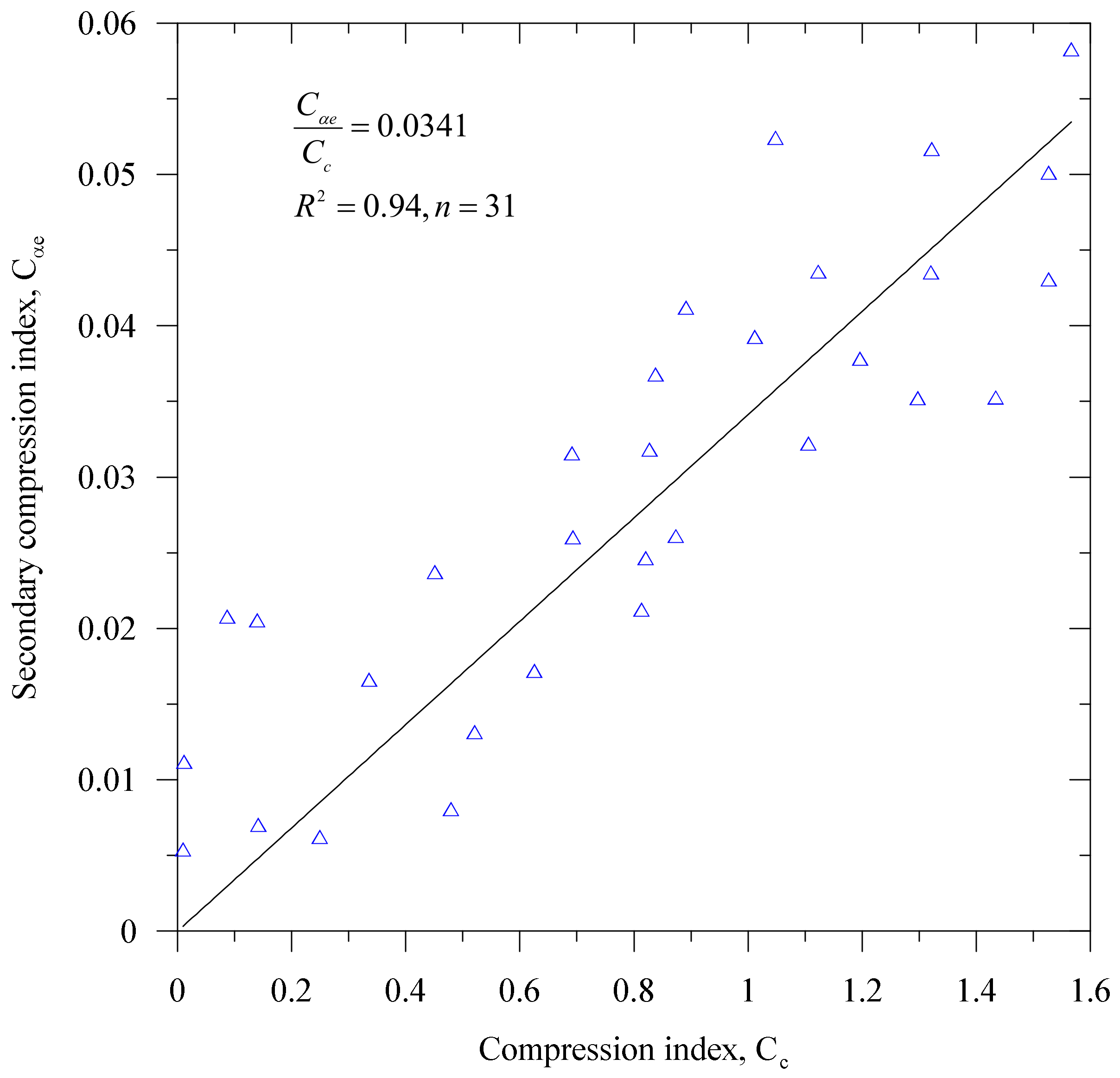
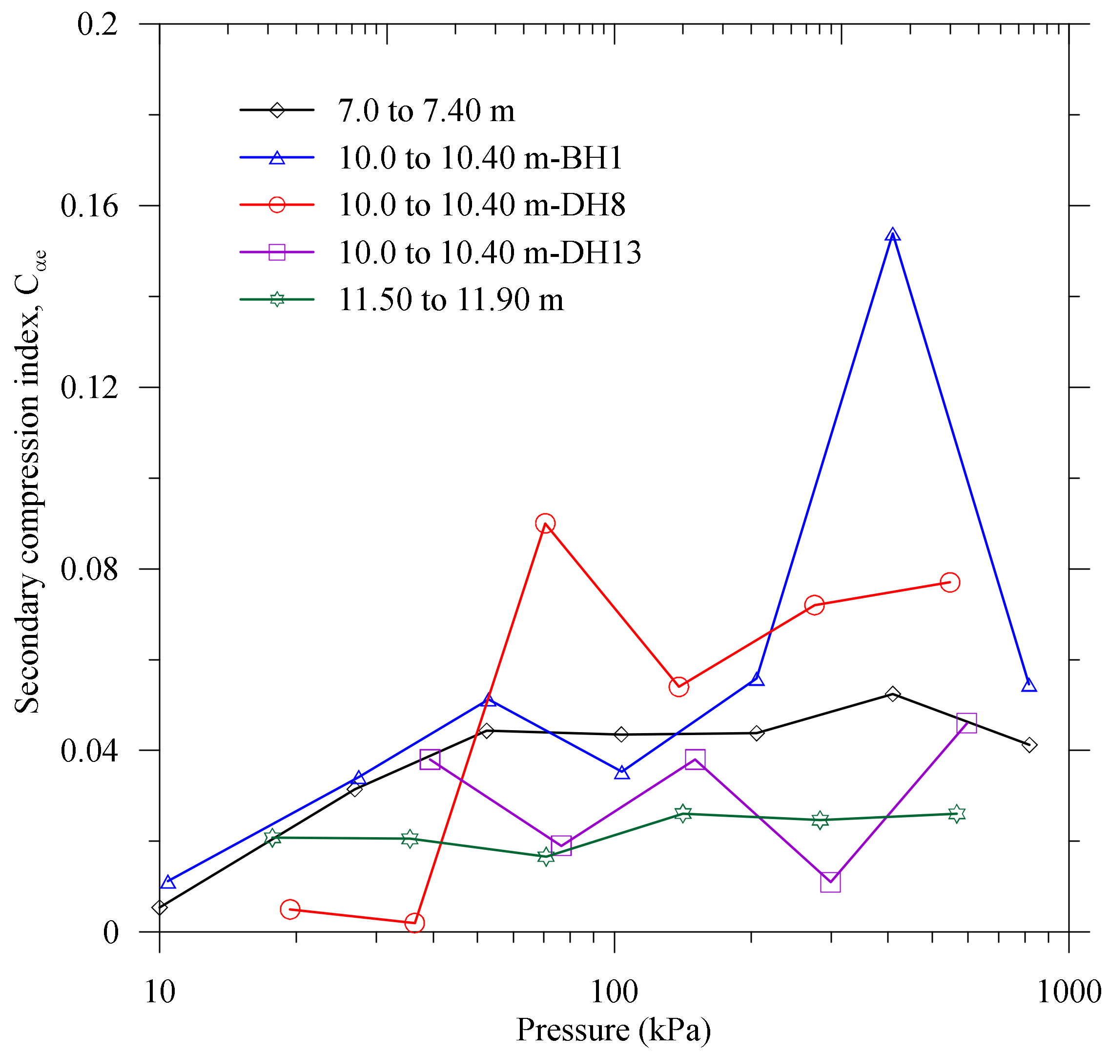
The laboratory measured and relationship for the NBR embankment foundation clay is presented in Figure 15. It is observed that may increase, decrease, or remain constant with the increase of applied load. Also, ratio for the NBR embankment foundation is 0.0341 , which supports Mesri and Castro [36]. The dependency of on the stress state is presented in Figure 16.
Among others, Tonni and Simonini [37] presented the following CPT interpretation for
where a and b are constants which can be obtained from the best plot data of measured from experiments and the interpretation obtained from CPT data. is defined in Equation (8). For the NBR embankment foundation, a and b in Equation (25) are 0.303 and −0.203, respectively. The and relation for the NBR embankment soils is illustrated in Figure 17.
Again, the coefficient of consolidation in the horizontal direction is presented as (see Teh and Houlsby [38])
values for the piezocone and the piezocone are 0.118 and 0.245, respectively (Teh and Houlsby [37]); is the radius of the piezocone (35.7 mm); and represents the time for 50% dissipation, which is obtained following the root-time plot method (see Sully and Campanella [39]). values for the NBR embankment foundation’s soil are presented in Table 1. is the rigidity index, which is deduced using the critical state soil mechanics theory as below (see Kulhawy and Mayne [29]).
where is the critical state line slope (see also Roscoe and Burland [11]), is the initial void ratio, OCR is the over consolidation ratio. , and OCR are obtained from the triaxial tests. , and are presented in Figure 12.
Robertson [34] presented a simplified relation for as follows
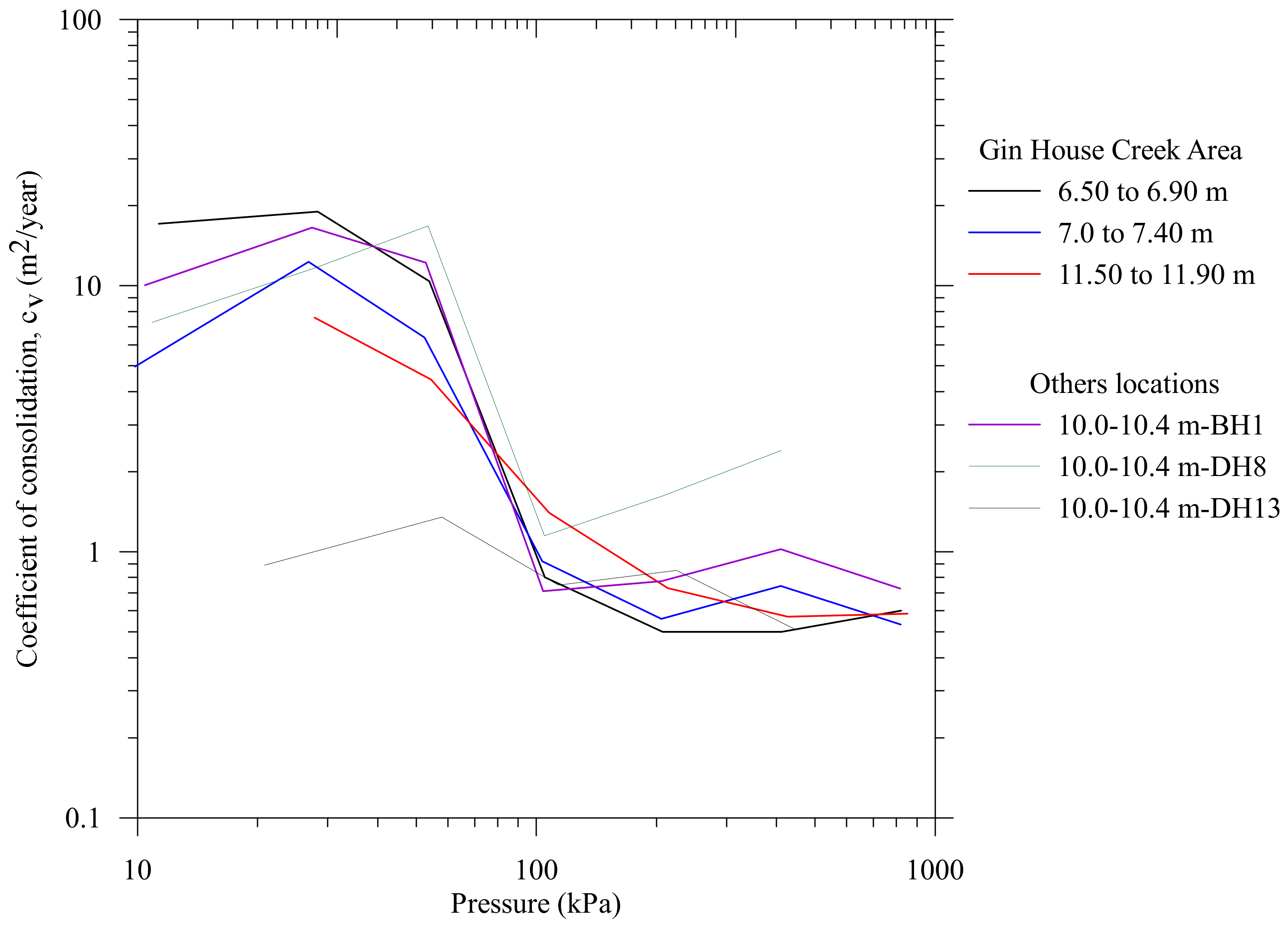
The units for and in Equation (28) are m2/sec and minutes. The coefficient of consolidation in the vertical direction is obtained from the laboratory tests and demonstrated in Figure 18.
The coefficient of horizontal permeability and (see Equation (26)) are presented as (see Robertson and Cabal [23])
where is the unit weight of water. and are discussed in Equations (28) and (24), respectively.
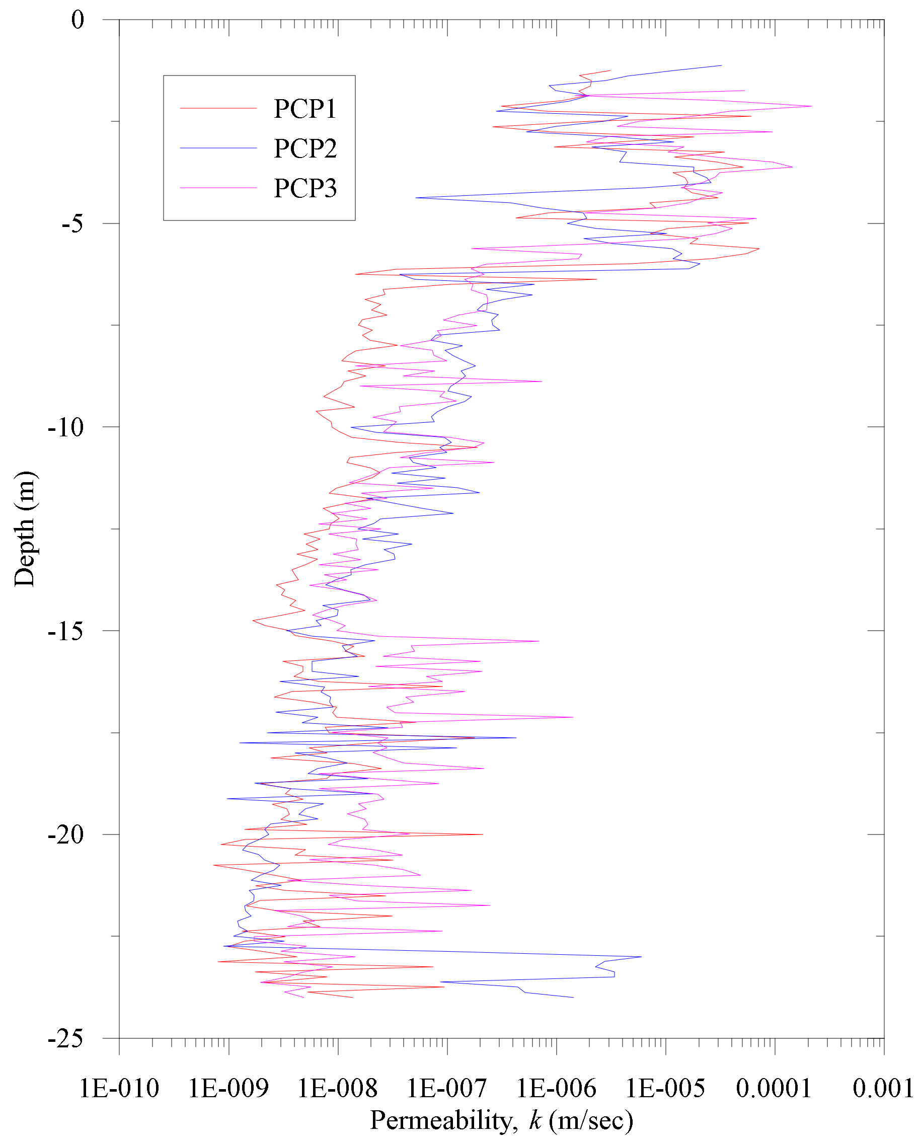
A relation between the soil permeability and (see Equation (10)) is also presented as follows (see Robertson and Cabal [23] and Figure 19):
A permeability profile of the NBR embankment foundation using CPT data is presented in Figure 19. Among others, Robertson and Cabal [23] demonstrated that for the isotropic compressibility, the ratio of the consolidation coefficient in the horizontal to the vertical is similar to the coefficient of permeability ratio in the same direction. Thereby, for known values of , and , the vertical permeability coefficient is obtained. Robertson and Cabal [23] presented benchmark values of for geomaterials. In the literature, there is another approach named the “back analysis” to obtain the ratio of or from the measured fitting data for settlement (see Karim et al. [13]).
5. Finite Element Modeling
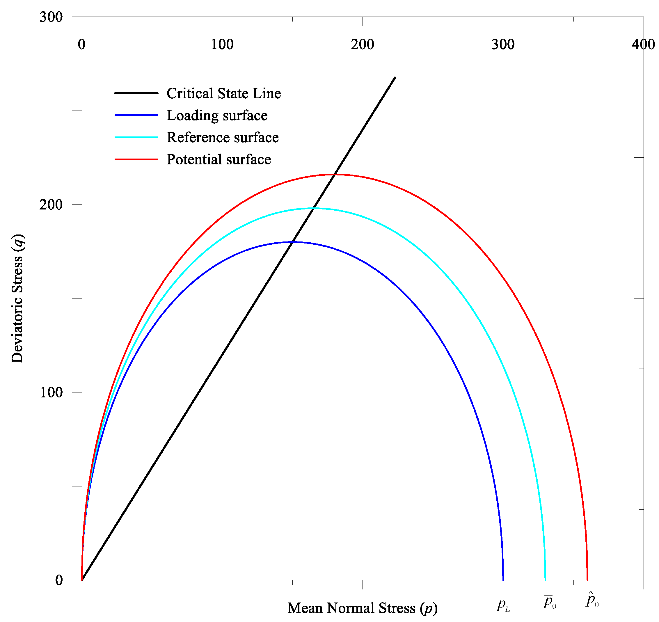
For the finite element simulation of the NBR embankment sections, we developed two fully coupled consolidated nonlinear elasto-viscoplastic models (EVP). In this regard, we considered the associated and the non-associated flow rule (Islam and Gnanendran [8]; Islam et al. [9]; Islam and Gnanendran [10]). To formulate EVP models, we considered the critical state theory (Roscoe and Burland [11]), the bounding surface theory (Dafalias [40]), and Perzyna’s overstress theory [41]. The NAFR based EVP model requires three surfaces (see also Appendix A). They are the potential surface , the reference surface , and the loading surface . In Appendix A, we present details of surfaces (see Figure A1). We also obtain the associated flow rule (AFR) EVP model assuming that and are identical.
The number of EVP model parameters is six, which is divided into the MCC model parameters and the secondary compression co-efficient . The MCC model parameters are divided into three: (i) the consolidation parameters, viz., the normal consolidation line slope , and the swelling line slope (see Figure 13); (ii) the strength parameter, viz., the critical state line slope (M); and (iii) elastic parameters, viz., Poisson’s ratio and the Young’s modulus, . We obtain the void ratio at unit mean pressure in the mean pressure and the void ratio space from the triaxial test or the oedometer test (see Figure 13). We considered the void ratio based as the initial value for the finite element analysis. We introduced a generalized non-linear function as follows (see Islam and Gnanendran [10])
where and are the secondary compression index at the known reference stress state and the current stress state, while .
Moreover, we incorporated both EVP models in a numerical solver named a finite element numerical algorithm (AFENA) [42]. We introduced the large deformation analyses (LDA) (see Carter et al. [43]) to update nodal coordinates at the end of every load increment. We present the EVP models in Appendix A. We demonstrate the EVP model parameters of the NBR embankment section in Table 2.
In this paper, we discussed the procedure to obtain EVP model parameters from CPT interpretation which is a new contribution compared to our previous papers. In this regard, we also compared CPT interpreted EVP model parameters with the laboratory measured values. Both EVP models were developed considering the MCC equivalent surface to compare the MCC model prediction with EVP model. The objective of such comparison is to investigate the effect of clay’s viscosity in the long-term monitoring of the NBR embankment. Also, the purpose of two EVP models is to assess the flow rule effect of the natural soft clay
We demonstrate the NBR embankment’s finite element (FE) geometry in Figure 20. We also illustrate the construction history of the embankment sections in Figure 21. The embankment’s length, width, and depth are 1.63 km, 20.0 to 28.0 m, and 5.0 to 21.0 m, respectively. After initiation of geostatic conditions, we followed the staged construction procedure (see Figure 21) for numerical simulation of the embankment. We assumed that the outer vertical boundary and the bottom boundary were impermeable for the coupled FE solutions. We extended the NBR embankment’s width and depth to 1.5 times on each side to minimize the boundary effect. For the FE discretization, we used six node nonlinear triangular elements. Besides, we applied the load incrementally to simulate the NBR embankment’s construction history and to avoid the numerical convergence instabilities.
We assumed Poisson’s Ratio = 0.30, ; ; is the initial void ratio.
We used two EVP models and the MCC model to characterize clay deposits of the NBR embankment foundation for the coupled FE solutions. In addition, we considered the Mohr–Coulomb model for the embankment’s fill materials, the foundation’s sand layers, and the argillite bedrock. In this paper, we compare field observed data obtained from settlement plates and piezometers with the EVP models and the MCC model predicted responses.
In the next section, we present observed and predicted responses.
6. Comparison of Observed and Predicted Responses
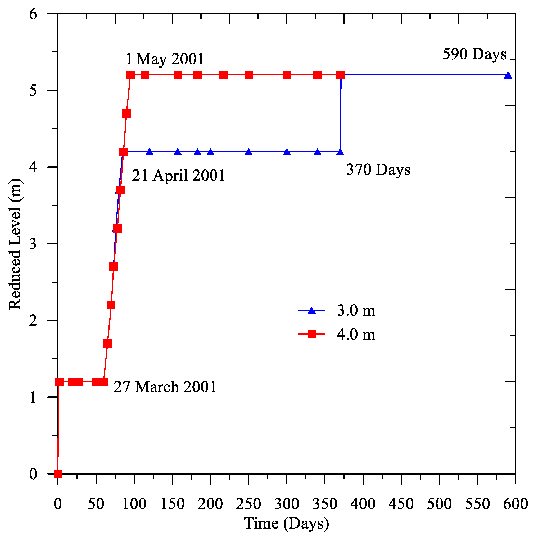
The QDTMR installed 18 settlement plates and three piezometers in December 1999 in the vicinity of the Gin House Creek location of the NBR embankment to measure settlement and pore pressure (see also Figure 2). The Creek area is considered as a problematic zone due to the presence of organic components and compressible clay deposits. Therefore, the QDTMR has applied three measures considering the location and the subsurface conditions to avoid stability problems. They are: (i) 3.0 m preloading, (ii) 3.0 m preloading and 1.0 m surcharging, and (iii) 4.0 m preloading. It is worth mentioning that the 3.0 m preloading height section was monitored for 370 days. Then, 1.0 m surcharge was applied, and additional monitoring continued to 590 days (see Figure 21). The 4.0 m preloading embankment section was monitored for 390 days. The QDTMR started the surcharged-preloading in February 2000.
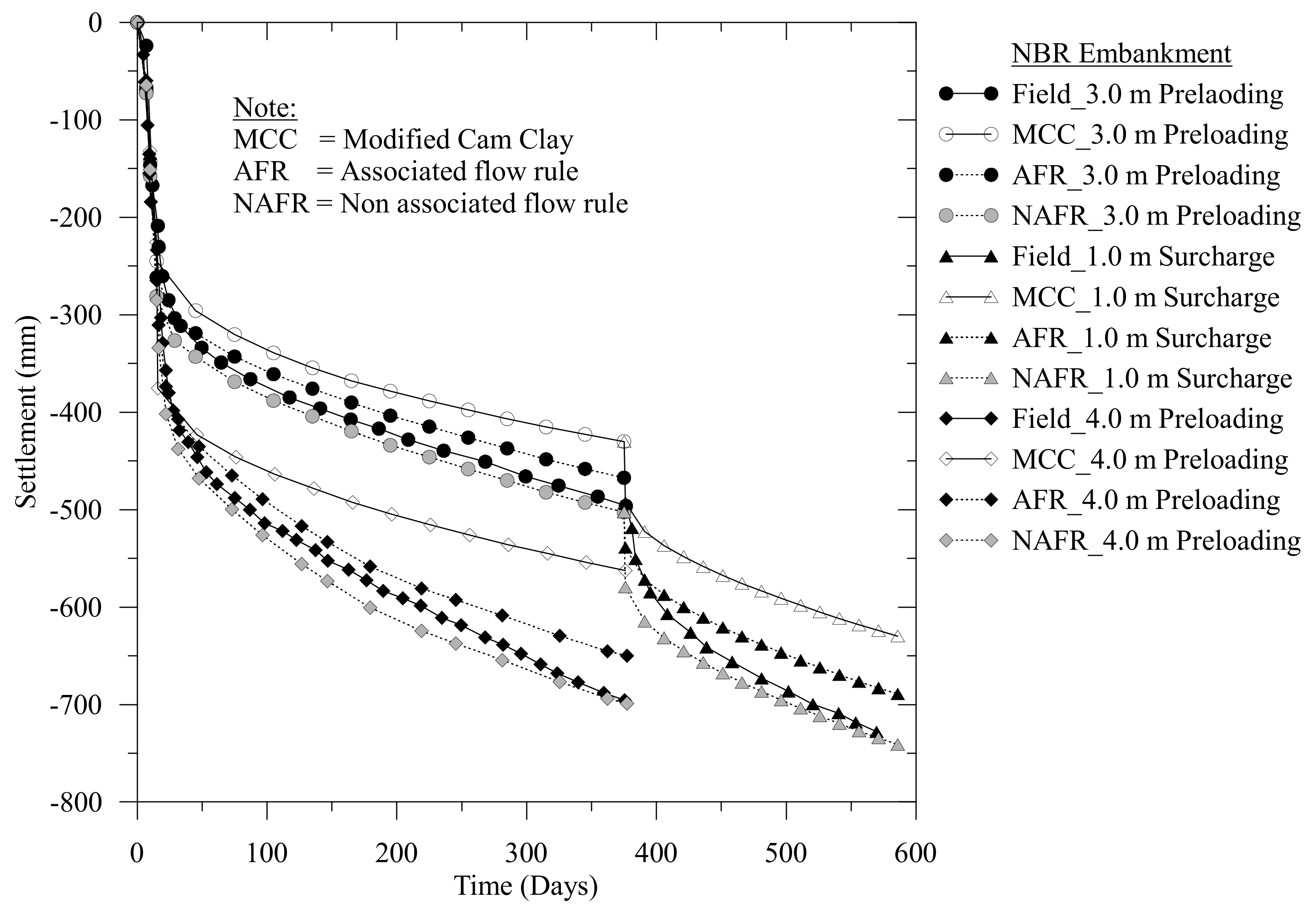
We performed FE simulations using EVP models and the MCC model to predict the NBR embankment foundation’s long-term behavior. In this paper, we limit our coupled FE model comparisons to data from three settlement plates and three piezometers, considering the available field data and the laboratory experiments on the undisturbed samples. We observed that the MCC model predicted the measured settlements for both preloading and surcharging until 60 days (see Figure 22) of the NBR embankment’s construction time. Then, the MCC model started to underpredict the observed settlement. For 3.0 m preloading, the underprediction in the MCC model after 370 days was 13.30%. The underestimation in the MCC model developed as the MCC model formulation is incapable of modeling the long-term viscous behavior of soft clay. We formulated the EVP models to account for the creep of soil.
Islam and Gnanendran [10] proposed that the viscoplastic component of strain increment (see Equation (A4) in Appendix B) is normal to the plastic potential. Therefore, when is calculated by assuming the AFR, where the potential surface and the reference surface are the same (see Figure A1), the predicted settlement is lower than in the NAFR model. In this regard, Islam and Gnanendran [10] also presented the importance of the NAFR (see also Hashiguchi [18]) over the AFR considering the stress-dilatancy relation.
From the comparison of the observed and predicted settlement response of 3.0 m preloading, we found that after 370 days, the underprediction in the AFR based EVP model was 3.78%. In contrast, for identical conditions, the NAFR based EVP model overpredicted 1.12%. We also noticed a similar prediction in the MCC model and EVP models for 1.0 m surcharging and 4.0 m preloading. Also, for 3.0 m preloading, the underprediction in the AFR EVP model and the MCC model was relatively high compared to surcharged-preloading and 4.0 m preloading which might be due to changes of the stress state during the increase of the height of the fill material.
After 590 days for 1.0 m surcharging, we noticed that the underprediction in the MCC model and the AFR based EVP model was 14.25% and 4.5%, respectively, while the over-prediction in the NAFR based model was negligible. After 370 days for 4.0 m preloading, we observed 20.0% and 5.0% underprediction in the MCC model and the AFR based EVP model, respectively. In contrast, for similar preloading and duration, the NAFR based EVP model prediction was reasonably good. We also observed that the MCC model did not capture time dependent viscous behavior of the NBR embankment’s soft clay.
For the NBR embankment foundation, the NAFR based EVP model well captured measured settlement compared to the AFR based EVP model. We thus observed the flow rule effect for the NBR embankment foundation’s natural soft clay. Moreover, from comparisons of triaxial test results and EVP model predictions, Islam et al. [9] and Islam and Gnanendran [10] reported a similar flow rule effect for the undisturbed natural soft clay (e.g., the Osaka clay, the Shanghai clay, and the San Francisco Bay Mud).
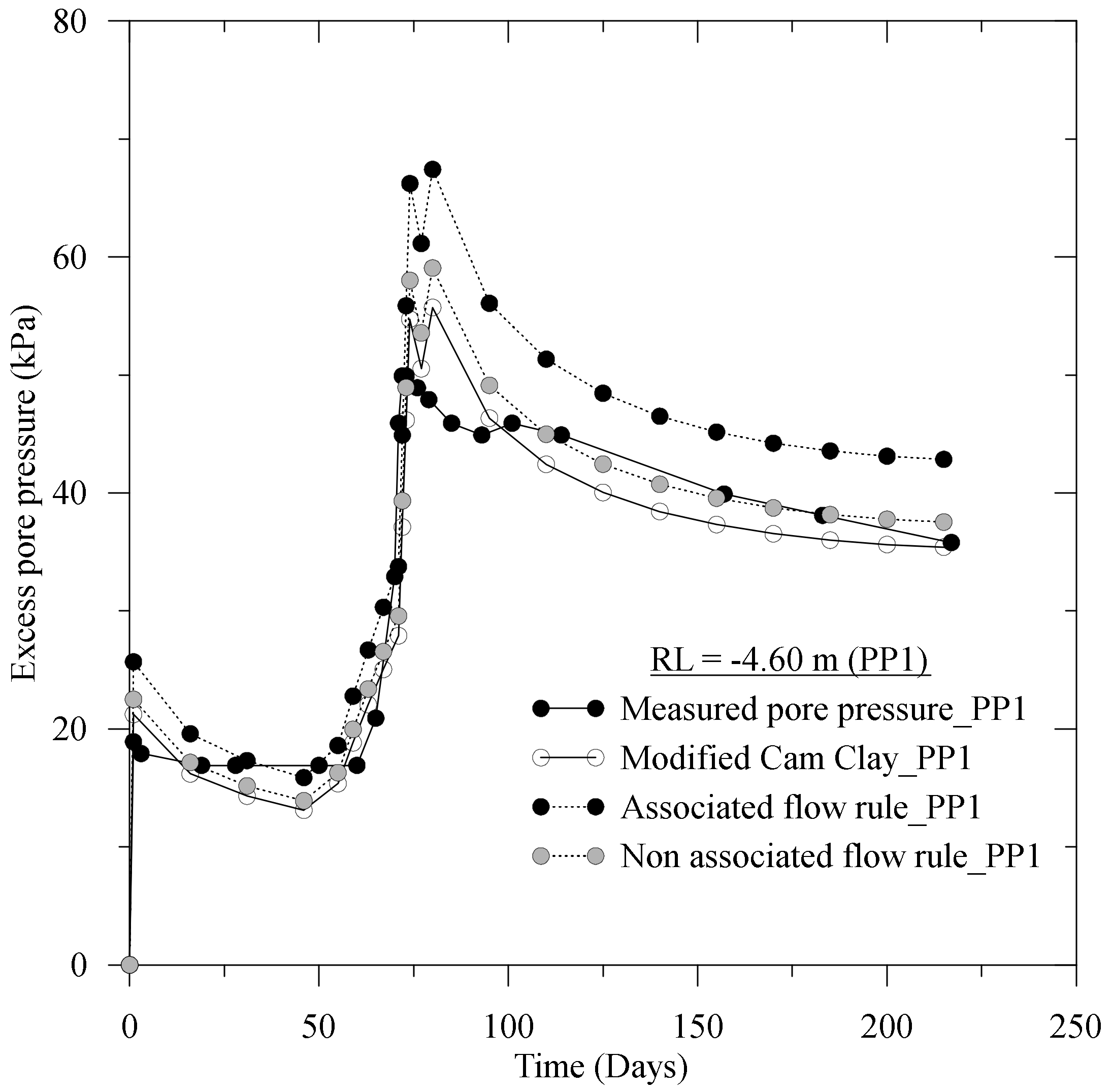
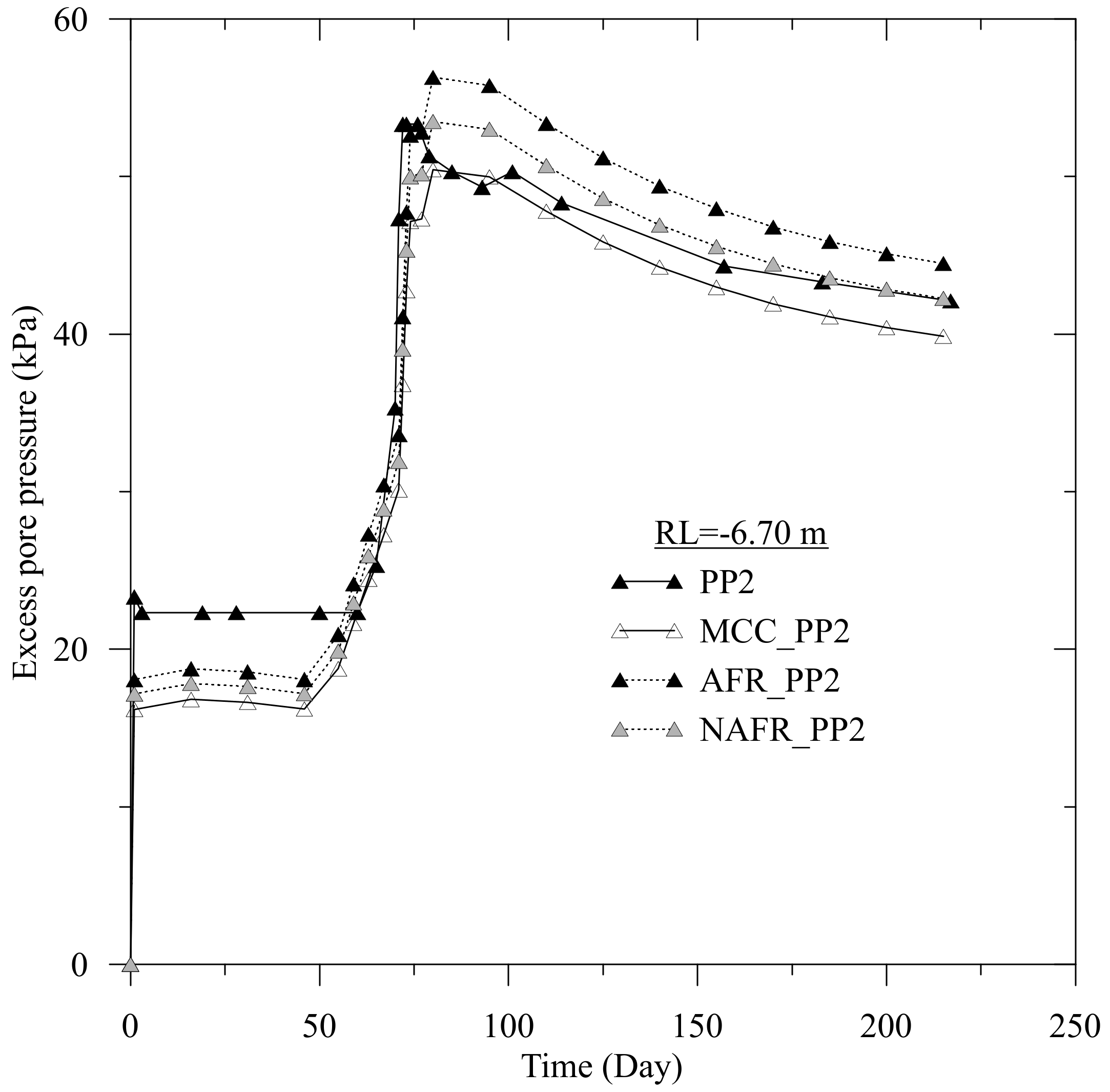
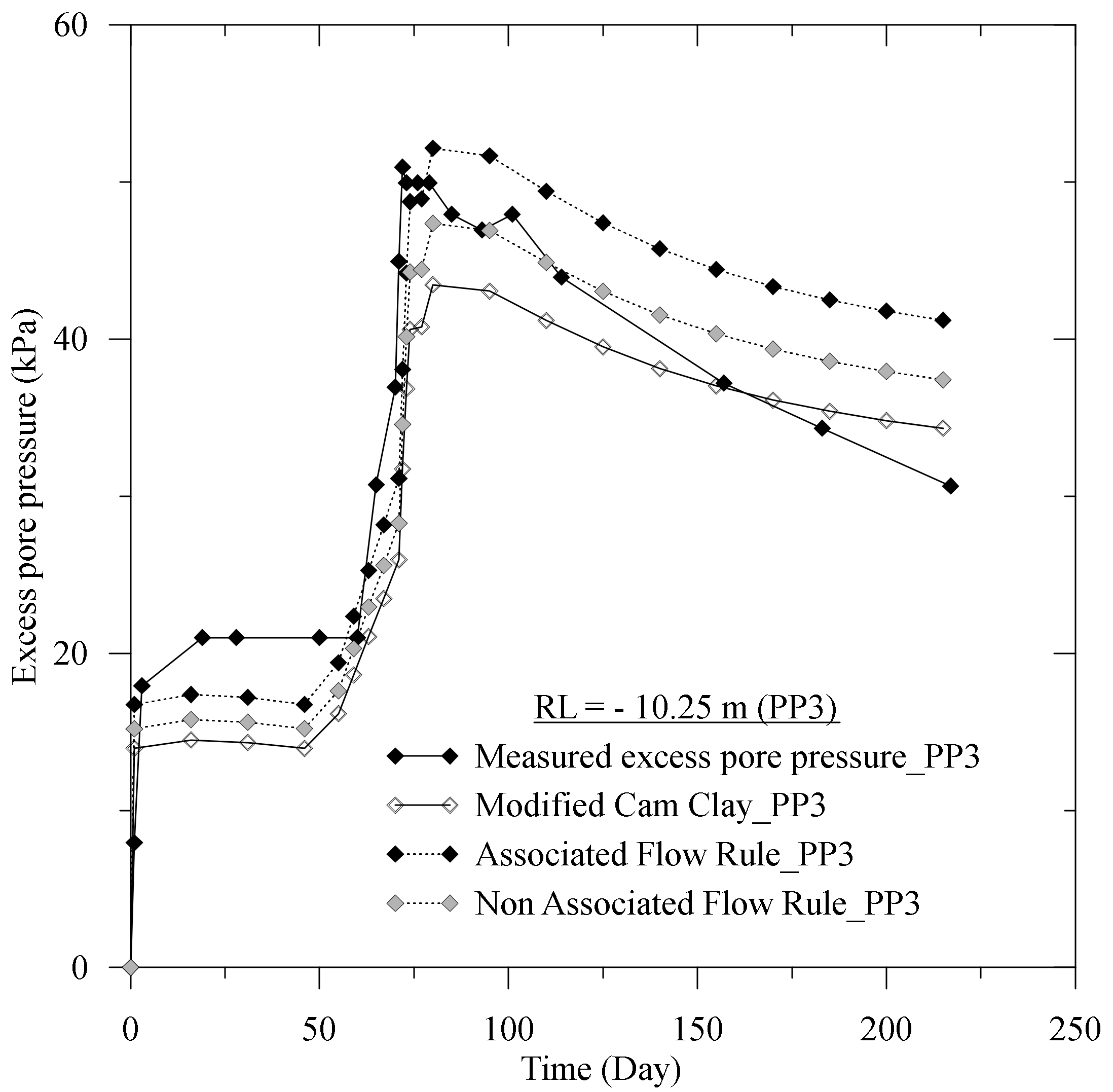
In the NBR embankment’s 4.0 m preloading section, the QDTMR installed a total of three piezometers at the reduced level (RL) = −4.60 m, −6.70 m, and −10.25 m for 217 days. The QDTMR installed these piezometers to measure the excess pore water pressure (EPWP) responses of the NBR embankment. We presented the observed and predicted EPWP responses in Figure 23, Figure 24 and Figure 25.
During the construction period, the NAFR EVP model underpredicted the measured EPWP at RL = −4.60 m, then the model overpredicted the EPWP, as is illustrated in Figure 23. After the peak EPWP, the MCC model underpredicted the EPWP, while the AFR based EVP model overpredicted the EPWP. We observed that the finite element model predictions obtained from the EVP models and the MCC model followed an identical pattern for the piezometers at RL = −6.70 and −10.25 m, as presented in Figure 24 and Figure 25, respectively. We also noticed a variation in the models’ prediction for the piezometer at RL = −10.25 m (see Figure 25). This might be due to the deviation of the piezometer from the midpoint location and the increase of non-verticality.
7. Conclusions
In this paper, we presented details of the NBR embankment’s geology, subsurface, and geotechnical properties. We obtained the embankment’s subsurface profile from field boreholes data comparing them with CPT and CPT-u tests interpreted data. We also correlated the laboratory measured geotechnical data with CPT and CPT-u calculated data, demonstrating reasonably good agreement of measured and calculated geotechnical properties. We used CPT, CPT-u, laboratory, and field monitoring data to stratify the NBR embankment foundation, which we also used for the coupled FE simulations. Moreover, we found from the settlement plates data that the surcharged-preloading was effective for the NBR embankment foundation for the identical height of preloading only.
We presented two elasto-viscoplastic models assuming the associated and the non-associated flow rules. We compared measured settlement plates data with the EVP models, and the MCC model predicted responses. We observed that the MCC model underpredicted the long-term responses of soft clay settlement due to its time dependent viscous nature, while the NAFR EVP model captured the measured data well. We also observed the effect of the flow rule and the viscosity when predicting the excess pore water pressure (EPWP): the NAFR EVP model predicted the measured EPWP reasonably well.
Author Contributions
Conceptualization, M.N.I. and C.T.G.; methodology, M.N.I.; software, M.N.I. and C.T.G.; validation, M.N.I.; formal analysis, M.N.I.; investigation, M.N.I. and C.T.G.; resources, C.T.G. and S.T.S.; data curation, M.N.I., C.T.G. and S.T.S.; writing—original draft preparation, M.N.I.; writing—review and editing, M.N.I. and C.T.G.; visualization, M.N.I.; supervision, C.T.G. All authors have read and agreed to the published version of the manuscript.
Funding
This research received no external funding.
Institutional Review Board Statement
Not applicable.
Informed Consent Statement
Not applicable.
Acknowledgments
The University of New South Wales (UNSW), Canberra, Australia, provided financial support during the first author research at the UNSW. Additionally, the Queensland Department of Transport and Main Roads (QDTMR) provided field data and undisturbed soil samples.
Conflicts of Interest
The authors declare no conflict of interest.
Appendix A. Surfaces of the Elasto-Viscoplastic Models
We required the following three surfaces for the NAFR based EVP model (see also Figure A1 and Islam et al. [9])
In Equations (A1)–(A3), ,
and are the loading surface, the reference surface and the potential surface respectively, while ,
and
are intersections of these corresponding surfaces with the p-axis (Figure A1). Also, represents the mean pressure and corresponds to the deviatoric pressure. M is the slope of the critical state line.
Figure A1.
Three surfaces of the NAFR based EVP model.

Appendix B. Strain rate of the Elasto-Viscoplastic Models
The strain rate tensor comprises of the elastic component and the viscoplastic component as follows
We obtain the elastic component in Equation (A4) as
where is the modulus of elasticity; is the Poisson’s ratio; is the effective stress tensor, and is the Kronecker delta. Additionally, using Perzyna’s [41] concept, we obtain the viscoplastic strain rate as
From Islam, Gnanendran and Massoudi [9], we obtain the expression of for the non-associated flow rule as
Additionally, in Equation (A6), using the chain rule for , we find
We obtain in Equation (A6), by combining Equations (A8) and (A16) as follows
where, .
References
- Bergado, D.T.; Anderson, L.R.; Miura, N.; Balasubramaniam, A.S. Soft Ground Improvement in Lowland and other Environments; ASCE Press: New York, NY, USA, 1996. [Google Scholar]
- Han, J. Principles and Practices of Ground Improvement; Wiley: Hoboken, NJ, USA, 2015. [Google Scholar]
- Barden, L. Consolidation of clay with non-linear viscosity. Géotechnique 1965, 15, 345–362. [Google Scholar] [CrossRef]
- Indraratna, B.; Chu, J.; Rujikiatkamjorn, C. Ground Improvement Case Histories:Embankments with Special Reference to Consolidation and Other Physical Methods; Butterworth-Heinemann: London, UK, 2015. [Google Scholar]
- Indraratna, B.; Chu, J. Ground Improvement-Case Histories; Elsevier: London, UK, 2005. [Google Scholar]
- Islam, M.N.; Gnanendran, C.T.; Sivakumar, S.T. Prediction of Embankments’ Time-Dependent Behavior on Soft Soils: Effects of Preloading, Surcharging, and Choice of Lab Versus Field Test Data for Soft Soil Parameters. In Ground Improvement Case Histories; Rujikiatkamjorn, B.I.C., Ed.; Butterworth-Heinemann: Oxford, UK, 2015; pp. 359–379. [Google Scholar] [CrossRef]
- Meena, N.K.; Nimbalkar, S.; Fatahi, B.; Yang, G. Effects of soil arching on behavior of pile-supported railway embankment: 2D FEM approach. Comput. Geotech. 2020, 123, 103601. [Google Scholar] [CrossRef]
- Islam, M.N.; Gnanendran, C.T. Elastic-Viscoplastic Model for Clays: Development, Validation, and Application. J. Eng. Mech. 2017, 143, 04017121. [Google Scholar] [CrossRef] [Green Version]
- Islam, M.N.; Gnanendran, C.T.; Massoudi, M. Finite Element Simulations of an Elasto-Viscoplastic Model for Clay. Geosciences 2019, 9, 145. [Google Scholar] [CrossRef] [Green Version]
- Islam, M.N.; Gnanendran, C.T. Non-associated Flow Rule based Elasto-Viscoplastic Model for Clay. Geosciences 2020, 10, 227. [Google Scholar] [CrossRef]
- Roscoe, K.H.; Burland, J.B. On the Generalized Stress-Strain Behavior of Wet Clay. In Engineering Plasticity; Heyman, J., Leckie, F.A., Eds.; Cambridge University Press: Cambridge, UK, 1968; pp. 535–609. [Google Scholar]
- Gnanendran, C.T.; Valsangkar, A.; Rowe, R.K. Case Histories of Embankments on Soft Soils and Stabilisation With Geosynthetics: Canadian Experience, Chapter 27. In Ground Improvement Case Histories; Elsevier: London, UK, 2005. [Google Scholar]
- Karim, M.R.; Gnanendran, C.T.; Lo, S.C.R.; Mak, J. Predicting the long-term performance of a wide embankment on soft soil using an elastic–viscoplastic model. Can. Geotech. J. 2010, 47, 244–257. [Google Scholar] [CrossRef]
- Indraratna, B.; Rujikiatkamjorn, C.; Ameratunga, J.; Boyle, P. Performance and Prediction of Vacuum Combined Surcharge Consolidation at Port of Brisbane. J. Geotech. Geoenviron. Eng. 2011, 137, 1009–1018. [Google Scholar] [CrossRef] [Green Version]
- Sivasithamparam, N.; Karstunen, M.; Bonnier, P. Modelling creep behaviour of anisotropic soft soils. Comput. Geotech. 2015, 69, 46–57. [Google Scholar] [CrossRef] [Green Version]
- Liingaard, M.; Augustesen, A.; Lade, P. Characterization of Models for Time-Dependent Behavior of Soils. Int. J. Geomech. 2004, 4, 157–177. [Google Scholar] [CrossRef]
- Zienkiewicz, O.C.; Humpheson, C.; Lewis, R.W. Associated and non-associated visco-plasticity and plasticity in soil mechanics. Geotechnique 1975, 25, 671–689. [Google Scholar] [CrossRef]
- Robertson, P.K. Soil classification using the cone penetration test. Can. Geotech. J. 1990, 27, 151–158. [Google Scholar] [CrossRef]
- Roads, M. Gooding’s Corner Geotechnical Investigation; Report: R1748; Main Roads of Queensland, Materials and Geotechnical Services: Brisbane, QLD, Australia, 1991. [Google Scholar]
- Roads, M. Additional Geotechnical Investigation, Nerang-Broadbeach Road, Gooding’s Corner; Report: R3161; Main Roads of Queensland, Transport Technology, Geotechnical and Geological Services: Brisbane, QLD, Australia, 1999. [Google Scholar]
- Roads, M. Preload Monitoring, Nerang-Broadbeach Road, Goodings Corner Deviation and Neilsens Roads Intersection; Report MR1822; Main Roads of Queensland, Transport Technology, Geotechnical and Geological Services: Brisbane, QLD, Australia, 2000. [Google Scholar]
- Roads, M. Additional Geotechnical Investigation for the Proposed Western RSS Wall Area, Nerang-Broadbeach Deviation, Gooding’s Corner; Report: R3233; Main Roads of Queensland: Brisbane, QLD, Australia, 2001. [Google Scholar]
- Robertson, P.K.; Cabal, K.L. Guide to Cone Penetration Testing for Geotechnical Engineering, 4th ed.; Gregg Drilling and Testing, Inc.: Signal Hill, CA, USA, 2010. [Google Scholar]
- Mayne, P.W. Cone Penetration Testing A Synthesis of Highway Practice, NCHRP Synthesis 368; Transportation Research Board: Washington, DC, USA, 2007. [Google Scholar]
- Robertson, P.K. Interpretation of cone penetration tests—A unified approach. Can. Geotech. J. 2009, 46, 1337–1355. [Google Scholar] [CrossRef] [Green Version]
- Hegazy, Y.A.; Mayne, P.W. Statistical Correlations between Vs and CPT Data for Different Soil Types. In Proceedings, Symposium on Cone Penetration Testing; Swedish Geotechnical Society: Linkoping, Sweden, 1995; Volume 2, pp. 173–178. [Google Scholar]
- Budhu, M. Soil Mechanics and Foundations, 3rd ed.; John Wiley & Sons, INC.: Hoboken, NJ, USA, 2011. [Google Scholar]
- Mayne, P.W.; Campanella, R.G. Versatile Site Characterization by Seismic Piezocone. In Proceedings of the 16th International Conference on Soil Mechanics and Geotechnical Engineering, Osaka, Japan, 12–16 September 2005; pp. 721–724. Available online: https://www.issmge.org/uploads/publications/1/22/STAL9781614996569-0721.pdf (accessed on 4 November 2021).
- Kulhawy, F.H.; Mayne, P.W. Manual on Estimating Soil Properties for Foundation Design; Cornell University: New York, NY, USA, 1990. [Google Scholar]
- Michalowski, R. Coefficient of Earth Pressure at Rest. J. Geotech. Geoenviron. Eng. 2005, 131, 1429–1433. [Google Scholar] [CrossRef] [Green Version]
- Jaky, J. The coefficient of earth pressure at rest. J. Soc. Hung. Archit. Eng. 1944, 78, 355–388. [Google Scholar]
- Mayne, P.W.; Kulhawy, F.H. K0-OCR relationships in soil. J. Geotech. Eng. 1982, 108, 851–872. [Google Scholar]
- Mayne, P.W.; Brown, D.A. Site characterization of Piedmont residuum of North America. In Characterisation and Engineering Properties of Natural Soils; Tan, T.S., Phoon, K.K., Hight, D.W., Leroueil, S., Eds.; Swets & Zeitlinger: Lisse, The Netherlands, 2003; Volume 2, pp. 1323–1339. [Google Scholar]
- Robertson, P.K. Interpretation of in-situ tests—Some insights (The James K. Mitchell Lecture). In Proceedings of the 4th International Conference on Site Characterization (ISC-4), Porto de Galinhas, Pernambuco, Brazil, 17–21 September 2012; pp. 3–24. [Google Scholar]
- Vesic, A.S. Design of Pile Foundations. In Synthesis of Highway Practice 42; Transportation Research Board, National Research Council: Washington, DC, USA, 1977; p. 68. [Google Scholar]
- Mesri, G.; Castro, A. Cα/Cc Concept and K0 During Secondary Compression. J. Geotech. Eng. 1987, 113, 230–247. [Google Scholar] [CrossRef]
- Tonni, L.; Simonini, P. Evaluation of secondary compression of sands and silts from CPTU. Geomech. Geoengin. 2012, 8, 141–154. [Google Scholar] [CrossRef]
- Teh, C.I.; Houlsby, G.T. An analytical study of the cone penetration test in clay. Géotechnique 1991, 41, 17–34. [Google Scholar] [CrossRef]
- Sully, J.P.; Campanella, R.G. Evaluation of field CPTu dissipation data in Overconsoldaited fine grained soils. In Proceedings of the 13th International Conference on Soil Mechanics and Foundation Engineering, New Delhi, India, 5–10 January 1994; pp. 201–204. [Google Scholar]
- Dafalias, Y.F. Bounding Surface Plasticity. I: Mathematical Foundation and Hypoplasticity. J. Eng. Mech. 1986, 112, 966–987. [Google Scholar] [CrossRef]
- Perzyna, P. Fundamental problems in viscoplasticity. Adv. Appl. Mech. 1966, 9, 244–377. [Google Scholar]
- Carter, J.P.; Balaam, N.P. AFENA User’s Manual. Version 5.0; Center for Geotechnical Research, University of Sydney: Sydney, Australia, 1995. [Google Scholar]
- Carter, J.P.; Booker, J.R.; Small, J.C. The analysis of finite elasto-plastic consolidation. Int. J. Numer. Anal. Methods Geomech. 1979, 3, 107–130. [Google Scholar] [CrossRef]
Figure 1.
The Nerang Broadbeach Roadway embankment near Chainage 550.

Figure 2.
The Nerang Broadbeach Roadway embankment’s (a) site plan and (b) cross-sections.


Figure 3.
Cone penetration test data of the Nerang Broadbeach Roadway embankment at chainage 400–500.
Figure 3.
Cone penetration test data of the Nerang Broadbeach Roadway embankment at chainage 400–500.

Figure 4.
Robertson et al. (2009) soil classification: (a) and (b) .

Figure 5.
The particle size distribution of the Nerang Broadbeach Roadway embankment foundation.

Figure 6.
Saturated unit weight of the Nerang Broadbeach Roadway embankment foundation.

Figure 7.
Liquid limit, plasticity index, and moisture contents of the Nerang Broadbeach Roadway embankment foundation.
Figure 7.
Liquid limit, plasticity index, and moisture contents of the Nerang Broadbeach Roadway embankment foundation.

Figure 8.
Angle of internal friction of the Nerang Broadbeach Roadway embankment foundation. (a) PCP1, (b) PCP2 and (c) PCP3.
Figure 8.
Angle of internal friction of the Nerang Broadbeach Roadway embankment foundation. (a) PCP1, (b) PCP2 and (c) PCP3.


Figure 9.
Preconsolidation pressure of the Nerang Broadbeach Roadway embankment’s foundation soil.

Figure 10.
Undrained shear strength and sensitivity of the embankment’s foundation soil.

Figure 11.
Measured and predicted sensitivity relation of the embankment’s foundation soil.

Figure 12.
Consolidation test data of the embankment’s foundation soil.

Figure 13.
Relationship of compression index, recompression index and coefficient of volume decrease.
Figure 13.
Relationship of compression index, recompression index and coefficient of volume decrease.

Figure 14.
Relationship of the measured and predicted volume decrease coefficients.

Figure 15.
Relationship of the secondary compression index and compression index.

Figure 16.
Relationship of the measured secondary compression index and stress state.

Figure 17.
Measured secondary compression index and normalized cone resistance.

Figure 18.
Measured vertical consolidation coefficient of the NBR embankment soil.

Figure 19.
Permeability profile of the NBR embankment soil.

Figure 20.
Finite element mesh used in the numerical solutions (Height, H = 3.0 m, 4.0 m) (see Islam and Gnanendran [8]).
Figure 20.
Finite element mesh used in the numerical solutions (Height, H = 3.0 m, 4.0 m) (see Islam and Gnanendran [8]).

Figure 21.
Construction history of the Nerang Broadbeach Roadway embankment sections.

Figure 22.
Comparison of the measured and predicted settlement of embankments at the centerline.

Figure 23.
Observed and the predicted excess pore pressure at RL = –4.60 m.

Figure 24.
Observed and the predicted excess pore pressure at RL = –6.70 m.

Figure 25.
Observed and the predicted excess pore pressure at RL = –10.25 m.


Table 1.
The NBR embankment’s Piezocone dissipation data.
| Depth (m) | Start Pressure (kPa) | Dissipation % | Dissipation Pressure (kPa) | Dissipation Time (min) |
|---|---|---|---|---|
| 6.00 (PCP1) | 257 | 50 | 156 | 79 |
| 7.00 (PCP1) | 337 | 50 | 215 | 70 |
| 11.00 (PCP1) | 400 | 50 | 256 | 31 |
| 13.00 (PCP1) | 427 | 50 | 280 | 16 |
| 10.1 (PCP1) | 332 | 30 | 256 | 27 |
| 15.0 (PCP1) | 423 | 50 | 275 | 39.7 |
| 10.1 (PCP2) | 310 | 30 | 241 | 38.4 |
| 15.0 (PCP2) | 455 | 50 | 291 | 51.8 |
| 10.1 (PCP3) | 338 | 50 | 215 | 70.6 |
| 15.0 (PCP3) | 450 | 90 | 171 | 6.8 |
Table 2.
Finite element model parameters of the NBR embankment (Islam and Gnanendran [8]).
Table 2.
Finite element model parameters of the NBR embankment (Islam and Gnanendran [8]).
| Soil Layer | ||||||
|---|---|---|---|---|---|---|
| Fill | ||||||
| Silty sand | ||||||
| Loose sand | ||||||
| Silty clay-1 | 0.36 | 0.060 | 2.10 | 1.28 | 159.52 | 0.029 |
| Silty clay-2 | 0.42 | 0.043 | 3.73 | 1.25 | 105.36 | 0.033 |
| Silty clay-3 | 0.29 | 0.030 | 2.61 | 1.20 | 132.20 | 0.023 |
| Sand lense | ||||||
| Silty clay-3 | 0.29 | 0.030 | 2.61 | 1.20 | 287.18 | 0.023 |
| Bed rock | ||||||
Publisher’s Note: MDPI stays neutral with regard to jurisdictional claims in published maps and institutional affiliations. |
© 2021 by the authors. Licensee MDPI, Basel, Switzerland. This article is an open access article distributed under the terms and conditions of the Creative Commons Attribution (CC BY) license (https://creativecommons.org/licenses/by/4.0/).
Share and Cite
MDPI and ACS Style
Islam, M.N.; Gnanendran, C.T.; Sivakumar, S.T. Interpretation of Cone Penetration Test Data of an Embankment for Coupled Numerical Modeling. Appl. Mech. 2022, 3, 14-45. https://0-doi-org.brum.beds.ac.uk/10.3390/applmech3010002
AMA Style
Islam MN, Gnanendran CT, Sivakumar ST. Interpretation of Cone Penetration Test Data of an Embankment for Coupled Numerical Modeling. Applied Mechanics. 2022; 3(1):14-45. https://0-doi-org.brum.beds.ac.uk/10.3390/applmech3010002
Chicago/Turabian StyleIslam, Mohammad Nurul, Carthigesu T. Gnanendran, and Siva T. Sivakumar. 2022. "Interpretation of Cone Penetration Test Data of an Embankment for Coupled Numerical Modeling" Applied Mechanics 3, no. 1: 14-45. https://0-doi-org.brum.beds.ac.uk/10.3390/applmech3010002