Numerical and Experimental Studies of Free-Fall Drop Impact Tests Using Strain Gauge, Piezoceramic, and Fiber Optic Sensors

Abstract

The present work is framed inside a broader activity aimed at improving the accuracy of numerical models in predicting the crashworthiness behavior of flexible fuel tanks. This paper describes a comprehensive experimental and numerical study aimed at estimating the impact force of a test article, consisting of a soft nylon bag filled with water, subjected to crash impact tests. In order to understand and improve response predictions, the test article drops freely from different heights, and then strikes onto a rigid plate which is instrumented with different types of sensors. Strain gauges, piezoceramic sensors, and fiber optics are used to measure the strain induced by the impact force during the experiments. To tune the test matrix and the measurement chain parameters, numerical computations are carried out to predict the dynamics of drop impact through FE explicit analyses. Through analysis and comparison with experimental results, a relationship between strain and impact energy correlated with the drop height is established, and the overall accuracy of the entire measurement chain is assessed to determine the effectiveness of such a methodology in a full-scale test on a flexible fuel tank structure.

1. Introduction

A significant amount of research has been conducted on the fuel tank systems of fixed wing and rotary wing aircrafts to maximise the post-impact survivability of pilots and passengers [1,2,3,4]. The impact behaviour of fuel tanks is one of the major concerns to be taken into consideration when designing and operating crashworthy fuel systems, since the resulting damage, often in the form of delamination, matrix cracking and fibre failures, may severely reduce the structural strength and stability.

More recently, very advanced fluid–solid coupling models have been developed to predict the dynamic response of flexible fuel tanks when impinging onto a rigid ground [5,6]. Furthermore, various structural arrangements and geometries with different energy-absorbing materials and long-range plastic deformations are investigated on scaled models to verify their energy-absorbing capability and validate numerical models compared with the field data [7]. However, despite these advances, the inability of numerical models to accurately predict the failure behaviour of soft fuel tanks is widely recognized. So, full-scale drop test experiments remain the most reliable approach to validate the design of crash-resistant fuel tanks.

The present work is developed within the research framework of Horizon 2020 Clean Sky 2 (CS2), dedicated to the development of the Integrated Aircraft Technology Demonstrator of the next-generation civil tiltrotor named NGCTR-TD [8]. The activities described in this paper lie in the perimeter of the project DEFENDER, aimed at developing (up to TRL6) and testing the fuel storage system of the NGCTR-TD, in accordance with MIL-DTL-27422. This standard requires the test item, consisting of a standalone tank of cubic shape filled with 770 pounds of water, to be qualified by a series of drop tests from 65 feet onto a “rigid” surface. The success of such a test is determined by having no leakage after the drop. This implies that no information is given a priori on the actual impact loading conditions acting on the structure, which typically requires a case-by-case analysis. A challenge could be, for instance, to predict the impact force experienced in the drop tests, in order to validate high-fidelity models prior to the experiments.

In this paper, drop tests are conducted on a representative physical model of a flexible fuel tank, with simplified construction and material representation of the actual assembly, in order to quantify, on a reduced scale, the influence of crashworthiness parameters, since the very preliminary design stages acquire, at the same time, engineering data useful for the advanced design and testing of the full-scale tank model.

Rather than using expensive force sensors to monitor the impact force, it is preliminarily investigated how the potential impact energy, varying with the model’s mass and the height of the drop, is converted to kinetic energy during the impact. A series of drop tests are conducted on a soft bag consisting of a nylon woven fabric composite material and filled with water. Such a representative structure falls freely from a certain height and drops on an instrumented steel plate acting as a rigid body. The plate has a thickness of 12 mm, and it is equipped with a set of deformation sensors, e.g., strain gauge, piezoceramic and fiber optic sensors, acquired during the experiments. The achieved results offer useful guidelines for designing and testing the full-scale cube of the flexible fuel tank structure envisaged in the project.

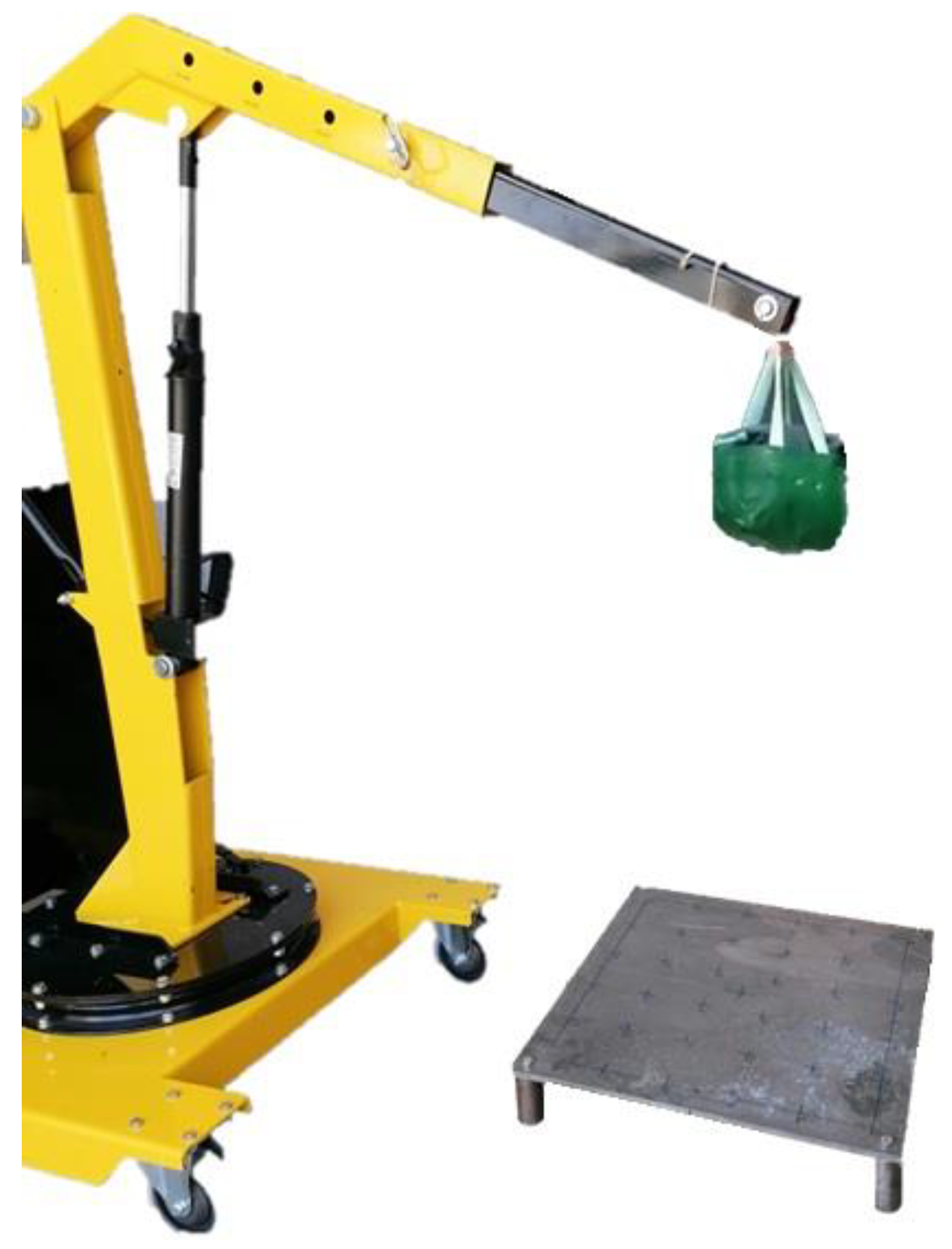
2. Experimental Set-Up and Numerical Simulations

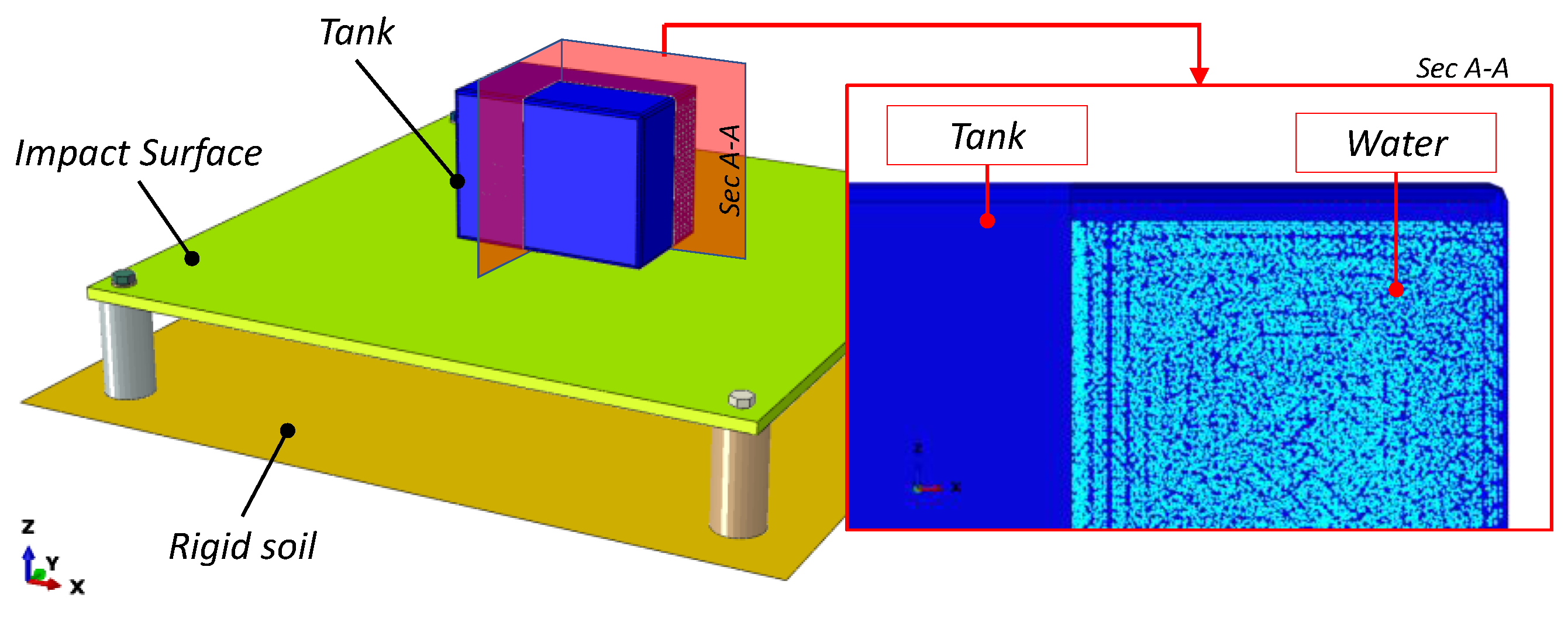
Experiments were carried out on a soft nylon bag filled with water and dropped from varying heights up to 2 m. The bag has a size of 210 × 130 × 160 mm³, and was filled with water balloons for a total weight of 4.1 kg. Two types of impacts were investigated: an impact hammer and a dropped object. The former was manually managed to generate random impacts. The latter allowed us to realize repeatable impacts of higher energy by dropping the object from a controlled height, thus enabling a more accurate control of the impact parameters.

The mass of the dropping object, along with the height of the drop, determine the energy of impact. Both influence the potential energy, as well as the resulting kinetic energy due to the drop. The nylon bag was dropped from four specific heights (0.5 m, 1 m, 1.5 m, and 2 m) to generate impacts with energies of 20.09, 40.18, 60.27, and 80.36 Joules.

In the drop impact test, a sensorised steel plate, equipped with four strain gauges, four piezoelectric (PZT) sensors and four fibre Bragg grating (FBG) sensors, was used to monitor the impact properties. The sensors were attached to the bottom side of the plate for measuring the bending strains. The set-up had no apparatus to measure the impact force directly. A PCB Piezotronics 086C03 hammer equipped with a load cell (sensitivity of 1.942 mV/N) to measure the impact force at the tip was used to generate impacts with random force. A soft rubber tip was selected to simulate the stiffness of the representative soft tank.

Unlike composites that can fail in a wide variety of modes and contain barely visible impact damage (BVID) [9], impact damage was not considered to be a threat to the selected metal plate, due to the large energy absorption capacity of the plate. The square plate of side 700 mm and thickness 12 mm was supported at the four corners. The drop test set-up is shown in Figure 1. The layout of the PZT, strain gauges, and FBG sensors is shown in Figure 2. Sensor positions were selected in order to balance two different needs: a good distribution of sensors with respect to the impact point, and a good correlation between different types of sensor data. The PZT sensors converting the lamb waves generated by the impact into voltage signals were recorded by a Siemens LMS SCADAS III acquisition system. Four strain gauges with gauge lengths of 5 mm were used to interpret the strain in a small area at specific locations. They were connected to the simultaneous bridge modules to form three wire quarter bridges. The sapling frequency was 5120 Hz per channel, on the condition that both PZT and strain gauges channels were acquired simultaneously. This fulfilled the requirement of measuring different sensor types and locations at the same time. Four FBG sensors, with a central wavelength of 1550 nm, were bonded on the plate near the strain gauges. The FBG sensors were mounted away from the edges of the plate, in order to have a maximum delay on the successive reflections of propagation wave, with no interference in the fundamental first part of the signal. The sensitivity and directionality tests were performed by a hammer test. All data processing was done in MathWorks MATLAB 2020b.

2.1. FE Model

The numerical model, developed in ABAQUS (2020 version, Dassault Systèmes Simulia Corp., Johnston, RI, USA) [10], consists of three main components: the plate (i.e., the impact surface), the bag (the impacting body), and the liquid contained in the bag (water).

The first one is made in an aluminium alloy, and therefore it is modelled by means of continuum solid elements and using the elasto-plastic material model (bilinear with isotropic hardening); the water was modelled by an SPH approach and the Hugoniot relationship; the bag was modelled with continuum shell elements and a hyperplastic material model. Such models are detailed in the following paragraphs.

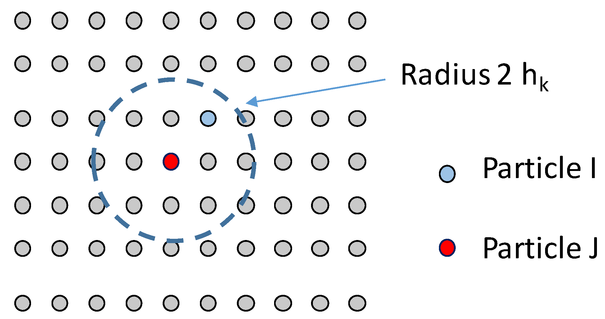
2.1.1. Water Modelling

The smoothed particle hydrodynamics (SPH) [11,12,13] are represented by three-dimensional elements with three degrees of freedom and defined by their centre of mass. These elements have their own shape functions that depend on the connectivity of the particles. The interpolation distance between the particles, called smoothing length, furnishes the location, and gives information about the transmission among the different particles.

In the SPH approach, the water is simulated as particles with the same dimensions and distances without mass. The velocity and energy of the particles at any time can be solved by means of a function f(x). The value of this function can be approximate for a datum particle, by Equation (1):

$$<f\left(x_i\right)>={\displaystyle \sum }_{j=1}^N\frac{m_j}{{\rho }_j}f\left(x_j\right)W\left(x_i-x_j,h\right)$$

(1)

where:

• h is the smoothing length
• m_i and ρ_i are the mass and density of the particle
• x_i and x_j are the position of the particles
• W is the kernel interpolation.

In particular, we consider two particles (i and j) as nearest neighbours, as shown in Figure 3. If the distance between the particle i and j is lower than the radius of the sphere of influence of j, i is connected to j. The dimension of the sphere of influence is a multiple of the particle’s smoothing length, and the multiplication factor depends on the kernel used to create the smooth particle’s shape function.

Therefore, the value of a variable for the particle J can be obtained by adding the contributions of the particle I contained in the influence radius. The interpolation kernel used in this paper is proposed by Monaghan [14].

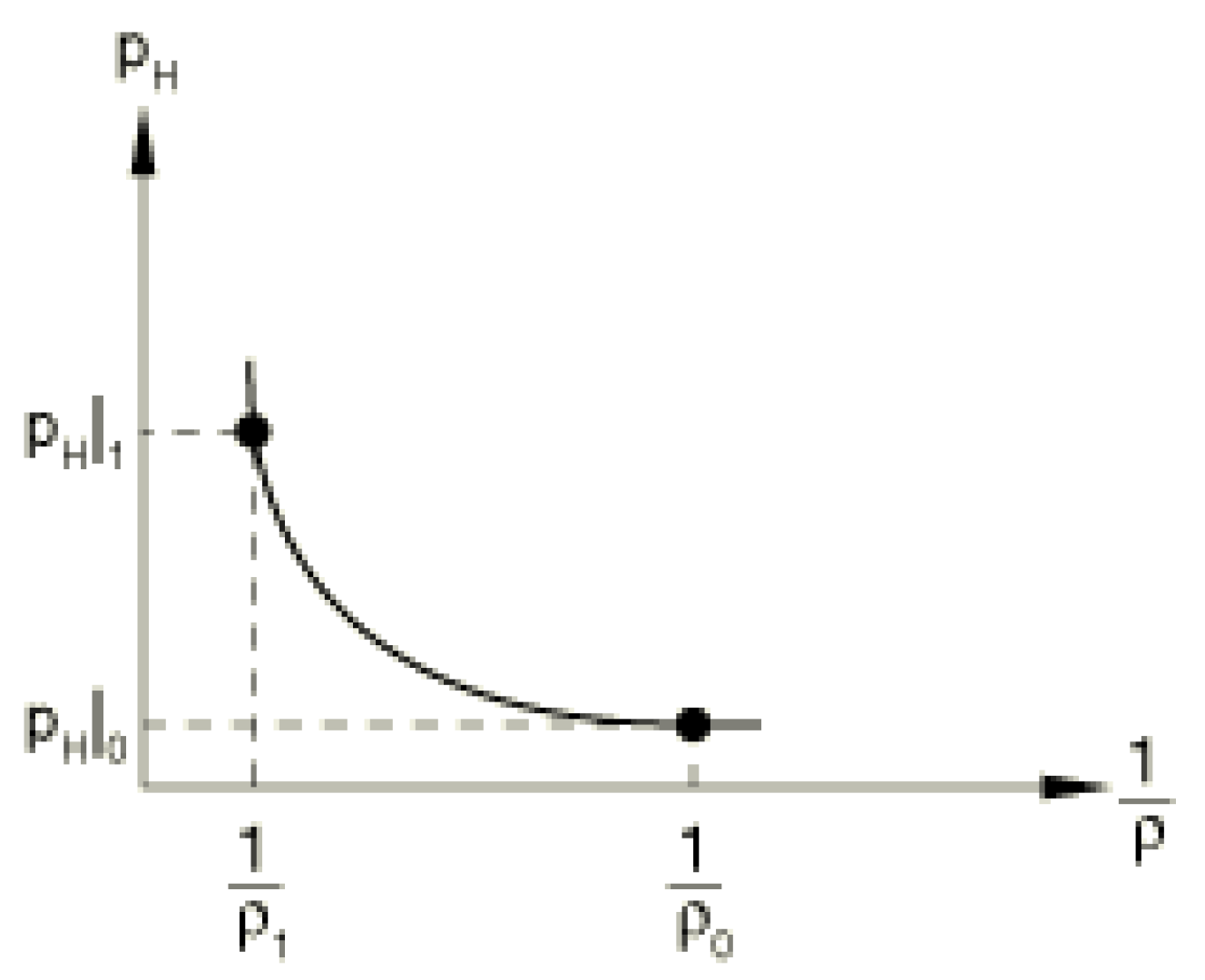
2.1.2. Water Material Model

The behaviour of the fluid material inside the fuel tank is regulated by the equation of state (EOS), relating pressure to a specific change rate of the material volume at a physical state.

The equation for the conservation of energy equates the increase in internal energy per unit mass, E_m, to the rate at which work is being done by the stresses, and the rate at which heat is being added. In the absence of heat conduction, the energy equation can be written as:

$$\rho \frac{\partial E_m}{\partial t}=\left(p-p_{bv}\right)\frac{1}{\rho }\frac{\partial \rho }{\partial t}+\mathrm{S} : \stackrel{·}{\mathrm{e}}+\rho \stackrel{·}{\mathrm{Q}}$$

(2)

where p is the pressure stress defined as a positive in compression, p_bv is the pressure stress due to the bulk viscosity, S is the deviatoric stress tensor, $\stackrel{·}{\mathrm{e}}$ is the deviatoric part of strain rate, and $\stackrel{·}{\mathrm{Q}}$ is the heat rate per unit mass.

The equation of state is assumed for the pressure as a function of the current density, ρ, and the internal energy per unit mass, E_m:

$$p=f\left(\rho , E_m\right)$$

(3)

which defines all the equilibrium states that can exist in a material. The internal energy can be eliminated from the above equation to obtain a p versus V relationship (where V is the current volume) or, equivalently, a p versus 1/ρ relationship that is unique to the material described by the equation of the state model. This unique relationship is called the Hugoniot curve, and is the locus of P-V states achievable behind a shock (Figure 4).

The Hugoniot pressure, p_H, is a function of density only, and can be defined, in general, from fitting experimental data. An equation of state is said to be linear in energy when it can be written in the form

$$p=f+g{E}_m$$

(4)

where f(ρ) and g(ρ) are functions of density only, and depend on the particular equation of the state model.

There are different formulations of EOS. The most common form, for water description, is the linear Us-Up equation, and is given by:

$$p_H=\frac{{\rho }_0{c}_0^2\eta }{{\left(1-s\eta \right)}^2}$$

(5)

where c₀ and s define the linear relationship between the shock velocity, U_s, and the particle velocity, U_p, as follows:

$$U_s=c_0+s{U}_p$$

(6)

With the above assumptions, the linear U_s −U_p Hugoniot form is written as:

$$p=\frac{{\rho }_0{c}_0^2\eta }{{\left(1-s\eta \right)}^2}\left(1-\frac{{\Gamma }_0\eta }{2}\right)+{\Gamma }_0{\rho }_0{E}_m$$

(7)

where ρ₀c₀² is equivalent to the elastic bulk modulus at small nominal strains.

There is a limiting compression given by the denominator of this form of the equation of state

$${\eta }_{lim}=\frac{1}{s}$$

(8)

or

$${\rho }_{lim}=\frac{s{\rho }_0}{s-1}$$

(9)

At this limit, there is a tensile minimum; thereafter, negative sound speeds are calculated for the material. The following parameters were used for the water material model: C₀ = 1.45 × 10⁶, s = 0; dynamic viscosity = 8.9 × 10⁻¹⁰; density = 1 kg/dm³.

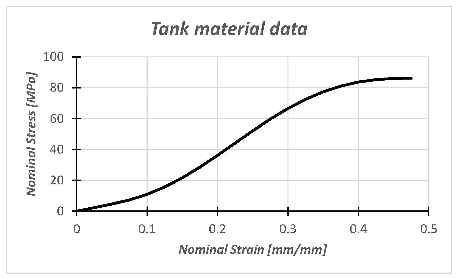
2.1.3. Tank Material Model

The fuel tank is composed of a standard nylon fabric textile. The adopted numerical material model is a hyperelastic material which is isotropic and nonlinear; and it is valid for materials that exhibit instantaneous elastic response up to large strains (such as rubber, solid propellant, or other elastomeric materials).

Hyperelastic materials are described in terms of a “strain energy potential,” U(ε), which defines the strain energy stored in the material per unit of reference volume (volume in the initial configuration), as a function of the strain at that point in the material. There are several forms of strain energy potentials available in Abaqus to model approximately incompressible isotropic elastomers: the Arruda–Boyce form, the Marlow form, the Mooney–Rivlin form, the neo-Hookean form, the Ogden form, the polynomial form, the reduced polynomial form, the Yeoh form, and the Van der Waals form.

For this material description, the Ogden form is used. A strain energy potential is constructed that will reproduce the test data exactly, and that will have reasonable behaviour in other deformation modes.

The form of the Ogden strain energy potential is:

$$U={\displaystyle \sum }_{i=1}^N\frac{2{\mu }_i}{{\alpha }_i^2}\left({\overline{\lambda }}_1^{ {\alpha }_i}+{\overline{\lambda }}_2^{ {\alpha }_i}+{\overline{\lambda }}_3^{ {\alpha }_i}-3\right)+{\displaystyle \sum }_{i=1}^N\frac{1}{D_i}{\left(J^{el}-1\right)}^{2i}$$

(10)

where λ_i are the deviatoric principal stretches and ${\overline{\lambda }}_i=J^{-\frac{1}{3}}{\lambda }_i$ are the principal stretches; N is a material parameter; and µ_i, α_i and D_i are temperature-dependent material parameters. The initial shear modulus and bulk modulus for the Ogden form are given by

$${\mu }_0={\displaystyle \sum }_{i=1}^N{\mu }_i; K_0=\frac{2}{D_1}$$

(11)

The particular material models described above—the Mooney–Rivlin and neo-Hookean forms—can also be obtained from the general Ogden strain energy potential for special choices of µ_i, α_i.

The nominal stress vs. nominal strain curve defining the hyperplastic behaviour of the tank is reported in Figure 5.

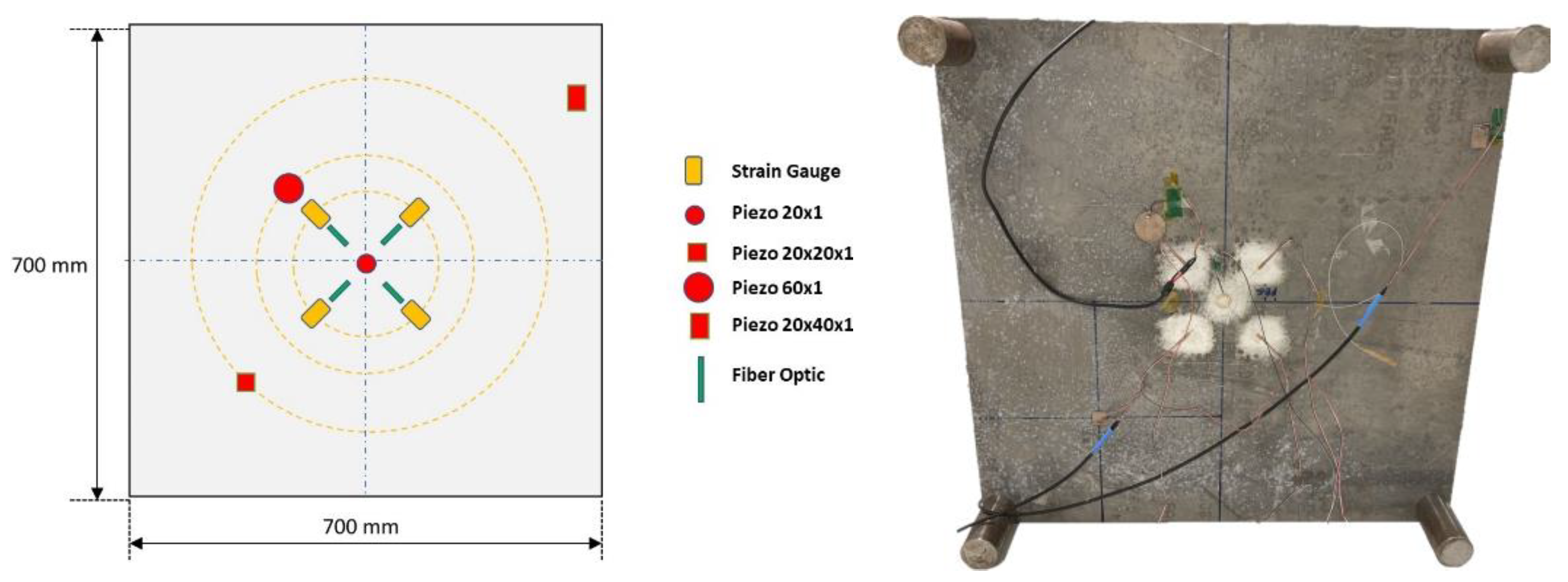
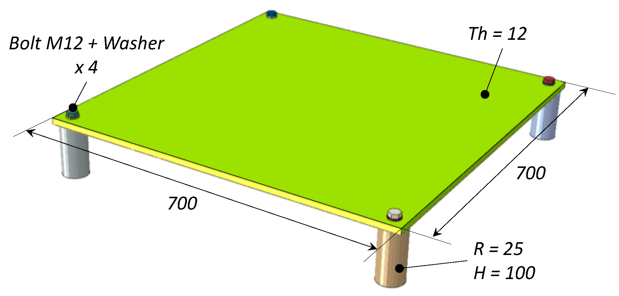
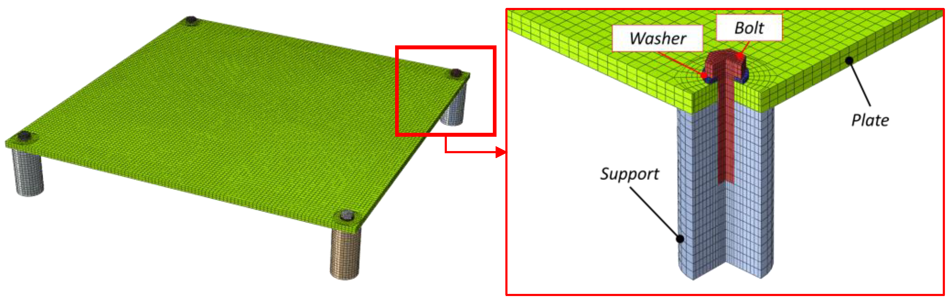
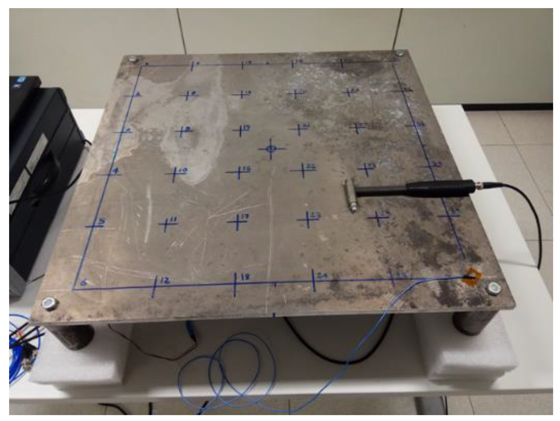
2.2. Instrumented Plate

The impact surface consists of an aluminium plate (Al 2024) and four aluminium cylindrical supports bolted together by means of 4 steel M12 bolts. The plate is 12 mm thick and 700 mm wide and long, while the supports radius is 25 mm, and their height is equal to 100 mm (Figure 6).

Both the plate and supports have been modelled by means of continuous 3D solid elements (Figure 7), and in particular, only hexahedral elements with a reduced integration scheme have been adopted (C3D8R). In total, the numerical model has 76,644 nodes and 59,564 elements (average in-plane mesh size equal to 7.5 mm). The same model was used both for the linear modal characterization and for the dynamic impact test, and therefore, in order to accurately evaluate the impact forces and the induced deformed shape, a fine mesh has been chosen.

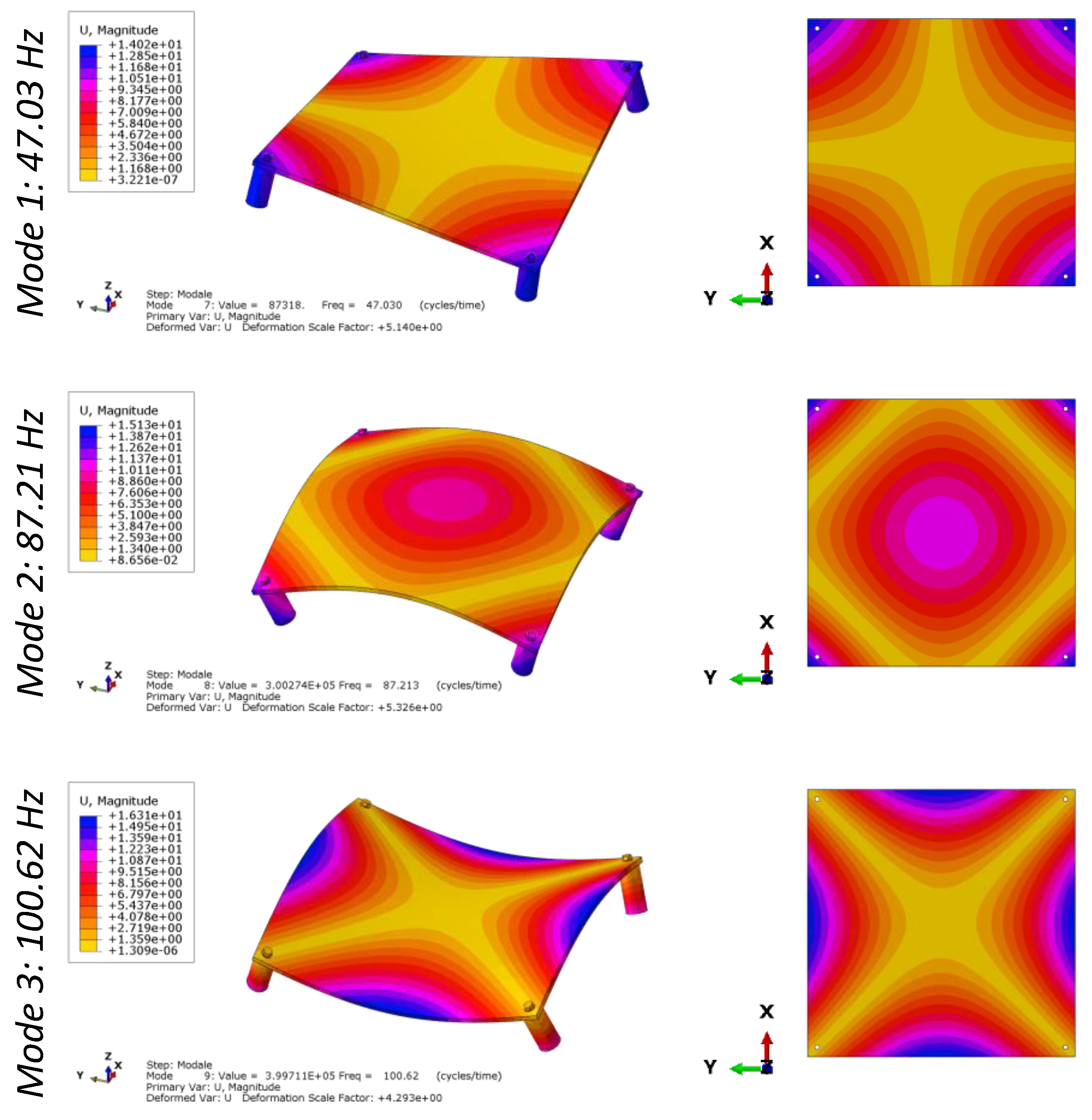
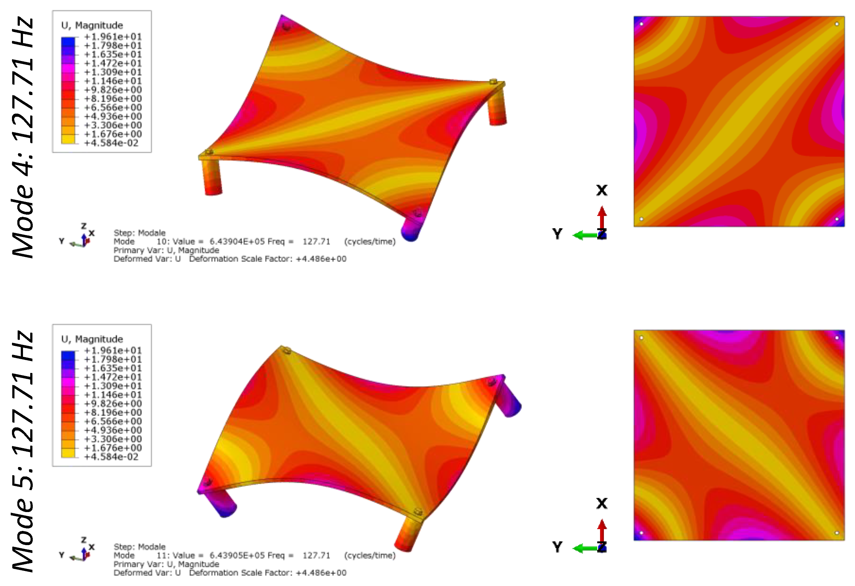
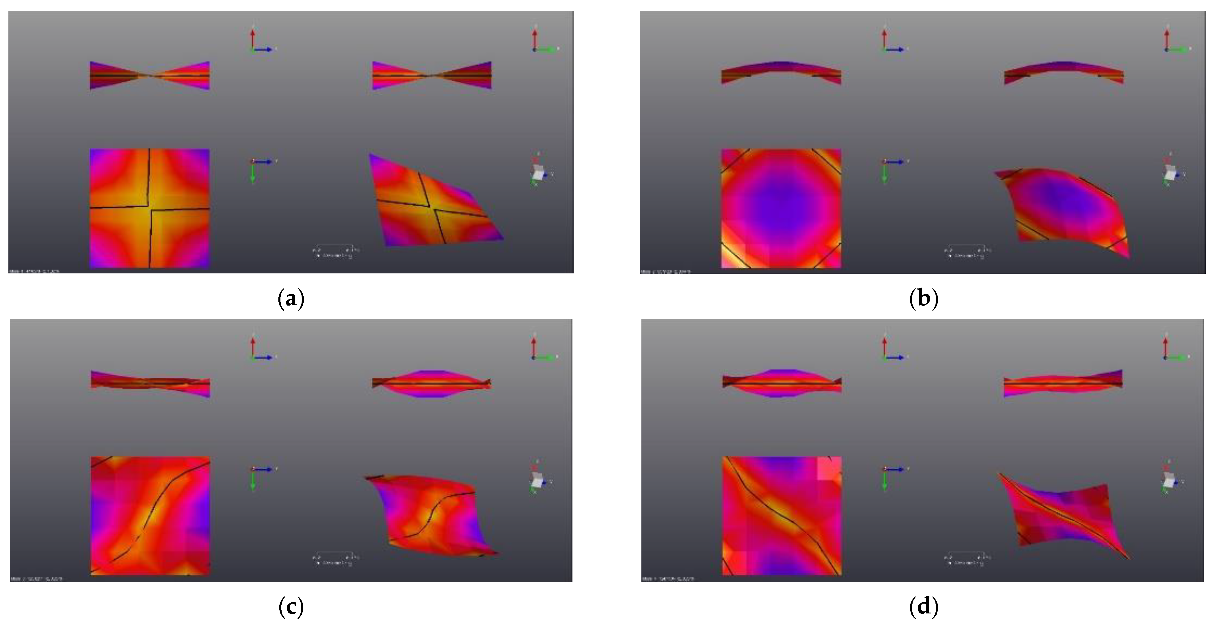
Numerical Modal Analysis

Modal analysis is a standard approach to estimate the dynamic modal parameters and validate the FE model against experimental modal data. By evaluating natural frequencies and modal shapes, it is possible to evaluate the global quality of the numerical model, since modal properties are affected by both the mass and stiffness distribution of the structure. When the structure is subjected to impact forces, it experiences a stress state concentrated in a very short time interval, which in turn triggers an oscillatory deformation field, depending on the dynamic response of the structure.

A numerical modal analysis was conducted under a free–free boundary condition, i.e., without the introduction of any constraints at the four angles. The modal analysis was carried out by means of Abaqus/standard code. The experimental test, as reported in the next section, was also performed in this condition. Results are listed in

Table 1. The numerical modal frequencies of the plate in free-free boundary conditions.

Mode Number	Free–Free Condition (Hz)
Mode 1	47.03
Mode 2	87.21
Mode 3	100.62
Mode 4	127.71
Mode 5	127.71

.

Figure 8 shows the modal deformation of the first 5 modes taken into consideration (since the simulation has been performed in the free–free condition, the first six modes correspond to rigid translations and rotations, and therefore the first mode to be considered is the 7th mode). The first mode can be classified as a torsional mode. The second and third instead represent bending modes (according to the in-plane X and Y axes). The fourth and fifth modes are bending-torsional modes.

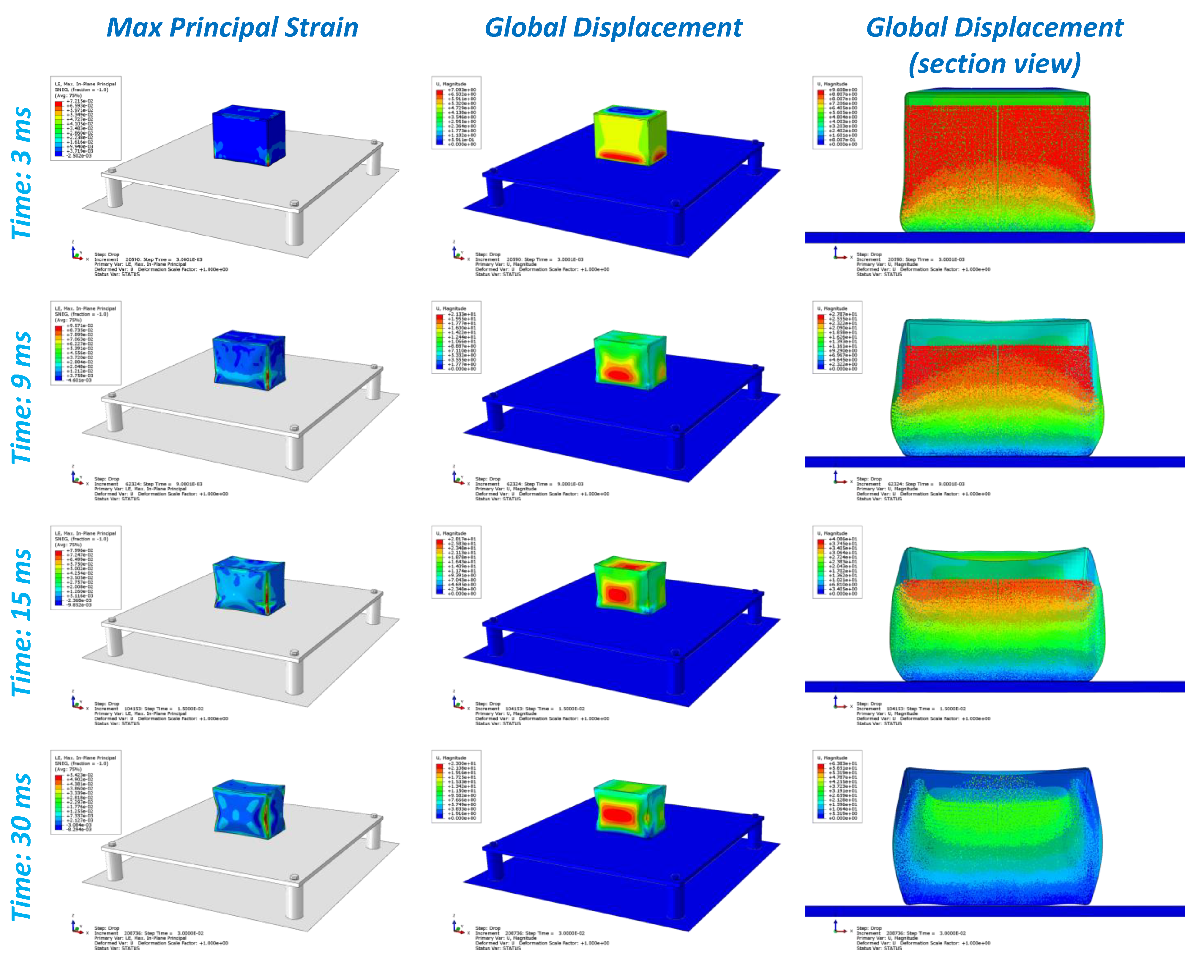
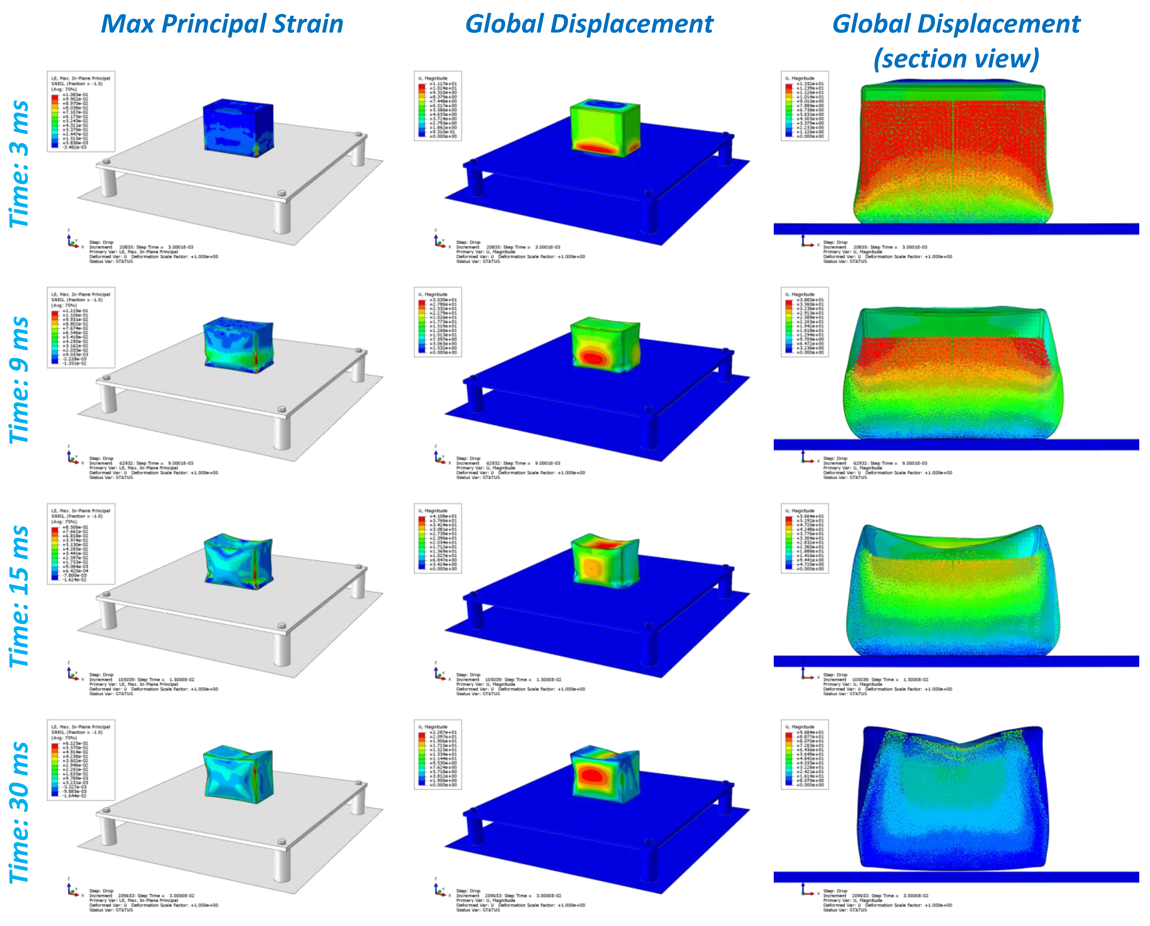
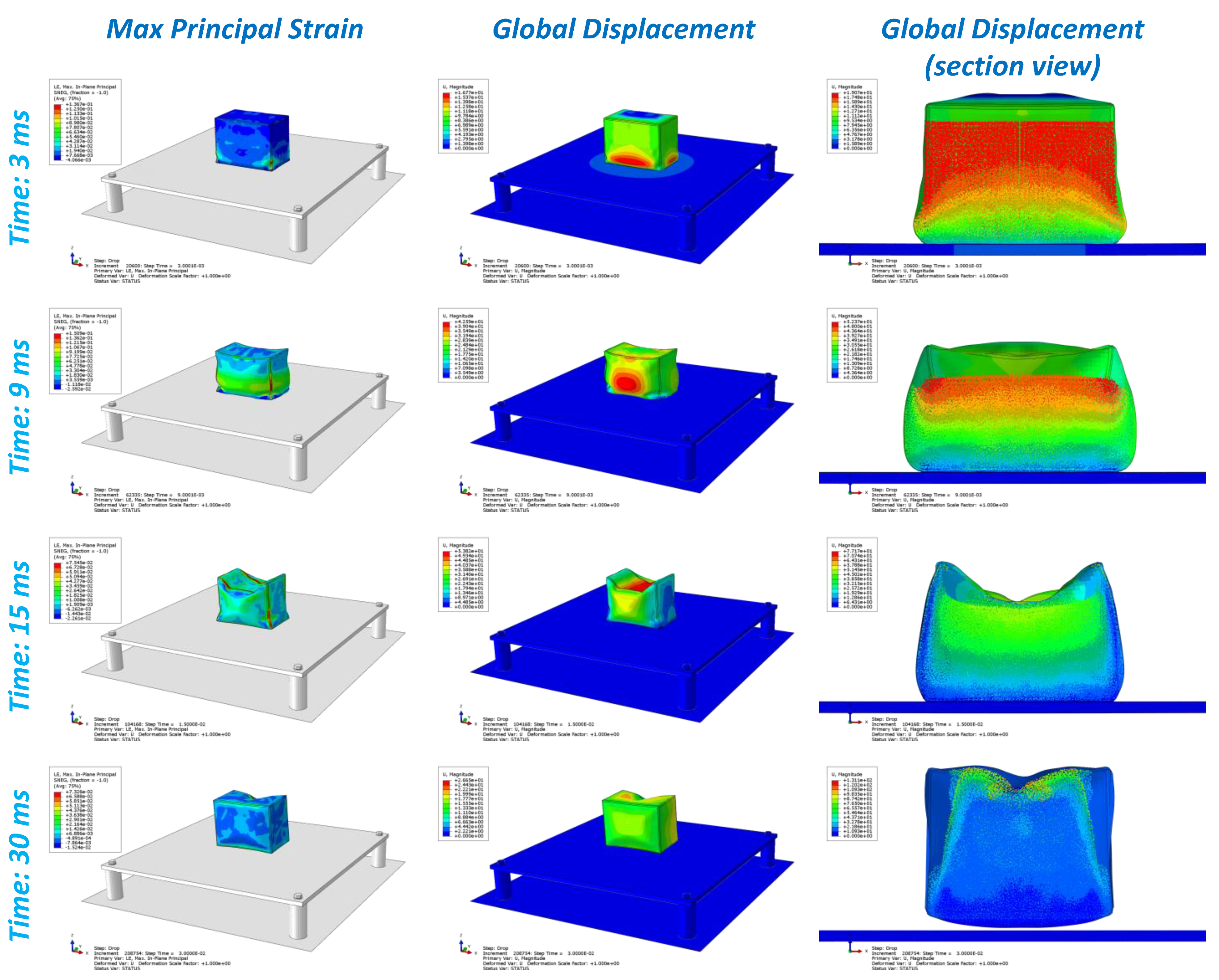
2.3. Drop Test Simulations

To evaluate the deformation state induced on the plate, three different drop tests (and thus impact energies) were simulated from three drop height values: 0.5 m, 1.0 m, and 2.0 m. A dynamic impact simulation was performed by means of Abaqus/explicit code.

In all cases, the tank mass, including the liquid (water) inside, is equal to 4.1 kg. The tank is 210 mm long, 130 mm wide, and 160 mm high, and is made of a commercial nylon fabric. Therefore, considering that the empty tank weighs about 200 g, the filling percentage is about 90%.

In order to avoid over-constraints, the soil was modelled as a rigid surface, and a friction contact was defined between the soil and the supports of the impact plate. In order to reduce the computation costs, the tank was positioned at a reduced distance from the impact surface, and a suitable impact velocity was applied to it (converting potential energy into kinetic energy). Therefore, the impact speeds are 3.13 m/s, 4.43 m/s, and 6.26 m/s, respectively. Figure 9 shows the model with the detail of the inner water modelled by SPH.

The results of the drop test simulations are reported in Figure 10, Figure 11 and Figure 12, in terms of global displacement for the entire model and in section view, where it is possible to appreciate the inner sloshing. The water is subject to considerable sloshing that generates a new mass distribution with respect to the initial state and it induces a deformation state on the tank that reaches about 9%, 12% and 16% for the drop heights equal to 0.5 m, 1 m and 2 m, respectively. The flexible tank did not exhibit any damage likely to cause the fluid leakage of liquid after the impacts.

Figure 13 shows the time history of the strain components evaluated on the lower surface of the impacted plate (opposite side with respect to the impact). The components ε₁₁ and ε₂₂ correspond to the strain components along the x and y axes of the global reference system (the elements of the plate are aligned with the global reference system).

The general behaviour of the three tests is very similar. There is a first peak immediately after the contact, which obviously depends on the two elastic bodies. The second peak, the highest one, occurs after about 5 ms. After this instance, the particles that have impacted the lower surface of the tank (inner side) start to rebound against the other particles that are coming, and therefore slow down their run. This is the main reason why a fall in deformation curves can be appreciated immediately at this instant. Similar behaviour was recorded for all cases, but obviously, the times are slightly different. The sloshing effects play a fundamental role in this type of test; in fact, due to the sloshing motion, the particles are continuously redistributed in the volume, generating oscillations in the pressure field induced on the plate, which then generate oscillations in the deformation state.

It is worth noting that the moment of maximum deformation, detected on the plate, does not correspond to the instance of a maximum tank crushing in any of the analysed cases. Figure 14 also shows the best polynomial functions that fit the peak values of strains predicted on the plate due to the variable height impacts.

The displacement in the z direction of the central point of the upper face of the tank is shown in Figure 15. As the impact speed increases, the maximum displacement increases (in absolute value) and occurs earlier in time.

3. Signal Deconvolution

One of the major challenges faced in impact engineering is that of reconstructing the history of impact force when it is difficult or impossible to be measured directly. The deconvolution method was proposed by Inoue et al. [15,16] for identifying an impact force history in a time domain from strain responses. The validity of this method was verified by experimental transfer functions between impact forces and strain responses, for the cases with given force locations in advance. Wu et al. [17] used Green’s functions with the eigenmode expansion method to identify impact force histories, by minimising the residual error between experimental and numerical strain responses. N. Hu [18] used a Chebyshev polynomial to model a low-velocity impact force history, acting on a CFRP laminated plate equipped with four embedded piezoelectric sensors, by solving the inverse problem through the quadratic programming optimum method. Seno et al. [19] have recently proposed a novel gradient method to estimate the maximum impact force of low energy non-damaging impacts under varying operational and environmental conditions. A linear relationship was also found between the maximum absolute signal amplitude given by PZT sensors and the maximum impact force. These results expand on previous linear relationships between impact severity (energy or force) and impact signal features (energy, amplitude), proven by previous studies [20,21,22].

Indirect methods, such as signal deconvolution, use the output responses (caused by the unknown impact force), such as acceleration, displacement, strain, etc. to reconstruct the profile of an unknown impact force once the impulse response function is known. The response measured on the structure is thus expressed by the convolution of the input signal with the system’s impulse response. If the points of input and measurement are known, then

$$y_m\left(t\right)=h_y\left(t\right)\ast f\left(t\right)={{\displaystyle \int }}_{-\infty }^{\infty }{h}_y\left(t-\tau \right)f\left(\tau \right)d\tau$$

(12)

For strain measurements, Equation (1) becomes

$${\epsilon }_m\left(t\right)=h_{\epsilon }\left(t\right)\ast f\left(t\right)$$

(13)

where the subscript m means the measured value.

In the Fourier domain, the convolution that gives the output of the system can be transformed to a multiplication of the spectral components of the impulse response and the original input.

The deconvolution method is thus able to give an estimate of the unknown force f(t). The transfer function, which is the inverse of the spectral convolution, may be numerically estimated or obtained experimentally by measuring the force profile and the resulting response of the impact at each location. If the transfer function is known, one can rebuild the original impact signal profile from the measured strain signals through the multiplication of the spectral components of the response with the measured transfer function, followed by an inverse Fourier transform. However, since the problem is ill-posed, a regularisation procedure is often required to restrict the space of admissible unknowns and recover some kind of stability.

4. Experimental Results

As specifically, concerns load and damage monitoring, strain gauges and piezoelectric sensors are well-known devices that have already proven a range of practical applications. Due to deformation, the electric resistance of strain gauges, measured with a Wheatstone bridge circuit, changes proportionally to the applied force. This can be used with very high precision to calculate static, quasi-static tensile, and compression forces. On the other hand, piezoelectric technology is better suited to the measurement of dynamic force, which is the electric output signal related to the mechanical force through the intrinsic characteristics of piezoelectric materials. Furthermore, fibre optic sensors have shown potential for the continuous real-time monitoring of operating structures.

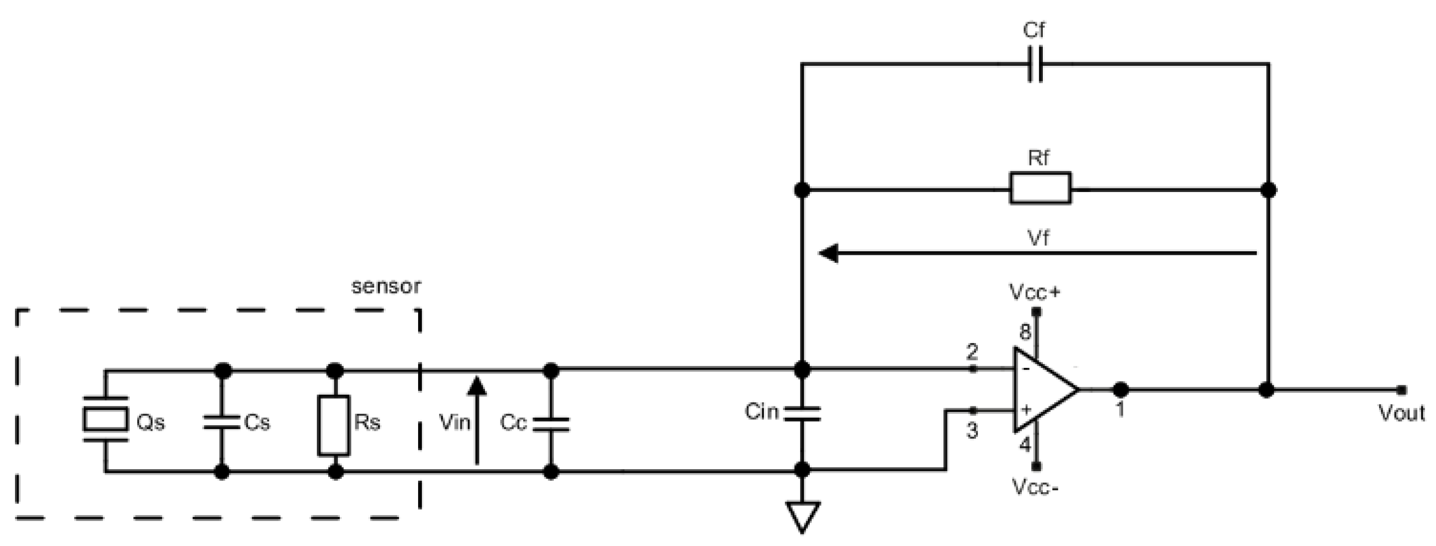
4.1. Electronic Circuit for Impact Measurements with PZT Sensors

When using thin circular PZT as strain sensors bonded on the structure, the output voltage V_PZT is proportional to the summation of in-plane strains as follows:

$$V_{PZT}\left(t\right)=G_{PZT}\left\{{\epsilon }_x\left(t\right)+{\epsilon }_y\left(t\right)\right\}$$

(14)

where G_PZT is the sensitivity of the PZT sensors which is calibrated using strain gauges during the impact test.

The charge produced by a piezoelectric material in response to the mechanical strain is typically quite small. In order to convert the charge generated by the piezoelectric sensors into readable signals for the data acquisition system, a dedicated charge amplifier was designed. An electronic circuit was thus created for signal conditioning their output.

The following parameters were considered for the piezoelectric sensors:

−

piezoelectric coefficient d31 = 280 × 10^–12 C/N

−

static capacitance (Cs) = 9 nF.

The maximum input voltage accepted by the data acquisition system was ±10 V. The electronic circuit is illustrated in Figure 16.

where:

• Qs is the input charge
• Cs and Rs are the characteristic parameters of piezoelectric
• Cc is the cable capacitance
• Cin is the amplifier input capacitance
• Cf is the feedback capacitance
• Rf is the feedback resistance

When the input charge, Qs, is applied to the inverting input of the amplifier, it is distributed among the cable capacitance, Cc, the amplifier input capacitance, Cin, and the feedback capacitor, Cf, as follows.

$$Qs=Q{C}_c+Q{C}_{in}+Q{C}_f$$

(15)

By considering Q = CV, we can write:

$$Qs=V_{in}\left(C_c+C_{in}\right)+V_f{C}_f$$

(16)

where V_in is the differential voltage of the op amp and V_f is the voltage in the feedback loop.

Due to the large gain of the op amp (AVD), the same potential tends to exist between pin+ and pin−. Consequently, we can consider that V_in = 0 and simplify Equation (16) as follows:

$$Q_s=V_f·C_f$$

(17)

As V_out = −V_f:

$$V_{out}=-\frac{Q_s}{C_f}$$

(18)

Looking in more detail at the closed-loop transfer function, we have:

$$V_{out}=-\frac{ jw ·Q_s·R_f}{1+jw·R_f{C}_f}$$

(19)

We can see that the Rf resistor must be as high as possible to keep the pole low.

Based on these considerations, an electronic board was designed and realized for each piezoelectric channel of the set-up. It is shown in Figure 17. In order to have greater flexibility in regulating the gain of the charge amplifier C_f, three capacitors were applied in parallel, and can be connected and disconnected independently. The optimal configuration was found by using two capacitances of 220 nF and one capacitance of 330 nF. To mitigate the pole effect, Rf was set to 1.5 kΩ, which put the pole at about 137 Hz. The voltage attenuation was estimated to be about −41 dB.

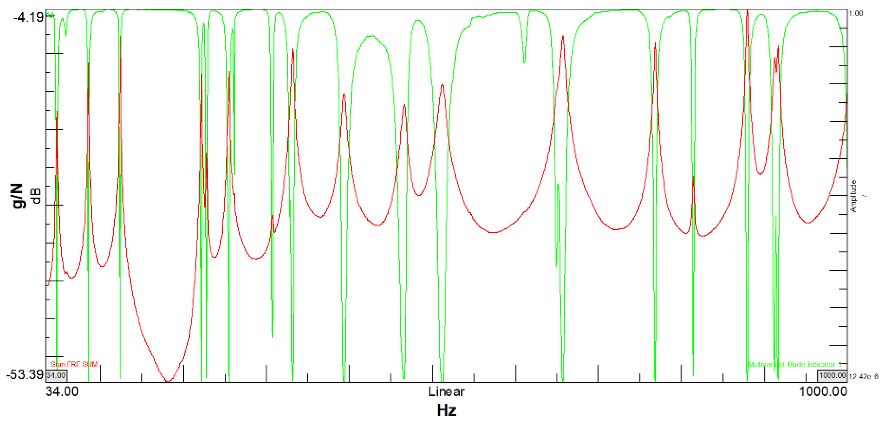
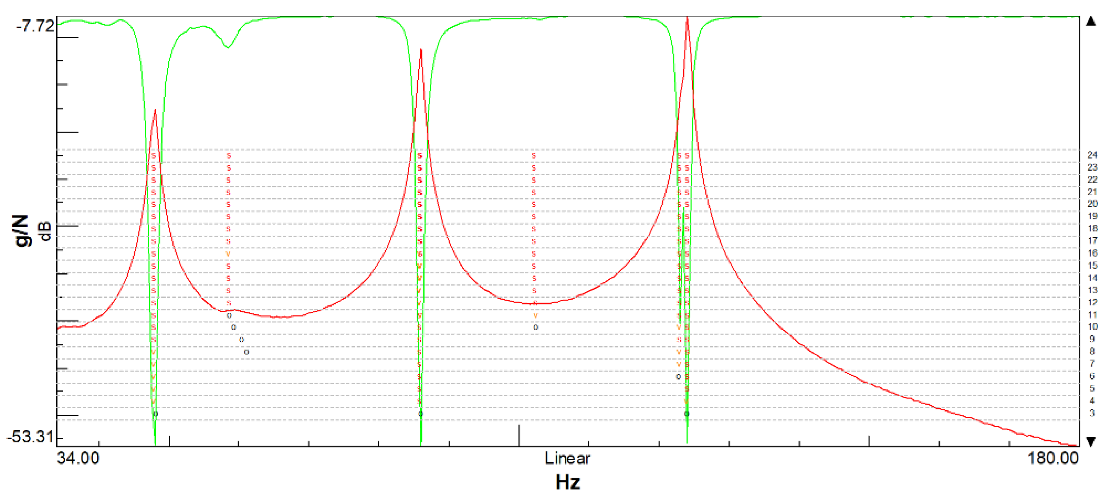
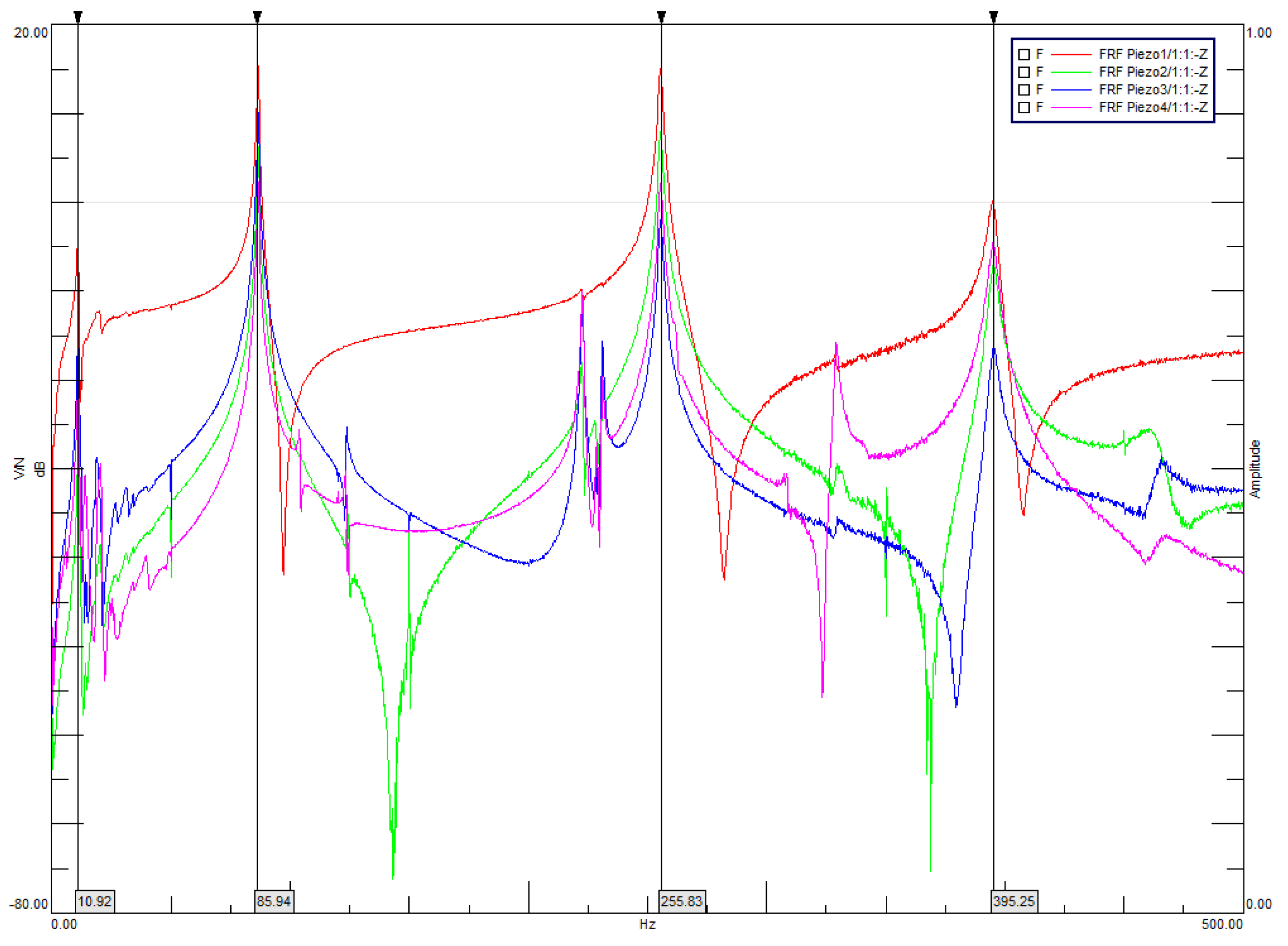
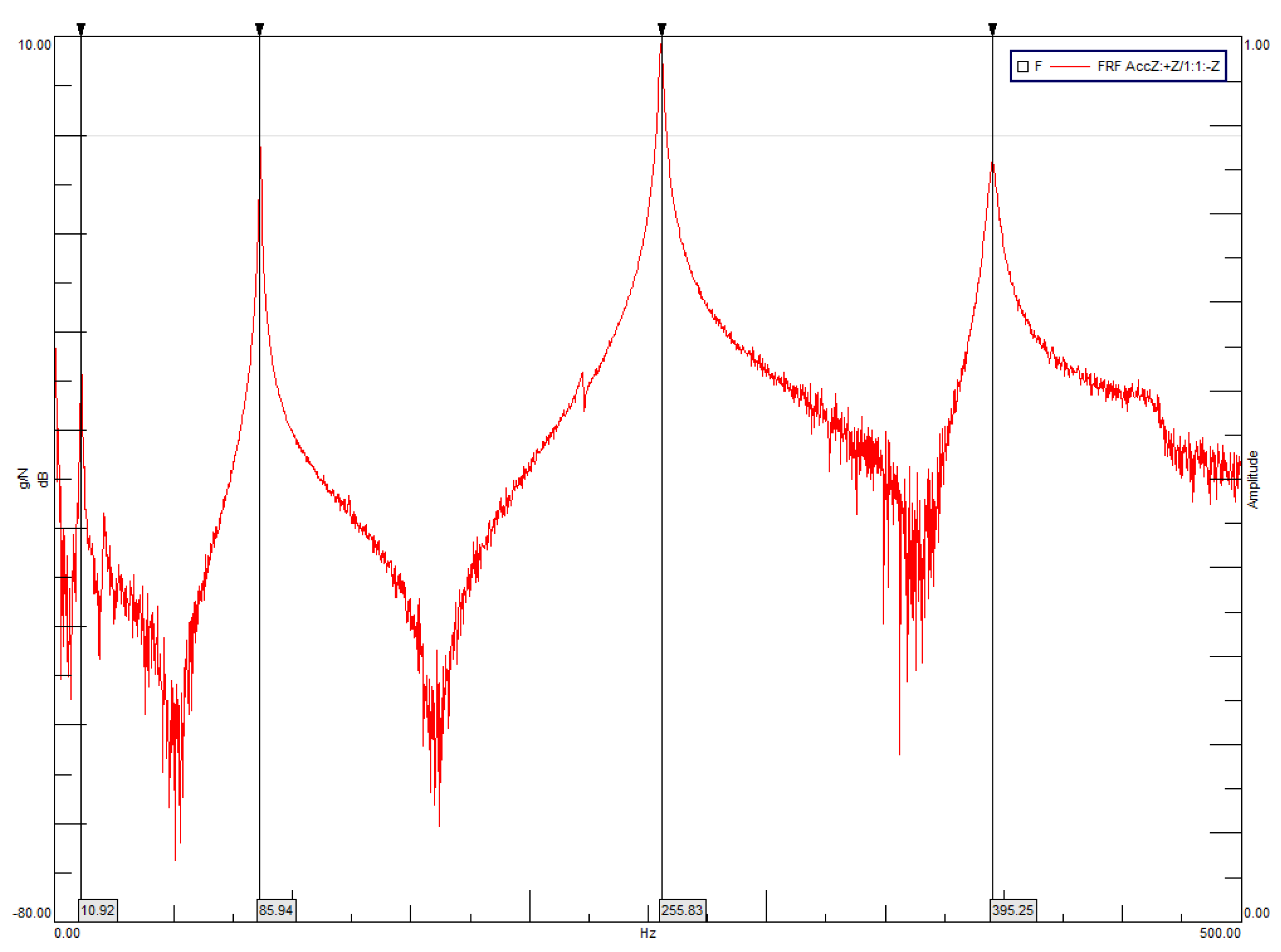
4.2. Experimental Modal Analysis

In order to characterize the dynamic behaviour of the impacted plate, a modal test was performed using the impact hammer, Figure 18. The plate was placed on a very soft foam base to simulate free–free boundary conditions. A grid made of 37 nodes was drawn on the plate (6 nodes along X times, 6 nodes along Y, plus one central node). Only one accelerometer was placed on edge node 36. The sensor was a PCB 356A01 accelerometer with a sensitivity of 0.481 mV/m/s².

The structure was globally simple from a dynamic point of view. Only the first few modes were extracted within a frequency range up to 1024 Hz. Such modal frequencies and shapes were sufficient to update the numerical model and make it suitable for drop test analyses.

The sum of the acquired FRF and the MIF is shown in Figure 19. A mode is typically expected where the SUM of FRF has a peak and the MIF drops to 0.

The modes were identified using the Polymax algorithm implemented in Siemens LMS software. The modes extracted in the range 30–180 Hz are reported in Figure 20.

Four modes were identified at the following frequencies: 47.9 Hz, 85.9 Hz, 123.0 Hz, and 124.1 Hz, showing a damping factor lower than 1%. The last two modes have very close natural frequencies because of the structural symmetry. On the contrary, the first two modes do not have their symmetrical counterparts, so they do not appear in a couple. The first four experimental modes are reported in Figure 21.

Numerical—Experimental Modal Correlation

A comparison of the numerical and experimental modes of the plate is reported in

Table 2. The comparison between numerical and experimental modal frequencies of the plate.

Mode Number	Numerical (Hz)	Experimental (Hz)	Error (%)
Mode 1	47.03	47.84	−1.7%
Mode 2	87.21	85.90	1.5%
Mode 3	100.62	-	N.A.
Mode 4	127.71	123.01	3.8%
Mode 5	127.71	124.10	2.9%

. The numerical results are in good agreement with the experimental data, showing a maximum error of 3.8%. Only the third mode at about 100 Hz was not experimentally identified by the single accelerometer, since it was located near the nodal line for this mode.

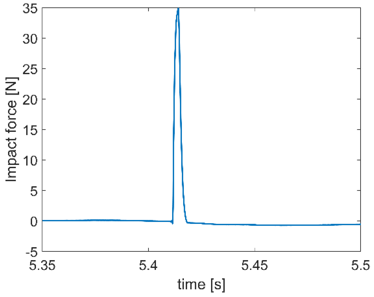
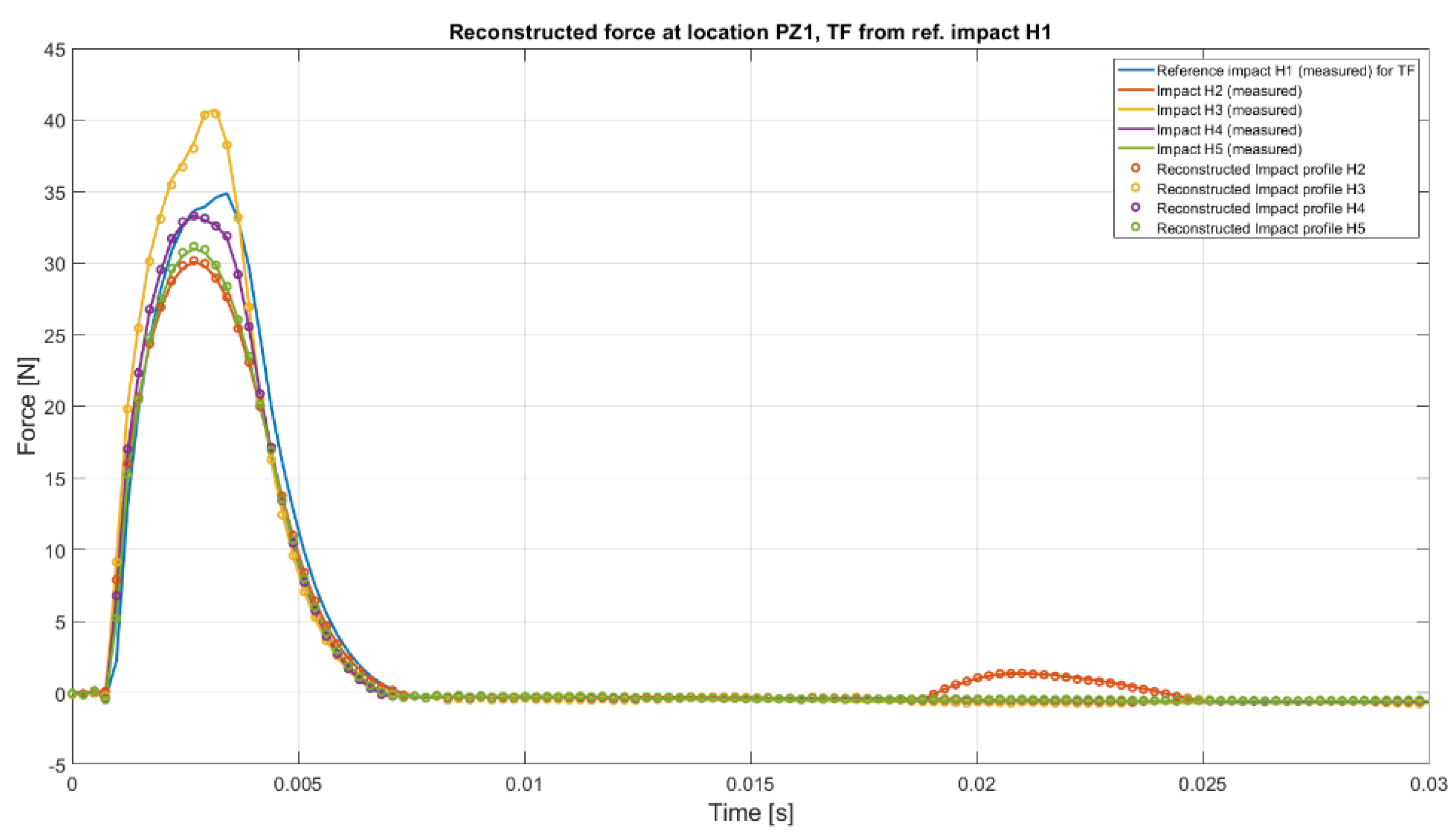
4.3. Reconstruction of Impact Force Profiles

The deconvolution method was then implemented to reconstruct the impact force profiles generated by an impact hammer in the previously described setup [23,24,25]. The output response is measured by both the piezoelectric sensors and the accelerometer.

The impulse signal generated by the impact hammer was the reference transient load used for preliminary assessments. Given that for a linear system, a linear relationship occurs between impact forces and impact signal response amplitudes, we used this method to evaluate if the whole impact force profile could be estimated with a good level of accuracy by using the transfer function obtained from a set of known impact cases, characterised by smooth peaks and a long contact time.

Typically, the response of a linear, time-invariant system to transient loading comprises two parts: the homogeneous solution and the particular solution. Due to the hit of a hammer, the forced motion takes place when the short duration impact load excites the structure, causing it to undergo forced vibration (the particular response). When there is no more load, the structure is free to vibrate at the natural frequencies (the natural response) until the kinetic energy is dissipated through damping. In order to observe the characteristics of an impact response, both the force profile generated by the hammer and the resulting piezo signal acquired at the centre of the plate are shown in Figure 22 and Figure 23, respectively. It is worth noting that, during the impact, the measured signal has a sharp peak in the vicinity of the impact site, and then the resulting strain propagates through the plate. It can also be seen that the response is proportional to a weighted average of the input function. After the impact, the structure starts to freely vibrate, and it experiences an amplitude decay due to the damping.

Plotting the particular response amplitude vs. the maximum impact force (Figure 24), we can see the recorded signals from both the piezoelectric sensors and the accelerometer scale linearly with the impact force magnitudes irrespective of the input force profile.

Figure 25 and Figure 26 show the experimental FRFs recorded by four piezoelectric sensors and the single accelerometer placed on the plate, respectively. As in other studies [26], it is shown that the values of the natural frequencies can be properly estimated by using PZTs. However, it is worth noting that only mode 2 can be clearly identified evaluating the FRFs’ peaks, since both the piezoelectric sensors and the accelerometer were in nodal positions for modes 1, 4, and 5 of vibration.

As there were four piezoelectric sensors on the plate, we obtained a reference transfer function for each piezo sensor, and reconstructed the impact force profile individually. The results are shown in Figure 27. It can be seen that the reconstructed impact forces match the experimental ones very well, although they were measured by strain sensors mounted on the plate.

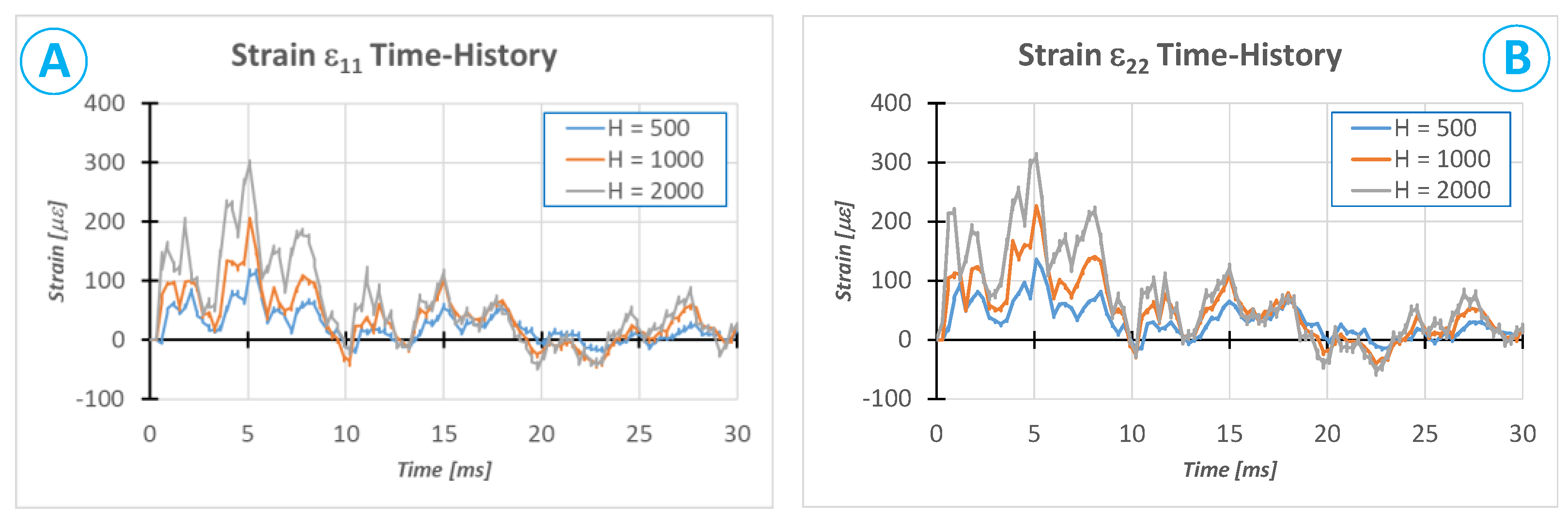
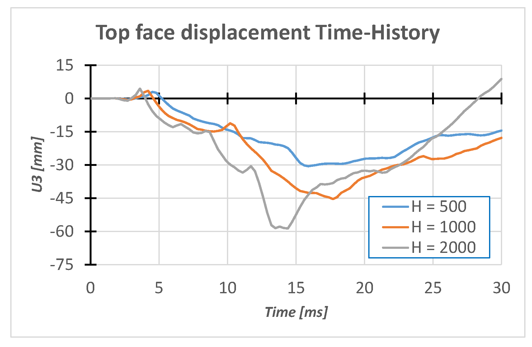
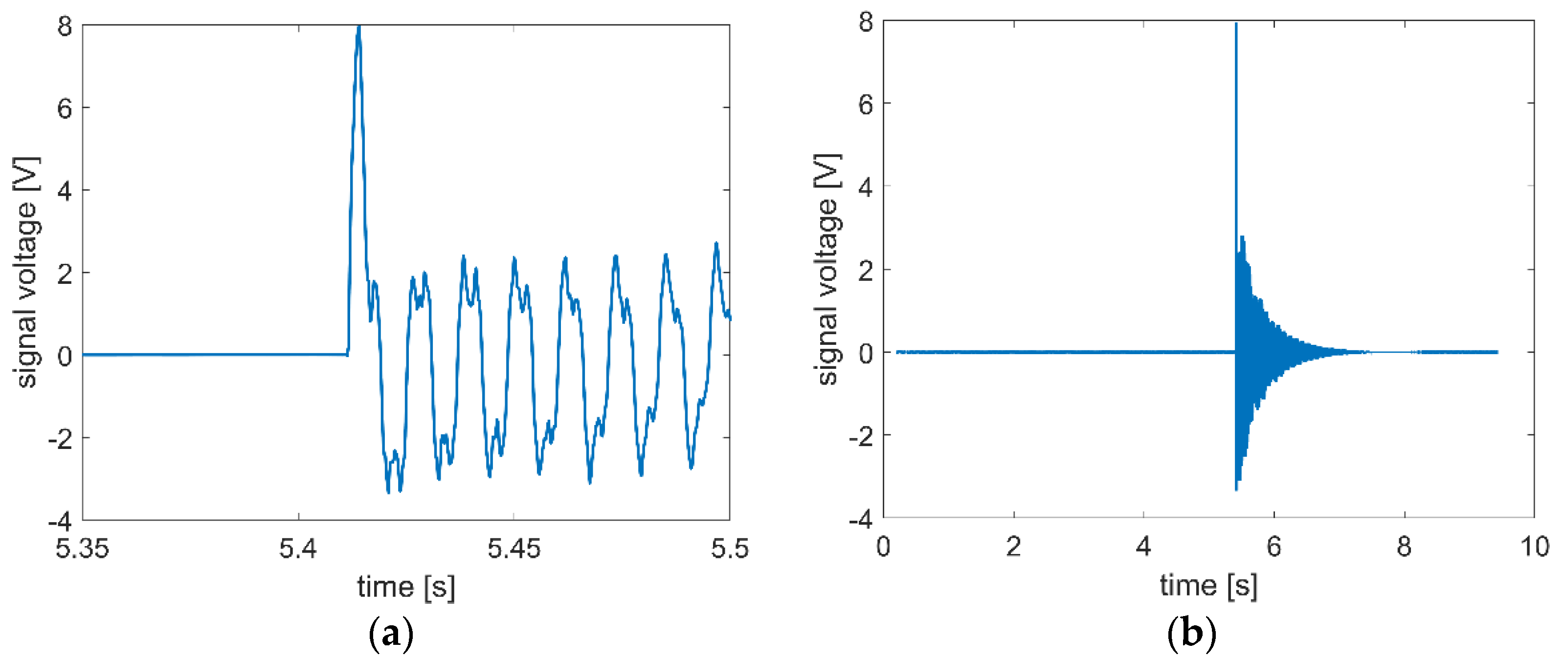
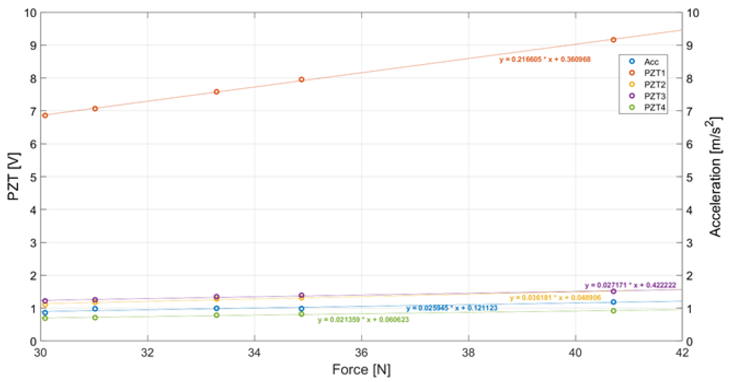
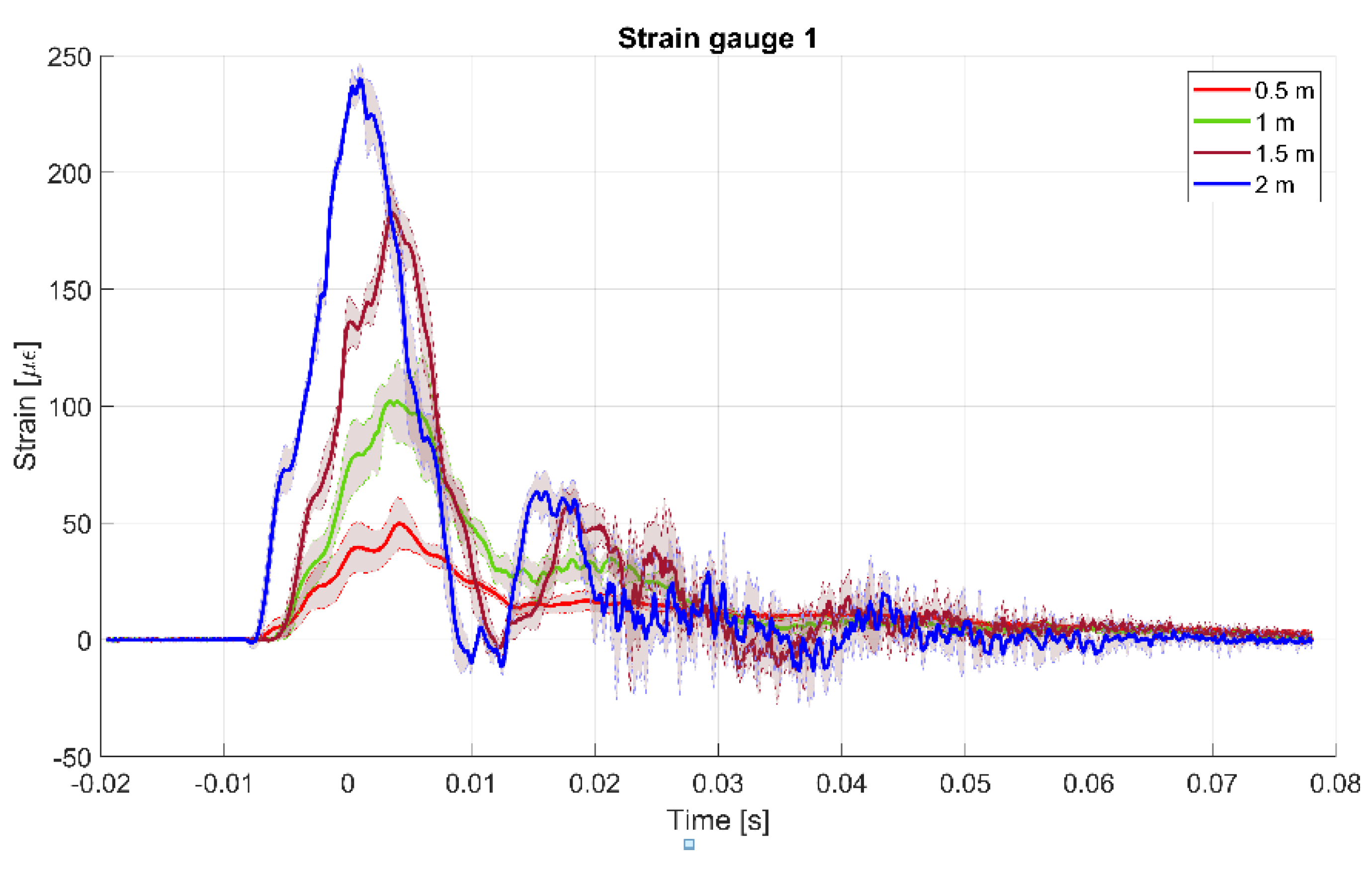
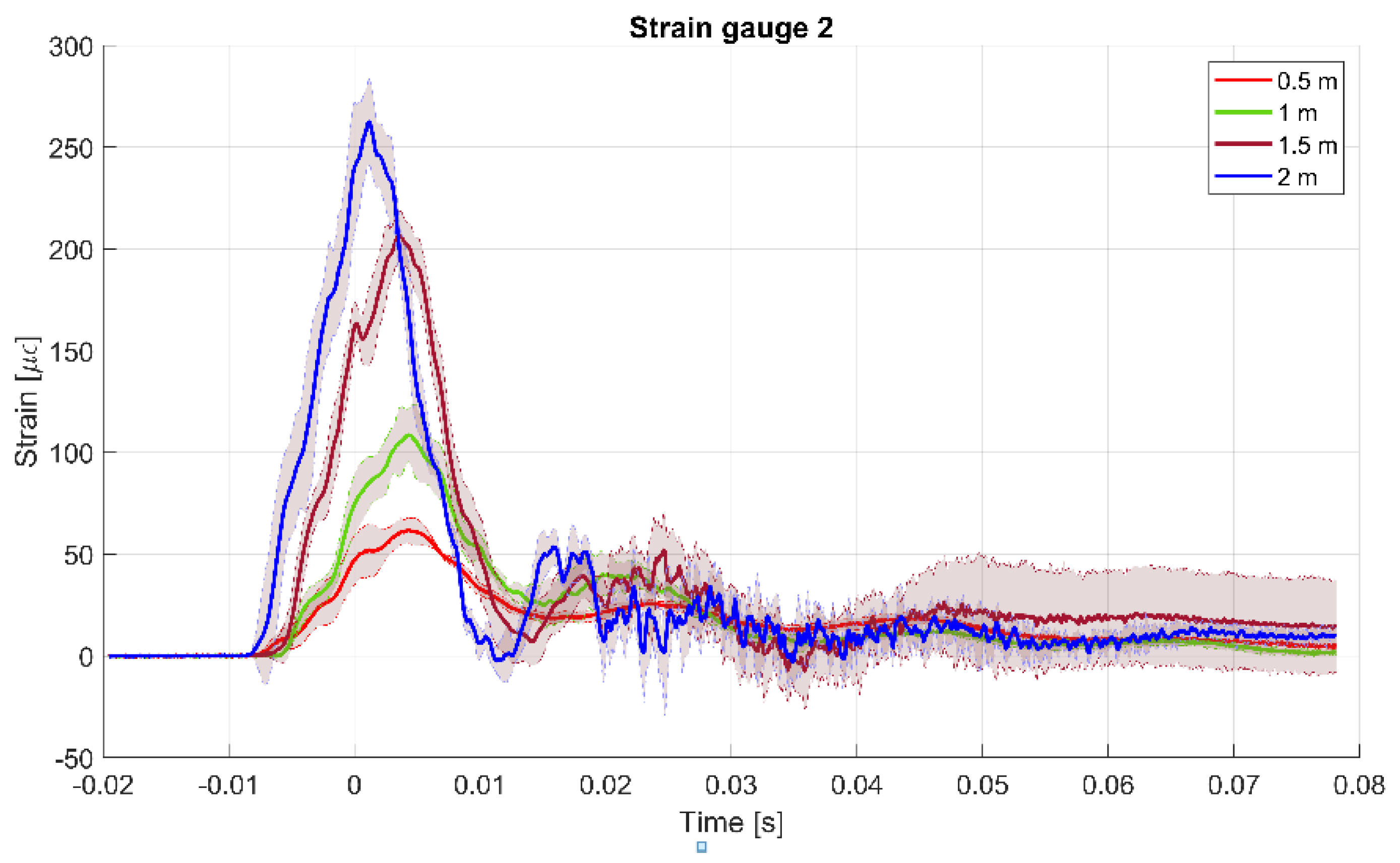
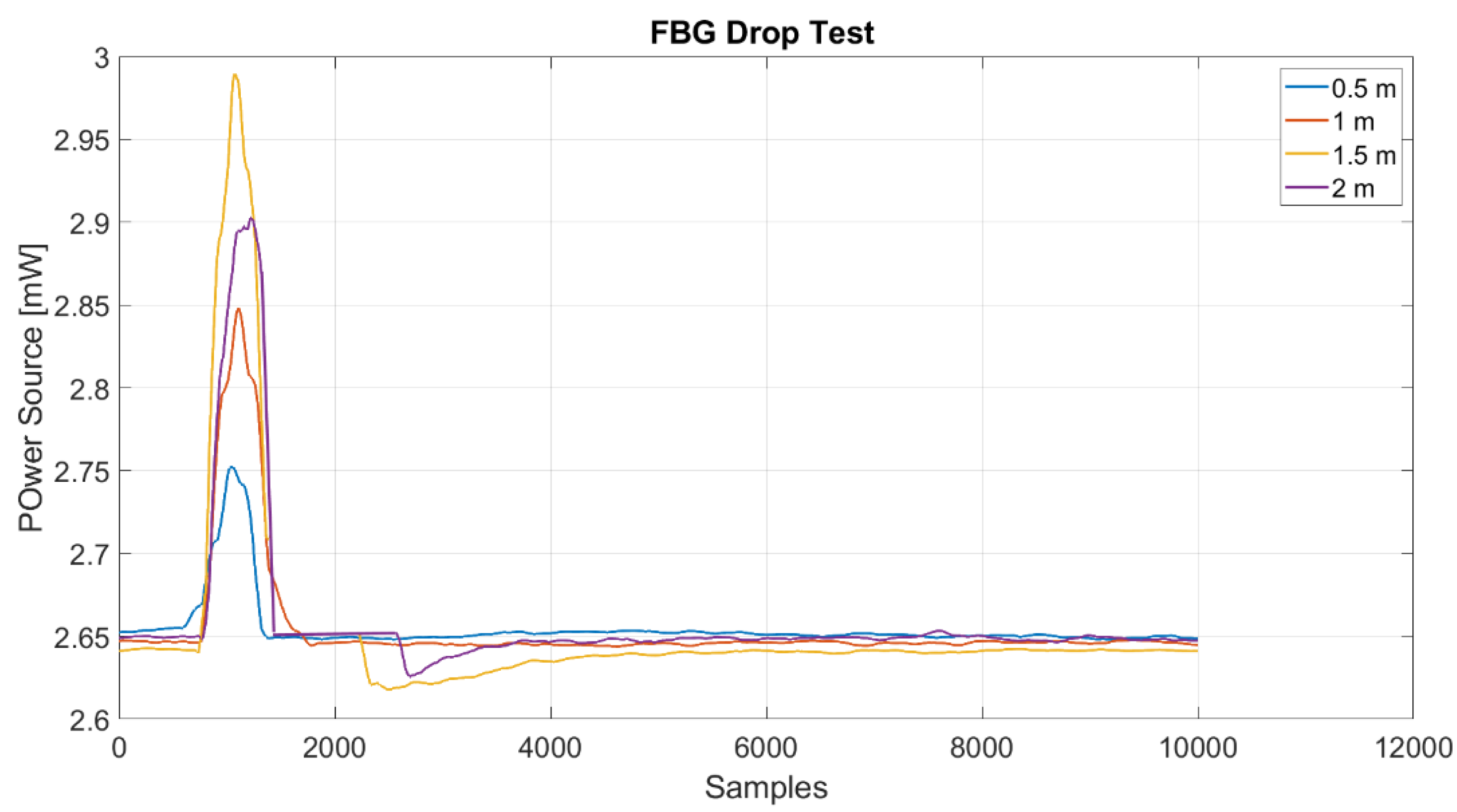
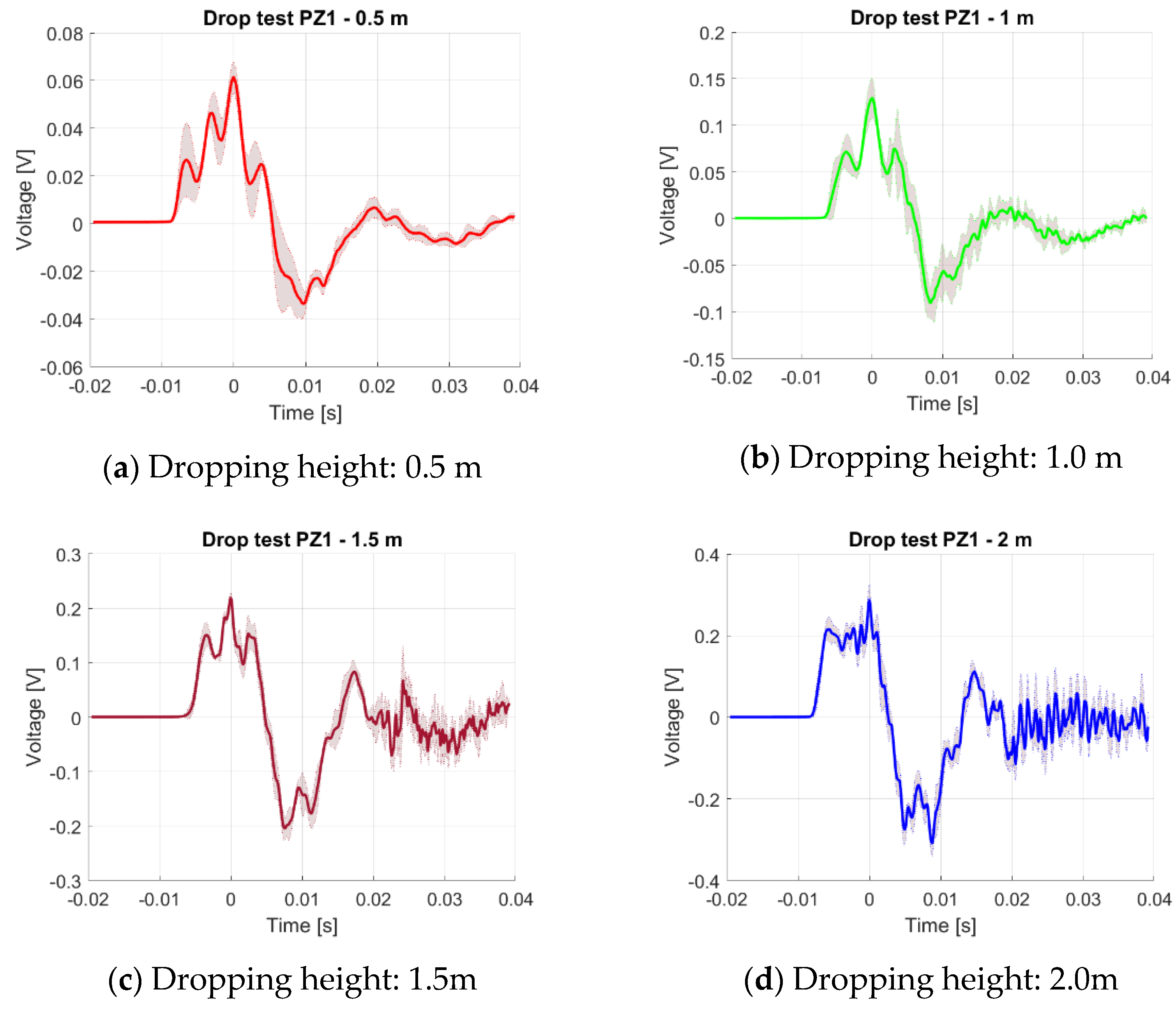
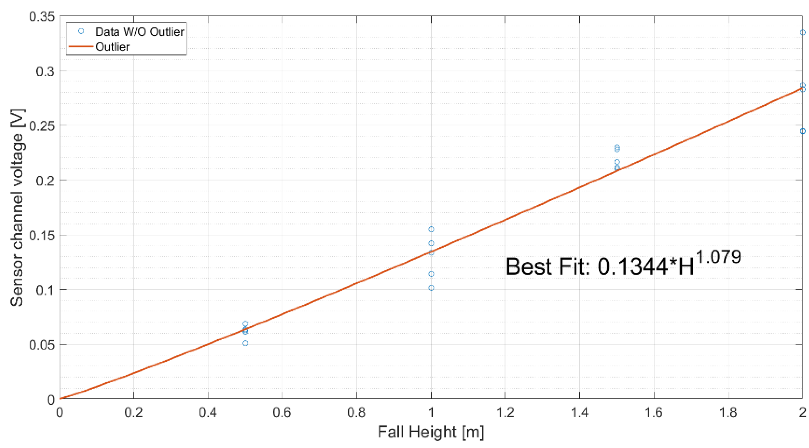
4.4. Drop Tests Results and Analysis

The signals measured by strain gauges, piezoelectric sensors, and fibre optics placed at different locations during impact are influenced by several aspects. Firstly, it is known that the bandwidth of impact force depends on the impactor stiffness. Soft impacts generate smoother responses with longer contacts. Conversely, hard impacts trigger high-frequency responses with small peaks and shorter contact times. Moreover, the structural vibrations produced by the impact occur both on the plate and the dropping object, and are characterized by multiple reflections of stress waves.

Figure 28 and Figure 29 show the strain curves measured at two different locations of impacts from different heights of 0.5 m, 1.0 m, 1.5 m, and 2.0 m, by using strain gauges. The curves plot the mean data and the standard deviation of five consecutive drops from different heights. Due to the insufficiently wide frequency response of the strain gauge bridge, it is evident that such measurements are not affected by high-frequency oscillations caused by the impulsive force. Similarly, the FBG sensor placed near the strain gauge showed similar behaviour, as it can be observed in the results shown in Figure 30. The FBG acquisitions from five consecutive drops at the same height are collected and plotted on the same graph to compare energy levels.

On the contrary, the lamb wave signals caused by the impact are much more affected by the high-frequency components, which, however, have a minor effect, because of the low amplitude and rapid decay. The voltage output from a piezoelectric sensor is shown in Figure 31. The piezo signal, directly generated by the impact, was processed by the charge amplified detailed in Section 4.1, providing a voltage output attenuated by a factor of 100.

The influence of impact velocity on the measured strain responses was also assessed. Due to the different heights, the representative fuel tank was filled with water impacts with the ground, at the velocities of 3.13 m/s; 4.43 m/s, 5.42 m/s, and 6.26 m/s, respectively. The two strain gauges measured a maximum strain of about 250 µε. Additionally, as the impact velocity increases, it can be noted that the impact force takes less time to reach a higher peak value of strain.

Based on these findings, the free drop impact data were used to establish if there is a consistent relation between the maximum sensor signal voltage and the height of the drop. The resulting best fitting curve plot is shown in Figure 32. However, in comparison with numerical predictions, the resulting curve appears dominated by some outliers identified when fitting the curve, which indicates a certain variability in the measurements due to unavoidable experimental errors.

If we assume that the system is linear (constant transfer function for a specific location) and the bandwidth of the input profile generated by the highly flexible dropping object is comparable with that produced by the previously described hammer, the experimental impact profile may also be reconstructed. In the proposed set-up, both impact cases triggered lower frequency responses, and were characterized by relatively high and smooth peaks and a long contact time. Additionally, the duration of impact was proven to be less than the first fundamental natural period of the impacted plate.

5. Conclusions

As a crucial step of a dozen of critical tests before deployment, drop testing plays a central role in the design of crash-resistant flexible fuel tanks. It requires filling the tank with a quantity of water equal to the weight of the maximum fuel load of the tank, and dropping the tank onto a rigid surface. However, although detailed specifications are given to comply with the applicable standards, limited guidelines are available in the literature to support design engineers at the beginning of the design process in both identifying the crashworthiness parameters that play a major role in the mechanical failure, and validating prediction models.

This paper offers useful guidelines for designing and testing a crash-worthy fuel tank. The proposed approach, developed in the framework of the Clean Sky 2 DEFENDER project, has covered a range of activities in an attempt to collect both numerical and experimental data that can help to improve the designing of a flexible fuel tank subjected to full-scale drop tests. Both the simulation and experimental studies have been conducted on a representative test article, consisting of a soft nylon bag filled with water, dropped from different heights onto an instrumented plate equipped with strain gauges, piezoelectric, and fibre Bragg grating sensors. The first phase of the investigation has involved the numerical modelling of the flexible bag filled with liquid and the experimental characterization of the modal properties of the steel plate. These tests were necessary to identify a reliable model needed to reconstruct the impact force via the deconvolution method. The deformation modes of the tank due to drop impacts have been accurately predicted, along with the influence of the liquid sloshing and the strain levels induced on the plate.

Drop test results were satisfactory and gave good agreement to the FE model used. No leakage of liquid or evidence of failures were observed after the impacts. Results indicated that an accurate estimation of the impact force can be obtained by using a transfer function from a single impact, due to a soft tip hammer resulting in smooth peaks and long contact time. From further testing, we also found that the maximum impact force can be correlated with the signals measured by strain gauges and fibre optics. Furthermore, a linear relationship was found between the maximum absolute signal amplitude given by PZT sensors and the maximum impact force. These results expand on previous linear relationships between impact severity (energy or force) and impact signal features (energy, amplitude) proven by similar studies. Finally, among the different achievements of the paper, there is also the validation of both the experimental set-up and the acquisition chain that includes hardware and software tools for monitoring and testing flexible tanks.

Future efforts will be directed toward the impact drop test of the full-scale fuel tank demonstrator and a comprehensive comparison with numerical results predicting the peak impact force, and the influence of further parameters, such as the impact angle and the volume fraction of the water.

References

1. Jackson, K.; Boitnott, R.; Fasanella, E.L.; Jones, L.E.; Lyle, K. A History of Full-Scale Aircraft and Rotorcraft Crash Testing and Simulation at NASA Langley Research Center; BiblioGov: Columbus, OH, USA, 2013. [Google Scholar]
2. Robertson, S.H.; Johnson, N.B.; Hall, D.S.; Rimson, I.J. A Study of Helicopter Crash-Resistant Fuel Systems; Research Report no. DOT/FAA/AR-01/76; Federal Aviation Administration, U.S. Department of Transportation: Washington, DC, USA, 2002.
3. Paciello, C.S.; Pezzella, C.; Belardo, M.; Magistro, S.; Di Caprio, F.; Musella, V.; Lamanna, G.; Di Palma, L. Crashworthiness of a Composite Bladder Fuel Tank for a Tilt Rotor Aircraft. J. Compos. Sci. 2021, 5, 285. [Google Scholar] [CrossRef]
4. Luo, C.; Liu, H.R.; Yang, J.; Liu, K. Simulation and Analysis of Crashworthiness of Fuel Tank for Helicopters. Chin. J. Aeronaut. 2007, 20, 230–235. [Google Scholar] [CrossRef] [Green Version]
5. Yang, X.; Zhang, Z.; Yang, J.; Sun, Y. Fluid–structure interaction analysis of the drop impact test for helicopter fuel tank. SpringerPlus 2016, 5, 1573. [Google Scholar] [CrossRef] [PubMed] [Green Version]
6. Kim, H.-G.; Kim, S. Numerical simulation of crash impact test for fuel cell group of rotorcraft. Int. J. Crashworthiness 2014, 19, 639–652. [Google Scholar] [CrossRef]
7. Lu, G.Y.; Han, Z.J.; Lei, J.P.; Zhang, S.Y. A study on the impact response of liquid-filled cylindrical shells. Thin-Walled Struct. 2009, 47, 1557–1566. [Google Scholar] [CrossRef]
8. Fast Rotorcraft, Clean Sky. Available online: https://www.cleansky.eu/fast-rotorcraft-iadp (accessed on 4 February 2022).
9. Ciminello, M.; De Fenza, A.; Dimino, I.; Pecora, R. Skin-Spar Failure Detection of a Composite Winglet Using FBG Sensors. Arch. Mech. Eng. 2017, 64, 287–300. [Google Scholar] [CrossRef] [Green Version]
10. Abaqus Analysis Guide, version 2020. Available online: http://130.149.89.49:2080/v6.11/books/usb/default.htm (accessed on 1 February 2022).
11. Liu, M.B.; Liu, G.R. Smoothed particle hydrodynamics (SPH): An overview and recent developments. Arch. Comput. Methods Eng. 2010, 17, 25–76. [Google Scholar] [CrossRef] [Green Version]
12. Gingold, R.A.; Monaghan, J.J. Smoothed particle hydrodynamics: Theory and application to nonspherical stars. Mon. Not. R. Astron. Soc. 1977, 181, 375–389. [Google Scholar] [CrossRef]
13. Monoghan, J.J. Smoothed particle hydrodynamics. Annu. Rev. Astron. Astrophys. 1992, 30, 543–574. [Google Scholar] [CrossRef]
14. Monaghan, J.J.; Lattanzio, J.C. A refined particle method for astrophysical problems. Astron. Astrophys. 1985, 149, 135–143. [Google Scholar]
15. Inoue, H.; Watanabe, R.; Shibuya, T.; Koizumi, T. Measurement of impact force by the deconvolution method (part-a). J. Jpn. Soc. Non-Destr. Insp. 1988, 34, 337–342. [Google Scholar]
16. Inoue, H.; Watanabe, R.; Koizumi, T.; Fukuchi, J. Measurement of impact force applied to a plate by the deconvolution method (part-b). J. Jpn. Soc. Non-Destr. Insp. 1988, 37, 874–878. [Google Scholar]
17. Wu, E.; Yeh, J.C.; Yen, C.S. Identification of impact forces at multiple locations on laminated plates. AIAA J. 1994, 32, 2433–2439. [Google Scholar] [CrossRef]
18. Hu, N.; Fukunaga, H.; Yan, B. An efficient approach for identifying impact force using embedded piezoelectric sensors and Chebyshev polynomial. Proc. SPIE—Int. Soc. Opt. Eng. 2005, 6041, 60412Z. [Google Scholar] [CrossRef]
19. Seno, A.H.; Ferri Aliabadi, M.H. A novel method for impact force estimation in composite plates under simulated environmental and operational conditions. Smart Mater. Struct. 2020, 29, 115029. [Google Scholar] [CrossRef]
20. Wu, Z.; Xu, L.; Wang, Y.; Cai, Y. Impact energy identification on a composite plate using basis vectors. Smart Mater. Struct. 2015, 24, 095007. [Google Scholar] [CrossRef]
21. Jang, B.W.; Kim, C.G. Real-time detection of low-velocity impact-induced delamination onset in composite laminates for efficient management of structural health Composites. Smart Mater. Struct. 2017, 123, 124–135. [Google Scholar] [CrossRef]
22. Dung, C.V.; Sasaki, E. Experimental study on impact force identification using output response of polyvinylidene fluoride sensor. Sens. Mater. 2018, 30, 7–21. [Google Scholar]
23. Kalhori, H.; Ye, L.; Mustapha, S.; Li, J.; Li, B. Reconstruction and analysis of impact forces on a steel-beam-reinforced concrete deck. Exp. Mech. 2016, 56, 1547–1558. [Google Scholar] [CrossRef]
24. Xu, L.; Wang, Y.; Cai, Y.; Wu, Z.; Peng, W. Determination of impact events on a plate-like composite structure. Aeronaut. J. 2016, 120, 984–1004. [Google Scholar] [CrossRef]
25. Gunawan, F.E. Levenberg—Marquardt iterative regularization for the pulse-type impact-force reconstruction. J. Sound Vib. 2012, 331, 5424–5434. [Google Scholar] [CrossRef]
26. Presas, A.; Valentin, D.; Egusquiza, E.; Valero, C.; Egusquiza, M.; Bossio, M. Accurate Determination of the Frequency Response Function of Submerged and Confined Structures by Using PZT-Patches. Sensors 2017, 17, 660. [Google Scholar] [CrossRef] [PubMed] [Green Version]
Figure 1. The drop test set-up.
Applmech 03 00020 g001
Figure 2. The sensors’ layout and location.
Applmech 03 00020 g002
Figure 3. The SPH method.
Applmech 03 00020 g003
Figure 4. A schematic representation of a Hugoniot curve.
Applmech 03 00020 g004
Figure 5. The nominal stress vs. nominal strain curve for the flexible tank material.
Applmech 03 00020 g005
Figure 6. The impact surface with supports.
Applmech 03 00020 g006
Figure 7. The FE model of the plate.
Applmech 03 00020 g007
Figure 8. The numerical modal analysis results.
Applmech 03 00020 g008aApplmech 03 00020 g008b
Figure 9. The numerical model adopted for dynamic impact tests.
Applmech 03 00020 g009
Figure 10. The drop test simulations of the representative fuel tank at different times: t = 3 ms, t = 9 ms, t = 15 ms, t = 30 ms. Falling height = 0.5 m. Results: maximum principal strain; global displacements field and global displacement of internal SPH elements.
Applmech 03 00020 g010
Figure 11. The drop test simulations of the representative fuel tank at different times: t = 3 ms, t = 9 ms, t = 15 ms, t = 30 ms. Falling height = 1.0 m. Results: maximum principal strain; global displacements field and global displacement of internal SPH elements.
Applmech 03 00020 g011
Figure 12. The drop test simulations of the representative fuel tank at different times: t = 3 ms, t = 9 ms, t = 15 ms, t = 30 ms. Falling height = 2.0 m. Results: maximum principal strain; global displacements field and global displacement of internal SPH elements.
Applmech 03 00020 g012
Figure 13. The predicted strain time histories for drops from different heights (0.5 m, 1 m and 2 m): (A) strain ε11; (B) strain ε22.
Applmech 03 00020 g013
Figure 14. The best-fitting curve plot of the maximum strain levels predicted on the plate. (a) Fitting of maximum strain ε11 levels, (b) Fitting of maximum strain ε22 levels.
Applmech 03 00020 g014
Figure 15. The displacement’s time history at the upper face tank (global crushing).
Applmech 03 00020 g015
Figure 16. The charge amplifier diagram.
Applmech 03 00020 g016
Figure 17. The charge amplifier electronic board.
Applmech 03 00020 g017
Figure 18. The experimental modal analysis of the instrumented plate.
Applmech 03 00020 g018
Figure 19. The SUM of the acquired FRF (red curve) and MIF (green curve).
Applmech 03 00020 g019
Figure 20. Stabilization diagram using the Polymax plus algorithm.
Applmech 03 00020 g020
Figure 21. The experimental modal shapes up to 180 Hz. (a) Mode 1 @ 47.84 Hz, (b) Mode 2 @ 85.9 Hz, (c) Mode 4 @ 123.0 Hz, (d) Mode 5 @ 124.1 Hz.
Applmech 03 00020 g021
Figure 22. The measured impact force profile.
Applmech 03 00020 g022
Figure 23. The experimental forced and free vibrations in a lamb wave signal caused by impact. (a) zoomed plot, (b) whole signal.
Applmech 03 00020 g023
Figure 24. The linear relation between maximum impact force and maximum response amplitude for impacts tested on the plate.
Applmech 03 00020 g024
Figure 25. The transfer functions measured by the four piezoelectric sensors.
Applmech 03 00020 g025
Figure 26. The transfer function measured by the accelerometer.
Applmech 03 00020 g026
Figure 27. The impact force profiles for different impacts reconstructed by using the transfer function from reference impact H1 at location PZ1.
Applmech 03 00020 g027
Figure 28. The strain time histories measured for drops from different heights (0.5 m, 1.0 m, 1.5 m and 2.0 m) at strain gauge 1 location.
Applmech 03 00020 g028
Figure 29. The strain time histories measured for drops from different heights (0.5 m, 1 m, 1.5 m and 2 m) at strain gauge 2 location from the different heights of 0.5 m, 1.0 m, 1.5 m and 2.0 m.
Applmech 03 00020 g029
Figure 30. The FBG measurements for drops from different heights (0.5 m, 1.0 m, 1.5 m and 2.0 m).
Applmech 03 00020 g030
Figure 31. The voltage output from the piezoelectric sensor PZ1 for drops from different heights (0.5 m (a), 1.0 m (b), 1.5 m (c), and 2.0 m (d)).
Applmech 03 00020 g031
Figure 32. The best fitting curve plot on maximum voltage signal measured by a single piezoelectric sensor.
Applmech 03 00020 g032