A Simple and Effective Method to Evaluate Seismic Maximum Floor Velocities for Steel-Framed Structures with Supplementary Dampers

Abstract

A new method to evaluate the maximum seismic story velocities for steel buildings is examined here. It is well known that story velocities are vital parameters for the design of steel structures with supplementary dampers. It has been recognized that nonlinear time history analysis is required to achieve an accurate evaluation of actual velocities, but this approach seems to be complicated and time-consuming for practical engineers. For this reason, this paper investigates the inelastic velocity ratio, which can be defined as the ratio of the maximum inelastic velocity to the maximum elastic one for steel buildings. The knowledge of this ratio, a unique factor for the whole structure, can be used to evaluate the maximum inelastic story velocities directly from the elastic counterparts. The proposed study is general and can be used in both ordinary steel structures as well as steel structures with supplemental damping devices. Widespread parametric studies are executed to achieve simple yet effective expressions for inelastic velocity ratios.

1. Introduction

According to the philosophy in the traditional seismic design of steel buildings, these structures are designed to resist small earthquake loads by their elastic action only, and the structures are permitted to damage but not collapse while they are subjected to moderate or severe seismic actions (e.g., see EC8 [1]). As a result, plastic hinges in these structures are developed to dissipate the seismic energy when they are under strong ground motions. The design methods based on this philosophy are acceptable to account for the needs of both life safety and economic considerations [2,3,4,5,6]. Nevertheless, the growth of the plastic hinges depends on their high ductility and large deformation. Furthermore, the more ductility the steel-framed structure sustains, the more damage it undergoes. Moreover, some vital steel structures such as museums, fire stations, and hospitals are obliged to endure their functions after a strong ground motion, where the above-mentioned design philosophy based on life safety may not be suitable. These structures must have an adequate amount of strength to avoid large deformation and acceleration so that they can sustain their functions when subjected to strong earthquakes [7,8]. Nevertheless, this design approach allows a guaranteed level of structural damage, which often requires expensive rehabilitation actions. Alternatively, a different possibility to the aforementioned traditional seismic design is the setting up of devices for energy dissipation. The objective of implementing these specific structural components is to offer additional damping and transform it into heat. Thus, the seismic response due to ground motions is decreased through the dissipation of the main portion of seismic energy.

Structural (mainly passive) control systems have been efficiently applied for the design of new structures or the strengthening of older ones. These systems are essential for important buildings such as fire stations, museums, and hospitals to satisfy the preferred seismic performance levels. Characteristic examples of energy dissipation devices are dampers, which have been comprehensively applied in the aerospace and military industry and have in recent times been used in numerous civil structures. There are numerous types of supplementary damping devices:

• Viscous dampers [9,10,11,12,13,14];
• Viscoelastic dampers [15,16];
• Metallic yielding dampers [17,18,19,20];
• Friction dampers [21,22,23,24].

In this study, the most applied cases, those of viscous dampers, are examined. These damping devices are composed of a piston filled with viscous liquid, where its motion leads to energy dissipation [9]. It is worth noting that the damping force of the damper is affected by the velocity and typically provides only viscosity. Despite the decreased response of a structure, inelastic time history analysis is necessary for most structures with supplemental dampers taking into account that a strong ground motion induces an inelastic response for one or more members of the examined structure [7,9]. The most significant parameters in the design of a structure with additional damping devices are the design values of base shear, velocity, and displacement [25,26,27]. It is worth noting that in everyday engineering practice, the maximum (i.e., design) velocity of a building story (hence of the damping devices) is based on the elastic (design) velocity spectra [7,9,25]. Therefore, the real/effective velocity is considered equal to the elastic velocity, assuming the ‘equal velocity rule’, like the familiar ‘equal displacement rule’, which associates the inelastic with the elastic displacement. Nevertheless, since the nonlinear response appears to be unavoidable both for the structures without and with additional damping devices, the elastic velocity spectra cause different velocities in comparison with the effective ones, and consequently, these spectra cannot be adopted. To support this inconsistency, defining the inelastic velocity ratio (IVR) as the ratio of the maximum inelastic velocity to the maximum elastic velocity of a system, Figure 1 depicts the IVR spectra for the behavior factor, q = 4, examining two seismic records.

Thus, in the case that the elastic velocity spectrum undervalues the effective damper velocities (IVR > 1), the ‘equal velocity rule’ seems to be improper since it causes a non-conservative assessment for the damping devices. Conversely, considering that the elastic velocity spectrum overvalues the effective velocity (IVR < 1), which is the case in Figure 1, the hypothesis of the ‘equal velocity rule’ overvalues the damping force, as well as the energy dissipation, leading to an untrue level of seismic performance and, therefore, to over-designed damping devices.

It is worth noting that the hypothesis of IVR = 1.0, as generally held by the modern seismic codes’ provisions, is certainly not conservative. This problematic case becomes obvious through the examination of the total energy of a structure. Thus, the absolute energy equation is given by [7,9]

$$E_I=E_k+E_s+E_h+E_d$$

(1)

where $E_I$ is the earthquake input energy, which corresponds to the energy demand by the seismic event on the structure. Moreover, they have the kinetic energy $E_k$, the elastic strain energy $E_s$, the irreversible hysteretic energy $E_h$, and the energy dissipated by the inherent damping and the probable additional damping devices, $E_d$.

In the case of traditional structures (i.e., without dampers), the term $E_d$ is small. Therefore, adequate structural performance against seismic ground motions is achieved by inherent damping energy, $E_d$, as well as due to the incidence of inelastic behavior, which has to do with the irreversible hysteretic energy, $E_h$. The installation and placement of additional dampers in a structure increase the term $E_d$, in Equation (1), and accounts for the main seismic energy that is absorbed during the seismic event [7,9]. An ideal damping device would be such that the damping force being provided by this does not raise overall internal forces in the structure. Appropriately applied, an idealized damping device should be able to reduce, at the same time, both strain and stress in the structure.

Thus, according to Equation (1) and taking into account that every strong ground motion leads to specific earthquake input energy, the overvalue of effective velocity leads to an overvalue of damping energy and an undervalue of the three other energy terms, i.e., $\left(E_k+E_s+E_h\right)$. Therefore, the assumption of IVR = 1.0 does not seem to be safe and effective for the structures.

The inelastic analysis in the time domain causes an accurate assessment of effective velocities, eliminating the above-mentioned discrepancy. Nevertheless, this method appears to be complicated for most of the practical problems. This study examines an alternative for steel frames to accurately and effectively evaluate the effective velocity. Thus, this paper provides empirical expressions to evaluate the IVR, where its knowledge allows the evaluation of nonlinear velocity directly from the elastic velocity. This method is comparable to the evaluation method and idea of ‘inelastic displacement ratio’, which interrelates the maximum nonlinear and maximum linear elastic displacements [25,28]. Thus, a unique factor, the inelastic velocity ratio, which corresponds to the whole structure, can be used to evaluate all the maximum ‘inelastic’ velocities of stories from the corresponding maximum ‘elastic’ ones. This study can be used for structures without or with additional damping devices. Wide parametric studies are executed to find the empirical equations for the inelastic velocity ratio, in terms of the viscous damping ratio and the fundamental period of vibration.

2. Steel Structures: Description and Analysis

Twelve planar steel moment-resisting frames (MRFs) are examined in this paper. These structures are orthogonal and regular with bay widths and story heights equal to 6 m and 3 m, respectively. Additionally, these frames have several bays n_b with values of 2 and 4 and several stories n_s with values of 3, 6, 9, 12, 15, and 20.

The steel structures have been designed according to Eurocodes EC3 [29] and EC8 [1] provisions. The yield stress of the steel is assumed equal to 275 MPa. The total dead and effective live loads of floors on the beams are set at 25.0 KN/m. The design seismic ground motion was defined by the acceleration design spectrum of EC8, assuming a peak ground acceleration (PGA) equal to 0.30 g and soil class C conditions.

Data of the steel structures, including values for n_s, n_b, beam and column sections, and the fundamental period of vibration, are shown in

Table 1. Steel MRF examined herein.

Frame	ns	nb	Standard Sections (HEB for Columns—IPE for Beams)
1	3	2	240-360(1-3)
2	3	4	240-360(1-3)
3	6	2	280-360(1-4) + 260-360(5-6)
4	6	4	280-360(1-4) + 260-360(5-6)
5	9	2	340-360(1-5) + 320-360(6-7) + 300-330(8-9)
6	9	4	340-360(1-5) + 320-360(6-7) + 300-330(8-9)
7	12	2	400-400(1-5) + 360-400(6-7) + 340-400(8-9) + 340-360(10) + 340-330(11-12)
8	12	4	400-400(1-5) + 360-400(6-7) + 340-400(8-9) + 340-360(10) + 340-330(11-12)
9	15	2	500-450(1-5) + 450-400(6-7) + 400-400(8-12) + 400-360-(13-14) + 400-330(15)
10	15	4	500-450(1-5) + 450-400(6-7) + 400-400(8-12) + 400-360-(13-14) + 400-330(15)
11	20	2	600-450(1-5) + 550-450(6-10) + 500-450(11-13) + 500-400(14-16) + 450-400(17) + 450-360(18-19) + 450-330(20)
12	20	4	600-450(1-5) + 550-450(6-10) + 500-450(11-13) + 500-400(14-16) + 450-400(17) + 450-360(18-19) + 450-330(20)

where expressions of the form 240-330(1-5) + 230-300(6-9) mean that the first five (1–5) stories have columns with HEB240 standard sections and beams with IPE330 standard sections, while the subsequent four (6–9) higher stories have columns with HEB220 standard sections and beams with IPE300 standard sections. For illustrative purposes and without loss of generality, Figure 2 depicts one 6-story and one 15-story planar steel frame, corresponding to Frames No. 3 and No. 9.

A nonlinear multi-degree-of-freedom (MDOF) system with linear damping is assumed for the frames examined here. The equation of motion for these structures can be expressed as [30,31]

$$M\ddot{u}+C\dot{u}+K^{T}u=-M{a}_g$$

(2)

where u is the relative displacement vector and the upper dots stand for time derivatives. Furthermore, M corresponds to the mass matrix, C to the damping matrix, and K^T to the nonlinear stiffness matrix. Additionally, $a_g$ is the acceleration vector of the seismic motion.

The solution of Equation (2) can be found in the time domain using an iterative procedure at every time step using specific software. In this paper, a dynamic inelastic analysis program for framed structures based on the finite element method, the RUAUMOKO program [32], is applied. In the following, a brief explanation of the modeling procedure is presented. Consequently, in this study, a two-dimensional MRF for each steel structure is used to perform an inelastic seismic analysis. The finite element analysis adopts the displacement approach of the structural model. Any frame element has two nodes and each node has three degrees of freedom. Columns and beams are modeled as inelastic frame elements with lumped plasticity using plastic hinges at both ends with the hypothesis of the kinematic linear hardening model with H = 3%, as presented in Figure 3.

Beam axial forces are assumed to be zero since all floors are considered to be rigid to account for the diaphragm action of floor slabs. Characteristic input data for strength that are required by RUAUMOKO [32] are the bending moment M–axial force P interaction diagrams (P-M) for columns (see Figure 4) and bending strength values for beams. It should be mentioned that RUAUMOKO [32] takes into account the variability in the axial force P during seismic events. Beams and columns are connected by rigid joints where the panel zone effects are not modeled. The soil–structure interaction phenomenon is not taken into account, considering fixed base conditions. Second-order effects (P-Δ effects) are taken into account.

The inherent damping ratio, ${\xi }_{inh.}(\%)$, is usually evaluated either by seismic code provisions, e.g., EC8 [1], or by traditional books of Structural Dynamics, e.g., Chopra [30]. In this study, the recently proposed empirical relationship by Cruz and Miranda [33] is adopted to achieve a more accurate estimation, considering that the total height of the structure appears to affect the damped response. Thus, the empirical relationship by Cruz and Miranda [33] is given by Equation (3):

$${\xi }_{inh.}(\%)=\frac{28}{H^{0.52}}$$

(3)

where H is the total height (in meters) of the examined moment-resisting steel frames. Taking into account that all the examined frames appear to have a constant story height, equal to 3.0 m, Figure 5 depicts the inherent damping ratio for these structures in association with their number of stories.

Finally, dampers’ modeling is shown in Figure 6 where characteristic input data for the damping force, F_d, that are required by RUAUMOKO [32] are the damping coefficient C and the exponent value, a, which interrelate damping force with velocity, as shown in Equation (4).

More specifically, viscous dampers are characteristically composed of a piston head with openings enclosed in a tube filled with an extremely viscid fluid, typically a composite of silicone or an analogous kind of oil. Dissipated energy results from piston movement through the viscous fluid. It should be mentioned that viscous dampers were originally applied in the aerospace and military industries, and then they were applied for civil structures in the late-1980s. The behavior of passively damped systems can also be described by the aforementioned model. Thus, according to [7,9], the behavior of viscous fluid dampers can be appropriately expressed by Equation (4):

$$F_d\left(t\right)=c{\left|\dot{u}\left(t\right)\right|}^a·sgn\left(\dot{u}\left(t\right)\right)$$

(4)

where $F_d\left(t\right)$ is the damper’s force, a is an exponent whose value is determined experimentally, and sgn is the signum function.

The physical model corresponding to Equation (4) is a nonlinear viscous dashpot. For earthquake engineering applications, the exponent a typically varies between 0.5 and 1.0 [7,9], where the value a = 1.0 corresponds to a linear viscous dashpot. A non-linear viscous damper for a < 1.0 is effective in decreasing high-velocity shocks. Dampers with a > 1 have not been seen often in practical civil engineering applications. Examining the seismic protection of building structures, many researchers have applied and tested linear viscous dampers [7,9]. Furthermore, in the preliminary analysis and design stages, the velocity exponent of 1.0 is recommended for simplicity. For these reasons and without loss of generality, this paper focuses on the linear viscous dampers, where Equation (4) can also describe the seismic response of passively damped systems. In this case, the maximum damping force, $F_{d,max}$, is given by

$$F_{d,max}=c·{\dot{u}}_{max}$$

(5)

where ${\dot{u}}_{max}$ is the maximum velocity. Since the design of dampers of passively damped structures requires knowledge of the maximum damping force, it is important to determine accurate values for the maximum velocity. This velocity is usually evaluated using the pseudo-velocity spectrum (or from the velocity spectrum), which appears to be an unreliable assumption.

3. Seismic Input

Strong seismic records contain data about the nature of the earthquake shaking and represent all the earthquake motion characteristics, such as duration, energy content, frequency, amplitude, and phase appearances. Real seismic records reproduce all the aspects that affect accelerograms, such as the site path and characteristics of the source. As a result of the increase in accessible earthquake records, applying and scaling real seismic records led to one of the most referenced modern topics in this research field. Regardless of the continual development of the worldwide earthquake records databank, there are numerous combinations of ground motion factors such as site classification, the rupture mechanism source-to-site distance, and the magnitude that are not fine-denoted, which can make finding appropriate records problematic in some situations.

Selected real strong ground motion records are examined to match specific characteristics of the earthquake, commonly based on either a seismic situation, where the minimum parameters are the site classification, distance, and magnitude, or an elastic response spectrum.

The direction given in earthquake design codes on how to select appropriate real records is typically concentrated on the consonance with the response spectrum instead of seismological factors. Consequently, seismic records are adopted based on earthquake factors such as duration, peak ground velocity, and peak ground acceleration to fit a seismic design response spectrum. The seismic records are applied to characterize a severity factor that has to do with a return period or equivalently with a specific hazard level. These selected records should reveal the distance, site condition, magnitude, and other factors that affect the seismic characteristics. The selection of seismic records corresponding to suitable magnitudes is vital for the reason that magnitude intensely affects the duration of ground motion as well as the content of frequencies. It is required to adopt seismic events with magnitudes very close to the target magnitude [8,25,26]. The choice of seismic records having proper distances from the fault site is vital particularly for near-fault locations, for the reason that the physiognomies of near-fault records vary from those of far-field records. Additionally, site conditions appear to have a key role in the physiognomies and content of frequencies of the seismic records. Thus, in soft soils, high-frequency motions are decreased although the seismic motions are generally enlarged. Usually, the seismic motion magnification consequence can be found in the spectral acceleration at intermediate to short frequencies.

In the following, the seismic record scaling is examined. In this case, the seismic record can be regularly scaled down or up to fit the target response spectrum, leaving the content of frequencies unaffected, within a frequency range of interest. In this research study, where numerous time histories are examined, each record has a specific scale factor to ensure that the peak ground acceleration of the design spectrum and each record are identical.

A group of 25 accelerograms, which is selected with the above-mentioned criteria, is shown in

Table 2. Recorded far-fault earthquake ground motions, which correspond to stiff soil.

No.	Date	Record Name	Comp.	Station Name	PGA (g)
1	20 September 1999	Chi-Chi, Taiwan	NS	NST	0.388
2	20 September 1999	Chi-Chi, Taiwan	EW	NST	0.309
3	2 May 1983	Coalinga	EW	36227 Parkfield	0.147
4	2 May 1983	Coalinga	NS	36227 Parkfield	0.131
5	12 November 1999	Duzce, Turkey	NS	Bolu	0.728
6	12 November 1999	Duzce, Turkey	EW	Bolu	0.822
7	15 October 1979	Imperial Valley	N015	6622 Compuertas	0.186
8	15 October 1979	Imperial Valley	N285	6622 Compuertas	0.147
9	15 October 1979	Imperial Valley	N012	6621 Chihuahua	0.270
10	15 October 1979	Imperial Valley	N282	6621 Chihuahua	0.284
11	17 August 1999	Kocaeli, Turkey	NS	Atakoy	0.105
12	17 August 1999	Kocaeli, Turkey	EW	Atakoy	0.164
13	18 October 1989	Loma Prieta	NS	1028 Hollister City Hall	0.247
14	18 October 1989	Loma Prieta	EW	1028 Hollister City Hall	0.215
15	24 April 1984	Morgan Hill	NS	57382 Gilroy Array #4	0.224
16	24 April 1984	Morgan Hill	EW	57382 Gilroy Array #4	0.348
17	17 January 1994	Northridge	NS	90057 Canyon Country	0.482
18	17 January 1994	Northridge	EW	90057 Canyon Country	0.410
19	9 February 1971	San Fernando	EW	135 LA—Hollywood	0.210
20	9 February 1971	San Fernando	NS	135 LA—Hollywood	0.174
21	26 April 1981	Westmorland	NS	5169 Westmorland Fire Sta	0.368
22	26 April 1981	Westmorland	EW	5169 Westmorland Fire Sta	0.496
23	24 November 1987	Superst. Hills (B)	NS	01335 El Centro Imp. Co. Cent	0.258
24	24 November 1987	Superst. Hills (B)	EW	01335 El Centro Imp. Co. Cent	0.358
25	27 January 1980	Livermore	EW	57187 San Ramon	0.301

. For more information, one can consult the work of Hatzigeorgiou [34], from where the set of records under consideration has been adopted.

All these records correspond to stiff soil, i.e., to soil type C, according to EC8 [1], to be compatible with the steel frames’ design. The complete list of these earthquakes was downloaded from the strong motion database of the Pacific Earthquake Engineering Research (PEER) Center where the mean pseudo-acceleration spectra for viscous damping ratios ξ = 5% are presented in Figure 7.

4. Proposed Methodology

In the following, the proposed methodology to assess the inelastic velocities of steel building structures is analyzed:

• STEP 1:

Compute (or estimate using appropriate empirical expressions from the pertinent literature) the fundamental period, T, of the steel building structure under consideration.

• STEP2:

From preliminary free-damped vibration analysis, evaluate the equivalent viscous damping ratio, ξ_eq., for the steel building structure with supplementary dampers.

• STEP 3:

Evaluate the inelastic velocity ratio, IVR, using the following empirical expression:

$$IVR\left(q,T\right)=1+{\left(q-1\right)}^a\left(\frac{b}{T^{0.9}}+\frac{c}{T}\right)$$

(6)

where q is the behavior factor of the structure assuming this factor for the design earthquake, and a, b, and c are parameters whose values appear in

Table 3. IVR parameters.

Parameter	a	b	c
ξeq = 5%	0.35069	−1.43800	1.23579
ξeq = 10%	0.45772	−1.23279	1.08484
ξeq = 20%	0.54494	−0.87169	0.77337
ξeq = 30%	0.55136	−0.69468	0.61634
ξeq = 40%	0.60285	−0.55529	0.49353
ξeq = 50%	0.59042	−0.49497	0.44038

.

A complete regression analysis is implemented using the databank obtained through the aforementioned nonlinear time history analyses. The influence of the fundamental period of vibration and behavior factors on IVR is taken into account. The results from the databank are used in association with Table Curve 3D [35] where the empirical relation of Equation (5) is chosen, considering its great simplicity and efficiency.

• STEP 4:

Evaluate the maximum values of inelastic inter-story velocities from their elastic counterparts (i.e., from the elastic analysis results) by multiplying the last ones by the IVR.

5. Verification and Applications

In this section, two steel planar frames, having 3 bays and 3 and 9 stories, are examined, which have been designed according to EC8 [1] for q = 4. The adopted steel sections are shown in Table 1. Two equivalent damping ratios, i.e., ξ_eq = 5% and 30%, are examined. Figure 8 and Figure 9 depict the profiles of inter-story mean velocities for the whole set of 25 earthquakes of Table 2 and for the following cases: (a) elastic analysis, (b) inelastic analysis using time-history responses, and (c) inelastic values from elastic analysis using IVR.

The proposed method can reliably estimate the inelastic inter-story velocities using the linear counterpart and inelastic velocity ratios (IVRs), both for 3-story and 9-story frames and for the equivalent damping values of 5% and 30%. Therefore, the proposed method can be used by adopting the elastic analysis values, avoiding complicated, nonlinear, and time-consuming methods. Furthermore, it is evident that elastic velocities appear to be different in comparison with their inelastic counterparts and, therefore, the assumption of IVR = 1.0 seems to be baseless.

Finally, Figure 10 presents the ratio of V_PR/V_NTHA, which has to do with the predicted maximum story velocities, V_PR, using the inelastic velocity ratio, and the maximum story velocities result from nonlinear time history analysis, V_NTHA. This figure depicts the whole sample of structures (maximum velocity for all stories) under the action of a whole set of 25 earthquakes under consideration. The V_PR/V_NTHA ratio is more or less equal to 1.0; i.e., the predicted maximum velocities using the inelastic velocity ratio are almost identical to those resulting from seismic inelastic time-history analyses. Therefore, the proposed method appears to be reliable and accurate.

6. Conclusions

This paper examined a new approach for the reliable estimation of actual velocities of inelastic planar steel-framed structures under strong ground motions. The proposed methodology has to do with the inelastic velocity ratio, which can be defined as the ratio of the maximum inelastic to the maximum elastic velocity, where its knowledge allows the computation of maximum inelastic story velocities directly from the corresponding elastic ones. The application of the inelastic velocity ratio for seismic analysis of steel structures is applied for the first time in this study. After applications, the following conclusions can be drawn:

• It seems impermissible and inaccurate to assume that the inelastic velocity ratio is equal to unity, i.e., that the inelastic velocities are equal to the corresponding elastic ones.
• The proposed research study is simple and straightforward, without increased computational cost.
• Numerous inelastic time-history analyses were carried out and a comprehensive nonlinear regression analysis was carried out to provide simple empirical expressions for the inelastic velocity ratio. The influence of the fundamental period of vibration and the equivalent viscous damping ratio is taken into account.
• This method appears to be useful both for traditional steel frames and for steel frames with supplementary dampers.
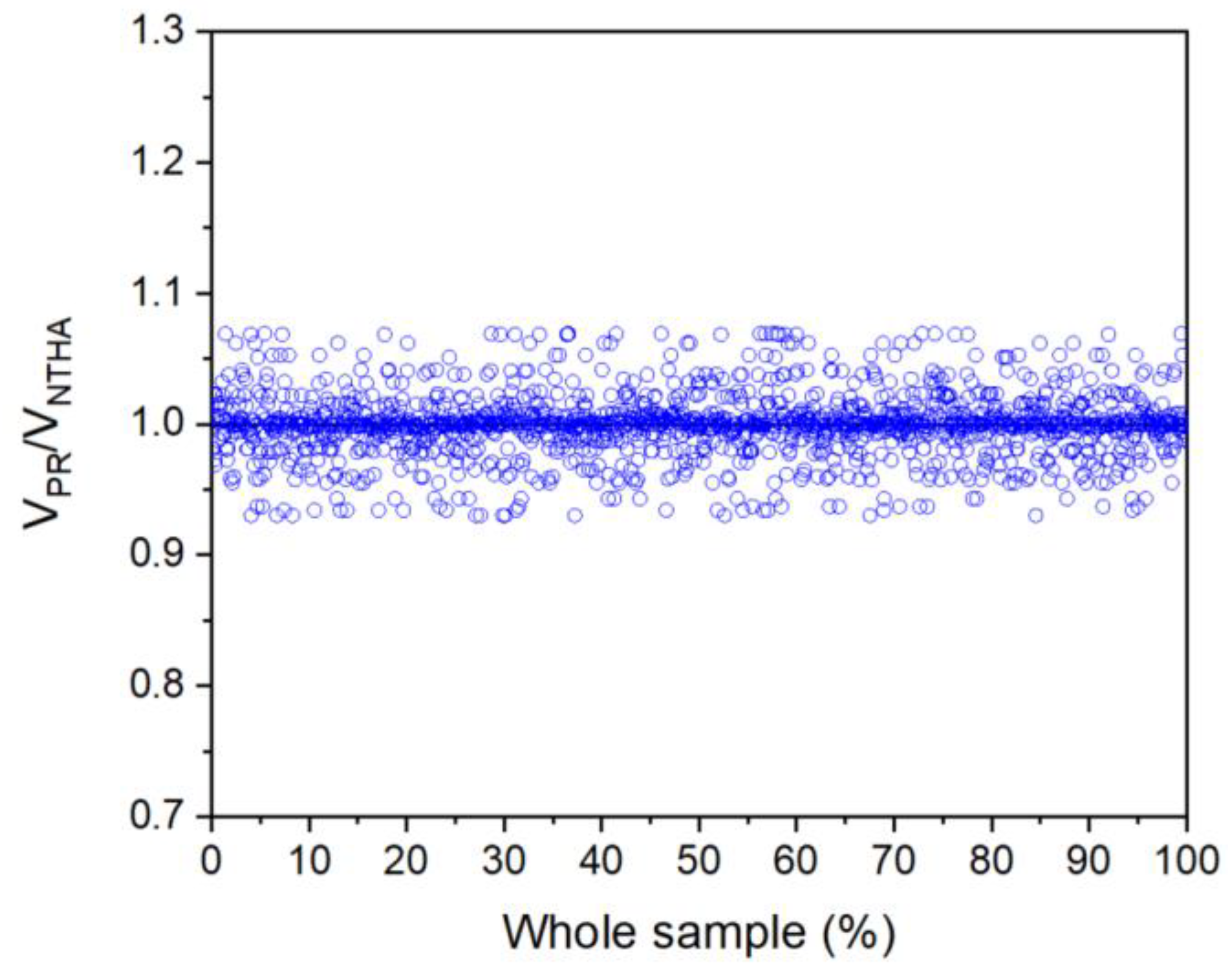
• Comparing the proposed method with dynamic inelastic time history analyses, it is found that the proposed study appears to be reliable and accurate.

References

1. EN1998-1; Eurocode 8: Design of Structures for Earthquake Resistance―Part 1: General rules, Seismic Actions, and Rules for Buildings. European Committee for Standardization: Brussels, Belgium, 2005.
2. Uang, C.M.; Bruneau, M. State-of-the-art review on seismic design of steel structures. J. Struct. Eng. 2018, 144, 03118002. [Google Scholar] [CrossRef]
3. Fang, C.; Wang, W.; Qiu, C.; Hu, S.; MacRae, G.A.; Eatherton, M.R. Seismic resilient steel structures: A review of research, practice, challenges and opportunities. J. Constr. Steel Res. 2022, 191, 107172. [Google Scholar] [CrossRef]
4. Zhang, Z.; Shen, H.; Wang, Q. Constant ductility inelastic displacement ratio spectra of shape memory alloy-friction self-centering structures based on a hybrid model. Bull. Earthq. Eng. 2023, 21, 927–956. [Google Scholar] [CrossRef]
5. Sarcheshmehpour, M.; Estekanchi, H.E.; Ghannad, M.A. Optimum placement of supplementary viscous dampers for seismic rehabilitation of steel frames considering soil–structure interaction. Struct. Des. Tall Spec. Build. 2020, 29, e1682. [Google Scholar] [CrossRef]
6. Zhang, R.; Chu, S.; Sun, K.; Zhang, Z.; Wang, H. Effect of the directional components of earthquakes on the seismic behavior of an unanchored steel tank. Appl. Sci. 2020, 10, 5489. [Google Scholar] [CrossRef]
7. Hatzigeorgiou, G.D.; Papagiannopoulos, G.A. Inelastic velocity ratio. Earthq. Eng. Struct. Dyn. 2012, 41, 2025–2041. [Google Scholar] [CrossRef]
8. Hatzigeorgiou, G.D. Ductility demands control under repeated earthquakes using appropriate force reduction factors. J. Earthq. Tsunami 2010, 4, 231–250. [Google Scholar] [CrossRef]
9. Hatzigeorgiou, G.D.; Pnevmatikos, N.G. Maximum damping forces for structures with viscous dampers under near-source earthquakes. Eng. Struct. 2014, 68, 1–13. [Google Scholar] [CrossRef]
10. Bakhshinezhad, S.; Mohebbi, M. Multi-objective optimal design of semi-active fluid viscous dampers for nonlinear structures using NSGA-II. Structures 2020, 24, 678–689. [Google Scholar] [CrossRef]
11. Moradpour, S.; Dehestani, M. Optimal DDBD procedure for designing steel structures with nonlinear fluid viscous dampers. Structures 2019, 22, 154–174. [Google Scholar] [CrossRef]
12. Silwal, B.; Ozbulut, O.E.; Michael, R.J. Seismic collapse evaluation of steel moment resisting frames with superelastic viscous damper. J. Constr. Steel Res. 2016, 126, 26–36. [Google Scholar] [CrossRef]
13. Kim, J.; Lee, J.; Kang, H. Seismic retrofit of special truss moment frames using viscous dampers. J. Constr. Steel Res. 2016, 123, 53–67. [Google Scholar] [CrossRef]
14. Constantinou, M.C.; Symans, M.D. Experimental study of seismic response of buildings with supplemental fluid dampers. Struct. Des. Tall Build. 1993, 2, 93–132. [Google Scholar] [CrossRef]
15. Shu, Z.; Ning, B.; Li, S.; Li, Z.; Gan, Z.; Xie, Y. Experimental and numerical investigations of replaceable moment-resisting viscoelastic damper for steel frames. J. Constr. Steel Res. 2020, 170, 106100. [Google Scholar] [CrossRef]
16. Lai, M.L.; Chang, K.C.; Soong, T.T.; Hao, D.S.; Yeh, Y.C. Full-scale viscoelastically damped steel frame. J. Struct. Eng. 1995, 121, 1443–1447. [Google Scholar] [CrossRef]
17. Tremblay, R.; Bolduc, P.; Neville, R.; DeVall, R. Seismic testing and performance of buckling-restrained bracing systems. Can. J. Civ. Eng. 2006, 33, 183–198. [Google Scholar] [CrossRef]
18. Garivani, S.; Aghakouchak, A.A.; Shahbeyk, S. Numerical and experimental study of comb-teeth metallic yielding dampers. Int. J. Steel Struct. 2016, 16, 177–196. [Google Scholar] [CrossRef]
19. Tsai, K.C.; Chen, H.W.; Hong, C.P.; Su, Y.F. Design of steel triangular plate energy absorbers for seismic-resistant construction. Earthq. Spectra 1993, 9, 505–528. [Google Scholar] [CrossRef]
20. Kelly, J.M.; Skinner, R.I.; Heine, A.J. Mechanisms of energy absorption in special devices for use in earthquake resistant structures. Bull. New Zealand Soc. Earthq. Eng. 1972, 5, 63–88. [Google Scholar] [CrossRef]
21. Francavilla, A.B.; Latour, M.; Piluso, V.; Rizzano, G. Design criteria for beam-to-column connections equipped with friction devices. J. Constr. Steel Res. 2020, 172, 106240. [Google Scholar] [CrossRef]
22. Bagheri, S.; Barghian, M.; Saieri, F.; Farzinfar, A. U-shaped metallic-yielding damper in building structures: Seismic behavior and comparison with a friction damper. Structures 2015, 3, 163–171. [Google Scholar] [CrossRef]
23. Grigorian, C.E.; Yang, T.S.; Popov, E.P. Slotted bolted connection energy dissipators. Earthq. Spectra 1993, 9, 491–504. [Google Scholar] [CrossRef]
24. Pall, A.S.; Marsh, C. Response of friction damped braced frames. J. Struct. Div. 1982, 108, 1313–1323. [Google Scholar] [CrossRef]
25. Dong, H.; Han, Q.; Qiu, C.; Du, X.; Liu, J. Residual displacement responses of structures subjected to near-fault pulse-like ground motions. Struct. Infrastruct. Eng. 2022, 18, 313–329. [Google Scholar] [CrossRef]
26. Muho, E.V.; Qian, J.; Beskos, D.E. Modal behavior factors for the performance-based seismic design of R/C wall-frame dual systems and infilled-MRFs. Soil Dyn. Earthq. Eng. 2020, 129. [Google Scholar] [CrossRef]
27. Desai, R.; Tande, S. Estimate of peak relative velocity from conventional spectral velocity for response spectrum based force evaluation in damping devices. Structures 2018, 15, 378–387. [Google Scholar] [CrossRef]
28. Dong, H.; Han, Q.; Du, X.; Liu, J. Constant ductility inelastic displacement ratios for the design of self-centering structures with flag-shaped model subjected to pulse-type ground motions. Soil Dyn. Earthq. Eng. 2020, 133, 106143. [Google Scholar] [CrossRef]
29. EN 1993-1-1; Eurocode 3—Design of Steel Structures—Part 1-1: General Rules and Rules for Buildings. European Committee for Standardization: Brussels, Belgium, 2002.
30. Chopra, A.K. Dynamics of Structures; Pearson Prentice Hall: Berkeley, CA, USA, 2007. [Google Scholar]
31. Humar, J. Dynamics of Structures; CRC Press: London, UK, 2012. [Google Scholar]
32. Carr, A.J. RUAUMOKO-2D Inelastic Time-History Analysis of Two-Dimensional Framed Structures; Department of Civil Engineering, University of Canterbury: Christchurch, New Zealand, 2008. [Google Scholar]
33. Cruz, C.; Miranda, E. Damping ratios of the first mode for the seismic analysis of buildings. J. Struct. Eng. 2021, 147, 04020300. [Google Scholar] [CrossRef]
34. Hatzigeorgiou, G.D. Damping modification factors for SDOF systems subjected to near-fault, far-fault, and artificial earthquakes. Earthq. Eng. Struct. Dyn. 2010, 39, 1239–1258. [Google Scholar] [CrossRef]
35. Systat Software, Inc. TableCurve 3D. 2023. Available online: https://systatsoftware.com/tablecurve3d/ (accessed on 2 January 2023).
Figure 1. Inelastic velocity ratio for two strong ground motions and q = 4.
Applmech 04 00057 g001
Figure 2. Examples of planar steel frames examined here.
Applmech 04 00057 g002
Figure 3. Bilinear elastoplastic hysteretic model.
Applmech 04 00057 g003
Figure 4. P-M interaction diagram (Carr, [32]).
Applmech 04 00057 g004
Figure 5. Inherent damping ratio as a function of the number of stories for the steel moment-resisting frames under consideration.
Applmech 04 00057 g005
Figure 6. Viscous damper’s model (adapted from [32]).
Applmech 04 00057 g006
Figure 7. Accelerogram spectra, mean spectrum, and design spectrum EC8 [1].
Applmech 04 00057 g007
Figure 8. Profiles of inter-story velocities for a 3-story building for ξeq. = 5% (left) and 30% (right).
Applmech 04 00057 g008
Figure 9. Profiles of inter-story velocities for 9-story building for ξeq. = 5% (left) and 30% (right).
Applmech 04 00057 g009
Figure 10. Predicted vs. ’exact’ maximum story velocities: VPR/VNTHA ratio.
Applmech 04 00057 g010