Automated Long-Term Stability of a High-Energy Laser

Abstract

We present a method for regulating the laser energy output with a software-controlled waveplate–polariser configuration. By implementing this technology, we have effectively eliminated energy output fluctuations over time, allowing for the laser to reach its nominal energy up to 2 h earlier. Our testing demonstrates a stability of 2.8% (RMS), verifying the system’s reliability. We provide an overview of the software and its basic operation, along with practical evidence of the system’s efficacy in maintaining a stable laser energy output.

1. Introduction

In this article, we describe a method to stabilise the output energy of an initially unstable laser within a complex laser system. Similar techniques have been implemented in different situations [1].

We discovered for the laser used in our system that the output energy varies over the course of the day, specifically with a significantly higher energy output at the beginning of the day, before levelling off to a more stable operational level. This warm-up period, to a point where the output is more stable, is around two hours, and is believed to be due to thermal effects inside the laser.

This warm-up time is problematic since the laser is the pump laser of an Optical Parametric Chirped Pulse Amplification (OPCPA) system [2,3,4,5]; these are inherently sensitive to the energy of the pump pulse, with the output energy varying exponentially with the input pump energy away from saturation, and linearly thereafter. In order to maintain a stable energy output of the OPCPA system, we must be pumping with a laser of constant energy. OPCPA depends on other factors aside from the pump energy, such as temporal overlapping of the seed and pump, the phase-matching angle between the seed and pump, and the intensity of each pulse. In order to maximise the stability of a system, each of these conditions needs to be satisfied and controlled. However, away from saturation, the exponential dependence of the pump intensity makes it the most important parameter to control in order to maintain a stable energy output. We investigate only the effect of this technology on the laser itself, and do not present any results relating to an increased stability in the entire laser system of which this pump is one part. With the advent of new scientific facilities that use OPCPA incorporated in their systems coming online [6,7,8,9], stabilization of the pump energy is crucial. Moreover, we can envision that this same system could be applied to a wide range of lasers as long as they are not single-shot lasers. In fact, applications from 3D printing [10] to laser plasma accelerators [11] or shearography [12] imply a careful control of the laser energy; this is especially problematic for low-repetition-rate, high-energy lasers [13,14] that perform intricate, highly nonlinear physics at the same time as comporting a high thermal load that is due to changes in the environment, and also due to the heating of the laser components during pumping. A full description of the sub-system this pump laser is included in can be found in [2].

As such, we present the work undertaken to regulate the energy of this laser by varying the polarisation of the pulses before it is redefined later on in the laser cavity. We believe this technique could be easily implemented in any complex laser system where a constant pump energy is an important factor.

2. Method and Code Logic

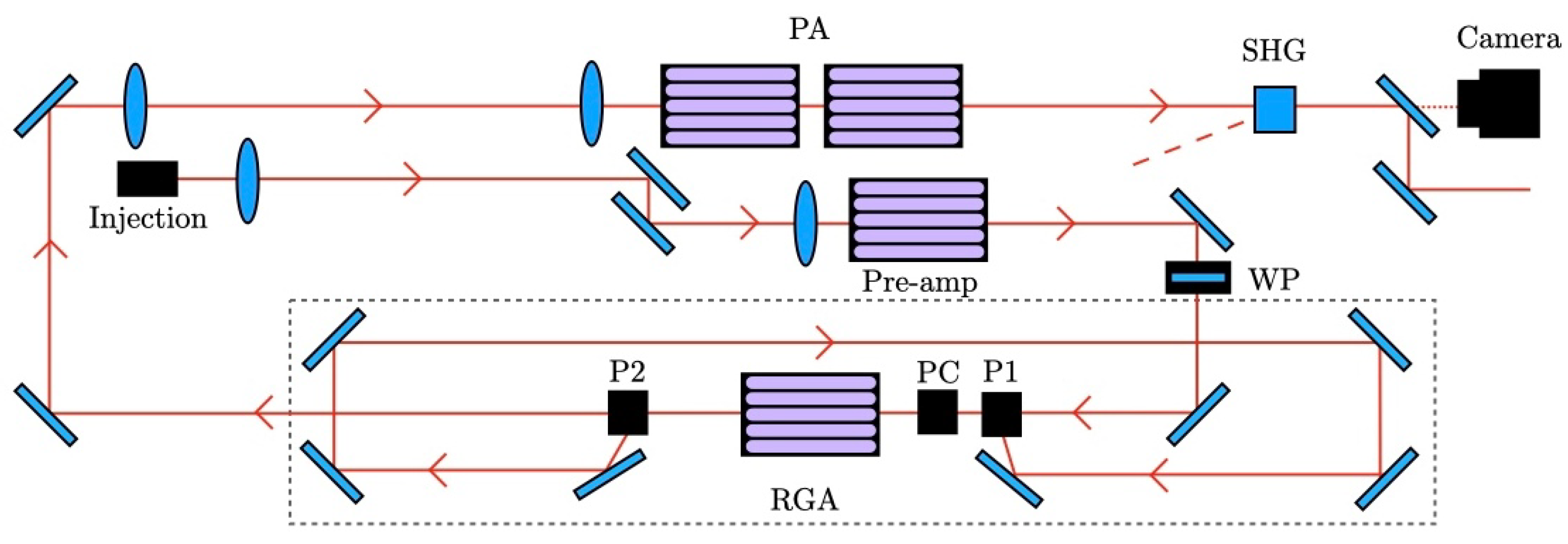
Figure 1 shows a schematic of the laser cavity.

A laser temporally shaped by a fibre EOM is delivered by fibre to the amplification system. It is then magnified to match the pre-amplifier size of 5 mm (the amplifier diameter is 6 mm) with a gain of 20. Our energy control waveplate (WP) is after the pre-amplifier and before injection into a regenerative amplifier with an SSG of 20 per pass with relay imaging and a pinhole in the far-field. Therefore, the power incident on the WP is low. The output energy is 30 mJ at the output of the amplifier, which is then magnified with a positive–negative telescope to a 12 mm diameter before passing to the power amplifiers, which amplify it to 1 J; this is converted to the second harmonic using a KDP crystal for an output energy of 0.5 J. The pulse duration is 4.5 ns and the repetition rate is 2 Hz.

The output of the laser is monitored by a camera (in our case a uEye USB camera) and controlled by the movement of a $\lambda /2$ waveplate, which is mounted on a motorised rotational mount purchased from ThorLabs (Model KDC101). The energy is calculated by averaging the reading from each pixel in the acquired image. A camera is used due to its sensitivity at low energies, low cost, and ability to encompass the entirety of the beam. Alternative sensors could include a wide sensor photo-diode, or a more costly solution could be a calibrated Gentec energy sensor.

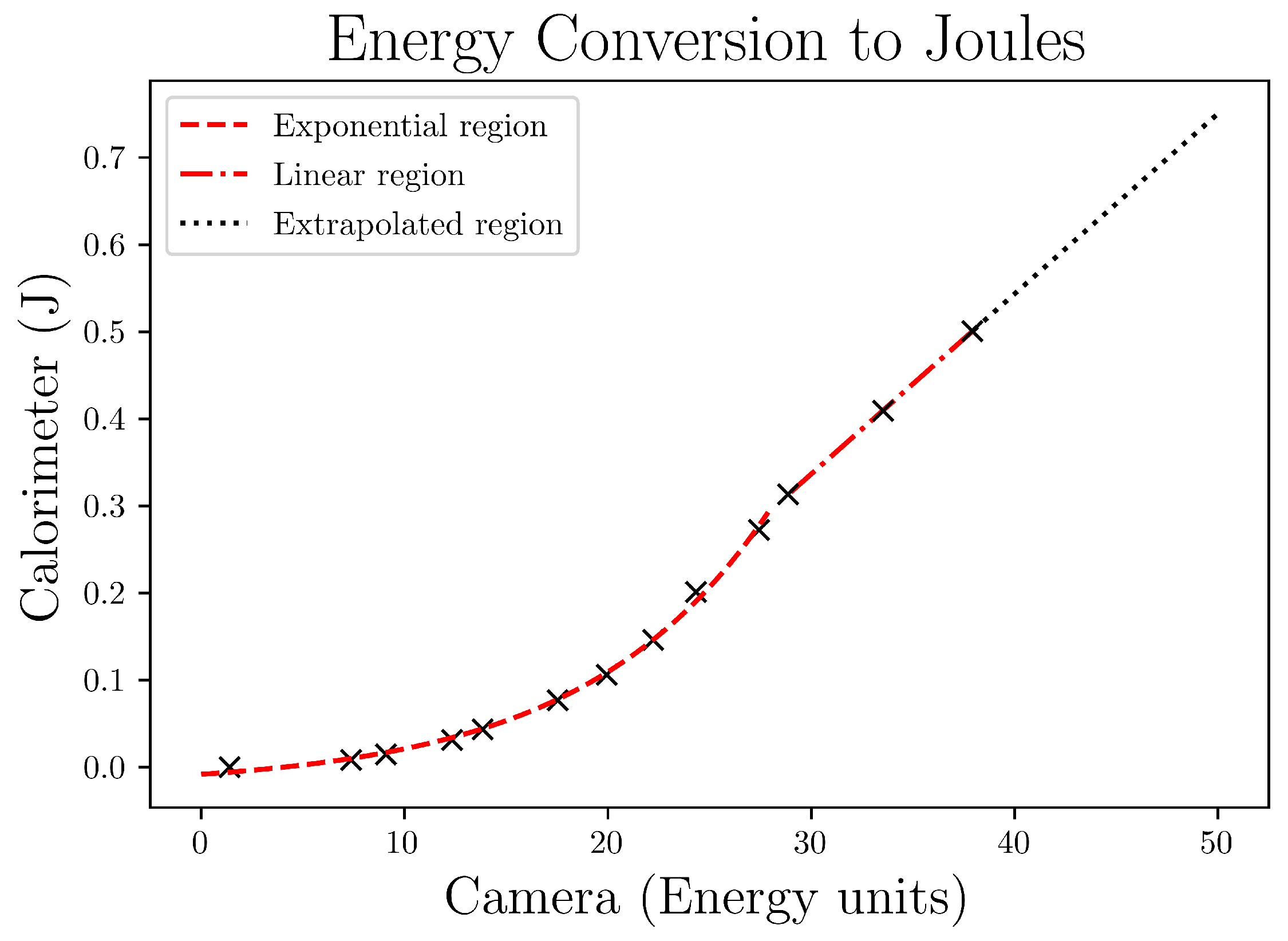
To convert energy measurements in camera units to Joules, measurements of the pump energy in the system were taken with a calorimeter. By obtaining an average energy with the camera and with the calorimeter for multiple set energies, one is able to determine the camera’s calorimetry response (see Figure 2). We found this function to be non-linear for low energies and well approximated to the piecewise function:

$$\left\{\begin{array}{cc}0.0145\times exp\left(0.1104x\right)-0.0228,\hfill & x<27.89,\hfill \\ 0.0207x-0.2843,\hfill & x\ge 27.89\hfill \end{array}\right.$$

(1)

with x being the camera energy and the output in Joules. The rms errors for the fit in the exponential and linear regions are 4.4 mJ and 0.3 mJ, respectively.

Giving the software a calibration function (see Section 2.2) and a set energy, it is able to move the WP to a calculated angle, which, after altering the polarisation in turn, changes the transmission through the polariser. For a standard $\lambda /2$ waveplate, we would expect the transmission through the polariser to follow a sinusoidal-squared curve as per the well-known Malus’ Law.

However, a theoretical curve of this form could not be used in our case due to the presence of amplifiers in between the control and detection devices, as well as a non-linear camera calorimetry response (see Figure 1 and Figure 2). This adds complication which would be impractical to formulate in this case, since, as in most real-world situations with a feedback loop, a practical calibration serves as a more accurate method for optimising the response. As such, we used a polynomial of order 3 due to its good fit to the calibration data.

2.1. Calculating the New Angle

Many forms of feedback loop exist, each with their own benefits and drawbacks depending on the situation. For example, a simple proportional p-loop could be used to minimise the error, $\epsilon =\mathrm{Measured}\mathrm{Energy}-\mathrm{Setpoint}\mathrm{Energy}$. Instead, we decided to use a method whose next guess is calculated so as to converge to the correct value very rapidly. In some circumstances, e.g., where a very short loop time is desired, this method may be too computationally intensive. However, there were no concerns of this nature here as the repetition rate of the oscillator itself is (only) 2 Hz, slow enough for a computer to complete this calculation and be ready to go again. Furthermore, it is much more important to converge rapidly when the feedback loop time is larger, simply because fewer iterations occur for a given time period. Therefore, for our system to have a fast response to change and minimise the presence of instability in the output, the following method was selected.

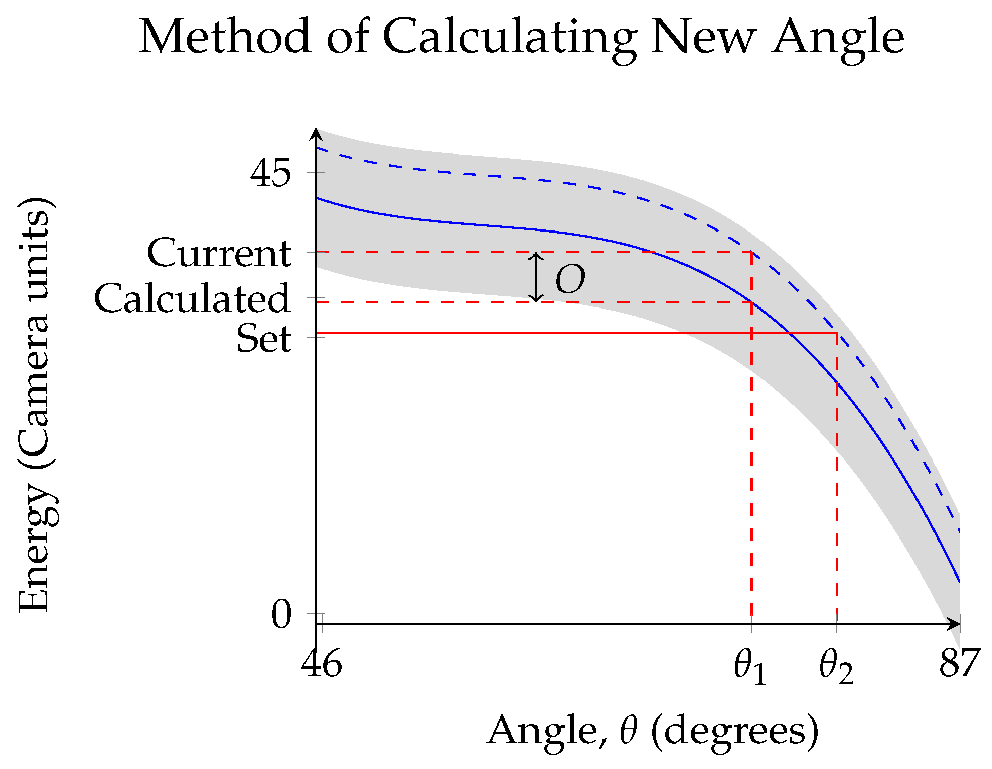
First, an image is acquired from the camera, and a value for the current energy $E_{\mathrm{cur}}$ (labelled ‘Current’ in Figure 3) is computed.

Next, a calculation of the energy is made from the calibration function, $f\left(\theta \right)$, using the current angle (labelled ‘Calculated’ in Figure 3), which is given by

$$\begin{array}{c}\hfill E_{\mathrm{calc}}=A·{\theta }_{\mathrm{cur}}^3+B·{\theta }_{\mathrm{cur}}^2+C·{\theta }_{\mathrm{cur}}+D,\end{array}$$

(2)

where $E_{\mathrm{calc}}$ is the calculated energy, ${\theta }_{\mathrm{cur}}$ is the current angle, and $A,B,C,D$ are the calibration function coefficients. This then gives a value for the offset O, which as Figure 3 shows is the difference between the theoretical value we would expect from the calibration function and the value we actually measure:

$$\begin{array}{c}\hfill O=E_{\mathrm{cur}}-E_{\mathrm{calc}}.\end{array}$$

(3)

This can be visualised as a translation of the calibration function to a new position, where the translation is exactly equal to O.

We then define an updated calibration function $\widehat{f}\left(\theta \right):=f\left(\theta \right)+O$, equal to the dashed blue curve in Figure 3. From this, we solve for ${\theta }_2$, which is to be our calculated angle, by finding the value of theta such that $\widehat{f}\left(\theta \right)=\mathrm{Set}\mathrm{Energy}$, i.e.,

$$\begin{array}{c}\hfill A·{\theta }^3+B·{\theta }^2+C·\theta +(D-O-\mathrm{Set}\mathrm{Energy})=0.\end{array}$$

(4)

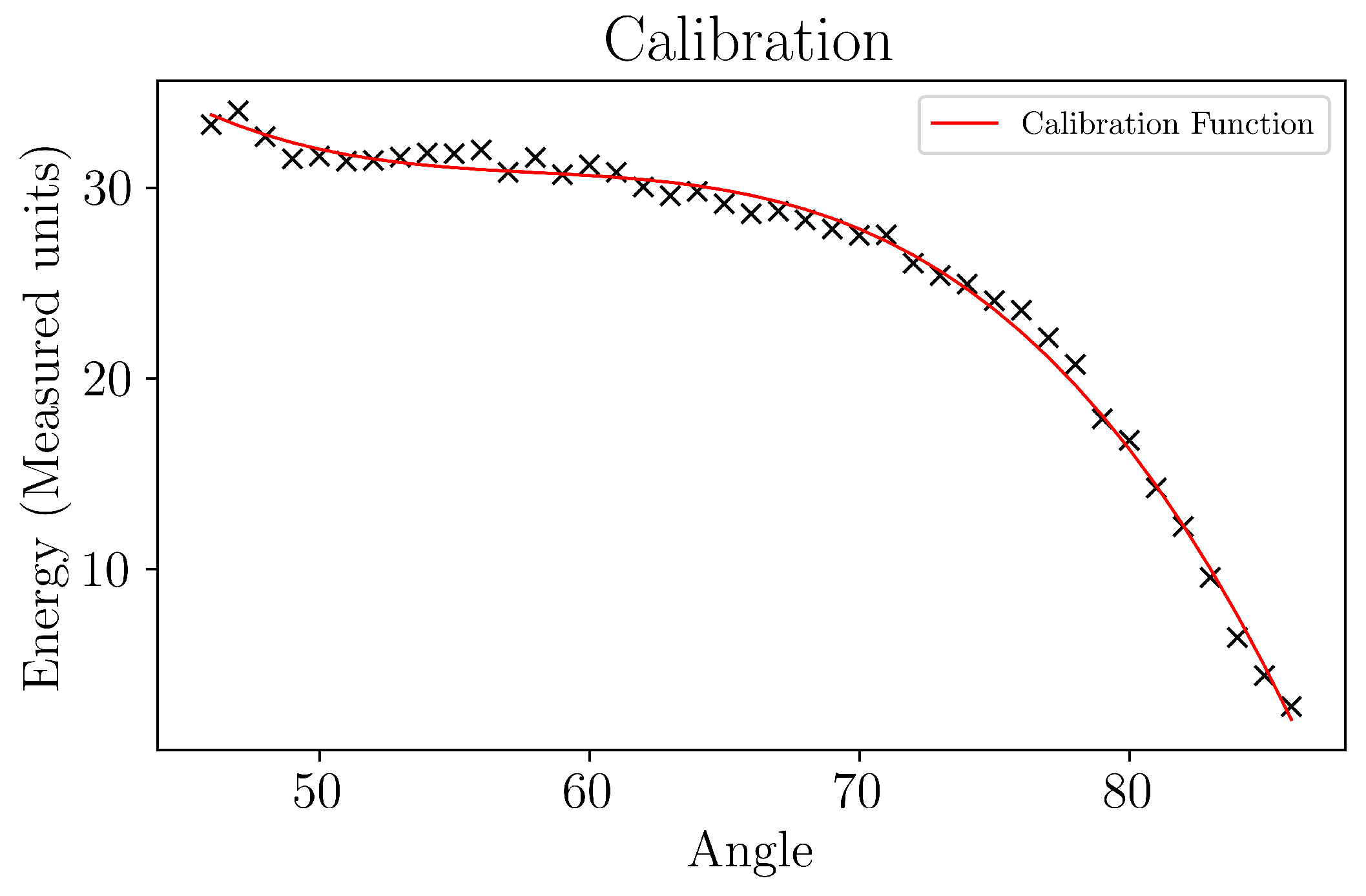
A correct calibration function will only lead to one real solution in the range $[{\theta }_i,{\theta }_f]$, which is the angle (${\theta }_2$) the WP is commanded to move to. Please note how well the cubic function fits in Figure 4.

2.2. Obtaining a Calibration Function

The method in the previous section only yields useful values when an appropriate calibration function is provided. This software, written in C#, has the functionality of self-calibration. To obtain a valid calibration curve, an energy scan taken over a short time scale (relative to any drifts in the laser output) is taken. In our case, the scan takes approximately 2 min. The scan commences at the smallest angle, ${\theta }_i$, and steps each degree until the largest angle, ${\theta }_f$, is reached. At each step, an energy measurement is taken, with the ability to average over n images to reduce the error introduced from a single measurement. A cubic curve is then fit to the data points, and the coefficients ($A,B,C,D$) are stored in the application. Calibration only needs to be performed once for the feedback loop to work until there is a change in the setup. A cubic was chosen as it fits the range well and a quartic provided little extra accuracy. The range $[{\theta }_i,{\theta }_f]$ was selected as it gives the full range of transmission, from maximum to minimum, of the waveplate–polariser configuration.

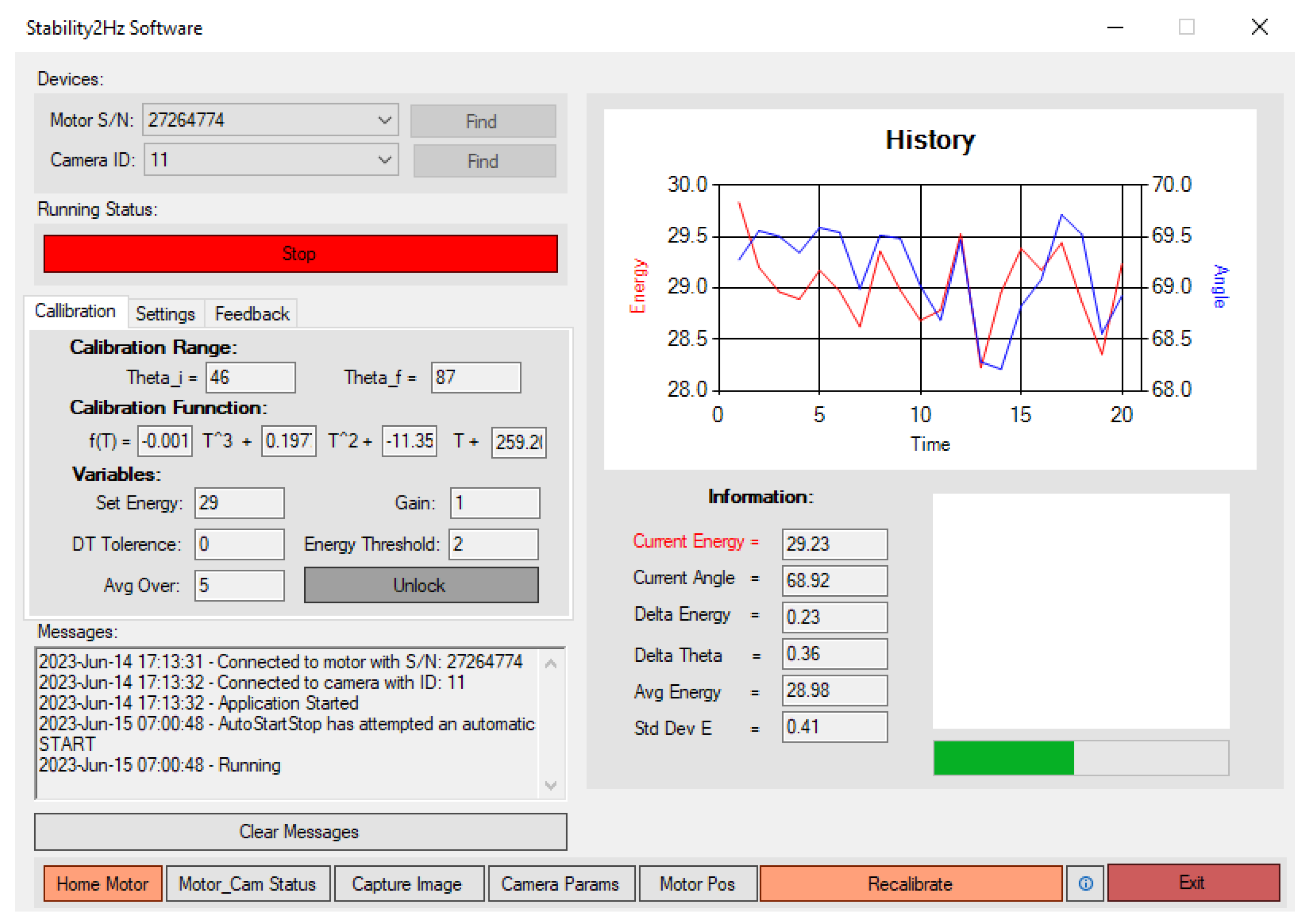
2.3. Software Development

The UI (Figure 5) was developed in NET Framework, primarily due to its built-in charting libraries. The application saves the last connected ThorLabs motor serial number and uEye camera ID to attempt an automatic connection next time the software is launched. An automatic run/stop functionality was added so that the code was not capturing images overnight when the laser was turned off, but was able to stabilise as soon as the laser was automatically turned on at the beginning of an operational day. This also allows the system to work within an operational environment without daily intervention from operators.

The user has control of all key parameters so that the functionality of the software can be optimised to the setup. The ‘set energy’ parameter is given in arbitrary units which correspond to those the camera gives intensity values in. We found a set energy of 29 camera units (316 mJ) to be optimal for operations. An ‘average over’ parameter reduces the systems ability to respond pulse-to-pulse, but increases its precision when responding to longer-term changes. The user can also choose to add a tolerance for delta theta, so that if the calculated change in angle is small, the WP is not commanded to move. The energy threshold parameter gives a minimum energy for the camera to detect for movement of the WP to occur. This should be set to be slightly greater than the maximum energy measurement when the laser is on and the waveplate–polariser is at minimum transmission, so that the WP is not commanded to go to its maximum when the laser is turned off, thus preventing excessive light from passing through the next time the laser is enabled. The history graph is useful for monitoring, as it displays the last m measurements, where m is the number of iterations, which the user can specify.

3. Analysis of Results

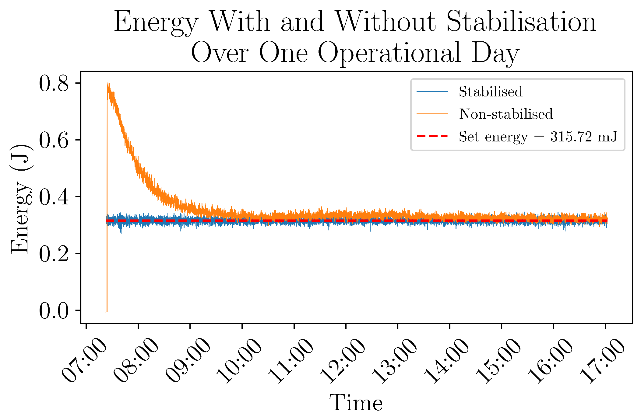
To assess the effectiveness of this method, we ran the system without active stabilization and for an entire day with active stabilization. In the first case, the software to measure the energy output with waveplate stabilisation was turned off. The second test ran for the same length of time, but with stabilisation running. The software was run as usual for operations on the day before testing, and the waveplate was then left at its final angle. It is then expected that if there is no drift or warm-up period, this angle being fixed would lead to a flat line in the energy reading with respect to time, i.e., the energy would be unchanging and equal to the energy measured at the end of the previous day, which was 29 energy units, or 316 mJ. On the day of the non-stabilising test, the laser was turned on at 7:00 a.m. but the internal shutter to the pump remained closed until 7:20 a.m.; this meant that no energy measurements could be captured during this time. This 20 min warm-up period was given to ensure that no internal damage to the system was caused, since it is expected that the energy would be far higher during these first few minutes. Figure 6 shows how the system has a higher energy at the start of the day, and gradually tailed off to the level of the set energy from the previous day. The period from the start to the point where we would consider using the laser without any stabilisation is around 2 h.

The system being operated with stabilisation shows limited improvement over the warmed-up oscillator energy between 10:00 a.m. (when the non-stabilised output energy had settled) and 17:00 p.m. (when the test was concluded). The standard deviations in this period for the non-stabilising and stabilising arrangements were ${\sigma }_{ns}=9.20$ mJ (2 d.p.) and ${\sigma }_s=8.85$ (2 d.p.), respectively. The intention of this system was never to improve the pulse-to-pulse stability, but only to minimise longer-term deviations, meaning this is not concerning. However, the mean energy for the stabilised system from 10:00 a.m. to 17:00 p.m. was ${\mu }_s=315.70$ (2 d.p.), when aiming for 315.72, whereas it was ${\mu }_{ns}=328.48$ mJ (2 d.p.) for the non-stabilised system over the same period. This shows that the stabilised system operates with a very high precision in the output, leading to operational benefits in energy predictability. All of this is summarised in Figure 6. The set energy (red dashed line) is added to show how good the two configurations are at reaching the set energy. We can see that in the non-stabilized case, the laser has an exponential decay to the reference energy over the first 2 h and it is visible that even afterwards there is a slow decay over almost the whole day to the reference energy.

4. Conclusions

Successful implementation of this system has decreased the laser warm-up time by 2–3 h, allowing the laser to be operational sooner. We have also proven the quadratic and then linear dependence of the energy on the camera pixel value, which is to be expected for a system based on p-n junctions. We have also proven a calibration mechanism that is iterative and could be applied to any high-energy solid-state laser system. The energy rms has also decreased to 2.8% from 3%.

The system also allows the energy output to be easily changed through software controls, and calibration ensures that the same energy can be achieved each day.

This technique could be easily replicated in any laser system encountering fluctuations in laser energy and long warm-up times.

References

- Zhao, B.; Banerjee, S.; Yan, W.; Zhang, P.; Zhang, J.; Golovin, G.; Liu, C.; Fruhling, C.; Haden, D.; Chen, S.; et al. Control over high peak-power laser light and laser-driven X-rays. Opt. Commun. 2018, 412, 141–145. [Google Scholar] [CrossRef]
- Parry, B.; Oliveira, P.; Boyle, A.; Shaikh, W.; Musgrave, I. A new ns opcpa front end for vulcan petawatt. CLF Annu. Rep. 2013, 2014. [Google Scholar]
- Hernandez-Gomez, C.; Collier, J.; Csatari, M.; Smith, J. Commissioning of the Vulcan OPCPA preamplifier. Annu. Rep. CLF Rutherford 2001, 175, 2001–2002. [Google Scholar]
- Ross, I.; Matousek, P.; Towrie, M.; Langley, A.; Collier, J. The prospects for ultrashort pulse duration and ultrahigh intensity using optical parametric chirped pulse amplifiers. Opt. Commun. 1997, 144, 125–133. [Google Scholar] [CrossRef]
- Dubietis, A.; Jonušauskas, G.; Piskarskas, A. Powerful femtosecond pulse generation by chirped and stretched pulse parametric amplification in BBO crystal. Opt. Commun. 1992, 88, 437–440. [Google Scholar] [CrossRef]
- Murari, K.; Cirmi, G.; Cankaya, H.; Stein, G.J.; Debord, B.; Gérôme, F.; Ritzkosky, F.; Benabid, F.; Muecke, O.; Kärtner, F.X. Sub-50 fs pulses at 2050 nm from a picosecond Ho:YLF laser using a two-stage Kagome-fiber-based compressor. Photon. Res. 2022, 10, 637–645. [Google Scholar] [CrossRef]
- Hubka, Z.; Antipenkov, R.; Boge, R.; Erdman, E.; Greco, M.; Green, J.T.; Horáček, M.; Majer, K.; Mazanec, T.; Mazůrek, P.; et al. 120 mJ, 1 kHz, picosecond laser at 515 nm. Opt. Lett. 2021, 46, 5655–5658. [Google Scholar] [CrossRef]
- Alexandridi, C.; Délen, X.; Druon, F.; Georges, P.; Martin, L.; Mathieu, F.; Papadopoulos, D. Generation of optically synchronized pump–signal beams for ultrafast OPCPA via the optical Kerr effect. Opt. Lett. 2021, 46, 2035–2038. [Google Scholar] [CrossRef]
- Seidel, M.; Pressacco, F.; Akcaalan, O.; Binhammer, T.; Darvill, J.; Ekanayake, N.; Frede, M.; Grosse-Wortmann, U.; Heber, M.; Heyl, C.M.; et al. Ultrafast MHz-Rate Burst-Mode Pump–Probe Laser for the FLASH FEL Facility Based on Nonlinear Compression of ps-Level Pulses from an Yb-Amplifier Chain. Laser Photonics Rev. 2022, 16, 2100268. [Google Scholar] [CrossRef]
- Haley, J.C.; Zheng, B.; Bertoli, U.S.; Dupuy, A.D.; Schoenung, J.M.; Lavernia, E.J. Working distance passive stability in laser directed energy deposition additive manufacturing. Mater. Des. 2019, 161, 86–94. [Google Scholar] [CrossRef]
- Maier, A.R.; Delbos, N.M.; Eichner, T.; Hübner, L.; Jalas, S.; Jeppe, L.; Jolly, S.W.; Kirchen, M.; Leroux, V.; Messner, P.; et al. Decoding Sources of Energy Variability in a Laser-Plasma Accelerator. Phys. Rev. X 2020, 10, 031039. [Google Scholar] [CrossRef]
- Abedin, K.M.; Al Jabri, A.R.; Mujibur Rahman, S. Power stability of different lasers and its effect on the outcome of phase-stepping shearography experiments. Results Opt. 2023, 12, 100490. [Google Scholar] [CrossRef]
- Ji, S.; Huang, W.; Guo, J.; Wang, J.; Lu, X.; Huang, D.; Wei, H.; Fan, W.; Li, X. Lamp-pumped eight-pass neodymium glass laser amplifier with high beam quality. Opt. Quantum Electron. 2021, 53, 277. [Google Scholar] [CrossRef]
- Zhu, J.; Zhu, J.; Li, X.; Zhu, B.; Ma, W.; Lu, X.; Fan, W.; Liu, Z.; Zhou, S.; Xu, G.; et al. Status and development of high-power laser facilities at the NLHPLP. High Power Laser Sci. Eng. 2018, 6, e55. [Google Scholar] [CrossRef]
Figure 1.
A schematic of the laser cavity. WP is the controllable waveplate, P1 and P2 are polarisers, PC is a Pockels’ cell, RGA is the regenerative amplifier, SHG is the second harmonic KDP crystal. The camera takes a Near-Field image on the penultimate mirror.
Figure 2.
Practical measurement of uEye camera’s calorimetry response using a Gentec MAESTRO energy detector. The extrapolated region is assumed as linear.
Figure 3.
The blue curve represents the original calibration function; the dashed blue curve represents the translated calibration function; current angle; calculated angle.
Figure 4.
A cubic calibration function (red) fit to measured energies from the camera as a function of angle.
Figure 5.
A capture of the UI of the Stability2 Hz software, developed in C#.
Figure 6.
The plot shows how the laser has a warm up period of around 2 h (orange trace). The blue curve sits at the same level as the set energy (red dashed line) for the duration of the day. Both plots have been converted to Joules using (1).
Disclaimer/Publisher’s Note: The statements, opinions and data contained in all publications are solely those of the individual author(s) and contributor(s) and not of MDPI and/or the editor(s). MDPI and/or the editor(s) disclaim responsibility for any injury to people or property resulting from any ideas, methods, instructions or products referred to in the content. |
© 2023 by the authors. Licensee MDPI, Basel, Switzerland. This article is an open access article distributed under the terms and conditions of the Creative Commons Attribution (CC BY) license (https://creativecommons.org/licenses/by/4.0/).
Share and Cite
MDPI and ACS Style
Morse, J.; Carter, W.; Oliveira, P.; Galimberti, M. Automated Long-Term Stability of a High-Energy Laser. Optics 2023, 4, 595-601. https://0-doi-org.brum.beds.ac.uk/10.3390/opt4040044
AMA Style
Morse J, Carter W, Oliveira P, Galimberti M. Automated Long-Term Stability of a High-Energy Laser. Optics. 2023; 4(4):595-601. https://0-doi-org.brum.beds.ac.uk/10.3390/opt4040044
Chicago/Turabian StyleMorse, Jack, William Carter, Pedro Oliveira, and Marco Galimberti. 2023. "Automated Long-Term Stability of a High-Energy Laser" Optics 4, no. 4: 595-601. https://0-doi-org.brum.beds.ac.uk/10.3390/opt4040044