Tunable, Nonmechanical, Fractional Talbot Illuminators

Abstract

Inside an optical Fourier processor, we inserted a varifocal system to continuously magnify the frequency of a master grating. The proposed system does not involve any mechanical compensation for scaling the Fourier spectrum. As the magnification, M, varies, the Fourier spectrum remains at the same initial location. We identified a previously unknown quadratic phase factor for generating, in the fixed output plane, Talbot images of any fractional order. We applied this result to setting a structured illumination beam, which does not have occluding regions. This illuminating beam can be useful for Talbot interferometry.

1. Introduction

At different ranges of the electromagnetic spectrum, as well as for matter waves, Talbot–Lau interferometers have found a myriad of useful applications. As a selected set of examples, we mention the following: X-ray nondestructive testing [1]; X-ray interferometry [2]; multi-contrast imaging [3]; neutron interference [4]; the space-time Talbot effect [5]; and the non-linear Talbot effect [6]. For an interesting review, see [7].

In the visible range, Talbot–Lau interferometers commonly employ a master grating that acts as a probe pattern. Then, in a Talbot image, one places a second grating for visualizing any local displacements, such as Moiré fringes [8].

For generating Moiré patterns with a tunable spatial frequency, it is desirable to scale the frequency of a master grating. To this end, several decades ago, Luxemoore proposed a simple technique for tuning the spatial frequency of the master grating [9]. In this technique, one illuminates the grating with a divergent beam, and one moves the grating along the optical axis.

Due to the finite, angular spread of the illuminating beam, this technique introduces variable vignetting. And, of course, the technique requires a mechanical device for implementing the desired axial displacements. In a heuristic description, Patorski proposed an extension of the Luxmoore technique for generating gratings with a tunable opening ratio [10].

Here, we note that in the latter two references, the descriptions ignore the presence of a quadratic phase factor, which is generated by the axial displacement. In what follows, we provide an analytical description that uses scalar diffraction in the paraxial regime. We show that, at a fixed plane, the quadratic phase factor is responsible for generating Talbot images of any fractional order. Next, we present the results of using a varifocal system to tune the frequency of the master grating without carrying out any mechanical interventions.

To achieve our aims, we exploited the remarkable advances in implementing varifocal lenses, providing methods free of any mechanical intervention. Some of these techniques include electrowetting [11,12,13,14], optofluidic variations [15,16,17,18,19], and the use of artificial muscles [20]. Here, the varifocal lenses continuously scale the frequency of the master grating. We recognize that the proposed device does not alter the location of the source [21,22].

Hence, in this study, our achievement is threefold. First, we present analytical formulas for describing controllable changes in scale of the virtual Fourier spectrum. Second, from our analytical formulations, we identified an unknown quadratic phase factor, which is responsible for generating Talbot images of arbitrary fractional orders. Third, we applied our formulations to designing a beam, which can illuminate a sample without occluding regions. This type of illumination beam is useful for Talbot interferometry.

In Section 2, we employ the concept of the virtual Fourier spectrum for identifying a scalable operation. In Section 3, we discuss the use of a varifocal system to continuously magnify, without any mechanical interventions, the spatial frequency of the master grating. In Section 4, we present the results of applying the frequency-scaling technique for scanning a sample, which was free of occluding regions. These results are useful for Talbot interferometry [23]. In Section 5, we summarize our contributions.

Here, we claim novelty with regard to three achievements: (a) we offer analytical descriptions of two techniques that control the spatial frequency of a master grating; (b) we unveil the use of two varifocal lenses for implementing a motionless method, which tunes the spatial frequency of a master grating; and (c) we propose a technique for generating a structural beam, which can illuminate a sample without occluding regions. This type of illumination can be useful for Talbot interferometry.

2. Tunable Spatial Frequency: Axial Displacements

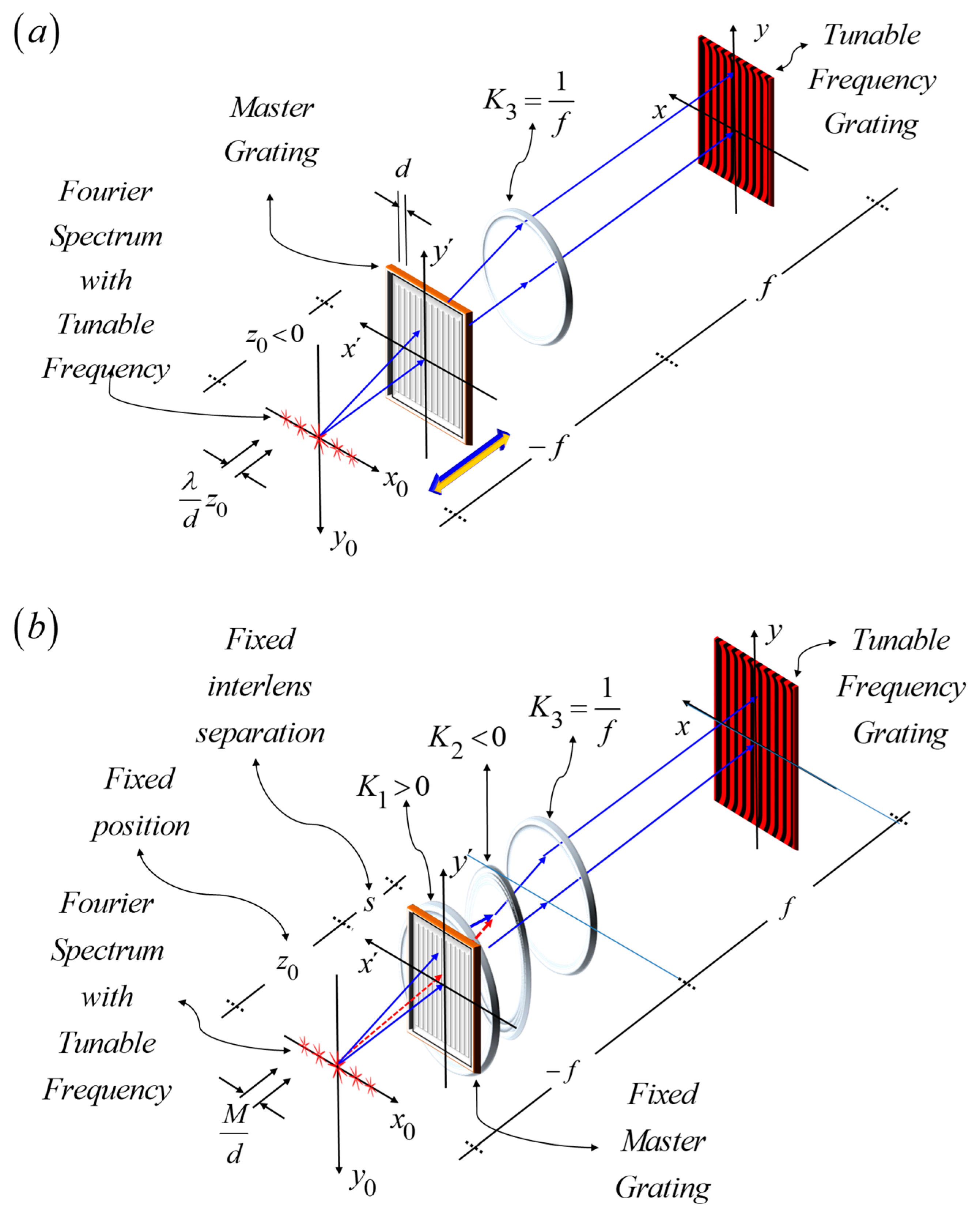
In Figure 1, we depict the optical setup under discussion. The master grating has a period equal to d. We denote the separation between the master grating and the illuminating point source as z₀. The separation z₀ was set as a negative number to facilitate our discussion in terms of geometrical optics.

One can observe, in Figure 1a, that the separation z₀ is variable for scaling the Fourier spectrum. To evade this motion, in Figure 1b, the separation z₀ is fixed. In our proposed apparatus, the axial motion of the master grating is substituted with the use of two varifocal lenses. These lenses magnify the Fourier spectrum without changing its axial position. In both cases, the position of the point source defines the input plane. In both setups, we employ a lens with a fixed optical power of K₃ = 1/f.

For our following discussion, the master grating is represented by its amplitude transmittance, which is expressed in terms of the Fourier series:

$$g\left(x^{\prime }\right)={\displaystyle \sum _{m\hspace{0.17em}=\hspace{0.17em}-\hspace{0.17em}\infty }^{\infty }}{C}_m\exp \left(i\hspace{0.17em}2\hspace{0.17em}\pi \hspace{0.17em}\frac{m}{d}{x}^{\prime }\right)$$

(1)

In Equation (1) the letter C_m denotes the Fourier coefficient of order m-th fold. The period of the grating is denoted as d. And trivially, the letter “m” stands for an integer number. Next, we identify the complex amplitude distribution of the spherical wave that comes from a point source, and it impinges on the master grating. Since z₀ < 0, the complex amplitude distribution is as follows:

$$\psi \left(x^{\prime };z_0\right)=\exp \left(\hspace{0.17em}i\hspace{0.17em}\pi \hspace{0.17em}\frac{{x^{\prime }}^2}{\lambda \hspace{0.17em}{z}_0}\right)\hspace{0.17em}g\left(x^{\prime }\right)$$

(2)

To obtain the complex amplitude distribution of the virtual Fourier spectrum, which is associated with Equation (2), we evaluate the following integral backwards with respect to the complex amplitude distribution at the source plane, the complex amplitude distribution is:

$$\psi \left(x_0;z_0\right)={\displaystyle \underset{-\hspace{0.17em}\infty }{\overset{\infty }{\int }}}\exp \left(-\hspace{0.17em}i\hspace{0.17em}\pi \hspace{0.17em}\frac{{\left(x_0-x^{\prime }\right)}^2}{\lambda \hspace{0.17em}{z}_0}\right)\hspace{0.17em}\hspace{0.17em}\hspace{0.17em}\psi \left(x^{\prime };z_0\right)\hspace{0.17em}\hspace{0.17em}d{x}^{\prime }.$$

(3)

If we substitute Equation (2) into Equation (3), we obtain

$$\psi \left(x_0;z_0\right)={\displaystyle \sum _{m\hspace{0.17em}=\hspace{0.17em}-\hspace{0.17em}\infty }^{\infty }}{C}_m\hspace{0.17em}\hspace{0.17em}\exp \left(\hspace{0.17em}-i\hspace{0.17em}2\hspace{0.17em}\pi \hspace{0.17em}\left(\frac{z_0}{Z_T}\right)\hspace{0.17em}{m}^2\right)\delta \left(x_0+\frac{\lambda \hspace{0.17em}{z}_0}{d}m\right)$$

(4)

In Equation (4), we employ the Talbot distance, which is

$$Z_T=2\frac{d^2}{\lambda }$$

(5)

In Equation (5) the Greek letter lambda stands for the wavelength of the monochromatic wave. As depicted in Figure 1a, the lens with fixed optical power optically implements the following Fourier transform:

$$q\left(x;z_0\right)={\displaystyle \underset{-\hspace{0.17em}\infty }{\overset{\infty }{\int }}}\psi \left(x_0;z_0\right)\hspace{0.17em}\hspace{0.17em}\exp \left(\hspace{0.17em}-i\hspace{0.17em}2\hspace{0.17em}\pi \hspace{0.17em}\frac{x}{\lambda f}{x}_0\right)\hspace{0.17em}\hspace{0.17em}d{x}_0$$

(6)

In Equation (6) the lower-case letter “f” denotes the focal length of the middle lens. If we substitute Equation (4) into Equation (5), we obtain the amplitude impulse response of the optical system:

$$q\left(x;z_0\right)={\displaystyle \sum _{m\hspace{0.17em}=\hspace{0.17em}-\hspace{0.17em}\infty }^{\infty }}{C}_m\hspace{0.17em}\hspace{0.17em}\exp \left(\hspace{0.17em}-i\hspace{0.17em}2\hspace{0.17em}\pi \hspace{0.17em}\left(\frac{z_0}{Z_T}\right)m^2\right)\exp \left(i\hspace{0.17em}2\hspace{0.17em}\pi \hspace{0.17em}m\left(\frac{z_0}{f\hspace{0.17em}d}\right)x\hspace{0.17em}\right)$$

(7)

In Equation (7), once again the upper-cas letter Z_T denotes the Talbot length. According to Equation (7), we can claim that the amplitude point spread function contains a non-previously identified quadratic phase factor, which is relevant for implementing a fractional Talbot image, by selecting the ratio z₀/Z_T. As expected, from Equation (7), it is apparent that the spatial frequency of the generated grating variation is

$$\frac{1}{d^{\prime }}=\left(\frac{z_0}{f}\right)\frac{1}{d}$$

(8)

To the best of our knowledge, the above formulation is novel. Hence, it is a contribution to the field of Talbot interferometry. In our previous discussion, we did not intend to argue in favor of the Luxmoore technique but rather to provide the necessary background for the following motionless method. However, before this, some practical considerations may be in order. The master grating can be a Ronchi ruling with an area of 50 (mm) × 50 (mm) and with 40 lines per millimeter. Then, the grating will have a total number of lines equal to two thousand. If the distance between the point source and the master grating is z₀ = −1 (m), the diffraction orders will be very slender areas. To fully illuminate this type of grating, the angular spread of the wave was set to about 3.2 degrees.

Next, we describe a novel, motionless method for controlling the spatial frequency, and for generating Talbot images of fractional order, in the same detection plane.

3. Tunable Frequency: Non-Mechanical Intervention

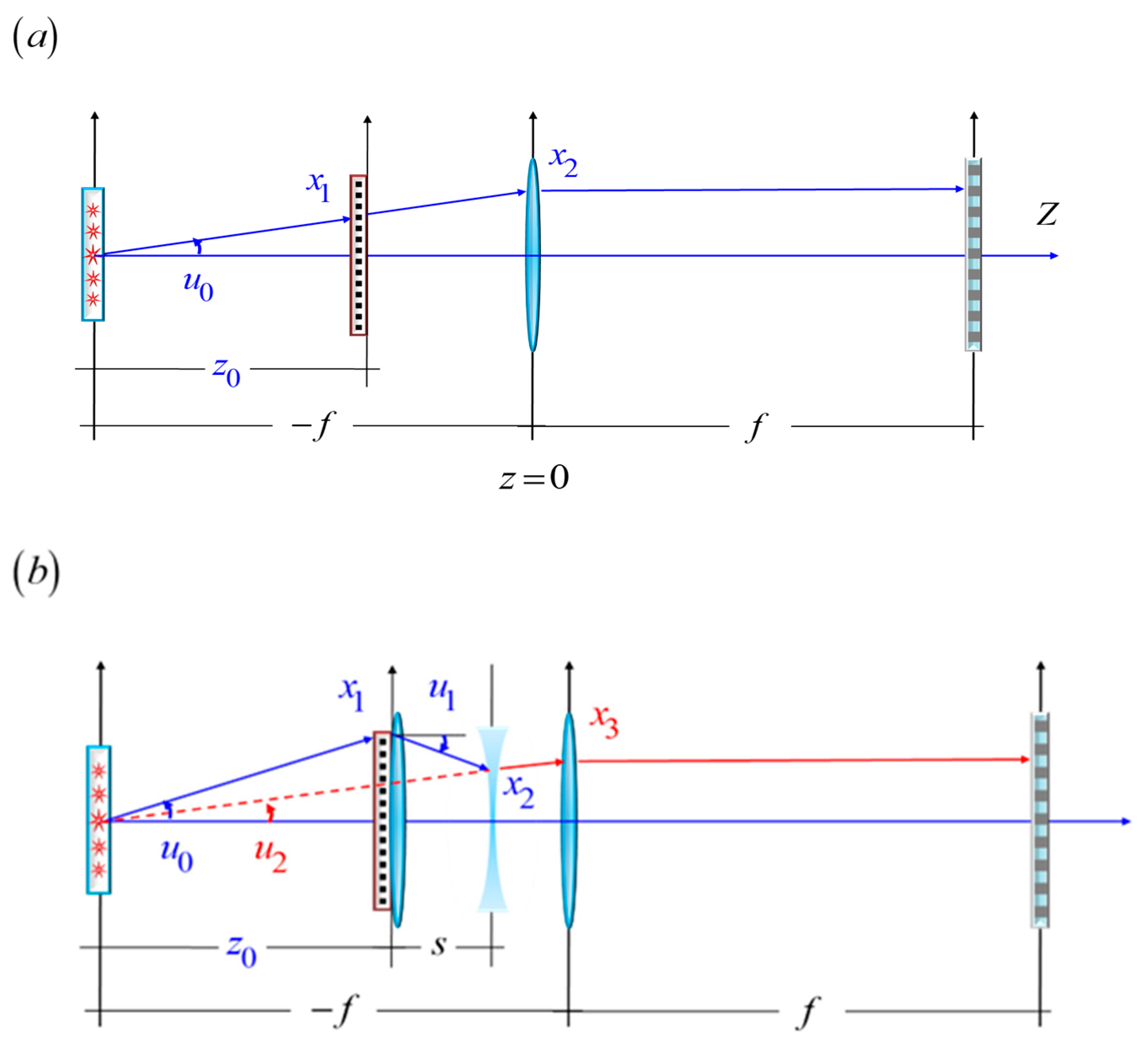
Here, we describe the use of a pair of varifocal lenses to obtain a motionless version of the previous result. Our discussion closely follows our previous results on geometrical optics [21,22]. In Figure 2, we show that the master grating is now fixed at the distance z₀. We place the first varifocal lens just after the master grating. Its optical power is equal to

$$K_1=\hspace{0.17em}\left(\frac{1}{s}\right)\left(1-\frac{s}{z_0}\right)\left(1-\frac{1}{M}\right)$$

(9)

In Equation (9), the lowercase letter “s” denotes the interlens separation between the first varifocal lens and a second element that is also varifocal. The uppercase letter “M” represents the tunable magnification. The second varifocal lens has the following optical power:

$$K_2=-\left(\frac{M-1}{s}\right)\left(\frac{1}{1-\frac{s}{z_0}}\right)$$

(10)

In Appendix A, we discuss the steps that we followed to obtain the optical powers in Equations (9) and (10).

By using the above varifocal lenses, one can reduce the exit angle by factor M; that is, u₂ = u₀/M. Consequently, one can laterally magnify the scale of the Fourier spectrum. In mathematical terms,

$$\psi \left(x_0;z_0\right)={\displaystyle \sum _{m\hspace{0.17em}=\hspace{0.17em}-\hspace{0.17em}\infty }^{\infty }}{C}_m\hspace{0.17em}\hspace{0.17em}\exp \left(\hspace{0.17em}-i\hspace{0.17em}2\hspace{0.17em}\pi \hspace{0.17em}{M}^2\left(\frac{z_0}{Z_T}\right)\hspace{0.17em}{m}^2\right)\delta \left(x_0+M\frac{\lambda \hspace{0.17em}{z}_0}{d}m\right)$$

(11)

Again, the third lens, with a fixed optical power, implements a Fourier transformation of Equation (11); in this way, we obtain the new complex amplitude response:

$$q\left(x;z_0\right)={\displaystyle \sum _{m\hspace{0.17em}=\hspace{0.17em}-\hspace{0.17em}\infty }^{\infty }}{C}_m\hspace{0.17em}\hspace{0.17em}\exp \left(\hspace{0.17em}-i\hspace{0.17em}2\hspace{0.17em}\pi \hspace{0.17em}{M}^2\hspace{0.17em}\left(\frac{z_0}{Z_T}\right)m^2\right)\exp \left(i\hspace{0.17em}2\hspace{0.17em}\pi \hspace{0.17em}m\left(\frac{M\hspace{0.17em}{z}_0}{f\hspace{0.17em}d}\right)x\hspace{0.17em}\right)$$

(12)

As we defined previously, the upper-case letter M denotes the variable magnification. The lower-case letter “f” stands for the focal length of the central lens. And the lower-case letter “d” is the period of the master grating. It is apparent from Equation (12) that for a fixed value of z₀, the proposed optical system can modify the quadratic phase factor, which is responsible for obtaining fractional Talbot images. In other words, let us assume that z₀ = Z_T/L, where L is a positive integer number. Then, Equation (12) assumes the following form:

$$q\left(x;z_0\right)={\displaystyle \sum _{m\hspace{0.17em}=\hspace{0.17em}-\hspace{0.17em}\infty }^{\infty }}{C}_m\hspace{0.17em}\hspace{0.17em}\exp \left(\hspace{0.17em}-i\hspace{0.17em}2\hspace{0.17em}\pi \hspace{0.17em}\left(\frac{M^2}{L}\right)m^2\right)\exp \left(i\hspace{0.17em}2\hspace{0.17em}\pi \hspace{0.17em}\left(\frac{m}{d^{\prime }}\right)\hspace{0.17em}x\hspace{0.17em}\right)$$

(13)

In Equation (13), we are employing our previous notation for the variables in play. And we note that the generated grating has a tunable spatial frequency:

$$\frac{1}{d^{\prime }}=\left(\frac{2M}{L}\right)\left(\frac{d}{\lambda \hspace{0.17em}f}\right)$$

(14)

Once the value of L has been chosen, in the same detection plane, one can attain a fractional Talbot image of any order between 1/L and unity by setting the magnification in the interval as follows:

$$1\le M\le \sqrt{L}$$

(15)

Based on these results, we can claim that in the same detection plane, one can generate tunable gratings that are fractional Talbot images. To the best of our knowledge, the above formulation is novel. Hence, it is a contribution to the field of Talbot interferometry. Next, we apply these results.

4. Talbot Illuminator of Variable Fractional Orders

For the following application, it is convenient to discuss the generation of fractional Talbot images, serving as a linear combination of laterally displaced versions of the initial grating. Since this approach is not very well known, in Appendix B, we discuss the details of this description. Here, it suffices to note that the amplitude impulse response, shown in Equation (7), can be written as follows:

$$q\left(x;z_0\right)={\displaystyle \sum _{n\hspace{0.17em}=\hspace{0.17em}0\hspace{0.17em}}^{N-1}}{W}_n\left(z_0\right)\hspace{0.17em}\hspace{0.17em}g\left(x-\frac{n}{N}d\right)$$

(16)

In Equation (16) we denote as W_n (z₀) the weighting factors (or if you will the coefficients) of the linear expansion. The coefficients in the linear combination were obtained by evaluating the following discrete Fourier transform:

$$W_n\left(z_0\right)=\frac{1}{N}{\displaystyle \sum _{m\hspace{0.17em}=\hspace{0.17em}0\hspace{0.17em}}^{N-1}}\exp \left(\hspace{0.17em}-i\hspace{0.17em}2\hspace{0.17em}\pi \hspace{0.17em}\left(\frac{z_0}{Z_T}\right)m^2\right)\hspace{0.17em}\exp \left(\hspace{0.17em}i\hspace{0.17em}2\hspace{0.17em}\pi \frac{n\hspace{0.17em}m}{N}\right)$$

(17)

To illustrate the use of this approach, next, we evaluate the simple case of N = 2. Other cases are beyond our current scope. Let us assume that the master grating is a binary grating with a duty cycle equal to one half. Then, its amplitude transmittance is

$$g\left(x\right)=rect\left(\frac{2\hspace{0.17em}x}{d}\right)\ast {\displaystyle \sum _{m\hspace{0.17em}=\hspace{0.17em}-\hspace{0.17em}\infty }^{\infty }}\delta \left(x-m\hspace{0.17em}d\right)$$

(18)

In Equation (18) the starisk denoted the convolution operation. And the Greek letter delta represents a Dirac’s delta. Futhermore, in Equation (18), we use the common notation of a rectangular function to represent the amplitude transmittance of the unit cell. According to our current description, the Fresnel diffraction patterns can be described as a linear superposition of the initial grating g(x) and the complementary transmittance g(x − d/2). It is clear from the definition in Equation (12) that the complex amplitude factors for g(x) and g(x − d/2) are

$$W_0\left(z_0\right)=\exp \left(\hspace{0.17em}-i\hspace{0.17em}\pi \hspace{0.17em}\left(\frac{z_0}{Z_T}\right)m^2\right)\hspace{0.17em}\hspace{0.17em}\hspace{0.17em}\cos \hspace{0.17em}\left(\pi \left(\frac{z_0}{Z_T}\right)\right).$$

(19)

$$W_1\left(z_0\right)=i\hspace{0.17em}\hspace{0.17em}\exp \left(\hspace{0.17em}-i\hspace{0.17em}\pi \hspace{0.17em}\left(\frac{z_0}{Z_T}\right)m^2\right)\hspace{0.17em}\hspace{0.17em}\hspace{0.17em}\sin \hspace{0.17em}\left(\pi \frac{z_0}{Z_T}\right).$$

(20)

Hence, the complex amplitude point spread function can be written as follows:

$$q\left(x;z_0\right)=\exp \left(\hspace{0.17em}-i\hspace{0.17em}\pi \hspace{0.17em}\left(\frac{z_0}{Z_T}\right)m^2\right)\hspace{0.17em}\hspace{0.17em}\left[\cos \hspace{0.17em}\left(\pi \left(\frac{z_0}{Z_T}\right)\right)\hspace{0.17em}g\left(x\right)+i\hspace{0.17em}\sin \hspace{0.17em}\left(\pi \left(\frac{z_0}{Z_T}\right)\right)g\left(x-\frac{d}{2}\right)\right]$$

(21)

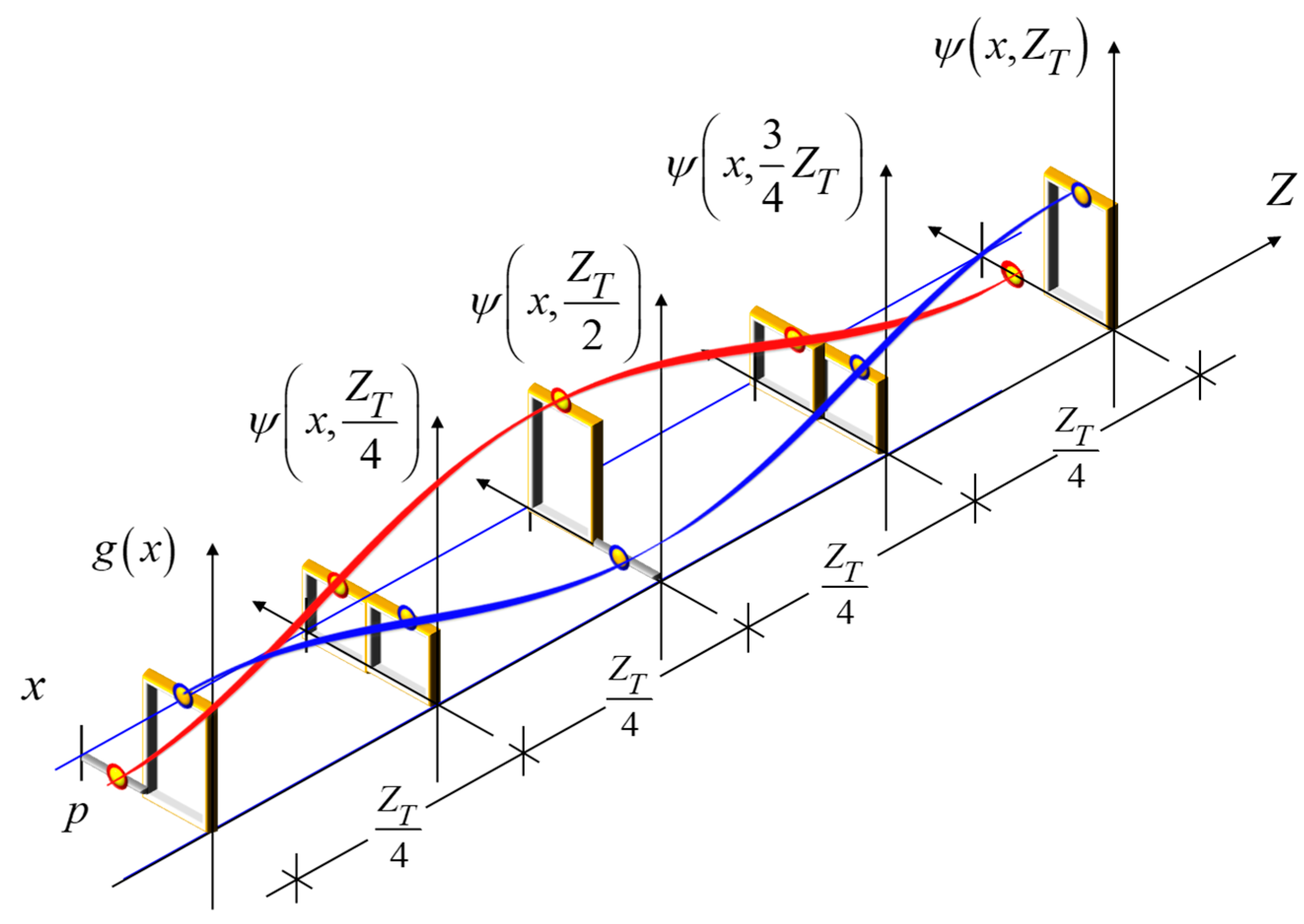
To the best of our knowledge, Equations (19)–(21) have not been presented before. Hence, they are contributions to the field of Talbot interferometry. In Figure 3, we represent the sinusoidal variations of these coefficients at planes located at multiple values of one quarter of the Talbot length. In blue, the sinusoidal variations depict the coefficient in Equation (12). And, in red, the curve describes the variations in Equation (13).

And, consequently, the irradiance distribution is as follows:

$$\hspace{0.17em}\hspace{0.17em}I\left(x,z\right)={\left|g\left(x\right)\right|}^2\hspace{0.17em}{\cos }^2\left(\pi \left(\frac{z_0}{Z_T}\right)\right)+{\left|g\left(x-\frac{d}{2}\right)\right|}^2{\sin }^2\left(\pi \left(\frac{z_0}{Z_T}\right)\right)\hspace{0.17em}$$

(22)

In Equation (22) we are employing the common notation of the square modulus, of the master grating. By setting z₀ = Z_T/4, the initial coefficients W₀ and W₁ assume the same values. Therefore, in these planes, the fractional Talbot images generate a uniform irradiance distribution. However, as expressed in Equation (14), the complex amplitude distribution is not uniform. In fact, the complex amplitude distribution is that of a phase grating, which resembles a structured illumination with non-occluding regions. Then, we claim that the periodic complex amplitude distribution can be used for coding a sample, without incurring occluding regions.

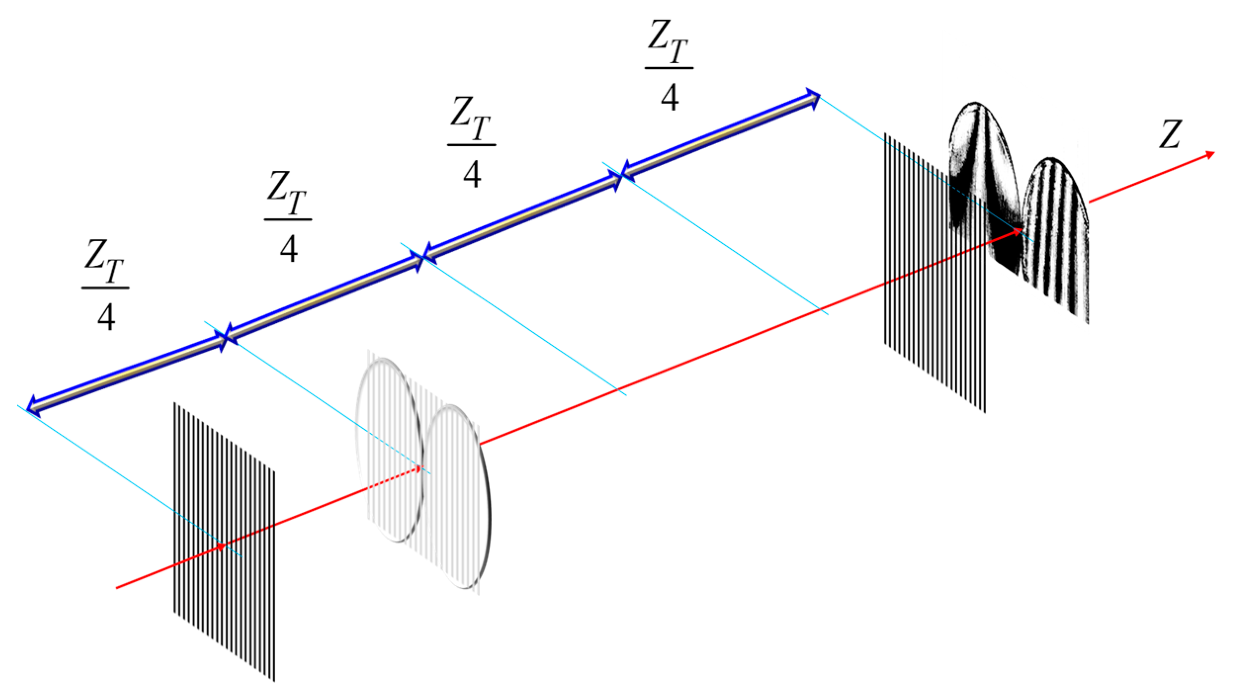
In Figure 4, we depict the proposed technique.

In Figure 4, the amplitude transmittance of the generated grating is that expressed in Equation (18). As is indicated in Equation (22), at one quarter of the generated grating there lies a transparent structure. A pair of phase samples are located in this plane. The samples modify the illuminating structure. At the Talbot distance, a second grating is used to visualize, as Moiré patterns, the modified grating.

5. Conclusions

To continuously change the spatial frequency of a master grating, we have revisited the Luxmoore technique. Herein, we have presented the first analytical description of this technique. To achieve this first goal, we used the concept of the virtual Fourier spectrum. Based on our analytical description, we identified an unknown quadratic phase factor. We have indicated that this quadratic phase is useful for obtaining, at a fixed plane, an arbitrary fractional-order Talbot image.

As a second contribution, we presented a motionless technique for continuously varying the spatial frequency of a master grating. To achieve this, we used a pair of varifocal lenses that magnify the Fourier spectrum of the master grating. As the magnification changes, the Fourier spectrum remains in its initial fixed position. We have unveiled an analytical formula for obtaining the variable spatial frequency.

As a third contribution, we noted that by using our motionless technique, one can use the controllable magnification to set a fractional Talbot image in a fixed plane. This novel property was used to generate a structured beam in order to illuminate a sample without occluding regions. This type of illumination can be useful for Talbot interferometry.

References

- Morimoto, N.; Shirai, T.; Kimura, K.; Doki, T.; Sano, S.; Horiba, A.; Kitamura, K. Talbot–Lau interferometry-based X-ray imaging system, with retractable and rotatable gratings for nondestructive testing. Rev. Sci. Instrum. 2020, 91, 023706. [Google Scholar] [CrossRef]
- Bouffetier, V.; Ceurvorst, L.; Valdivia, M.P.; Dorchies, F.; Hulin, S.; Goudal, T.; Stutman, D.; Casner, A. Proof-of-concept Talbot–Lau X-ray interferometry with a high-intensity, high repetition-rate, laser-driven K-alpha source. Appl. Opt. 2020, 59, 8380–8387. [Google Scholar] [CrossRef] [PubMed]
- Deng, K.; Li, J.; Xie, W. Modeling the Moiré fringe visibility of Talbot-Lau X-ray grating interferometry for single-frame multi-contrast imaging. Opt. Express 2020, 28, 27107–27122. [Google Scholar] [CrossRef] [PubMed]
- Neuwirth, T.; Backs, A.; Gustschin, A.; Vogt, S.; Pfeiffer, F.; Böni, P.; Schulz1, M. A high visibility Talbot-Lau neutron grating interferometer to investigate stress-induced magnetic degradation in electrical steel. Nat. Sci. Rep. 2020, 10, 1764. [Google Scholar] [CrossRef] [PubMed]
- Hall, L.A.; Yessenov, M.; Sergey, A.; Ponomarenko, S.A.; Abouraddy, A.F. The space–time Talbot effect. Appl. Phys. Lett. Photon. 2021, 6, 056105. [Google Scholar] [CrossRef]
- Yang, Z. Nonlinear Talbot Effect and Its Applications. IOP Conf. Ser. Earth Environ. Sci. 2018, 128, 012047. [Google Scholar] [CrossRef]
- Wen, J.; Zhang, Y.; Xiao, M.M. The Talbot effect: Recent advances in classical optics, nonlinear optics, and quantum optics. Adv. Opt. Photon. 2013, 5, 3–130. [Google Scholar] [CrossRef]
- Lohmann, A.W.; Silva, D.E. An interferometer based on the Talbot effect. Opt. Commun. 1971, 2, 413–415. [Google Scholar] [CrossRef]
- Luxmoore, A. Optical projection system for the Moiré method of surface strain measurement. In Optical Instruments and Techniques; Dickson, J.H., Ed.; Oriel Press: London, UK, 1971; p. 200. [Google Scholar]
- Patorski, K. Production of binary amplitude gratings with arbitrary opening ratio and variable period. Opt. Laser Technol. 1980, 12, 267–270. [Google Scholar] [CrossRef]
- Lee, J.; Lee, J.; Won, Y.H. Nonmechanical three-dimensional beam steering using electrowetting-based liquid lens and liquid prism. Opt. Express 2019, 27, 36757–36766. [Google Scholar] [CrossRef]
- Lia, J.; Kim, C.-J. Current commercialization status of electrowetting-on-dielectric (EWOD) digital microfluidics. Lab A Chip 2019, 20, 1705–1712. [Google Scholar] [CrossRef]
- Song, X.; Zhang, H.; Li, D.; Jia, D.; Liu, T. Electrowetting lens with large aperture and focal length tunability. Sci. Rep. 2020, 10, 16318. [Google Scholar] [CrossRef]
- Wang, D.; Hu, D.; Zhou, Y.; Sun, L. Design and fabrication of a focus-tunable liquid cylindrical lens based on electrowetting. Opt. Express 2022, 30, 47430–47439. [Google Scholar] [CrossRef]
- Chen, Q.; Li, T.; Li, Z.; Long, J.; Zhang, X. Optofluidic Tunable Lenses for In-Plane Light Manipulation. Micromachines 2018, 9, 97. [Google Scholar] [CrossRef]
- Ciraulo, B.; Garcia-Guirado, J.; de Miguel, I.; Ortega-Arroyo, J.; Quidant, R. Long-range optofluidic control with plasmon heating. Nat. Commun. 2021, 12, 2001. [Google Scholar] [CrossRef] [PubMed]
- Lee, J.; Park, Y.; Chung, S.K. Multifunctional liquid lens for variable focus and aperture. Sens. Actuators A Phys. 2019, 425, 177–184. [Google Scholar] [CrossRef]
- Fang, Y.-C.; Tzeng, Y.-F.; Wen, C.-C.; Chen, C.-H.; Lee, H.-Y.; Chang, S.-H.; Su, Y.-L. A Study of High-Efficiency Laser Headlight Design Using Gradient-Index Lens and Liquid Lens. Appl. Sci. 2020, 10, 7331. [Google Scholar] [CrossRef]
- Liu, C.; Wang, D.; Wang, Q.-H.; Xing, Y. Multifunctional optofluidic lens with beam steering. Opt. Express 2020, 28, 7734–7745. [Google Scholar] [CrossRef] [PubMed]
- Wang, Y.; Ma, X.; Jiang, Y.; Zang, W.; Cao, P.; Tian, M.; Ning, N.; Zhang, L. Dielectric elastomer actuators for artificial muscles: A comprehensive review of soft robot explorations. Resour. Chem. Mater. 2020, 1, 308–324. [Google Scholar] [CrossRef]
- Gómez-Sarabia, C.M.; Ojeda- Castañeda, J. Hopkins procedure for tunable magnification: Surgical spectacles. Appl. Opt. 2020, 59, D59–D63. [Google Scholar] [CrossRef]
- Gómez-Sarabia, C.M.; Ojeda- Castañeda, J. Two-conjugate zoom system: The zero-throw advantage. Appl. Opt. 2020, 59, 7099–7102. [Google Scholar] [CrossRef] [PubMed]
- Ojeda-Castañeda, J. Wavefront Shaping, and Pupil Engineering; Springer: Berlin/Heidelberg, Germany, 2021. [Google Scholar]
Figure 1.
Schematics of the optical setups for varying the spatial frequency of a master grating. (a) The arrangement described by Luxmoore. In this arrangement, the master grating moves along the optical axis to scale its Fourier spectrum, and a fixed optical power lens implements a Fourier transform of the scaled Fourier spectrum. (b) Our proposed apparatus. Instead of moving the master grating, two varifocal lenses magnify the Fourier spectrum, which remains in a fixed axial position.
Figure 2.
Schematics of the ray optics description of the optical system. (a) For comparison, the optical setup proposed by Luxmoore. (b) The optical setup that incorporates two varifocal lenses.
Figure 3.
Complex amplitude distribution, at various fractions of the Talbot length, associated with an initial binary grating with a duty cycle (fill factor) equal to one half of the period. The complex amplitude variations of the unit cell are shown in blue. The complex amplitude variations of the complementary cell are shown in red.
Figure 4.
Not-to-scale picture showing the irradiance distribution at the Talbot length of the master grating. We assume that the sample is illuminated with the complex amplitude in Equation (14). For the sake of clarity, in this picture, the detecting grating is placed slightly before the detecting plane.
Disclaimer/Publisher’s Note: The statements, opinions and data contained in all publications are solely those of the individual author(s) and contributor(s) and not of MDPI and/or the editor(s). MDPI and/or the editor(s) disclaim responsibility for any injury to people or property resulting from any ideas, methods, instructions or products referred to in the content. |
© 2023 by the authors. Licensee MDPI, Basel, Switzerland. This article is an open access article distributed under the terms and conditions of the Creative Commons Attribution (CC BY) license (https://creativecommons.org/licenses/by/4.0/).
Share and Cite
MDPI and ACS Style
Gómez-Sarabia, C.M.; Ojeda-Castañeda, J. Tunable, Nonmechanical, Fractional Talbot Illuminators. Optics 2023, 4, 602-612. https://0-doi-org.brum.beds.ac.uk/10.3390/opt4040045
AMA Style
Gómez-Sarabia CM, Ojeda-Castañeda J. Tunable, Nonmechanical, Fractional Talbot Illuminators. Optics. 2023; 4(4):602-612. https://0-doi-org.brum.beds.ac.uk/10.3390/opt4040045
Chicago/Turabian StyleGómez-Sarabia, Cristina M., and Jorge Ojeda-Castañeda. 2023. "Tunable, Nonmechanical, Fractional Talbot Illuminators" Optics 4, no. 4: 602-612. https://0-doi-org.brum.beds.ac.uk/10.3390/opt4040045