On the Accuracy of the Sine Power Lomax Model for Data Fitting

Abstract

Every day, new data must be analysed as well as possible in all areas of applied science, which requires the development of attractive statistical models, that is to say adapted to the context, easy to use and efficient. In this article, we innovate in this direction by proposing a new statistical model based on the functionalities of the sinusoidal transformation and power Lomax distribution. We thus introduce a new three-parameter survival distribution called sine power Lomax distribution. In a first approach, we present it theoretically and provide some of its significant properties. Then the practicality, utility and flexibility of the sine power Lomax model are demonstrated through a comprehensive simulation study, and the analysis of nine real datasets mainly from medicine and engineering. Based on relevant goodness of fit criteria, it is shown that the sine power Lomax model has a better fit to some of the existing Lomax-like distributions.

1. Introduction

A large part of applied mathematics consists of defining one or more models of a mathematical nature, allowing a sufficiently general consideration of a given phenomenon. In a somewhat schematic way, we can distinguish two kinds of modelling: the deterministic modelling where random variations are not taken into account and stochastic modelling which takes into account these random variations (roughly speaking, ‘stochastic’ means to be or have a random variable). In the context of stochastic modelling, the random variations are often associated with an underlying probability distribution. Stochastic modelling can be divided into two sub-categories: probabilistic modelling and statistical modelling. The main objective of the probabilistic modelling is to provide a formal framework making it possible to describe the random variations discussed above, and to study the general properties of the phenomena which govern them. More applied, the statistical modelling essentially consists of defining suitable tools aiming to model the observed data taking into account their random nature. This theme is fully developed in [1,2], among others.

Recent developments in stochastic modelling have been driven by the rapid progress and accessibility of computing power. In particular, these have allowed direct applications of existing continuous distributions with some functional complexity for various statistical purposes. Also, these have accelerated the creation of new families of distributions presenting original and practical characteristics. In this regard, we may refer to [3] for a complete overview. Among the latest developments, the families defined by ‘trigonometric transformations’ of a given distribution have attracted much attention due to their applicability and working capacity in many practical situations. The pioneering works of [4,5,6,7] have focused on the sinusoidal transformation leading to the so-called sine generated (S-G or Sin-G) family. The following equations are the generic definitions of the associated cumulative distribution function (cdf) and probability density function (pdf), respectively:

$$F_S(x;\zeta )=sin\left[\frac{\pi }{2}G(x;\zeta )\right],x\in \mathbb{R}$$

(1)

and

$$f_S(x;\zeta )=\frac{\pi }{2}g(x;\zeta )cos\left[\frac{\pi }{2}G(x;\zeta )\right],x\in \mathbb{R}.$$

(2)

In these equations, $G(x;\zeta )$ and $g(x;\zeta )$ are the cdf and pdf of a certain continuous distribution with parameter(s) vector denoted by $\zeta$, respectively. They are related to a reference distribution chosen a priori by the practitioner, depending on the context of the study. It is now established that the S-G family (i) offers an attractive alternative to the reference family; one can show that $G(x;\zeta )\le F_S(x;\zeta )$ for any $x\in \mathbb{R}$, (ii) is of acceptable mathematical complexity without introducing new parameters, and (iii) has the ability to provide flexible statistical models to accommodate data of varying nature. To illustrate these items, in Reference [4], the exponential distribution is used as a reference to define the SE model. It turns out to be well suited to analyse the important bladder cancer patients dataset of [8]. In another study, the inverse Weibull (IW) distribution developed by [9] was considered to be the reference distribution; the sine IW (SIW) model was introduced by [6]. By analyzing the famous guinea pigs dataset by [10], the SIW model is proven to perform better compared to serious and comparable competing models. An open-source R package on the SIW model is developed in [11], facilitating the use of the model beyond these basic purposes. These works inspired the construction of other trigonometric families of distributions, such as the CS-G family by [12], C-G family by [7], TransSC-G family by [13], NS-G family by [14], STL-G family by [15] and SKum-G family by [16].

In this paper, we contribute to the success of the S-G family by applying it to a specific three-parameter survival distribution: the power Lomax (PL) distribution proposed by [17]. We thus introduce the sine PL (SPL) distribution and model. Thus, a retrospective on the PL distribution is necessary to understand the proposed methodology. First, the Lomax distribution was introduced by [18]. It can be presented as a manageable two-parameter heavy-tailed survival distribution with a tuning polynomial decay and also, as a derivation of the Pareto distribution as described in [19] (page 573). It is governed by the cdf and pdf defined by

$$G_L(x;\xi )=1-{\left(1+\lambda x\right)}^{-\alpha },x>0$$

(3)

and

$$g_L(x;\xi )=\alpha \lambda {(1+\lambda x)}^{-(\alpha +1)},x>0,$$

(4)

respectively, with $G_L(x;\xi )=g_L(x;\xi )=0$ for $x\le 0$, where $\xi =(\alpha ,\lambda )$, $\alpha$ is a shape parameter and $\lambda$ is a scale parameter, all the parameters taking strictly positive values. It finds numerous applications in reliability engineering and life testing. The theory, inference and applications of the Lomax distribution have been the subjects of the following inevitable references: [20,21,22,23,24,25,26]. The PL distribution proposed by [17] is obtained by making use of the power transformation to the Lomax distribution, aiming to increase its capabilities on several functional aspects. It corresponds to the distribution of the random variable $X=Y^{1/\beta }$, where Y is a random variable with the Lomax distribution and $\beta >0$. Consequently, based on (3) and (4), the PL distribution is defined by the cdf and pdf defined by

$$G_{PL}(x;\zeta )=G_L(x^{\beta };\xi )=1-{\left(1+\lambda x^{\beta }\right)}^{-\alpha },x>0$$

(5)

and

$$g_{PL}(x;\zeta )=\alpha \beta \lambda x^{\beta -1}{\left(1+\lambda x^{\beta }\right)}^{-(\alpha +1)},x>0,$$

(6)

respectively, with $G_{PL}(x;\zeta )=g_{PL}(x;\zeta )=0$ for $x\le 0$, where $\zeta =(\alpha ,\beta ,\lambda )$, $\alpha$ is a shape parameter, and $\beta$ and $\lambda$ are scale parameters, all the parameters taking strictly positive values. Contrary to the Lomax distribution, it is established in [17] that the PL distribution adapts to both inverted bathtub and decreasing hazard rates. The practical gain is particularly impressive; the PL model is better than ten competing models for analyzing the bladder cancer patients dataset of [8], all based on the Lomax model. For the sake of optimality, some motivated distributions extending or generalizing the PL distribution was introduced, including the type II Topp-Leone PL (TIITLPL) distribution by [27], type I half logistic PL distribution by [28], inverse PL distribution by [29], Marshall-Olkin PL distribution by [30], exponentiated PL distribution by [31] and Kumaraswamy generalized PL distribution (KPL) by [32]. The main strategy of these proposed distributions is to add more parameters to the PL distribution based on exponentiated, transmuted or truncated schemes. Basically, these schemes give better results but add more parameters to the reference distribution; the problem of manipulating all these parameters simultaneously can present a certain difficulty from the modelling point of view. Thus, the immediate motivation of the SPL model is to use the S-G scheme to improve the efficiency of the PL model with the existing parameters. Deeper motivations come after further investigation which is detailed in the next study. To summarize, the functionality and flexibility of the SPL model are particularly attractive for data fitting. Indeed, the corresponding pdf has different kinds of curves such as uni-modal, symmetrical, asymmetrical on right and left, reversed J-shaped curves. Also, the model exhibits decreasing and increasing, inverted bathtub and reversed-J hazard rates. These properties give the SPL model a constant consistency in the precision of the fits unlike many other comparable models. This statement is illustrated in the practical environment by considering nine published datasets mainly from medicine and engineering, and four competing models derived from the Lomax distribution.

We organize the rest of the paper as follows. Section 2 is devoted to the definition, characteristics and main properties of the SPL distribution. The parametric estimation related to the SPL model is discussed and illustrated by a comprehensive simulation study in Section 3. Concrete applications to datasets are provided in Section 4. Finally, conclusions are stated in Section 5.

2. The SPL Distribution

2.1. Function Anlysis

Here, some mathematics of the SPL distribution are presented. First, by considering (5) and (6) in (1) and (2), we obtain the main distributional functions of the SPL distribution; the corresponding cdf and pdf are given as

$$F_{SPL}(x;\zeta )=cos\left(\frac{\pi }{2}{(1+\lambda x^{\beta })}^{-\alpha }\right),x>0$$

(7)

where $\zeta =(\alpha ,\beta ,\lambda )$, and

$$f_{SPL}(x;\zeta )=\frac{\pi }{2}\alpha \beta \lambda x^{\beta -1}{(1+\lambda x^{\beta })}^{-(\alpha +1)}sin\left(\frac{\pi }{2}{(1+\lambda x^{\beta })}^{-\alpha }\right),x>0,$$

(8)

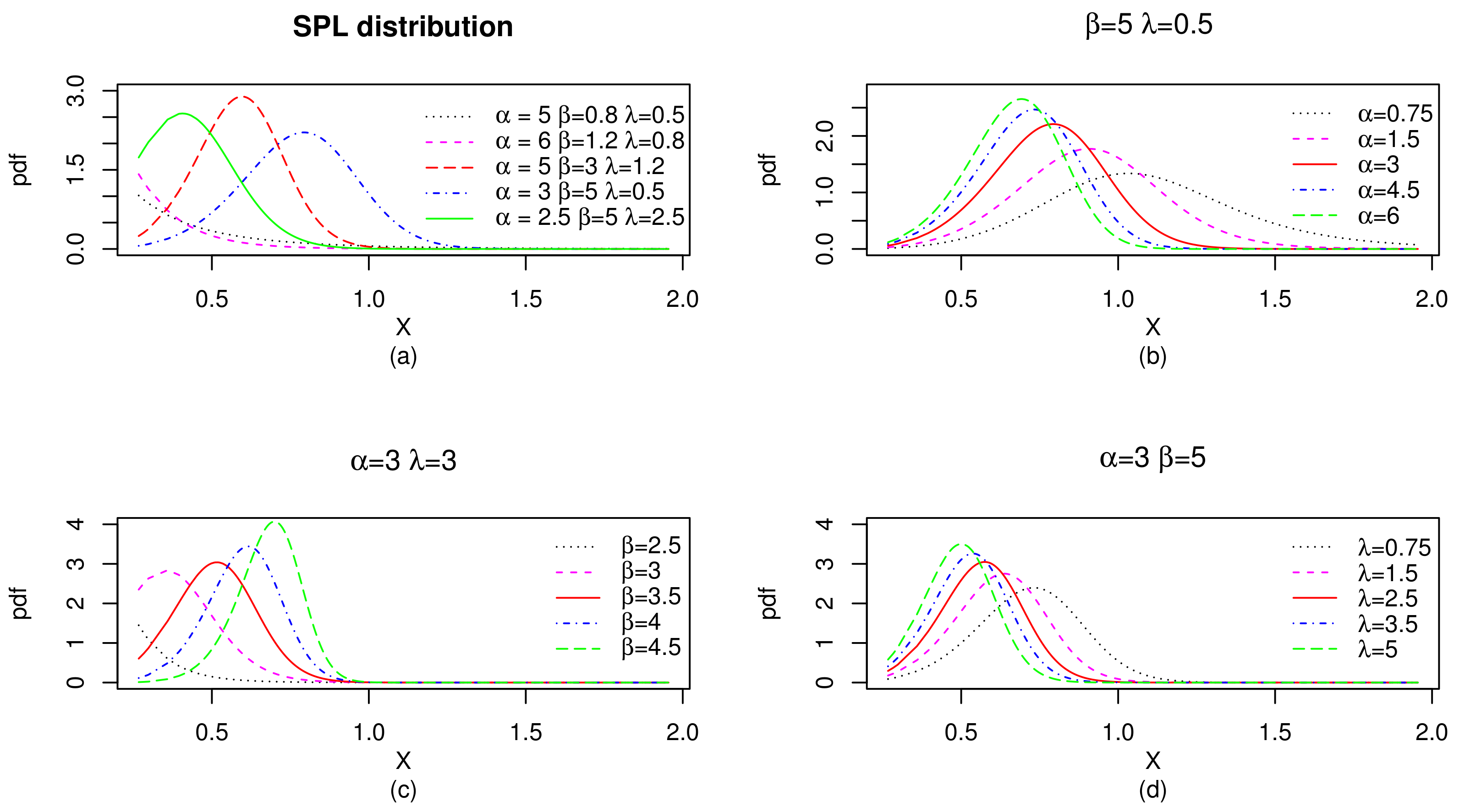
with $F_{SPL}(x;\zeta )=f_{SPL}(x;\zeta )=0$ for $x\le 0$. We recall that $\zeta =(\alpha ,\beta ,\lambda )$, $\alpha$ is a shape parameter, and $\beta$ and $\lambda$ are scale parameters, all the parameters taking strictly positive values. Considering different values of the parameters, variant forms of the pdf can be obtained. More specifically, by differentiating (8), it can be readily verified that $f_{SPL}(x;\zeta )$ is decreasing for $\beta \le 1$ and unimodal for $\beta >1$. The more representative of them are shown in Figure 1.

From Figure 1, we observe that the pdf of the SPL distribution can be decreasing or unimodal, with a very versatile asymmetry in all the directions. This versatility is an attractive point for the use of the SPL model in data fitting.

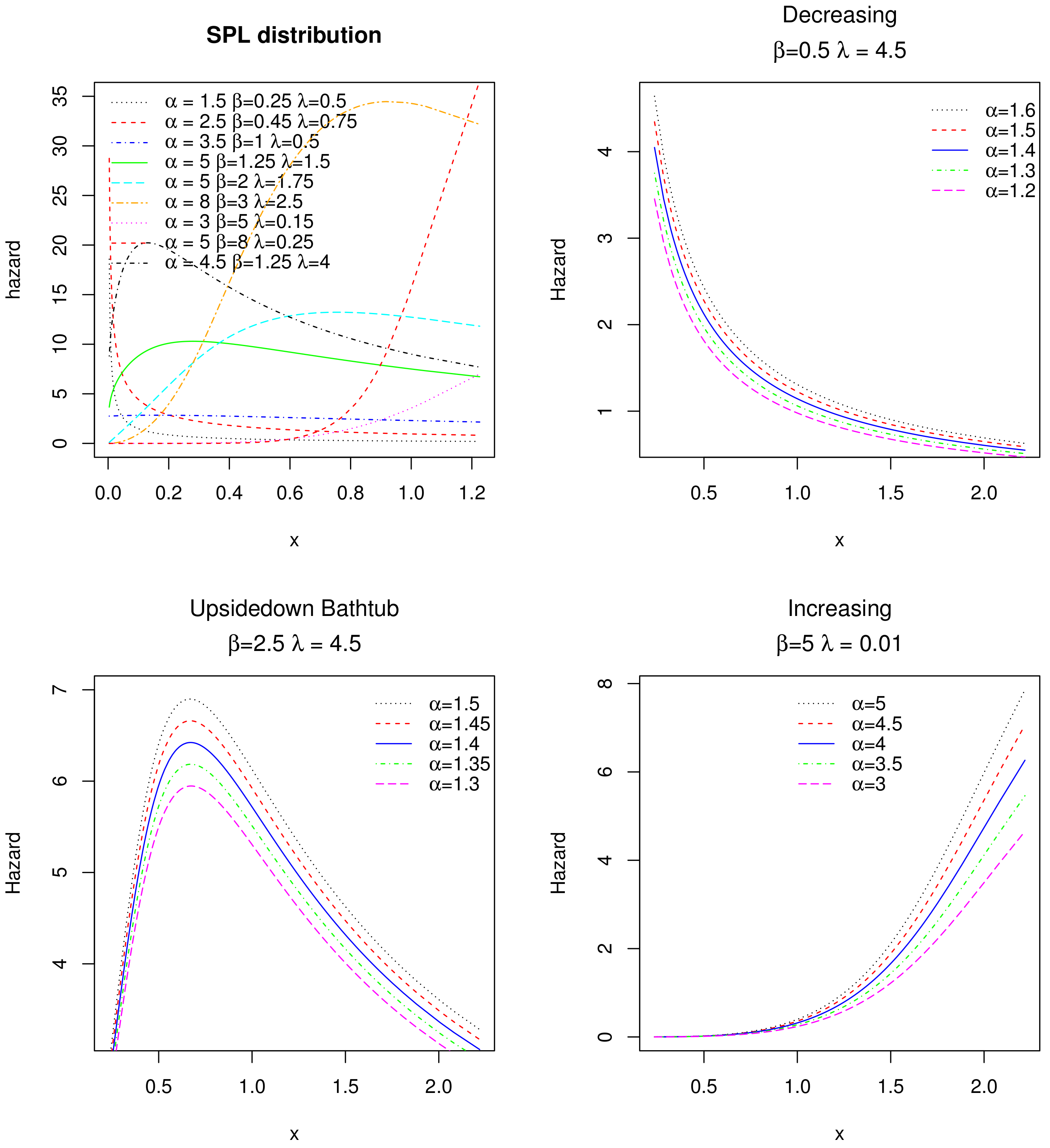
We complete this functional study by discussing the hazard rate function (hrf). First, in full generality, the hrf measures the tendency of an item to fail or die depending on the age reached. Therefore, it plays a key role in the classification of survival distributions. Basically, the shapes of hazard rates are either monotonic (increasing or decreasing) or non-monotonic (bathtub or inverted bathtub). The hrf of the SPL distribution is given by

$$h_{SPL}(x;\zeta )=\frac{\pi }{2}\alpha \beta \lambda x^{\beta -1}{(1+\lambda x^{\beta })}^{-(\alpha +1)}cot\left(\frac{\pi }{4}{(1+\lambda x^{\beta })}^{-\alpha }\right),x>0,$$

(9)

and $h_{SPL}(x;\zeta )=0$ for $x\le 0$. Upon differentiation of (9), it can be seen that $h_{SPL}(x;\zeta )$ is increasing for $\beta \ge 1$ and $\alpha \le 1$. It is also conjectured that $h_{SPL}(x;\zeta )$ is decreasing for $\beta \le 1$ and $\alpha \ge 1$, and unimodal for $\beta \ge 1$ and $\alpha \ge 1$. The graphical study in Figure 2 supports these claims.

Figure 2 emphasizes the fact that the proposed SPL distribution possesses increasing and decreasing, and also upside down bathtub hazard rates.

Another important function of the SPL distribution is the quantile function (qf). It is defined as the inverse function of the corresponding cdf. Thus, based on (7), it is specified by

$$Q(u;\zeta )=F_{SPL}^{-1}(u;\zeta )={\left\{\frac{1}{\lambda }\left[{\left(\frac{2}{\pi }arccosu\right)}^{-1/\alpha }-1\right]\right\}}^{1/\beta },u\in (0,1).$$

(10)

As the cdf, the qf determined the SPL distribution. Classically, we can use it for determining the median, as well as the lower and upper quartiles. The qf can also be used to generate values from a random variable with the SPL distribution. Further detail on the quantile-based reliability analysis can be found in [33].

2.2. Moment Analysis

We now conduct a moment analysis. The following result gives a series expansion for the (crude) moments of a random variable with the SPL distribution.

Proposition 1.

Let $r\ge 1$ be an integer and X be a random variable with the SPL distribution. Then, for $r<2\alpha \beta$, the r-th moment of X exists and can be expanded as

$$\begin{array}{c}\hfill E\left(X^r\right)=\alpha {\lambda }^{-r/\beta }\sum _{k=1}^{+\infty }\frac{{(-1)}^{k+1}}{(2k-1)!}{\left(\frac{\pi }{2}\right)}^{2k}B\left(\frac{r}{\beta }+1,2k\alpha -\frac{r}{\beta }\right),\end{array}$$

where E denotes the mathematical expectation and $B(a,b)$ refers to the standard beta function given as $B(a,b)={\int }_0^1{t}^{a-1}{(1-t)}^{b-1}dt={\int }_0^{+\infty }{t}^{a-1}{(1+t)}^{-(a+b)}dt$ for $a,b>0$.

Proof. 

First, the definition of $E\left(X^r\right)$ is

$$\begin{array}{c}\hfill E\left(X^r\right)={\int }_{-\infty }^{+\infty }{x}^r{f}_{SPL}(x;\zeta )dx={\int }_0^{+\infty }{x}^r{f}_{SPL}(x;\zeta )dx,\end{array}$$

(11)

since $f_{SPL}(x;\zeta )=0$ for $x\le 0$.

Let us study the mathematical existence of this integral by the Riemann integrability criterion. When $x\to 0$, we have $x^r{f}_{SPL}(x;\zeta )\sim (\pi /2)\alpha \beta \lambda x^{r+\beta -1}$, which is integrable over $(0,\delta )$ with $\delta >0$ since $\beta >0$. For the case $x\to +\infty$, we have $x^r{f}_{SPL}(x;\zeta )\sim ({\pi }^2/4)\alpha \beta {\lambda }^{-2\alpha }{x}^{r-2\alpha \beta -1}$, which is integrable over $(\delta ,+\infty )$ with $\delta >0$ if and only if $r<2\alpha \beta$. The desired condition is obtained.

Let us now investigate a linear representation of the cdf expressed in (7), from which we will deduce a series expansion for the pdf as given by (8). By using the Taylor series expansion of the cosine function, for $x>0$, we get

$$\begin{array}{cc}\hfill F_{SPL}(x;\zeta )& =cos\left(\frac{\pi }{2}{(1+\lambda x^{\beta })}^{-\alpha }\right)=\sum _{k=0}^{+\infty }\frac{{(-1)}^k}{\left(2k\right)!}{\left(\frac{\pi }{2}{(1+\lambda x^{\beta })}^{-\alpha }\right)}^{2k}\hfill \\ \hfill & =\sum _{k=0}^{+\infty }\frac{{(-1)}^k}{\left(2k\right)!}{\left(\frac{\pi }{2}\right)}^{2k}{(1+\lambda x^{\beta })}^{-2k\alpha }.\hfill \end{array}$$

By applying a first order differentiation with respect to x, the following series expansion of the pdf comes:

$$\begin{array}{c}\hfill f_{SPL}(x;\zeta )=\alpha \lambda \beta \sum _{k=1}^{+\infty }\frac{{(-1)}^{k+1}}{(2k-1)!}{\left(\frac{\pi }{2}\right)}^{2k}{x}^{\beta -1}{(1+\lambda x^{\beta })}^{-2k\alpha -1}.\end{array}$$

(12)

Please note that we ignored the term in $k=0$ since the corresponding term disappears. From (11) and (12), by integrating $f_{SPL}(x;\zeta )$ with respect to x, swapping the symbols ∫ and ∑ by the dominated convergence theorem, and applying the change of variables $y=\lambda x^{\beta }$, we obtain

$$\begin{array}{cc}\hfill E\left(X^r\right)& =\alpha \lambda \beta \sum _{k=1}^{+\infty }\frac{{(-1)}^{k+1}}{(2k-1)!}{\left(\frac{\pi }{2}\right)}^{2k}{\int }_0^{+\infty }{x}^{r+\beta -1}{(1+\lambda x^{\beta })}^{-2k\alpha -1}dx\hfill \\ \hfill & =\alpha {\lambda }^{-r/\beta }\sum _{k=1}^{+\infty }\frac{{(-1)}^{k+1}}{(2k-1)!}{\left(\frac{\pi }{2}\right)}^{2k}B\left(\frac{r}{\beta }+1,2k\alpha -\frac{r}{\beta }\right).\hfill \end{array}$$

This completes the proof of Proposition 1. □

A computational remark is that, for K large enough, a precise approximation of ${\mu }_r^{\prime }$ is obtained as

$$\begin{array}{cc}\hfill E\left(X^r\right)& \approx \alpha {\lambda }^{-r/\beta }\sum _{k=1}^K\frac{{(-1)}^{k+1}}{(2k-1)!}{\left(\frac{\pi }{2}\right)}^{2k}B\left(\frac{r}{\beta }+1,2k\alpha -\frac{r}{\beta }\right).\hfill \end{array}$$

Diverse moment measure can be defined from Proposition 1. Here, we restrict our attention on the variance of X basically defined by $\mathrm{Var}=E\left(X^2\right)-{\left[E\left(X\right)\right]}^2$.

The first four moments and variance of X for different parameter values are indicated in

Table 1. Moments of a random variable X with SPL distribution for different parameter values.

Parameters	$\mathit{\alpha }$	$\mathit{E}\left(\mathit{X}\right)$	$\mathit{E}\left({\mathit{X}}^2\right)$	$\mathit{E}\left({\mathit{X}}^3\right)$	$\mathit{E}\left({\mathit{X}}^4\right)$	Var
$\beta =1.15$  $\lambda =0.05$	5	2.0982958	8.0587805	46.731802	380.750565	3.6559354
	10	1.0965961	2.1021457	5.766650	20.843274	0.8996228
	15	0.7593655	0.9941883	1.835014	4.389999	0.4175523
	20	0.5869620	0.5900577	0.830389	1.503360	0.2455333
$\beta =0.95$  $\lambda =0.15$	2.5	1.9969643	10.875856	141.228274	5891.000628	6.8879901
	3.5	1.2950962	4.065762	24.541340	276.793358	2.3884878
	4	1.0991066	2.838471	13.451765	110.208386	1.6304353
	6	0.6802299	1.019179	2.569788	9.906019	0.5564665

provided $\alpha \beta >2$.

From Table 1, we see the numerical versatility of the moment measures considered, varying from small to large values; central and dispersion indicators may be negligible or substantial. This confirms the claim about the overall flexibility of the SPL distribution.

Based on similar developments employed in the proof Proposition 1, it is possible to express various series expansions of moment-type functions. Here, we complete our moment analysis by investigating the incomplete moments of the SPL distribution which are involved in the definition of many applied measures and indicators.

Proposition 2.

Let $r\ge 1$ be an integer, $t\ge 0$ and X be a random variable with the SPL distribution. Then, the r-th incomplete moment of X with the truncated value t exists and can be expanded as

$$\begin{array}{c}\hfill E\left(X^{r}I(X\le t)\right)=\alpha {\lambda }^{-r/\beta }\sum _{k=1}^{+\infty }\frac{{(-1)}^{k+1}}{(2k-1)!}{\left(\frac{\pi }{2}\right)}^{2k}{B}_{\lambda t^{\beta }/(1+\lambda t^{\beta })}\left(\frac{r}{\beta }+1,2k\alpha -\frac{r}{\beta }\right),\end{array}$$

where I denotes the indicator function and $B_u(a,b)$ refers to the truncated beta function given as $B_u(a,b)={\int }_0^u{t}^{a-1}{(1-t)}^{b-1}dt$ for $a,b>0$ and $u\in (0,1)$.

Proof. 

First, we have

$$\begin{array}{c}\hfill E\left(X^{r}I(X\le t)\right)={\int }_0^t{x}^r{f}_{SPL}(x;\zeta )dx.\end{array}$$

(13)

The rest of the development follows the lines of the proof of Proposition 1; From (12) and (13), by integrating $f_{SPL}(x;\zeta )$ with respect to x, swapping the symbols ∫ and ∑ owing to the dominated convergence theorem, and applying the change of variables $y=\lambda x^{\beta }$, we obtain

$$\begin{array}{cc}\hfill E\left(X^{r}I(X\le t)\right)& =\alpha \lambda \beta \sum _{k=1}^{+\infty }\frac{{(-1)}^{k+1}}{(2k-1)!}{\left(\frac{\pi }{2}\right)}^{2k}{\int }_0^t{x}^{r+\beta -1}{(1+\lambda x^{\beta })}^{-2k\alpha -1}dx\hfill \\ \hfill & =\alpha {\lambda }^{-r/\beta }\sum _{k=1}^{+\infty }\frac{{(-1)}^{k+1}}{(2k-1)!}{\left(\frac{\pi }{2}\right)}^{2k}{\int }_0^{\lambda t^{\beta }}{y}^{r/\beta }{(1+y)}^{-2k\alpha -1}dy.\hfill \end{array}$$

Next, with the change of variables $z=y/(1+y)$, we get

$$\begin{array}{cc}\hfill E\left(X^{r}I(X\le t)\right)& =\alpha {\lambda }^{-r/\beta }\sum _{k=1}^{+\infty }\frac{{(-1)}^{k+1}}{(2k-1)!}{\left(\frac{\pi }{2}\right)}^{2k}{\int }_0^{\lambda t^{\beta }/(1+\lambda t^{\beta })}{z}^{r/\beta }{(1-z)}^{2k\alpha -r/\beta -1}dz\hfill \\ \hfill & =\alpha {\lambda }^{-r/\beta }\sum _{k=1}^{+\infty }\frac{{(-1)}^{k+1}}{(2k-1)!}{\left(\frac{\pi }{2}\right)}^{2k}{B}_{\lambda t^{\beta }/(1+\lambda t^{\beta })}\left(\frac{r}{\beta }+1,2k\alpha -\frac{r}{\beta }\right).\hfill \end{array}$$

This completes the proof of Proposition 2. □

Based on the incomplete moments, we can define the mean residual life function, mean waiting time, mean deviation about the mean, and various inequalities measures (Lorenz curve, Gini index, Bonferroni curve, Atkinson index, Zenga index, Pietra index, etc.). In this regard, we may refer the reader to the book of [34]. However, these measures are beyond the applied line of this paper.

3. Inference of the SPL Model

This section is devoted to the inferential treatment of the SPL distribution for the perspectives of statistical modelling. The maximum likelihood method, as described in full generality in [35], is employed. A mathematical description of this method in the context of the SPL distribution is provided below.

First, let $x_1,x_2,\dots x_n$ be observations drawn from a random variable X with the SPL distribution. Then the corresponding likelihood function and log-likelihood function are

$$L_{SPL}\left(\zeta \right)={\left(\frac{\pi }{2}\right)}^n{\left(\alpha \beta \lambda \right)}^n\prod _{i=1}^n{x}_i^{\beta -1}{(1+\lambda x_i^{\beta })}^{-(\alpha +1)}sin\left(\frac{\pi }{2}{(1+\lambda x_i^{\beta })}^{-\alpha }\right)$$

and

$$\begin{array}{cc}\hfill log{L}_{SPL}\left(\zeta \right)& =nlog\left(\frac{\pi }{2}\right)+nlog\left(\alpha \beta \lambda \right)+(\beta -1)\sum _{i=1}^{n}log{x}_i-(\alpha +1)\sum _{i=1}^{n}log(1+\lambda x_i^{\beta })\hfill \\ \hfill & +\sum _{i=1}^{n}log\left(sin\left(\frac{\pi }{2}{(1+\lambda x_i^{\beta })}^{-\alpha }\right)\right),\hfill \end{array}$$

respectively. Then, the maximum likelihood estimates (MLEs) are defined by $\widehat{\zeta }$=$argma{x}_{\zeta }{L}_{SPL}\left(\zeta \right)$ = $argma{x}_{\zeta }[log{L}_{SPL}\left(\zeta \right)]$. The components of $\widehat{\zeta }$, say $\widehat{\alpha }$, $\widehat{\beta }$ and $\widehat{\lambda }$, form the MLEs of $\alpha$, $\beta$ and $\lambda$, respectively. The MLEs can be formalized through non-linear equations involving the partial differentiation of the log-likelihood function with respect to the parameters $\alpha$, $\beta$ and $\lambda$. These partial derivatives are given as

$$\begin{array}{cc}\hfill \frac{\partial }{\partial \alpha }log{L}_{SPL}\left(\zeta \right)& =\frac{n}{\alpha }-\sum _{i=1}^{n}log(1+\lambda x_i^{\beta })-\frac{\pi }{2}\sum _{i=1}^n{(1+\lambda x_i^{\beta })}^{-\alpha }log(1+\lambda x_i^{\beta })\times \hfill \\ \hfill & cot\left(\frac{\pi }{2}{(1+\lambda x_i^{\beta })}^{-\alpha }\right)\hfill \end{array}$$

$$\begin{array}{cc}\hfill \frac{\partial }{\partial \beta }log{L}_{SPL}\left(\zeta \right)& =\frac{n}{\beta }+\sum _{i=1}^{n}log{x}_i-(\alpha +1)\lambda \sum _{i=1}^n\frac{x_i^{\beta }}{1+\lambda x_i^{\beta }}log{x}_i-\frac{\pi }{2}\alpha \lambda \sum _{i=1}^n{x}_i^{\beta }log{x}_i\times \hfill \\ \hfill & {(1+\lambda x_i^{\beta })}^{-\alpha -1}cot\left(\frac{\pi }{2}{(1+\lambda x_i^{\beta })}^{-\alpha }\right)\hfill \end{array}$$

and

$$\begin{array}{c}\hfill \frac{\partial }{\partial \lambda }log{L}_{SPL}\left(\zeta \right)=\frac{n}{\lambda }-(\alpha +1)\sum _{i=1}^n\frac{x_i^{\beta }}{1+\lambda x_i^{\beta }}-\frac{\pi }{2}\alpha \sum _{i=1}^n{x}_i^{\beta }{(1+\lambda x_i^{\beta })}^{-\alpha -1}cot\left(\frac{\pi }{2}{(1+\lambda x_i^{\beta })}^{-\alpha }\right).\end{array}$$

Simple analytical expressions for $\widehat{\alpha }$, $\widehat{\beta }$ and $\widehat{\lambda }$ remain impossible, but practice only requires numerical evaluations of them. These numerical values can be easily obtained using specific tools in statistical software as the R software (see [36]). Also, the well-established theory on MLEs ensures that the random version of $\widehat{\zeta }$ is asymptotically three-dimensional normal with mean vector $\zeta$ and variance-covariance matrix $V={\{-{\nabla }_{\zeta }^{2}log{L}_{SPL}\left(\zeta \right){\mid }_{\zeta =\widehat{\zeta }}\}}^{-1}$, where ${\nabla }_{\xi }$ denotes the gradient according to $\xi$.

In particular, the (asymptotic) estimated standard error (SE) of $\widehat{\alpha }$ is obtained by taking the square-root of the first diagonal component of V, and we can proceed in a similar way to obtain the SEs of the two other parameters. The asymptotic normal distribution is at the basis of diverse statistical tests or confidence intervals. Also, based on $\widehat{\xi }$, $f_{SPL}(x;\widehat{\zeta })$ is the estimated pdf of $f_{SPL}(x;\zeta )$. This estimated pdf plays a central role in fitting the normalized histogram of the data, as discussed in the next section on applications.

We now evaluate the accuracy of the MLEs of the SPL model. The data are artificial; they are generated by using the qf as defined by (10) through the inverse transform sampling technique. We conduct 1000 Monte Carlo simulations for each sample size n with $n=50$, 100, 200, 300 and 500 to the following different sets of parameters: Set I $=(0.5,1.5,0.5)$, Set II $=(1.25,1.25,0.5)$, Set III $=(1.5,1.5,0.5)$ and Set IV $=(1.5,2.5,0.5)$ with reference to the usual order $(\alpha ,\beta ,\lambda )$. In each case, the standard mean MLE (MMLE), bias (Bias) and mean squared error (MSE) are calculated. The results are reported in

Table 2. Results of the simulation study for the SPL model.

n	$\widehat{\mathit{\alpha }}$			$\widehat{\mathit{\beta }}$			$\widehat{\mathit{\lambda }}$
	MMLE	Bias	MSE	MMLE	Bias	MSE	MMLE	Bias	MSE
					Set I
50	1.108839	0.6088391	11.32678	1.614203	0.1142034	0.243457	0.7196926	0.2196926	6.40414
100	0.6011519	0.1011519	0.1436395	1.540166	0.04016637	0.08303307	0.547555	0.04755502	0.1272187
200	0.5293078	0.02930776	0.03047932	1.526763	0.0267628	0.03582971	0.5289976	0.02899762	0.04151895
300	0.5133177	0.01331768	0.01382865	1.522277	0.02227688	0.0221875	0.5196845	0.01968455	0.02336737
500	0.5128972	0.01289724	0.008065997	1.50705	0.007049975	0.01270958	0.5059856	0.0059856	0.01260153
					Set II
50	6.468901	5.218901	159.0966	1.329557	0.07955683	0.1083518	1.110171	0.6101705	37.25226
100	3.593558	2.343558	54.05308	1.265795	0.01579527	0.03209507	0.5524636	0.05246365	0.2133836
200	1.859037	0.6090371	5.817042	1.257794	0.007794238	0.01795586	0.5249296	0.0249296	0.1045979
300	1.514497	0.2644969	1.594299	1.257145	0.007145333	0.01171177	0.5257128	0.02571277	0.06209381
500	1.38347	0.13347	0.4142243	1.251482	0.001482267	0.006478437	0.5039528	0.0039528	0.02902843
					Set III
50	9.361844	7.861844	305.6011	1.59088	0.09087955	0.1409131	0.9202953	0.4202953	7.984993
100	4.759137	3.259137	72.48332	1.519314	0.01931441	0.05390178	0.5778875	0.07788749	0.42830
200	2.467968	0.9679683	14.13403	1.521203	0.02120301	0.02278287	0.5443301	0.04433006	0.1120899
300	2.006722	0.5067219	4.919388	1.506562	0.006562497	0.01653096	0.5164482	0.01644821	0.07516359
500	1.66471	0.1647104	0.4900911	1.507026	0.007025808	0.009009118	0.5154791	0.01547907	0.03658865
					Set IV
50	8.911521	7.411521	314.756	2.675421	0.1754205	0.3928405	1.104784	0.6047839	37.61909
100	4.948069	3.448069	100.0595	2.546041	0.04604129	0.14232	0.5919749	0.09197495	0.3972336
200	2.477961	0.977961	14.33094	2.529503	0.02950304	0.07370563	0.5540613	0.05406125	0.1307966
300	1.877404	0.3774044	2.798978	2.518045	0.01804488	0.04578572	0.5330729	0.03307289	0.07655854
500	1.764778	0.2647782	1.438529	2.501113	0.00111261	0.02642756	0.4970354	-0.002964561	0.03740574

.

From Table 2, we see that the maximum likelihood method performs quite well to estimate the parameters for the considered sample sizes. Indeed, as the sample size increases, the biases and the SEs of the MLEs decrease as expected. Also, we observe that when the sample size increases, the MMLEs are closed to the true parameter values.

We now present some useful measures of adequacy by using the notation of the SPL distribution for convenience. Let $x_1,x_2,\dots ,x_n$ be the data and $x_{\left(1\right)},x_{\left(2\right)},\dots ,x_{\left(n\right)}$ be their ordered values. First, we consider the Cramér-von Mises (W*), Anderson Darling (A*) and Kolmogorov-Smirnov (K-S) statistics ($D_n$) defined by

$$\mathrm{W}*=\frac{1}{12n}+\sum _{i=1}^n{\left[F_{SPL}(x_{\left(i\right)};\widehat{\zeta })-\frac{2i-1}{n}\right]}^2,$$

$$\mathrm{A}*=-n-\sum _{i=1}^n\frac{2i-1}{n}\left[log(F_{SPL}(x_{\left(i\right)};\widehat{\zeta }))+log(1-F_{SPL}(x_i;\widehat{\zeta }))\right]$$

and

$$D_n=\underset{i=1,\dots ,n}{max}\left(\frac{i}{n}-F_{SPL}(x_{\left(i\right)};\widehat{\zeta }),F_{SPL}(x_{\left(i\right)};\widehat{\zeta })-\frac{i-1}{n}\right),$$

respectively, where $\zeta$ denotes the parameters of the distribution, i.e., $\zeta =(\alpha ,\beta ,\lambda )$ for the SPL distribution and $\widehat{\zeta }$ for its MLE. The p-Value of the K-S test related to $D_n$ is also considered. The above definitions can be adapted for any other distribution by changing the definition of the cdf and the notation of the parameters. These adequacy measures are widely used to find out which model is best suited. The model with the minimum value for W* or A*, and maximum value for p-Value, is chosen as the best one that is in adequacy to the data.

Also, we consider the Akaike information criterion (AIC), corrected Akaike information criterion (CAIC), Bayesian information criterion (BIC) and Hannan-Quinn information criterion (HQIC), defined in the context of the SPL distribution as

$$\begin{array}{cccc}\hfill \mathrm{AIC}& =-2log{L}_{SPL}(x;\widehat{\zeta })+2k,\hfill & \hfill \mathrm{BIC}& =-2log{L}_{SPL}(x;\widehat{\zeta })+klog\left(n\right),\hfill \\ \hfill \mathrm{CAIC}& =-2log{L}_{SPL}(x;\widehat{\zeta })+\frac{2kn}{n-k-1},\hfill & \hfill \mathrm{HQIC}& =-2log{L}_{SPL}(x;\widehat{\zeta })+2klog[log\left(n\right)],\hfill \end{array}$$

respectively, where k is the number of parameters so $k=3$ for the SPL distribution. As commonly accepted, the model with the minimum value for AIC or CAIC or BIC or HQIC is chosen as the best one that fits the data. Further informations on the use and interpretation of the measures W*, A*, AIC, CAIC, BIC and HQIC can be found in [37].

In this study, we aim to compare the SPL model related to the SPL distribution with the useful and competitive Lomax-type model listed in

Table 3. Competitive models of the SPL model.

Models	Abbreviations	Cdfs ($\mathit{x}>0$)	References
Topp-Leone Lomax	TLGL	${\displaystyle {\left(1-{(1+\alpha x)}^{-2\beta }\right)}^{\lambda }}$	[38]
power Lomax	PL	${\displaystyle 1-{\left(1+\lambda x^{\beta }\right)}^{-\alpha }}$	[17]
exponentiated Lomax	EL	${\displaystyle {\left(1-{\left(\frac{\beta }{x+\beta }\right)}^{\alpha }\right)}^{\lambda }}$	[39]
Lomax	Lomax	${\displaystyle 1-{\left(\frac{\beta }{x+\beta }\right)}^{\lambda }}$	[18]

.

We can notice that the Lomax model is nested in the TLGL, EL and PL models. The proposed SPL model is completely different in this sense. In addition, conceptually, the TLGL and EL models are closed; they coincide with a reparametrization of the parameters.

4. Applications of the SPL Model

Based on the above methodology, we apply the SPL model on nine datasets. They differ mainly in size, characteristics or background, but all of them are of modern interest to their respective fields. For each dataset, we proceed as follows:

• We briefly present the data, with reference(s).
• We provide a table that summarizes the main statistical characteristics of the data.
• We assess the quality of the fit measures of the models considered and organize them in a table in order of the model performance.
• As complementary work, we indicate the MLES of the model parameters as well as the related SEs.
• We end with a visual approach by plotting the histogram of the data and the fitted pdfs, and, in another graph, the probability-probability (PP) plot for the SPL model only.

Data set 1: We consider a real dataset on the remission times (in months) of a random sample of 128 bladder cancer patients. This dataset is given by Lee and Wang [40] and it contains the following values: 0.08, 2.09, 3.48, 4.87, 6.94, 8.66, 13.11, 23.63, 0.20, 2.23, 3.52, 4.98, 6.97, 9.02, 13.29, 0.40, 2.26, 3.57, 5.06, 7.09, 9.22, 13.80, 25.74, 0.50, 2.46, 3.64, 5.09, 7.26, 9.47, 14.24, 25.82, 0.51, 2.54, 3.70, 5.17, 7.28, 9.74, 14.76, 26.31, 0.81, 2.62, 3.82, 5.32, 7.32, 10.06, 14.77, 32.15, 2.64, 3.88, 5.32, 7.39, 10.34, 14.83, 34.26, 0.90, 2.69, 4.18, 5.34, 7.59, 10.66, 15.96, 36.66, 1.05, 2.69, 4.23, 5.41, 7.62, 10.75, 16.62, 43.01, 1.19, 2.75, 4.26, 5.41, 7.63, 17.12, 46.12, 1.26, 2.83, 4.33, 5.49, 7.66, 11.25, 17.14, 79.05, 1.35, 2.87, 5.62, 7.87, 11.64, 17.36, 1.40, 3.02, 4.34, 5.71, 7.93, 11.79, 18.10, 1.46, 4.40, 5.85, 8.26, 11.98, 19.13, 1.76, 3.25, 4.50, 6.25, 8.37, 12.02, 2.02, 3.31, 4.51, 6.54, 8.53, 12.03, 20.28, 2.02, 3.36, 6.76, 12.07, 21.73, 2.07, 3.36, 6.93, 8.65, 12.63, 22.69.

A summary measure of descriptive statistics of dataset 1 is provided in

Table 4. Descriptive statistics of dataset 1.

Mean	Median	Variance	Skewness	Kurtosis	Minimum	Maximum
9.36562	6.395	110.425	3.28657	15.48308	0.08	79.05

.

We see in Table 4 that the data are right skewed and highly leptokurtic with high variance. With respect to model adequacy, the measures W*, A*, $D_n$, p-Value, AIC, CAIC, BIC and HQIC are reported in

Table 5. Goodness of fit measures of the models for dataset 1

Models	W*	A*	${\mathit{D}}_{\mathit{n}}$	p-Value	AIC	CAIC	BIC	HQIC
SPL	0.0186	0.1239	0.0349	0.9977	825.3925	825.5861	833.9486	828.8689
PL	0.0195	0.1308	0.0351	0.9974	825.4798	825.6733	834.0359	828.9562
TLGL	0.0283	0.1902	0.0405	0.9847	826.1436	826.3372	834.6997	829.6200
EL	0.0283	0.1902	0.0404	0.9847	826.1436	826.3372	834.6997	829.6200
Lomax	0.0807	0.4876	0.0966	0.1831	831.6658	831.7618	837.3698	833.9834

.

From Table 5, we observe that the SPL model possesses the lowest values for W*, A*, $D_n$, AIC, CAIC, BIC and HQIC, and the highest value for p-Value compared to the other models. It can be considered the best. The second best model is the PL model.

Please note that for this dataset, the results for the TLGL and EL models are almost identical due to their similar nature, but small numerical variations are observed without rounding.

For additional information, the MLEs of the model parameters as well as their SEs are reported in

Table 6. MLEs of the model parameters for dataset 1 (in parenthesis are the SEs).

Models	$\mathit{\alpha }$	$\mathit{\beta }$	$\mathit{\lambda }$
SPL	1.0216200 (0.45875225)	1.3956063 (0.18303304)	0.0371991 (0.01408465)
PL	2.070725 (0.9705209)	1.427499 (0.1782097)	34.861099 (13.9162924)
TLGL	1.586149 (0.2798032)	2.292993 (1.1137263)	24.744613 (16.6935617)
EL	4.589053 (2.2316031)	24.763807 (16.7230668)	1.586145 (0.2798554)
Lomax	-	13.96063 (15.45659)	121.24393 (143.40888)

.

From Table 6, among other, we see that the parameters $\alpha$, $\beta$ and $\lambda$ of the SPL model have been estimated by $\widehat{\alpha }=1.0216200$, $\widehat{\beta }=1.3956063$ and $\widehat{\lambda }=0.0371991$, respectively, with quite small SEs.

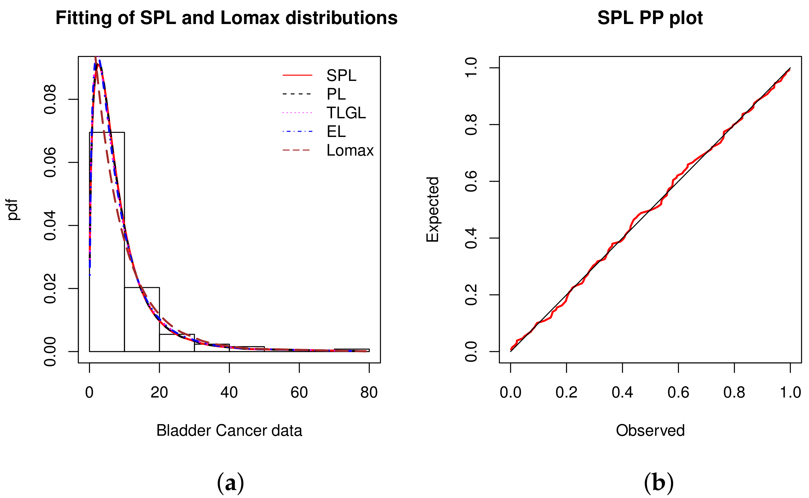
Figure 3 shows two graphics: the histogram of the data fitted by the estimated pdfs, and the PP plot for the SPL model only.

In Figure 3, we observe that the empirical objects are almost perfectly adjusted by the estimated objects. In particular, in the PP plot, the black line is almost confused with the estimated red line related to the SPL model.

Data set 2: The considered data represent the failure times of the mechanical components of the aircraft windshield. They are taken from [41]. They were recently reviewed by [42]. The data are: 0.040, 1.866, 2.385, 3.443, 0.301, 1.876, 2.481, 3.467, 0.309, 1.899, 2.610, 3.478, 0.557, 1.911, 2.625, 3.578, 0.943, 1.912, 2.632, 3.595, 1.070, 1.914, 2.646, 3.699, 1.124, 1.981, 2.661, 3.779, 1.248, 2.010, 2.688, 3.924, 1.281, 2.038, 2.823, 4.035, 1.281, 2.085, 2.890, 4.121, 1.303, 2.089, 2.902, 4.167, 1.432, 2.097, 2.934, 4.240, 1.480, 2.135, 2.962, 4.255, 1.505, 2.154, 2.964, 4.278, 1.506, 2.190, 3.000, 4.305, 1.568, 2.194, 3.103, 4.376, 1.615, 2.223, 3.114, 4.449, 1.619, 2.224, 3.117, 4.485, 1.652, 2.229, 3.166, 4.570, 1.652, 2.300, 3.344, 4.602, 1.757, 2.324, 3.376, 4.663.

A summary of descriptive statistics for dataset 2 is provided in

Table 7. Descriptive statistics of dataset 2

Mean	Median	Variance	Skewness	Kurtosis	Minimum	Maximum
2.55745	2.3545	1.25177	0.09949	−0.65232	0.04	4.663

.

Based on the information of Table 7, we can say that the data are approximately symmetric and platykurtic, with little dispersion. One more point, we observe that the data have a negative kurtosis value which means that the underlying distributions should have lighter tails.

The statistical measures considered for the comparison of the models are given in

Table 8. Goodness of fit measures of the models for dataset 2.

Models	W*	A*	${\mathit{D}}_{\mathit{n}}$	p-Value	AIC	CAIC	BIC	HQIC
SPL	0.0626	0.6447	0.0563	0.9531	268.5388	268.8388	275.8312	271.4703
PL	0.1031	0.9686	0.1061	0.3016	275.1259	275.4259	282.4184	278.0574
EL	0.2393	1.8777	0.1236	0.1536	288.6155	288.9155	295.9079	291.5470
TLGL	0.2465	1.9232	0.1204	0.1751	289.4639	289.7639	296.7563	292.3954
Lomax	0.1933	1.5824	0.3077	2.49$\times {10}^{-7}$	337.4818	337.6299	342.3434	339.4361

.

From Table 8, the values of the model adequacy measures and goodness of fit test are clearly in favor of the SPL model. The second best model is the PL model.

The MLEs of the parameters of the SPL model and other models with their SEs are reported in

Table 9. MLEs of the model parameters for dataset 2 (in parenthesis are the SEs).

Models	$\mathit{\alpha }$	$\mathit{\beta }$	$\mathit{\lambda }$
SPL	2.97275466 (1.266693742)	2.44917417 (0.234312750)	0.01610661 (0.007105774)
PL	2.510918 (1.0039915)	2.501948 (0.2813778)	24.858636 (8.8454850)
EL	24.107930 (13.9109419)	30.212370 (18.6585652)	3.661293 (0.6506768)
TLGL	3.721336 (0.7759183)	9.745047 (5.5473841)	24.585348 (16.2933590)
Lomax	-	8.650051 (3.207235)	21.150309 (8.180986)

.

In addition, the estimated pdfs over the histogram and PP plot of the SPL model are displayed in Figure 4.

From Figure 4, it is obvious that the light tails of the SPL model are instrumental in having a better fit. In addition, the PP plot underlines this power of adaptation; the black line is almost confused with the estimated red line.

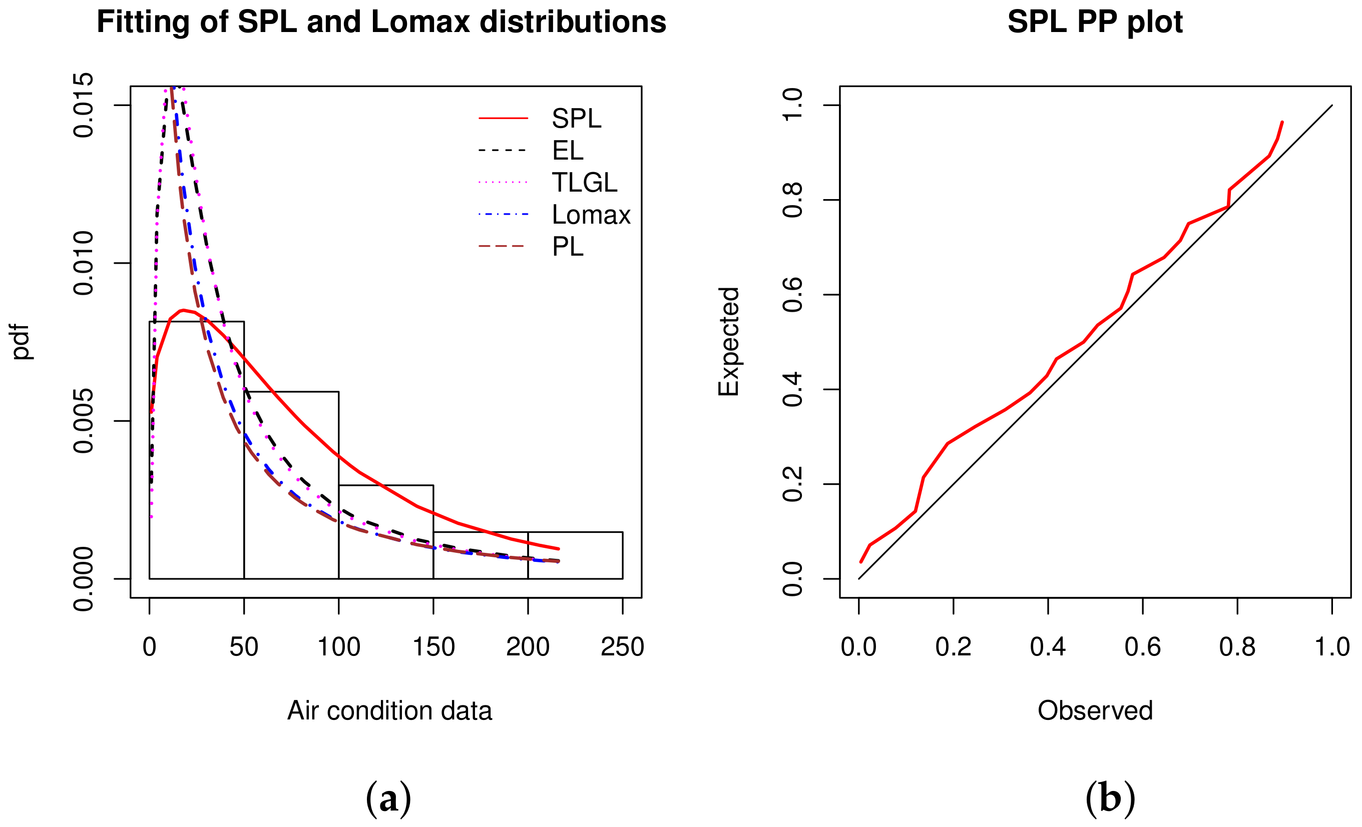
Data set 3: We now consider a dataset containing 27 observations of time of successive failures of the air conditioning system of jets in a fleet of Boeing 720 as reported in Proschan [43]. Recently, this data was studied by [44] and the data are: 1, 4, 11, 16, 18, 18, 18, 24, 31, 39, 46, 51, 54, 63, 68, 77, 80, 82, 97, 106, 111, 141, 142, 163, 191, 206, 216.

Some descriptive measures of dataset 3 are provided in

Table 10. Descriptive statistics of dataset 3.

Mean	Median	Variance	Skewness	Kurtosis	Minimum	Maximum
76.81481	63	4059.311	0.80235	−0.42669	1	216

.

From Table 10, we see that the data are right skewed and platykurtic with a high variance.

Table 11. Goodness of fit measures of the models for dataset 3.

Models	W*	A*	${\mathit{D}}_{\mathit{n}}$	p-Value	AIC	CAIC	BIC	HQIC
SPL	0.0379	0.2811	0.1023	0.9399	296.0297	297.0732	299.9172	297.1857
EL	0.1396	0.9252	0.1609	0.4865	304.4668	305.5103	308.3543	305.6228
TLGL	0.1623	1.0683	0.1738	0.3880	306.2415	307.285	310.129	307.3975
PL	0.0932	0.6368	0.2345	0.1025	309.2454	310.2889	313.133	310.4014
Lomax	0.1052	0.7090	0.2161	0.1605	306.0443	306.5443	308.6359	306.8149

indicates the values of the statistical measures considered to compare the models.

The analysis of Table 11 ensures that the SPL model is the best with, in particular, p-Value $=0.9399$. The second best model is the EL model.

The MLEs of the model parameters as well as their SEs are reported in

Table 12. MLEs of the model parameters for dataset 3 (in parenthesis are the SEs).

Models	$\mathit{\alpha }$	$\mathit{\beta }$	$\mathit{\lambda }$
SPL	1.382763741 (0.6448660998)	1.221321892 (0.1405012622)	0.002328135 (0.0004797677)
EL	1.123151 (0.3229477)	17.681731 (10.9965985)	2.336629 (0.7915584)
TLGL	2.8564521 (1.0394244)	0.5234784 (0.1417636)	11.9763851 (7.9755583)
PL	1.1193937 (0.5529827)	0.8687552 (0.1596078)	24.1383129 (10.1687168)
Lomax	-	0.9108902 (0.2758631)	29.3494386 (12.4143031)

.

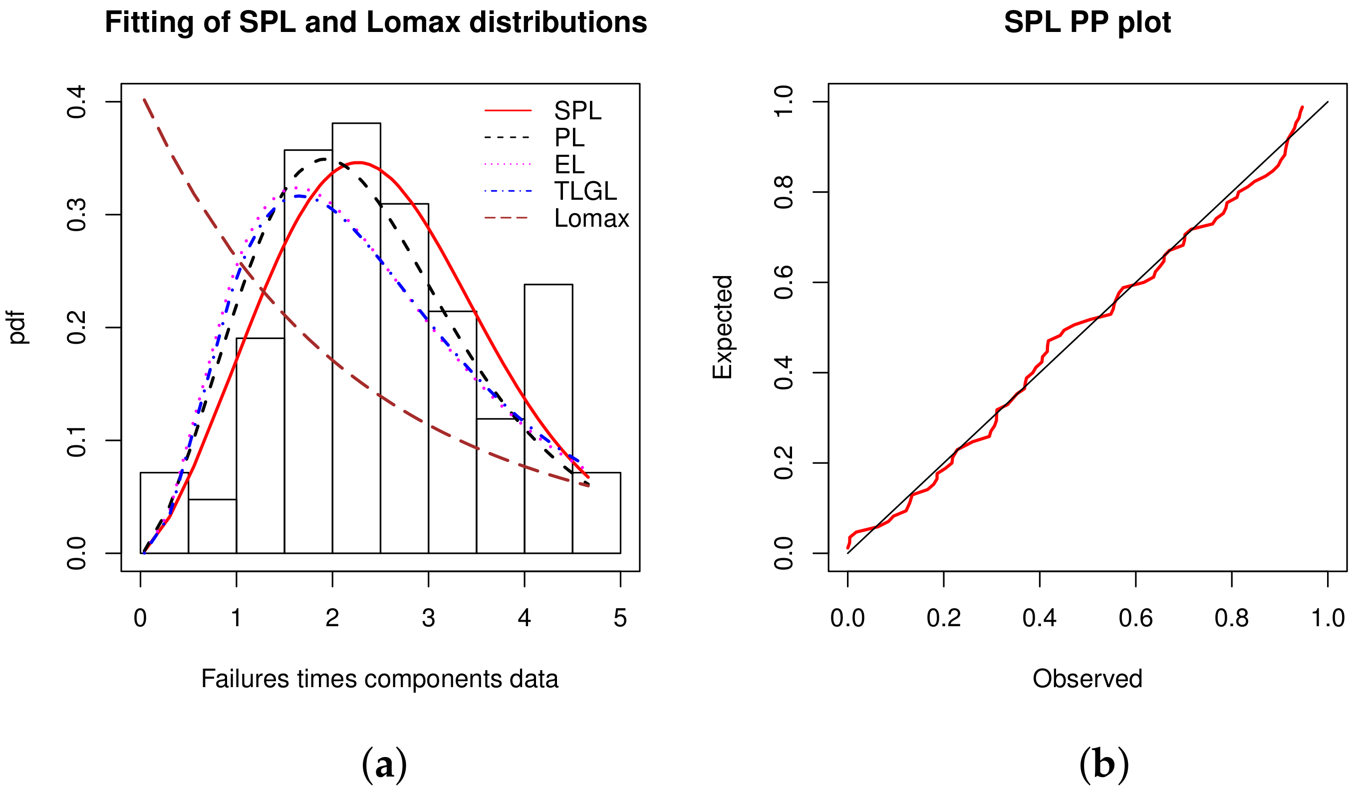
The estimated pdfs over the histogram and the PP plot of the SPL model are shown in Figure 5.

In Figure 5, the fitted power of the SPL model is flagrant; the corresponding estimated pdf has captured the decreasing roundness shape of the histogram, contrary to the other estimated pdfs. In addition, the red line of the PP plot is generally close to the black line.

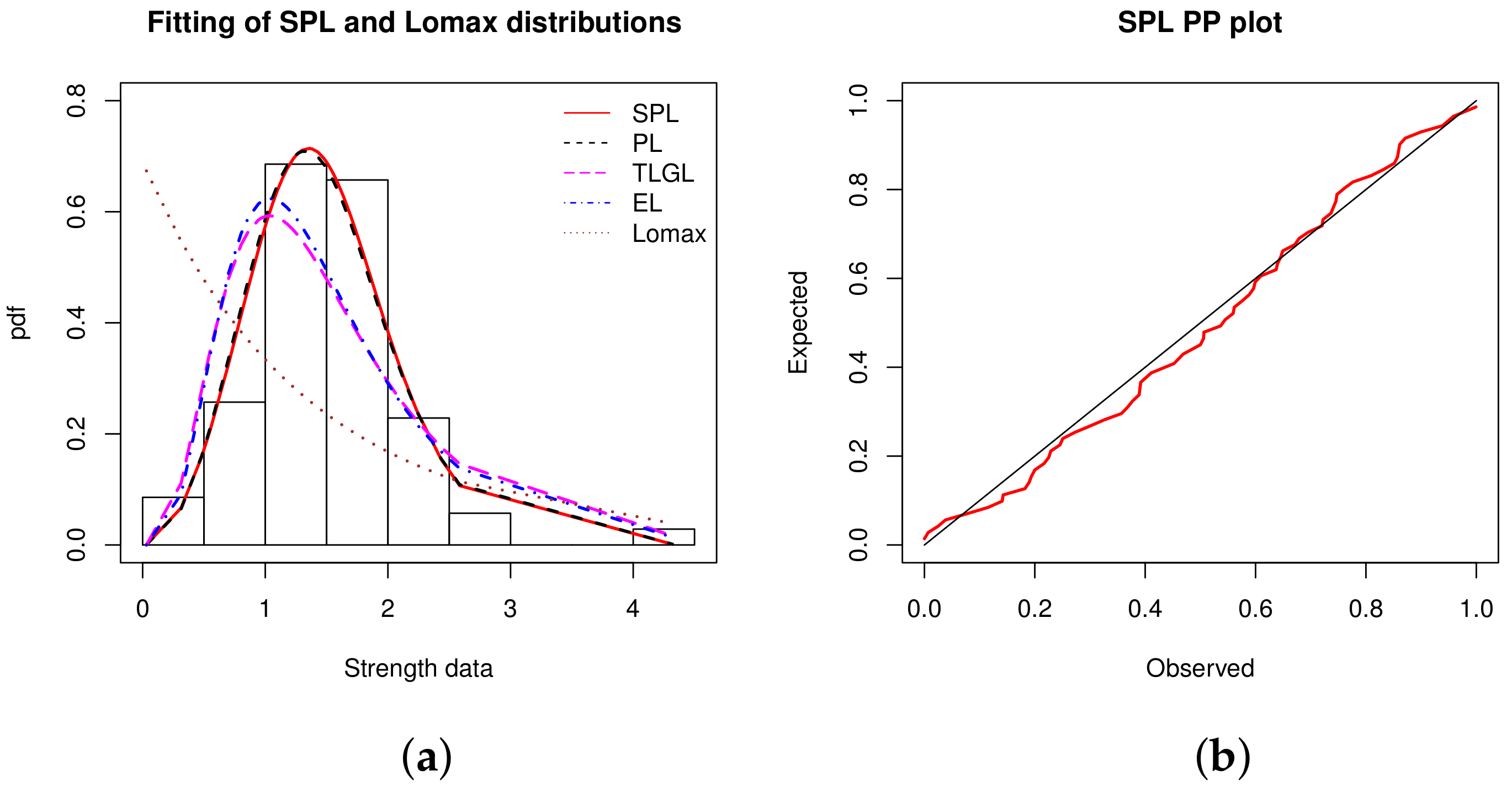
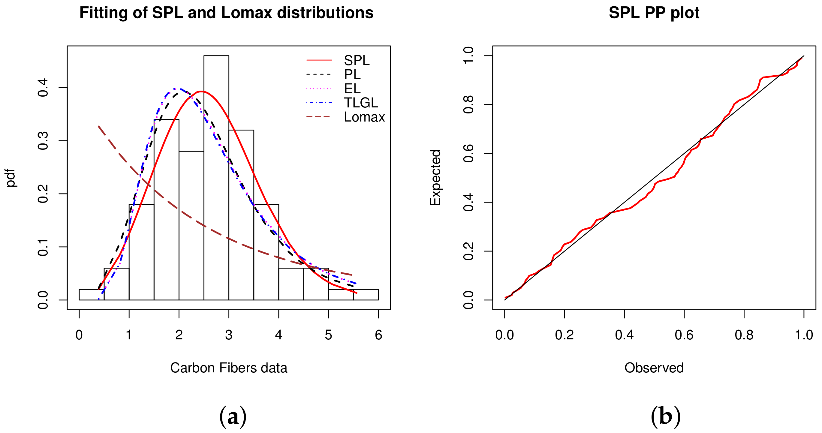
Data set 4: The data represent 69 strength measures for single carbon fibers (and impregnated 1000-carbon fiber tows). They are given by [45]. The measures in GPA by subtracting 1 are: 0.0312, 0.314, 0.479, 0.552, 0.700, 0.803, 0.861, 0.865, 0.944, 0.958, 0.966, 0.977, 1.006, 1.021, 1.027, 1.055, 1.063, 1.098, 1.140, 1.179, 1.224, 1.240, 1.253, 1.270, 1.272, 1.274, 1.301, 1.301, 1.359, 1.382, 1.382, 1.426, 1.434, 1.435, 1.478, 1.490, 1.511, 1.514, 1.535, 1.554, 1.566, 1.570, 1.586, 1.629, 1.633, 1.642, 1.648, 1.684, 1.697, 1.726, 1.770, 1.773, 1.800, 1.809, 1.818, 1.821, 1.848, 1.880, 1.954, 2.012, 2.067, 2.084, 2.090, 2.096, 2.128, 2.233, 2.433, 2.585, 2.585,4.32.

A statistical description of dataset 4 is given in

Table 13. Descriptive statistics of dataset 4.

Mean	Median	Variance	Skewness	Kurtosis	Minimum	Maximum
1.48802	1.484	0.3702	1.24191	5.46869	0.0312	4.32

.

Table 13 shows that the data are almost symmetric and leptokurtic, with a low variance.

The fitting performance of the considered models are investigated numerically in

Table 14. Goodness of fit measures of the models for dataset 4.

Models	W*	A*	${\mathit{D}}_{\mathit{n}}$	p-Value	AIC	CAIC	BIC	HQIC
SPL	0.1218	0.8688	0.0720	0.8614	131.0550	131.4187	137.8005	133.7344
PL	0.1345	0.9450	0.0778	0.7909	131.9917	132.3553	138.7372	134.6711
TLGL	0.4060	2.5291	0.1443	0.1085	152.7280	153.0916	159.4734	155.4073
EL	0.4265	2.6440	0.1440	0.1098	153.4122	153.7758	160.1577	156.0916
Lomax	0.3213	2.0540	0.3554	4.18$\times {10}^{-8}$	204.3163	204.4954	208.8133	206.1026

.

From Table 14, we see that the SPL model is more relevant for the fit of the dataset than the other models. Indeed, it has the lowest value for all the statistical measures considered, except for the p-Value where it has the highest value. The second best model is the PL model.

Table 15. MLEs of the model parameters for dataset 4 (in parenthesis are the SEs).

Models	$\mathit{\alpha }$	$\mathit{\beta }$	$\mathit{\lambda }$
SPL	1.78152330 (1.05814438)	3.06914764 (0.43240005)	0.08628047 (0.05177348)
PL	3.457354 (2.0440478)	3.162505 (0.4336058)	13.575912 (7.9684278)
TLGL	4.817675 (0.9783213)	12.333991 (7.2953270)	16.079007 (10.2327362)
EL	21.972027 (12.564484)	13.246999 (7.875189)	5.455173 (1.080415)
Lomax	-	12.35939 (5.819302)	17.92672 (8.717093)

contains the MLEs of the considered models along with their SEs.

The fitted histogram of the data is shown in Figure 6, along with the PP plot of the SPL model.

From Figure 6, the curve of the estimated pdf of the SPL model is close to the shape of the histogram and has captured the ‘elbow phenomena’ in the right. The corresponding PP plot is also convincing.

Data set 5: We now consider a dataset containing 100 observations on breaking stress of carbon fibers (in Gba). It was studied by [46] and the data are: 3.7, 2.74, 2.73, 2.5, 3.6, 3.11, 3.27, 2.87, 1.47, 3.11,4.42, 2.41, 3.19, 3.22, 1.69, 3.28, 3.09, 1.87, 3.15, 4.9, 3.75, 2.43, 2.95, 2.97, 3.39, 2.96, 2.53,2.67, 2.93, 3.22, 3.39, 2.81, 4.2, 3.33, 2.55, 3.31, 3.31, 2.85, 2.56, 3.56, 3.15, 2.35, 2.55, 2.59,2.38, 2.81, 2.77, 2.17, 2.83, 1.92, 1.41, 3.68, 2.97, 1.36, 0.98, 2.76, 4.91, 3.68, 1.84, 1.59, 3.19,1.57, 0.81, 5.56, 1.73, 1.59, 2, 1.22, 1.12, 1.71, 2.17, 1.17, 5.08, 2.48, 1.18, 3.51, 2.17, 1.69,1.25, 4.38, 1.84, 0.39, 3.68, 2.48, 0.85, 1.61, 2.79, 4.7, 2.03, 1.8, 1.57, 1.08, 2.03, 1.61, 2.12,1.89, 2.88, 2.82, 2.05, 3.65.

A summary of descriptive statistics for these data is presented in

Table 16. Descriptive statistics of dataset 5.

Mean	Median	Variance	Skewness	Kurtosis	Minimum	Maximum
2.6214	2.7	1.02796	0.36815	0.10494	0.39	5.56

.

From Table 16, we see that the data are approximately symmetric and platykurtic with a low variability.

The statistical measures considered for the comparison of the models are given in

Table 17. Goodness of fit measures of the models for dataset 5.

Models	W*	A*	${\mathit{D}}_{\mathit{n}}$	p-Value	AIC	CAIC	BIC	HQIC
SPL	0.0715	0.3949	0.0628	0.8248	288.6900	288.9400	296.5055	291.8530
PL	0.1750	0.8914	0.1257	0.0848	296.9140	297.1640	304.7295	300.0770
EL	0.2549	1.3462	0.1103	0.1751	300.7922	301.0422	308.6077	303.9553
TLGL	0.2706	1.4368	0.1131	0.1552	302.1661	302.4161	309.9816	305.3292
Lomax	0.1676	0.8605	0.3139	5.52$\times {10}^{-9}$	405.1160	405.2397	410.3263	407.2247

.

In our framework, Table 17 attests to the superior adequacy of the SPL model.

The MLEs of the model parameters and their SEs are reported in

Table 18. MLEs of the model parameters for dataset 5 (in parenthesis are the SEs).

Models	$\mathit{\alpha }$	$\mathit{\beta }$	$\mathit{\lambda }$
SPL	2.55459370 (0.908492280)	2.93269704 (0.268147463)	0.01073138 (0.003521699)
PL	1.624010 (0.5246620)	3.169221 (0.3380815)	29.455632 (8.5643898)
TLGL	25.408341 (15.707237)	22.975388 (15.610496)	8.504096 (1.789886)
EL	8.964875 (1.934670)	8.283858 (3.997527)	14.222593 (7.879147)
Lomax	-	9.946361 (3.517630)	25.833924 (9.683001)

.

A visual work is performed in Figure 7, showing the histogram and PP plot of the SPL model.

In Figure 7, the flexible skewness of the SPL model is clearly the key, allowing the symmetrical nature of the data to be fully captured. The observation of the PP plot confirm the high quality of the fit of the SPL model.

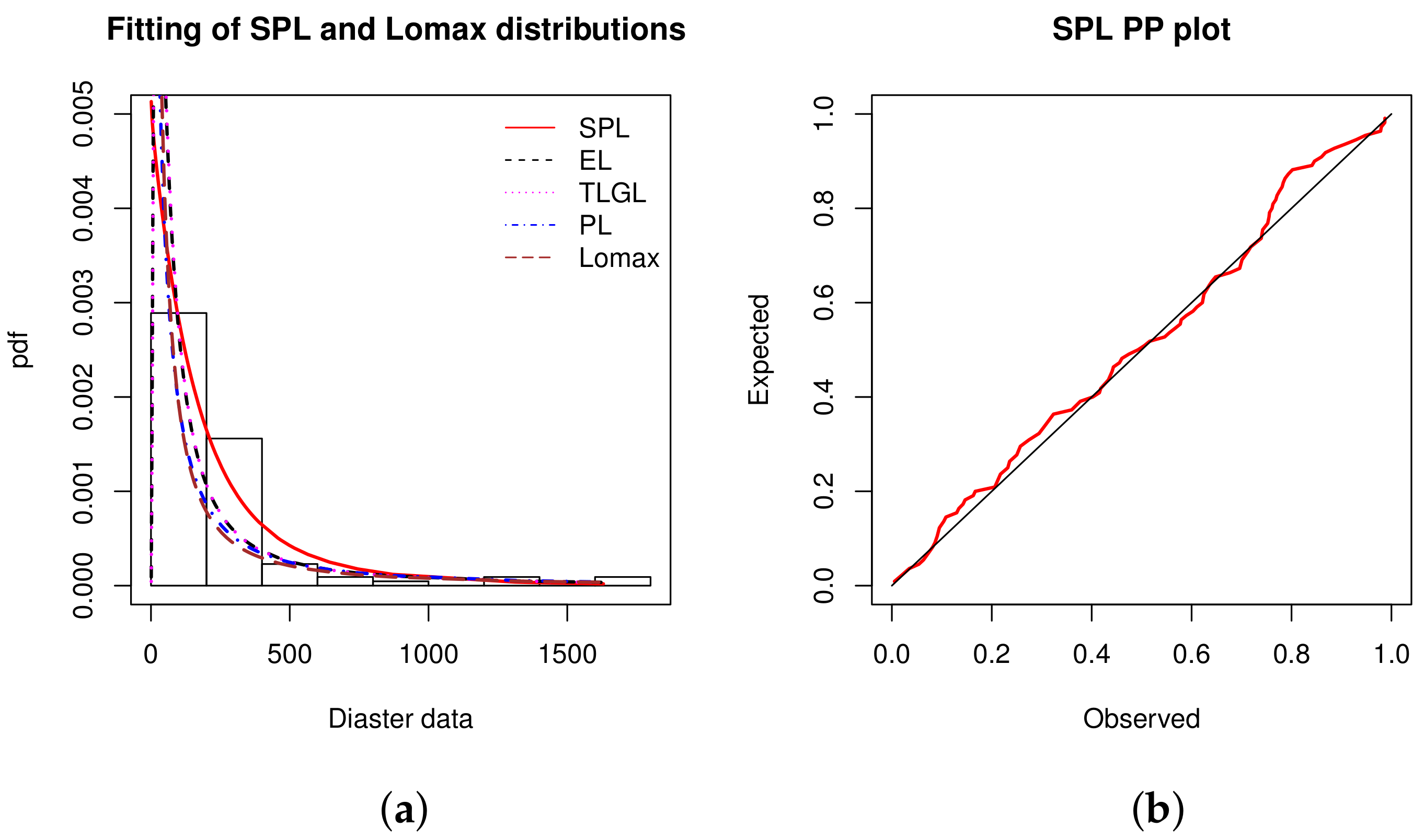
Data set 6: The data correspond to times in days between 109 successive mining catastrophes in Great Britain, for the period 1875-1951, as published in [47]. The sorted data are given as follows: 1, 4, 4, 7, 11, 13, 15, 15, 17, 18, 19, 19, 20, 20, 22, 23, 28, 29, 31, 32, 36, 37, 47, 48, 49, 50, 54, 54, 55, 59, 59, 61, 61, 66, 72, 72, 75, 78, 78, 81, 93, 96, 99, 108, 113, 114, 120, 120, 120, 123, 124, 129, 131, 137, 145, 151, 156, 171, 176, 182, 188, 189, 195, 203, 208, 215, 217, 217, 217, 224, 228, 233, 255, 271, 275, 275, 275, 286, 291, 312, 312, 312, 315, 326, 326, 329, 330, 336, 338, 345, 348, 354, 361, 364, 369, 378, 390, 457, 467, 498, 517, 566, 644, 745, 871, 1312, 1357, 1613, 1630.

A descriptive statistical summary of dataset 6 is presented in

Table 19. Descriptive statistics of dataset 6.

Mean	Median	Variance	Skewness	Kurtosis	Minimum	Maximum
233.3211	145	87873.33	2.9572	9.99439	1	1630

.

From Table 19, we can say that the data are right skewed and leptokurtic, with a very high variance.

The goodness of fit measures of the considered models are calculated and collected in

Table 20. Goodness of fit measures of the models for dataset 6.

Models	W*	A*	${\mathit{D}}_{\mathit{n}}$	p-Value	AIC	CAIC	BIC	HQIC
SPL	0.0811	0.5028	0.0646	0.7534	1407.712	1407.941	1415.786	1410.986
EL	0.5525	3.1487	0.1246	0.0679	1442.115	1442.344	1450.189	1445.389
TLGL	0.5731	3.2669	0.1300	0.0499	1443.560	1443.789	1451.634	1446.834
PL	0.2374	1.3374	0.1917	0.0006	1458.161	1458.39	1466.235	1461.436
Lomax	0.3775	2.1425	0.2114	0.0001	1463.446	1463.559	1468.829	1465.629

.

From Table 20, the SPL model shows the best results, far superior to those of the competition. The second best model is the EL model.

The MLEs of the model parameters along with their SEs are reported in

Table 21. MLEs of the model parameters for dataset 6 (in parenthesis are the SEs).

Models	$\mathit{\alpha }$	$\mathit{\beta }$	$\mathit{\lambda }$
SPL	1.667282340 (0.7019358659)	0.985393302 (0.0964258687)	0.002185021 (0.0001928461)
EL	0.7859451 (0.09768566)	11.4402958 (8.24677574)	3.8369019 (1.53466623)
TLGL	4.3433527 (3.63593087)	0.4023303 (0.07476114)	10.1888715 (15.43343884)
PL	1.0290758 (0.22032790)	0.7672704 (0.06388817)	30.6523845 (6.75638611)
Lomax	-	0.5771954 (0.07560304)	30.9556050 (6.48208435)

.

Figure 8 illustrates the nice fit of the SPL model by two different graphical approaches.

From Figure 8, we observe that the adjustment of the SPL model proposes a slope more adapted to the form of the histogram of the data, compared to those of the other models. A nice result in the PP plot is also observed.

Data set 7: The data are measures of life of Kevlar 373/epoxy fatigue fractures that are subjected to constant pressure (at the 90% stress level) until all has failed. These data was recently studied by [13] and they are: 0.0251, 0.0886, 0.0891, 0.2501, 0.3113, 0.3451, 0.4763, 0.5650, 0.5671, 0.6566, 0.6748, 0.6751, 0.6753, 0.7696, 0.8375, 0.8391, 0.8425, 0.8645, 0.8851, 0.9113, 0.9120, 0.9836, 1.0483, 1.0596, 1.0773, 1.1733, 1.2570, 1.2766, 1.2985, 1.3211, 1.3503, 1.3551, 1.4595, 1.4880, 1.5728, 1.5733, 1.7083, 1.7263, 1.7460, 1.7630, 1.7746, 1.8275, 1.8375, 1.8503, 1.8808, 1.8878, 1.8881, 1.9316, 1.9558, 2.0048, 2.0408, 2.0903, 2.1093, 2.1330, 2.2100, 2.2460, 2.2878, 2.3203, 2.3470, 2.3513, 2.4951, 2.5260, 2.9911, 3.0256, 3.2678, 3.4045, 3.4846, 3.7433, 3.7455, 3.9143, 4.8073, 5.4005, 5.4435, 5.5295, 6.5541, 9.0960.

Table 22. Descriptive statistics of dataset 7.

Mean	Median	Variance	Skewness	Kurtosis	Minimum	Maximum
1.95924	1.73615	2.47741	1.97956	5.16079	0.0251	9.096

presents a brief summary of descriptive statistics for these data.

From Table 22, it can be deduced that the data are right skewed and leptokurtic, with a low variability.

According to

Table 23. Goodness of fit measures of the models for dataset 7.

Models	W*	A*	${\mathit{D}}_{\mathit{n}}$	p-Value	AIC	CAIC	BIC	HQIC
SPL	0.0857	0.5128	0.0816	0.6620	248.7158	249.0491	255.7080	251.5102
PL	0.0924	0.5513	0.0865	0.5904	249.0608	249.3941	256.0530	251.8552
TLGL	0.1179	0.7057	0.0845	0.6184	250.9647	251.2980	257.9569	253.7591
EL	0.1183	0.7083	0.0908	0.528319	251.0226	251.3559	258.0148	253.8170
Lomax	0.1162	0.6928	0.1755	0.016153	260.8785	261.0429	265.540	262.7415

, for the purpose of optimal data fit, the SPL model is more pertinent than the other models. The second best model is the PL model.

We numerically complete the above results by showing the MLEs of the model parameters as well as the SEs in

Table 24. MLEs of the model parameters for dataset 7 (in parenthesis are the SEs).

Models	$\mathit{\alpha }$	$\mathit{\beta }$	$\mathit{\lambda }$
SPL	1.5772126 (1.0282246)	1.5747198 (0.2344551)	0.1439615 (0.1010120)
PL	3.720675 (3.720675)	1.583297 (0.2352289)	10.034301 (8.7770949)
TLGL	1.870763 (0.3248518)	6.903672 (6.2287549)	17.059630 (16.7566780)
EL	12.677044 (10.829670)	16.160300 (15.788961)	1.821291 ( 0.344925)
Lomax	-	11.57571 (6.638425)	21.51162 (13.080670)

.

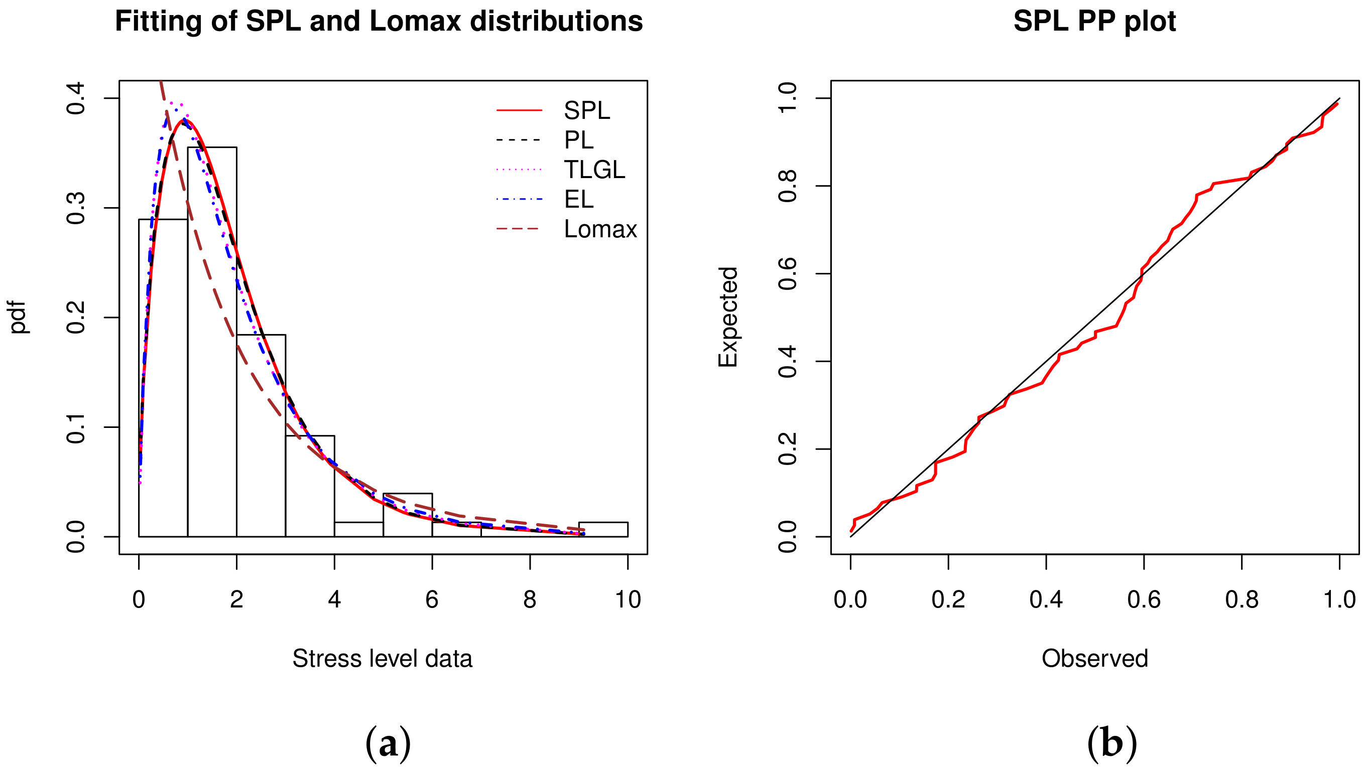
The histogram and PP plot of the data with the model fits are shown in Figure 9.

From Figure 9, in the fitting exercise, we see that the SPL model is slightly better than the competing models. A favorable PP plot is also observed.

Data set 8: Data on service times for a particular model windshield are now considered. They are given from [41]. The unit for measurement is 1000 h and the data are: 0.046, 1.436, 2.592, 0.140, 1.492, 2.600, 0.150, 1.580, 2.670, 0.248, 1.719, 2.717,0.280, 1.794, 2.819, 0.313, 1.915, 2.820, 0.389, 1.920, 2.878, 0.487, 1.963, 2.950, 0.622, 1.978, 3.003, 0.900, 2.053, 3.102, 0.952, 2.065, 3.304, 0.996, 2.117, 3.483, 1.003, 2.137, 3.500, 1.010, 2.141, 3.622, 1.085, 2.163, 3.665, 1.092, 2.183, 3.695, 1.152, 2.240, 4.015, 1.183, 2.341, 4.628, 1.244, 2.435, 4.806, 1.249, 2.464, 4.881, 1.262, 2.543, 5.140.

Table 25. Descriptive statistics of dataset 8.

Mean	Median	Variance	Skewness	Kurtosis	Minimum	Maximum
2.08527	2.065	1.55059	0.43959	−0.26741	0.046	5.14

presents a concise statistical description of these data.

We see in Table 25 that the data are right skewed and platykurtic, with a moderate variability.

Table 26. Goodness of fit measures of the models for dataset 8.

Models	W*	A*	${\mathit{D}}_{\mathit{n}}$	p-Value	AIC	CAIC	BIC	HQIC
SPL	0.1069	0.6523	0.09844	0.5418	207.4985	207.9052	213.9279	210.0272
PL	0.1479	0.9025	0.1170	0.3283	210.1077	210.5145	216.5371	212.6364
EL	0.2287	1.3837	0.1613	0.0672	214.9548	215.3616	221.3842	217.4835
TLGL	0.2473	1.4955	0.1549	0.0875	216.3146	216.7214	222.744	218.8433
Lomax	0.2211	1.3380	0.2165	0.0045	227.3478	227.5478	231.634	229.0336

indicates that the SPL model is the most appropriate fitted model. The second best model is the PL model.

Some additional elements are now given. The MLEs of the models along with their SEs are shown in

Table 27. MLEs of the model parameters for dataset 8 (in parenthesis are the SEs).

Models	$\mathit{\alpha }$	$\mathit{\beta }$	$\mathit{\lambda }$
SPL	4.98613008 (3.14343174)	1.67430554 (0.18377985)	0.02945598 (0.01925146)
PL	4.607661 (2.4059839)	1.771149 (0.1990476)	17.766353 (10.1037955)
EL	20.786925 (16.9150052)	26.841521 (21.8605907)	2.035379 (0.3637032)
TLGL	1.994239 (0.3651147)	5.493725 (3.0004375)	14.121823 (8.4044275)
Lomax	-	8.558363 (3.989779)	16.854870 (8.309326)

.

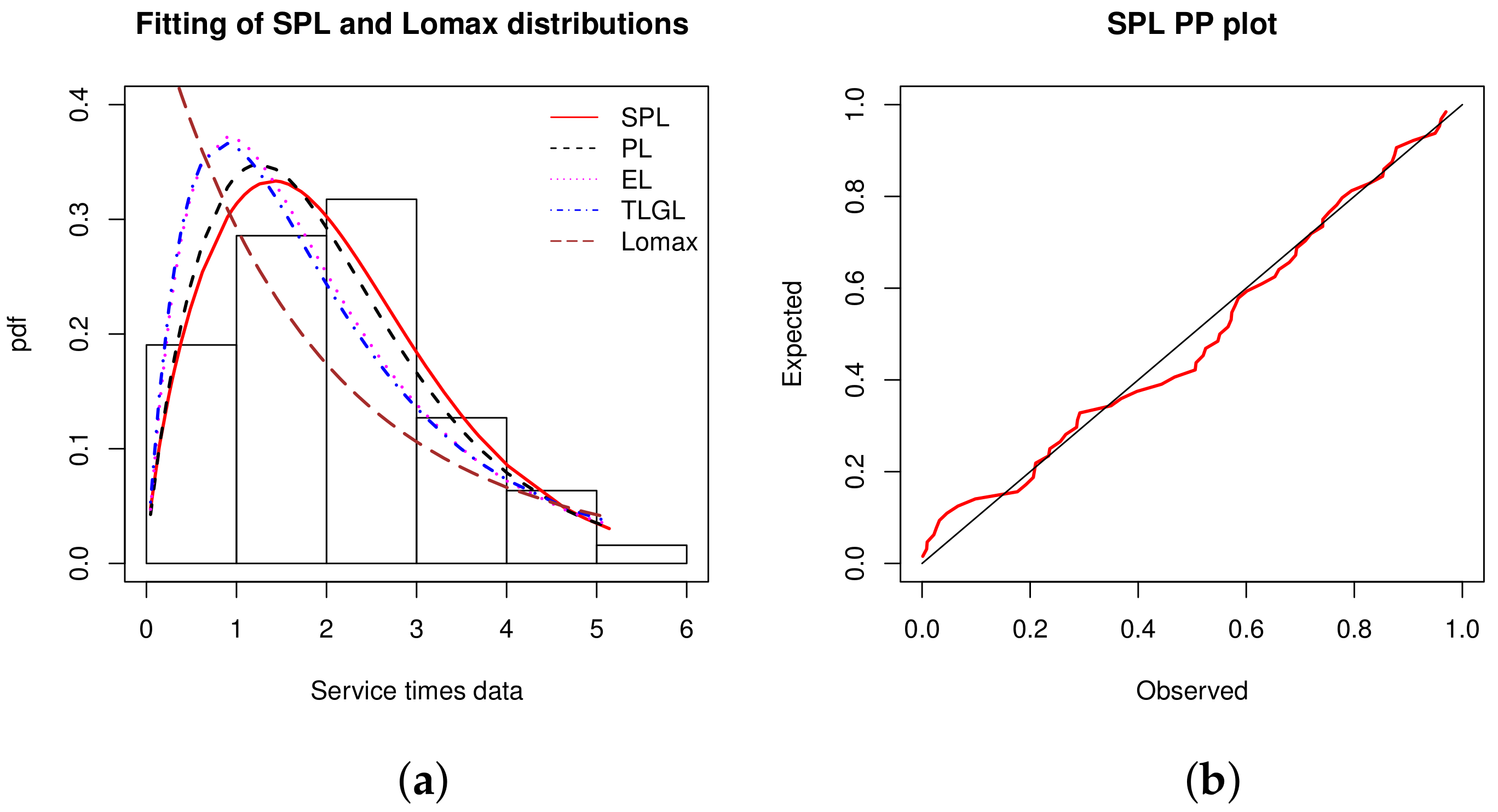
We visually see the adjustability of the SPL model in Figure 10.

From Figure 10, it is evident that the histogram of the data is better fitted by the estimated pdf of the SPL model. The red line of the PP plot is relatively close to the black line, confirming the SPL model fitting power.

Data set 9: Data relating to the strengths of 1.5 cm glass fibres which was obtained by workers at the UK National Physical Laboratory are now used. They were previously analysed by [48]. The data are: 0.55, 0.74, 0.77, 0.81, 0.84, 1.24, 0.93, 1.04, 1.11, 1.13, 1.30, 1.25, 1.27, 1.28, 1.29, 1.48, 1.36, 1.39, 1.42, 1.48, 1.51, 1.49, 1.49, 1.50, 1.50, 1.55, 1.52, 1.53, 1.54, 1.55, 1.61, 1.58, 1.59, 1.60, 1.61, 1.63, 1.61, 1.61, 1.62, 1.62, 1.67, 1.64, 1.66, 1.66, 1.66, 1.70, 1.68, 1.68, 1.69, 1.70, 1.78, 1.73, 1.76, 1.76, 1.77, 1.89, 1.81, 1.82, 1.84, 1.84, 2.00, 2.01, 2.24.

A first statistical approach of these data is proposed in

Table 28. Descriptive statistics of dataset 9.

Mean	Median	Variance	Skewness	Kurtosis	Minimum	Maximum
1.50683	1.59	0.10506	−0.89993	0.92376	0.55	2.24

.

From Table 28, we observe that the data are left skewed and platykurtic, with almost negligible dispersion.

The goodness of fit measures of the considered models are calculated and collected in

Table 29. Goodness of fit measures of the models for dataset 9.

Models	W*	A*	${\mathit{D}}_{\mathit{n}}$	p-Value	AIC	CAIC	BIC	HQIC
SPL	0.2637	1.4444	0.1639	0.0678	36.95819	37.36497	43.38759	39.4869
PL	0.4157	2.2916	0.2232	0.0038	46.09434	46.50112	52.52375	48.62306
TLGL	0.8017	4.3691	0.2258	0.0032	70.44963	70.85641	76.87904	72.97835
EL	0.8222	4.4767	0.2263	0.0031	71.82442	72.2312	78.25382	74.35313
Lomax	0.5854	3.2101	0.4210	3.98$\times {10}^{-10}$	186.006	186.206	190.2923	187.6918

.

According to Table 29, we assert that the SPL model has a better goodness of fit than the other models. The second best model is the PL model.

The MLEs of the model parameters and their SEs are shown in

Table 30. MLEs of the model parameters for dataset 9 (in parenthesis are the SEs).

Models	$\mathit{\alpha }$	$\mathit{\beta }$	$\mathit{\lambda }$
SPL	3.02842979 (1.619006155)	5.77611926 (0.666909675)	0.01281263 (0.007095599)
PL	1.945485 (0.6988577)	6.010487 (0.7239624)	23.913933 (8.2279128)
TLGL	32.13406 (10.38371)	24.84223 (19.00308)	18.21983 (14.95689)
EL	27.01510 (15.272308)	9.35084 (5.989516)	35.10721 (11.975072)
Lomax	-	13.77391 (6.867307)	19.96670 (9.995415)

.

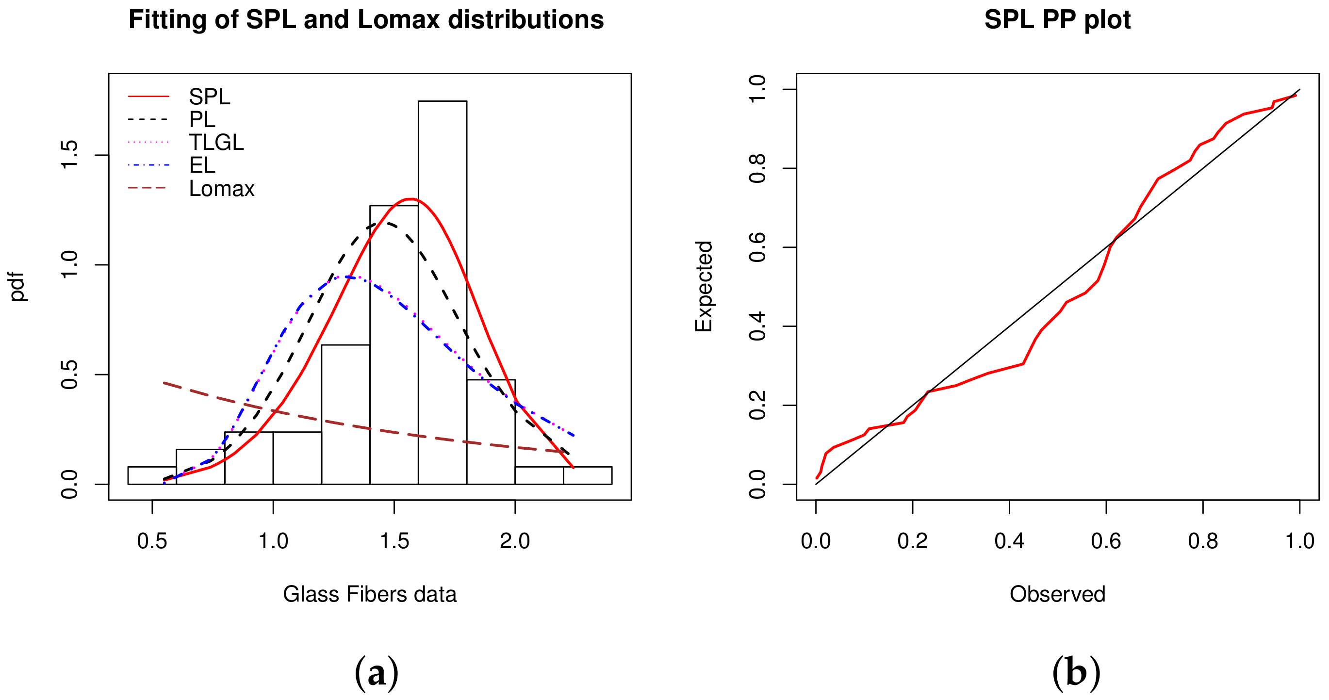
Estimated pdfs over the histogram of the data and PP plot of the SPL model are shown in Figure 11.

From Figure 11, unsurprisingly in view of Table 30, the SPL model shows the best fit curve of the histogram. A nice fit of the SPL model is also validated by the PP plot.

5. Conclusions

The main contribution of the article is to propose a new efficient statistical modelling strategy through a flexible trigonometric extension of the famous power Lomax model. In this regard, we use the functionalities of the sine generalized (S-G) family of distributions and introduce the sine power Lomax (SPL) distribution. We exhibited some of its interesting characteristics, with an emphasis on the modelling ability of the corresponding probability density and hazard rate functions, and discussed the moments and incomplete moments. Simulations and applications illustrate the usefulness of the considered SPL model. In particular, we carried out nine practical datasets for the evaluation of the SPL model with the main existing models derived from the Lomax model. Whenever the data is symmetric or skewed, the SPL model performs better than the competing models considered. Thus, the results obtained are quite satisfactory, showing that the SPL model can be used fairly to efficiently analyse a large panel of datasets.

References

- Freedman, D.A. Statistical Models: Theory and Practice; Cambridge University Press: Cambridge, UK, 2005; ISBN 978-0-521-67105-7. [Google Scholar]
- McCullagh, P. What is a statistical model ? Ann. Stat. 2002, 30, 1225–1310. [Google Scholar] [CrossRef]
- Brito, C.R.; Rêgo, L.C.; Oliveira, W.R.; Gomes-Silva, F. Method for generating distributions and classes of probability distributions: The univariate case. Hacet. J. Math. Stat. 2019, 48, 897–930. [Google Scholar]
- Kumar, D.; Singh, U.; Singh, S.K. A new distribution using sine function: its application to bladder cancer patients data. J. Stat. Appl. Probab. 2015, 4, 417–427. [Google Scholar]
- Souza, L. New Trigonometric Classes of Probabilistic Distributions. Ph.D. Thesis, Universidade Federal Rural de Pernambuco, Recife, Brazil, 2015. [Google Scholar]
- Souza, L.; Junior, W.R.O.; de Brito, C.C.R.; Chesneau, C.; Ferreira, T.A.E.; Soares, L. On the Sin-G class of distributions: theory, model and application. J. Math. Model. 2019, 7, 357–379. [Google Scholar]
- Souza, L.; Junior, W.R.O.; de Brito, C.C.R.; Chesneau, C.; Ferreira, T.A.E.; Soares, L. General properties for the Cos-G class of distributions with applications. Eurasian Bull. Math. 2019, 2, 63–79. [Google Scholar]
- Lee, C.; Famoye, F.; Olumolade, O. Beta-Weibull distribution: Some properties and applications to censored data. J. Mod. Appl. Stat. Methods 2007, 6, 173–186. [Google Scholar] [CrossRef]
- Nelson, W. Applied Life Data Analysis; John Wiley and Sons: New York, NY, USA, 1982. [Google Scholar]
- Bjerkedal, T. Acquisition of resistance in guinea pigs infected with different doses of virulent tubercle bacilli. Am. J. Hyg. 1960, 72, 130–148. [Google Scholar]
- Souza, L.; Gallindo, L.; Serafim-de-Souza, L. SinIW: The SinIW Distribution. R Package Version 0.2. 2016. Available online: https://CRAN.R-project.org/package=SinIW (accessed on 2 February 2021).
- Chesneau, C.; Bakouch, H.S.; Hussain, T. A new class of probability distributions via cosine and sine functions with applications. Commun. Stat. Simul. Comput. 2019, 48, 2287–2300. [Google Scholar] [CrossRef]
- Jamal, F.; Chesneau, C. A new family of polyno-expo-trigonometric distributions with applications, Infinite Dimensional Analysis. Quantum Probab. Relat. Top. 2019, 22, 1950027. [Google Scholar] [CrossRef] [Green Version]
- Mahmood, Z.; Chesneau, C.; Tahir, M.H. A new sine-G family of distributions: properties and applications. Bull. Comput. Appl. Math. 2019, 7, 53–81. [Google Scholar]
- Al-Babtain, A.A.; Elbatal, I.; Chesneau, C.; Elgarhy, M. Sine Topp-Leone-G family of distributions: Theory and applications. Open Phys. 2020, 18, 574–593. [Google Scholar] [CrossRef]
- Jamal, F.; Chesneau, C. The sine Kumaraswamy-G family of distributions. J. Math. Ext. 2021, in press. [Google Scholar]
- Rady, E.H.A.; Hassanein, W.A.; Elhaddad, T.A. The power Lomax distribution with an application to bladder cancer data. SpringerPlus 2016, 5, 1–22. [Google Scholar] [CrossRef] [PubMed] [Green Version]
- Lomax, K.S. Business Failures; Another example of the analysis of failure data. J. Am. Stat. Assoc. 1954, 49, 847–852. [Google Scholar] [CrossRef]
- Johnson, N.L.; Kotz, S.; Balakrishnan, N. Continuous Univariate Distributions 1, 2nd ed.; Wiley: New York, NY, USA, 1994. [Google Scholar]
- Abdullah, M.A.; Abdullah, H.A. Estimation of Lomax parameters based on generalized probability weighted moment. J. King Abdulaziz Univ. Sci. 2010, 22, 171–184. [Google Scholar]
- Afaq, A.; Ahmad, S.P.; Ahmed, A. Bayesian Analysis of shape parameter of Lomax distribution under different loss functions. Int. J. Stat. Math. 2010, 2, 55–65. [Google Scholar]
- Ahsanullah, M. Record values of Lomax distribution. Stat. Ned. 1991, 41, 21–29. [Google Scholar] [CrossRef]
- Balakrishnan, N.; Ahsanullah, M. Relations for single and product moments of record values from Lomax distribution. Sankhya B 1994, 56, 140–146. [Google Scholar]
- Balkema, A.; de Haan, L. Residual life time at great age. Ann. Probability 1974, 2, 792–804. [Google Scholar] [CrossRef]
- Bryson, M.C. Heavy-tailed distributions: properties and tests. Technometrics 1974, 16, 61–68. [Google Scholar] [CrossRef]
- Ferreira, P.H.; Ramos, E.; Ramos, P.L.; Gonzales, J.F.B.; Tomazella, V.L.D.; Ehlers, R.S.; Silva, E.B.; Louzada, F. Objective Bayesian analysis for the Lomax distribution. Stat. Probab. Lett. 2020, 159, 108677. [Google Scholar] [CrossRef] [Green Version]
- Al-Marzouki, S.; Jamal, F.; Chesneau, C.; Elgarhy, M. Type II Topp Leone power Lomax distribution with applications. Mathematics 2020, 8, 4. [Google Scholar] [CrossRef] [Green Version]
- Fayomi, A. Type I half logistic power Lomax distribution: Statistical properties and application. Adv. Appl. Stat. 2019, 54, 85–98. [Google Scholar] [CrossRef]
- Hassan, A.S.; Abd-Allah, M. On the inverse power Lomax distribution. Ann. Data Sci. 2019, 6, 259–278. [Google Scholar] [CrossRef]
- Haq, M.A.; Srinivasa-Rao, G.; Albassam, M.; Aslam, M. Marshall-Olkin power lomax distribution for modeling of wind speed data. Energy Rep. 2020, 6, 1118–1123. [Google Scholar] [CrossRef]
- Abd El-Monsef, M.M.E.; Sweilam, N.H.; Sabry, M.A. The exponentiated power Lomax distribution and its applications. Qual. Reliab. Eng. Int. 2021. [Google Scholar] [CrossRef]
- Nagarjuna, V.B.V.; Vardhan, R.V.; Chesneau, C. Kumaraswamy generalized power Lomax distribution and its applications. Stats 2021, 4, 28–45. [Google Scholar] [CrossRef]
- Nair, N.U.; Sankaran, P.; Balakrishnan, N. Quantile-Based Reliability Analysis; Birkhäuser: Basel, Switzerland, 2013. [Google Scholar]
- Cordeiro, G.M.; Silva, R.B.; Nascimento, A.D.C. Recent Advances in Lifetime and Reliability Models; Bentham Books: Sharjah, United Arab Emirates, 2020. [Google Scholar]
- Casella, G.; Berger, R.L. Statistical Inference; Duxbury Advanced Series Thomson Learning: Pacific Grove, CA, USA, 2002. [Google Scholar]
- R Development Core Team. R: A Language and Environment for Statistical Computing; R Foundation for Statistical Computing: Vienna, Austria, 2005; ISBN 3-900051-07-0. [Google Scholar]
- Konishi, S.; Kitagawa, G. Information Criteria and Statistical Modeling; Springer: New York, NY, USA, 2007. [Google Scholar]
- Oguntunde, P.E.; Khaleel, M.A.; Okagbue, H.I.; Odetunmibi, O.A. The Topp-Leone lomax (TLLO) distribution with applications to airbone communication transceiver dataset. Wirel. Pers. Commun. 2019, 109, 349–360. [Google Scholar] [CrossRef]
- Lemonte, A.J.; Cordeiro, G.M. An extended Lomax distribution. Statistics 2013, 47, 800–816. [Google Scholar] [CrossRef]
- Lee, E.T.; Wang, J.W. Statistical Methods for Survival Data Analysis; Wiley: New York, NY, USA, 2003. [Google Scholar] [CrossRef]
- Murthy, D.N.P.; Xie, M.; Jiang, R. Weibull Models; John Wiley and Sons: New York, NY, USA, 2004. [Google Scholar]
- Silva, R.V.; Silva, F.G.; Ramos, M.W.A.; Cordeiro, G.M. A new extended gamma generalized model. Int. J. Pure Appl. Math. 2015, 100, 309–335. [Google Scholar] [CrossRef] [Green Version]
- Proschan, F. Theoretical explanation of observed decreasing failure rate. Technometrics 1963, 5, 375–383. [Google Scholar] [CrossRef]
- Lorenzo, E.; Malla, G.; Mukerjee, H. A new test for decreasing mean residual lifetimes. Commun. Stat. Theory Methods 2018, 47, 2805–2812. [Google Scholar] [CrossRef]
- Bader, M.; Priest, A. Statistical aspects of fibre and bundle strength in hybrid composites. In Progress in Science and Engineering Composites; Hayashi, T., Kawata, K., Umekawa, S., Eds.; ICCM-IV: Tokyo, Japan, 1982; pp. 1129–1136. [Google Scholar]
- Nichols, M.D.; Padgett, W.J. A bootstrap control chart for Weibull percentiles. Qual. Reliab. Eng. Int. 2006, 22, 141–151. [Google Scholar] [CrossRef]
- Maguire, B.A.; Pearson, E.; Wynn, A. The time intervals between industrial accidents. Biometrika 1952, 39, 168–180. [Google Scholar] [CrossRef]
- Smith, R.L.; Naylor, J.C. A comparison of maximum likelihood and bayesian estimators for the three-parameter weibull distribution. Appl. Stat. 1987, 36, 258–369. [Google Scholar] [CrossRef]
Figure 1.
Curves of the pdf of the SPL distribution at different parameter values.
Figure 2.
Curves of the hrf of the SPL distribution at different parameter values.
Figure 3.
(a) Plot of the estimated pdfs over the histogram and (b) PP plot of the SPL model for dataset 1.
Figure 4.
(a) Plot of the estimated pdfs over the histogram and (b) PP plot of the SPL model for dataset 2.
Figure 5.
(a) Plot of the estimated pdfs over the histogram and (b) PP plot of the SPL model for dataset 3.
Figure 6.
(a) Plot of the estimated pdfs over the histogram and (b) PP plot of the SPL model for dataset 4.
Figure 7.
(a) Plot of the estimated pdfs over the histogram and (b) PP plot of the SPL model for dataset 5.
Figure 8.
(a) Plot of the estimated pdfs over the histogram and (b) PP plot of the SPL model for dataset 6.
Figure 9.
(a) Plot of the estimated pdfs over the histogram and (b) PP plot of the SPL model for dataset 7.
Figure 10.
(a) Plot of the estimated pdfs over the histogram and (b) PP plot of the SPL model for dataset 8.
Figure 11.
(a) Plot of the estimated pdfs over the histogram and (b) PP plot of the SPL model for dataset 9.