
Admission Control in Home Energy Management Systems Using Theatre and Hybrid Actors


1
ICAR-CNR, 87036 Rende, CS, Italy
2
DIMES-UNICAL, 87036 Rende, CS, Italy
*
Author to whom correspondence should be addressed.
Modelling 2021, 2(2), 288-307; https://0-doi-org.brum.beds.ac.uk/10.3390/modelling2020015
Submission received: 25 March 2021
/
Revised: 29 April 2021
/
Accepted: 10 May 2021
/
Published: 12 May 2021
Abstract
:The goal of a Home Energy Management System (HEMS) is that of purposely shaping the cumulative energy consumption curves of domestic appliances by imposing suitable monitoring and control policies. The development of HEMS, like the development of general Cyber-Physical Systems (CPSs), is challenging, as it requires the exploitation of suitable methodological approaches which are able to deal jointly with the continuous and discrete behaviours of a CPS. In this paper, a methodological approach for HEMS is advocated which relies on the use of the Theatre actor system with hybrid actors. As a key feature, Theatre enables the same actor model to be used during the analysis, design, prototyping and implementation phases of the system. For property assessment, a Theatre model is reduced to Uppaal hybrid timed automata for analysis by statistical model checking. As a significant modelling example, a HEMS is proposed which implements an admission control strategy able to maintain the in-home energy consumption under a given threshold. Instead of reacting to an overload condition, the strategy is able to prevent an overload upfront by predicting the effect that the admission of a new load will have on the consumption curve of the whole system.
1. Introduction
Nowadays, there are many research efforts addressing issues tied to the production, distribution and consumption of electrical energy. Many such efforts are directed to make energy utilization as efficient as possible, so as to promote environmental and economic sustainability [1,2,3,4]. The cost-reduction of IoT-based smart appliances and their pervasive diffusion favours the exploitation of efficient energy management strategies also in a domestic context [3,4]. A Home Energy Management System (HEMS) [3,5] is a Cyber-Physical System (CPS) for monitoring and management of in-home appliances with the goal of shaping the overall energy consumption curve by imposing a proper load scheduling policy.
Load scheduling is a multifaceted problem [3,4,6,7,8]. In a case, the goal could be that of promoting the reduction of energy consumption by the automatic scheduling of loads and by also providing feedback to customers for encouraging a more efficient use of electricity [8]. Comfort issues are considered in [7]. The performance of some scheduling algorithms is studied in [3] and the demand in terms of computational resources and the complexity of the required execution infrastructure are considered for assessing the performance. The automatic identification of plugged appliances is the goal of the work described in [9]. Privacy concerns in managing consumption profiles of the users are instead considered in [4].
While designing and implementing a HEMS, some important issues need to be taken into account. Some of them, tied to the development of CPSs in general, are: (i) guaranteeing a right coupling between the discrete dynamics of the cyber-part of the system with the continuous behaviour (i.e., the modes of the system) of the physical environment in which the CPS operates. For these purposes, approaches and methodologies related to hybrid systems need to be used; (ii) assessing functional and timing properties of the system; (iii) adopting a development process that helps to transfer the validity of the analysed properties into the final system implementation; (iv) handling concurrency problems carefully.
Despite their importance, though, the above issues are often not adequately supported in today’s computing and networking infrastructures, and no widely-used programming languages are capable of natively dealing with temporal properties [10].
In this paper, the Theatre infrastructure [11] enriched with hybrid actors [12] is advocated since they offer a modelling and development approach suited to cope with the problems so far discussed. A theatre is the runtime environment for actors. An actor is a software component (agent) which shares no data and communicates with other actors by exchanging asynchronous messages. Actors support a cooperative model of concurrency that simplifies the development of distributed/concurrent applications and avoid coping with common pitfalls of multi-threaded programming [13]. They are smart agents [14] having the ability to migrate dynamically from a computing node to another, thus possibly moving an intelligent behaviour close to the devices they have to interact with.
Hybrid actors naturally exhibit a time-dependent behaviour, and rely on the use of continuous modes thus permitting to model the dynamic behaviours of a CPS. Theatre and actors favour model continuity [15,16], that is the possibility of transitioning an actor model throughout the whole life-cycle of a system, from analysis down-to design, implementation and real execution. Property assessment is achieved by mapping a hybrid Theatre model onto hybrid timed automata for statistical model checking [17] in the context of the popular Uppaal toolbox [18].
The contribution of this work is threefold: (i) the definition of an approach capable of revealing some desired/undesired properties emerging when coupling the cyber with the physical part of a CPS; (ii) the use of Theatre with hybrid actors in the case what-if scenarios are required to be evaluated and continuous behaviours require to be suspended and (subsequently) resumed; (iii) the exploitation of the approach in a significant modelling example related to the context of home energy management.
With respect to previous authors’ works [19,20], this paper proposes a load scheduling strategy for HEMS relying on a prediction-based admission control policy [5]. More in particular, instead of reacting to an overload condition, the strategy prevents an overload upfront by predicting the effects that the admission of a new load will have on the consumption curve of the whole HEMS. Consumption curves, both real and predicted, of the considered appliances are specified by Ordinary Differential Equations (ODEs).
The structure of the paper is as follows. Section 2 summarizes some related works; Section 3 describes the HEMS chosen as a case study; Section 4 describes basic concepts concerning an actor-based design of CPSs and the use of the Uppaal timed automata for modelling and analysis purposes; Section 5 details the achieved model for the HEMS; Section 6 shows some experimental results related to property checking; finally, Section 7 concludes the paper and gives some indications about on-going and future work.
2. Related Work
This paper proposes an original approach here used for modelling and analysing home energy management systems which is based on the use of time-sensitive actors in the context of the Theatre architecture and framework [11,12]. Actors [21] are highly-modular, concurrent and distributed software entities. They share no data and communicate with each other by asynchronous message passing. The Actor model born as a formalism well-suited to the development of untimed applications tolerating non-determinism in the message processing. Some variants of actors, though, have been proposed with the goal of addressing real-time constraints and enabling, in some cases, repeatability in the model execution by enforcing an ordered message delivery.
In [22], the proposed actor model relies on reactors which favour system composability by interconnecting typed input/output ports carrying events (messages). The behaviour of reactors is specified by reactions, which are message handler methods that can modify local data status and act as input/output event transformers. Timing aspects are managed through timers triggering reactions at selected times, and by delays and deadlines in reactors, which, respectively, constrain the generation of an output event or specify a time limit on the delivery of an event. Reactors rest on time-stamped messages. Reactors are part of the current meta-modelling polyglot language named Lingua Franca [23], which permits to specify the reactions’ body in various languages like C, Python, and Java.
Other timed actor-based modelling and implementation languages, like Timed Rebeca [24] and Theatre [14], also rely on concepts borrowed from Reactors. In Timed Rebeca, an actor (rebec) owns an internal thread. Two attributes, namely after and deadline, can be attached to messages so as to specify, respectively, the time which has to pass before the message can be consigned, and the maximum allowed amount of time within which the message should be delivered. A message is discarded in the case its deadline expires. Timed Rebeca exploits a suspensive execution model for reactions (called message servers), in which a delay statement can be used to specify the duration of a code fragment. A model defined in Lingua Franca can be transformed into Timed Rebeca [23] for model checking by using the Afra tool. Theatre (see Section 4) syntactically resembles Timed Rebeca. However, a Theatre model (i) is composed of lightweight actors (they have no internal thread); (ii) actors have message reactions with non-suspensive semantics; and (iii) message scheduling and ordered delivery is regulated by a customizable control strategy. The possibility of exhaustive model checking CPS models based on a deterministic version of Theatre, when arbitrary continuous behaviour in peripheral entities is relaxed, is shown in [25].
Due to the ever-increasing demand for electric energy and to the availability of renewable power sources near to the utilization site (like photovoltaic panels and wind turbines), a great interest has grown in optimizing energy consumption also in domestic smart environments [9]. A HEMS is devoted to shaping the consumption curves of intelligent appliances, e.g., through the use of smart plugs, so as to impose suitable scheduling strategies with the goal of keeping the desirable overall power consumption under a given threshold.
Devising effective scheduling algorithms for electric loads is a multifaceted and challenging problem [3,4,6,7,8]. In many cases, a trade-off between energy consumption and the comfort level of the occupants is required to be considered. In [7], an adaptive algorithm devoted to reducing energy consumption without degrading the comfort level perceived by the home occupants is proposed. Deep Reinforcement Learning is used in [8] for on-line load scheduling optimization in a smart grid context. Here, in order to favour a more efficient use of electricity, the scheduling algorithm also provides the customer with some feedback in real-time. The use of different centralized and decentralized scheduling algorithms is instead provided in [3]. The main goal is that of helping customers in modifying their consumption patterns. Furthermore, the above paper compares some scheduling algorithms on the basis of the amount of needed resources and the complexity of the required runtime infrastructure. The work presented in [9] discusses a different issue that is tied to the automatic identification of an electric load after it is plugged into the energy management system. The minimization of the electricity bill is fostered in [26], where renewable energy sources are taken into account within a load scheduling strategy based on reinforcement learning. A Q-learning based approach for optimizing energy consumption which also admits variable consumers’ habits and a variable energy price is proposed in [27]. The approach does not consider variable profiles for load consumption and self-produced energy. The problem of preserving privacy while managing people profiles is instead taken into account in [4].
The actor-based approach proposed in this paper is powerful and flexible, allows a formal modelling of an energy management system like scheduling appliances in a smart home so as to reduce the electricity costs, and enables a thorough evaluation of model properties before transitioning the model to final synthesis and implementation.
3. A Home Energy Management System
A HEMS is a CPS devoted to automatically monitoring and managing the operations of in-home appliances. The goal is to enforce control policies able to shape the overall power/energy consumption curves [3,5,16,28,29]. For this purpose, many different techniques can be purposely used. For instance, a load shedding/shifting approach can be exploited in the case the total power consumption exceeds a given threshold [3,29].
The HEMS here proposed adopts an admission control policy on incoming loads which detects and prevents overload upfront [5]. Specifically, the proposed control policy is able to avoid that the admission of a new load could cause, in the future, the exceeding of a given consumption threshold. The approach, though, is more general and can be used, e.g., to ensure that the overall consumption curve of the system will own some specific features and properties without resorting to recovery operations.
Proposed approach permits to deal with a general challenge arising when developing CPSs which is to establish a proper sampling frequency for sensing the physical environments. This is an important precondition in order to properly couple the cyber and the physical part of the system. According to the well-known sampling theorem, the sampling frequency determines “the view” that the cyber component has of the physical one. Obviously, down-sampling the environment leads to a partial, yet distorted, vision of the physical world. Over-sampling the environment, instead, can be useless and resource-wasting. From a practical point-of-view it is important to chose the right (minimum) sampling frequency that permits the CPS to properly behave, and to determine how the system behaves when such frequency varies.
The chosen HEMS consists of a set of remote controllable smart plugs, a controller, and an energy meter. The meter is used to sample the actual consumption curves of the loads and to provide such information to the controller. By varying the frequency with which the meter sends a sample to the controller, it is possible to change the view that the controller has about the whole system.
Appliances can be dynamically plugged or removed, and the controller is used to determine if an incoming new load can be really activated or it must be deferred. A load is activated if its power consumption curve summed to the cumulative consumption curves of the already active loads will keep the future total requested power under a given threshold. In order to check this property, each load is able to furnish a prediction about its remaining/future power demand. As soon as a new load announces itself, the controller switches the HEMS into a prediction mode in which each load stops its execution and starts to furnish its future predicted power consumption. After the prediction phase, the controller will switch-back the system into the normal operational mode and will activate the incoming load only in the case that the threshold is not violated during the prediction. In the case where a violation emerges, the not-admissible load is added to a deferred-load set and, after a given timeout, the controller will again try to admit one of the loads in the waiting set by again checking violations on the threshold through prediction. Both in the operational and prediction modes, all the appliances evolve according to their known continuous behaviours, which are modelled through ODEs. The challenge here is that of: (i) suddenly freezing the evolution of all the continuous behaviours tied to the operating components as soon as a new load announce itself; (ii) evaluating how the system would evolve if the new load is added to the already operating loads and checking for threshold violations; (iii) restarting all the frozen continuous behaviour by resuming them from the exact point they were suspended and, if no violations occurred, making operating the new load.
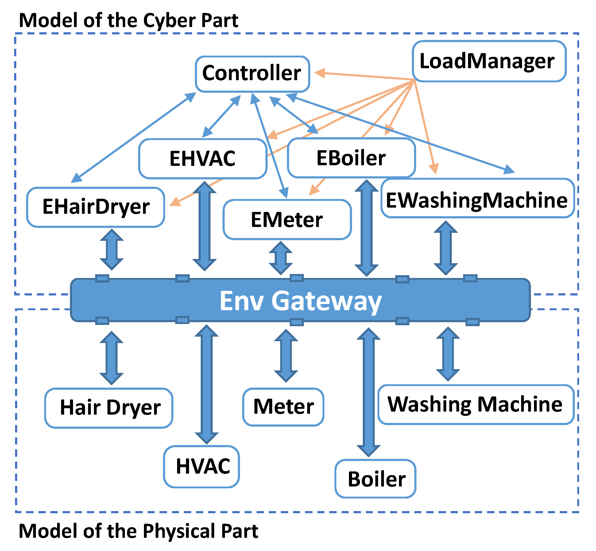
The architecture of the considered HEMS is depicted in Figure 1. The system is made of two main parts: the cyber part, whose components implement the application logic of the HEMS, and the physical part whose components are place holders of the real equipment. The cyber part contains the Controller, the EMeter, the LoadManager and four load components, namely, EHairDryer, EHVAC, EWashingMachine, and EBoiler, which manage the components in the physical part. The prefix E means enhanced. This is because such components enhance the functionalities of the managed real equipment by adding the prediction abilities required by the controller. The LoadManager is in charge of configuring and starting the system. The EnvGateway [16], is a boundary element permitting a transparent interaction between the cyber and the physical part. When the HEMS moves from the analysis to the implementation phase, the components into the physical part are replaced by real hardware components and only the EnvGateway will be affected by this change, all the other cyber components remain unaware of this phase transition. Communication patterns existing among components are highlighted in Figure 1 by using mono-directional and bidirectional arrows.
The consumption curves of the enhanced loads are reported in Figure 2. The red part of a curve represents the real power consumption. The light-blue part, instead, represents the consumption during the prediction phase. The curves are modelled and obtained by using continuous modes. Each load has its own specific continuous modes. To prevent visualization clutter, the prediction curves are purposely drawn by considering negative values. As a consequence, a prediction and a real curve of a given load will have the same shape but opposite sign. It is the responsibility of an enhanced load to furnish the proper kind of consumption curve on the base of its working state. Three working states are admitted, namely:
- Active: The load is operating and consumes real power. In this state, the time of the load evolves as the load performs its operation.
- Coasting Forward: The load is not operating and the time of the load gets frozen, i.e., it does not evolve. This phase is preparatory to the prediction state. Since the evolution of the consumption curves during prediction must start from the exact instant in which the load stopped to be active, a coasting forward phase is required to ensure that the prediction curve, starting from the beginning, reaches this instant. In the case a load was not yet activated, during the coasting forward, no operations are carried out.
- Prediction: The load is not operating but the time of the load evolves according to a virtual time notion exploited only for prediction purposes. Once started, the prediction phase runs to completion.
From the above description, it follows that in Figure 2 two time notions are exploited on the x-axis of each consumption curve: a virtual time notion for the prediction and an operating time notion representing the evolution of the activities carried out by the load.
The controller regulates the state transitions of the loads and enforces that all the loads stay in “coherent states”. For instance, considering the scenario in which all the admitted loads are Active, on receiving an admission request from a new load, the controller suspends the active loads by turning them into Coasting Forward. As soon as all the loads completed the coasting forward, the controller switches the loads into Prediction and starts to monitor the predicted power in order to evaluate threshold violations. At the end of the prediction phase, the previously-suspended loads are turned again into Active and their operations are resumed. The new load is switched to Active if and only if no threshold violations occurred during prediction, otherwise the admission of the new load is deferred by the controller. This approach permits any load to be suspended and resumed whenever it is needed, and a new load can announce itself at any time.
The above-described components coordinate with each other by exploiting a purposely designed message interface. The messages exchanged in the system are reported in Table 1. For each message, the message name, a description, and the components using it are specified.
4. Modelling Using Actors and Uppaal
The Theatre actor-based modelling language [11,30] and Java software framework [25] are chosen in this work for the development of time-critical cyber–physical systems [16]. The following summarizes the fundamental concepts of Theatre.
4.1. Basic Issues of Theatre
A Theatre is a federation of computing nodes (theatres/JVMs), connected to each other by network services (e.g., based on TCP sockets). A theatre hosts a collection of actors together with a transparent and customizable reflective control layer, i.e., the control machine, having the responsibility of regulating the scheduling and dispatching of messages. An actor is a modular entity encapsulating a data status. Communication among actors relies on asynchronous message passing. Differently from classical actor systems [21,24], Theatre actors are without threads. An actor is at rest until a message arrives. Message processing is atomic and cannot be suspended nor pre-empted. Actors do not have a local message mailbox, they depend on the buffering and time management services offered by the local control machine. The various control machines coordinate with each other in a distributed fashion so as to keep aligned, through the mediation of a time server [16], a notion of global time (real-time or simulated-time). The macro-step semantics [31] holds within a same theatre: the dispatch of each message runs to completion before a further message gets selected and dispatched. By default, the time needed for message processing is assumed to be negligible. In this way, a cooperative form of concurrency is obtained in a theatre by message interleaving, thus favouring time-predictability. True parallelism occurs among actors allocated on distinct theatres.
A Theatre model [11] can be abstracted by a set of processing units (PUs/theatres) and the actors can be allocated to PUs by means of the move(act,pu) operation. An actor class consists of hidden local variables, including acquaintance actors to which messages can be sent, plus an interface of message servers (msgsrv) [24]. A msgsrv is a void method which can have arguments. It is devoted to processing an homonymous message. The body of a msgsrv is a block of instructions which includes assignment, if-then-else, send and delay operations. The instruction dest.send( msgsrv-name[, args] ) [after] [deadline] sends asynchronously to the dest actor a request to execute a given msgsrv. The optional after and deadline time attributes are relative to the sending time and, respectively, specify that the message cannot be delivered before after time units are elapsed, and that, would time go beyond the deadline, the message loses its validity and needs to be discarded. The default values for after and deadline are, respectively, 0 and ∞. The duration of a msgsrv can be specified through a delay(d) operation. If used, delay must be the last operation of a msgsrv.
The semantics of a Theatre model [11] can be formally specified as a timed transition system in which each state is composed of (a) the current value of the global time (now), (b) the union of all the actor data statuses, (c) the bag of the already sent but not yet dispatched messages, (d) the bag of the already set but not yet expired delays. Two types of transitions exist: (i) a time transition which advances the global time to the occurrence time of the most imminent event (message dispatch or delay expiration), (ii) an action transition which specifies either the execution of a message server (message dispatch) or a delay expiration (which makes free a given PU). If multiple events occur at the same time, one of them is chosen not-deterministically.
4.2. Introducing Hybrid Actors
The basic version of Theatre is extended so as to be more apt for CPSs. CPSs need, during analysis, a proper modelling of the continuous behaviour of the external environment of the physical part, to be integrated with the (event and time) discrete behaviour of the cyber part. For this reason, the notion of continuous mode was added by following the concepts of hybrid automata [12,33]. Differently from [12], continuous modes are considered as independent components which are modelled externally to the application actors, and that naturally can execute in parallel.
A continuous mode is activated by an actor (called accessor in [34]). An activation consists of (a) an initialization, (b) an invariant, (c) one or more flows, (d) a guard, and (e) a final action. The final action reduces to a message send in Hybrid Theatre, which triggers a response in the accessor actor. The flows are used to capture the dynamical laws (expressed through ordinary differential equations) regulating the continuous behaviour of some environmental variables. A mode can be mapped onto Uppaal Statistical Model Checker (Uppaal SMC) [17,18] so as to enable a thorough analysis of a Hybrid Theatre model. Continuous modes can be kept in the final synthesis of a model, as interface components which access the (naturally changing) environment through a mediator component (see the envGateway in [16]). Another refinement was added to Hybrid Theatre for augmenting the compliance of an analysed model with its implementation [25], and also for improving modeller activity by guaranteeing that the messages having the same time (i.e., simultaneous messages) and which are sent, for instance, by a source actor to a same destination actor, instead of being handled not-deterministically, are delivered in the sending order. For this reason, a Lamport logical clock [35] was purposely added to messages as an ordering attribute. By using this newly added attribute, messages are delivered according to their (absolutised) after times, but, in the case multiple messages have the same occurrence time, their actual delivery order is determined according to their Lamport logical clocks.
4.3. Cross-Model Aspects When Modelling with Hybrid Theatre
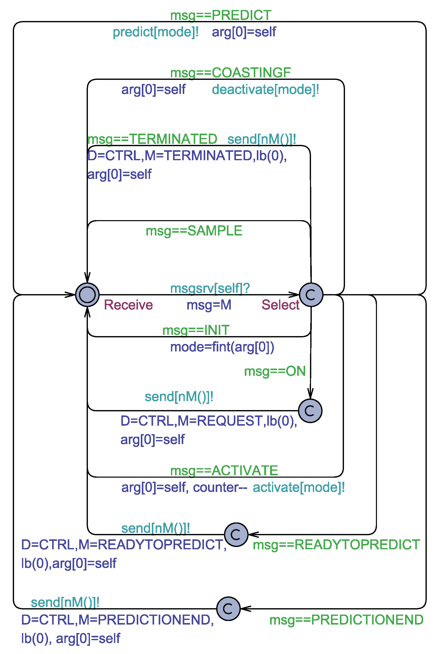
In order to reduce a Hybrid Theatre model onto Uppaal SMC, it is required to preliminarily define some information like the unique IDs for actors, delays, message names, message instances, and modes, together with suitable type ranges to control the creation of corresponding automata instances. Dynamism of message exchanges is ensured by anticipating a pool of message instances (see the avM[.] array in Figure 3). The send[.] channel gets a message instance ID through the nM() function, which returns the first available instance in the message pool. In the case the pool is under-dimensioned, an error arises during the operations of the model checker. When sending a message (see, e.g., Figure 4), the function lb(a) permits to establish the after value (lower bound), but sets the deadline to its infinite default value. Figure 3 shows the behaviour of each message instance (mi), which is an enhanced version of that used for basic Theatre [11]. One Lamport logical clock is associated to each theatre (PU). The local clock x permits the direct use of the after and deadline relative times. When after time units are elapsed in the scheduled location, the logical clock of this message is added to a priority queue associated with the PU of the destination actor. All the simultaneous messages enter the delivery location. From this location, provided the PU of the destination actor is free, after the smallest time Uppaal SMC can recognize, the message having the lowest logical clock is first delivered. Other details should be self-explanatory. It is worth noting that the bag of the just sent, but not yet delivered, messages is automatically formed by all the scheduled instances of Messages whose timing (including the logical clocks) ultimately reflects the control machine behaviour of the Theatre model. Non-determinism still exists for choosing between a message delivery and a simultaneously expiring delay. The HEMS model does not use delays, thus its behaviour is deterministic [36].
5. The Uppaal Model for the Home Energy Management System
The HEMS was firstly developed by using Actors and the Theatre architecture and subsequently reduced to Uppaal timed automata by exploiting the approach described in [11]. For this reason, in the following, the terms “Uppaal model” and “actor model” are interchangeable and express the same entity. The approach has been extended so as to take into account continuous modes. This section proposes the Uppaal models for the Controller, the EMeter, the EHVAC actor and those of all the other enhanced loads described in Section 3. Besides the EHVAC actor model, all the other load actors are modelled by using the same Uppaal template named Tabular Load template. This is because the consumption curves of all the appliances, except the HVAC, evolves as piece-wise constant functions (see Figure 2) and the Tabular Load is a configurable template whose behaviour evolves according to this kind of functions which are achieved through a tabular representation of distinct pairs . The Controller and the Meter, instead, do not make use of continuous modes. For simplicity, the template of the Load Manager is not shown since it only carries out the initialization phase of the system.
5.1. The Uppaal Model for the Tabular Load Actors
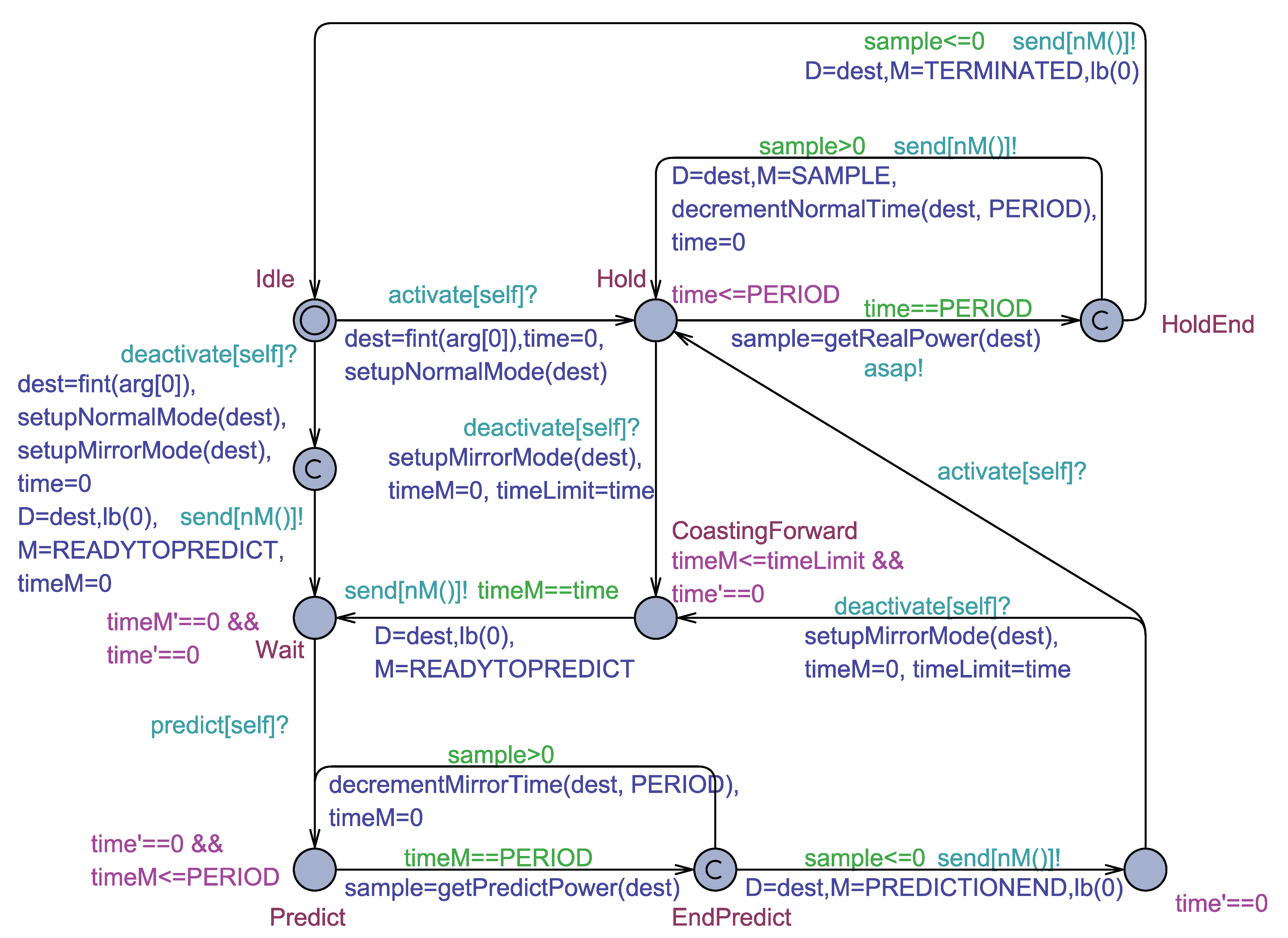
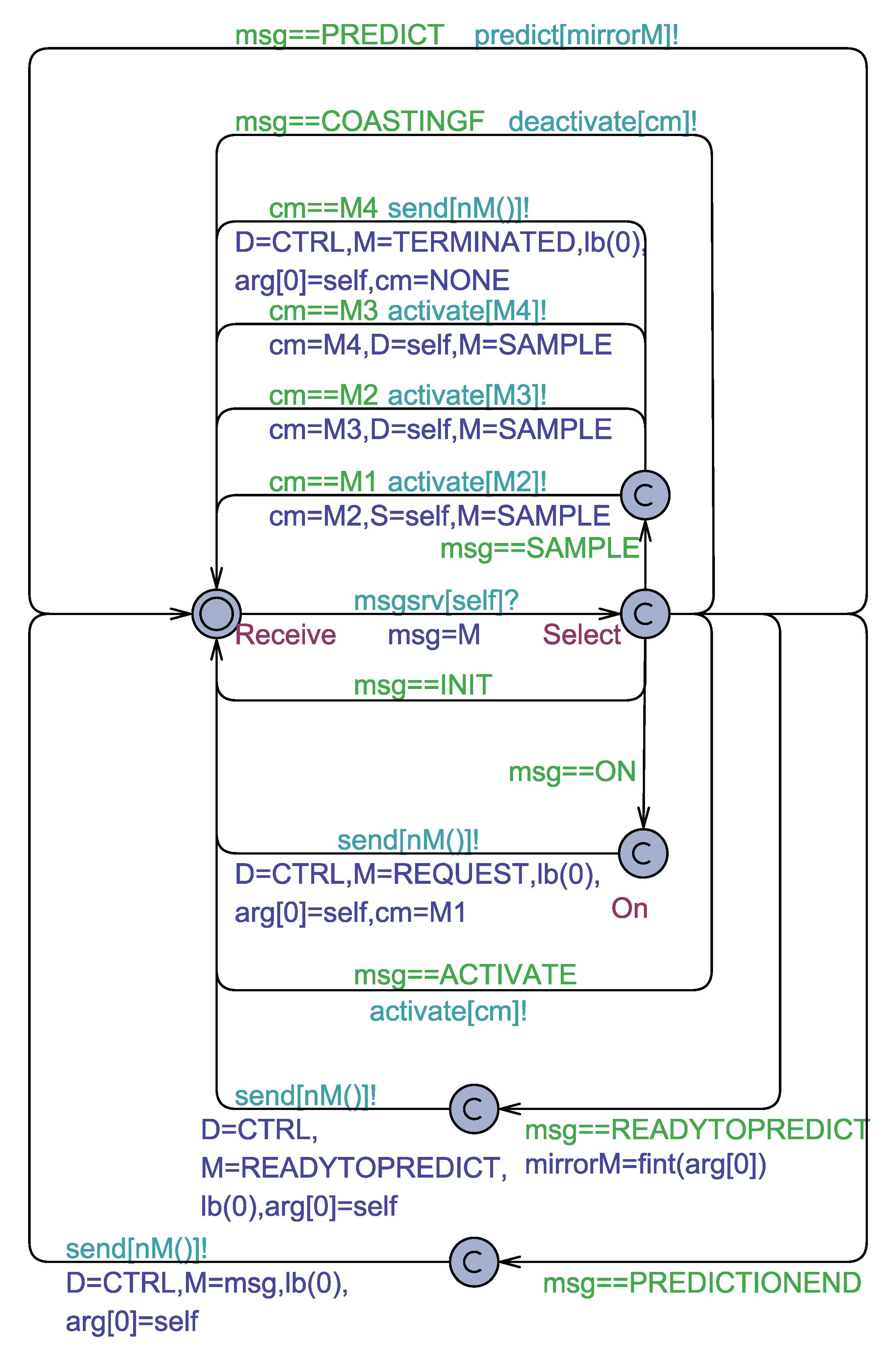
The model (see Figure 4) evolves according the three phases (i.e., coasting forward, prediction, active) described in Section 3. The communication between a tabular load and the controller relies on message exchange. The same holds for the communication originating from the mode of the tabular load and directed to the load itself. Communication from the load toward the mode is instead achieved by using the broadcast urgent channels deactivate[.], activate[.], and predict[.], which, respectively, are used to: deactivating and freezing out a mode (if active), and to start the coasting forward; resuming mode execution or making the mode active for the first time; starting the prediction phase. A load, after the INIT message, receives the ON message, thus starting the interactions with the controller by issuing a REQUEST for its admission. On receiving the COASTINGF message, the load deactivates its mode and stays at rest until the coasting forward completes and it receives a READYTOPREDICT coming from its mode. This message is then forwarded to the controller, which will reply with a PREDICT as soon as the prediction phase can start. At the end of the prediction phase, the mode sends a PREDICTIONEND to the load which, in turn, first sends this message to the controller and then waits for receiving an ACTIVATE. After being activated, the load receives a SAMPLE message each time the own mode completes the execution of the current constant piece of the power curve, i.e., the current pair. The TERMINATED message is received by the load when the mode completes its whole behaviour. This message is then sent to the controller to inform that the load is no longer active.
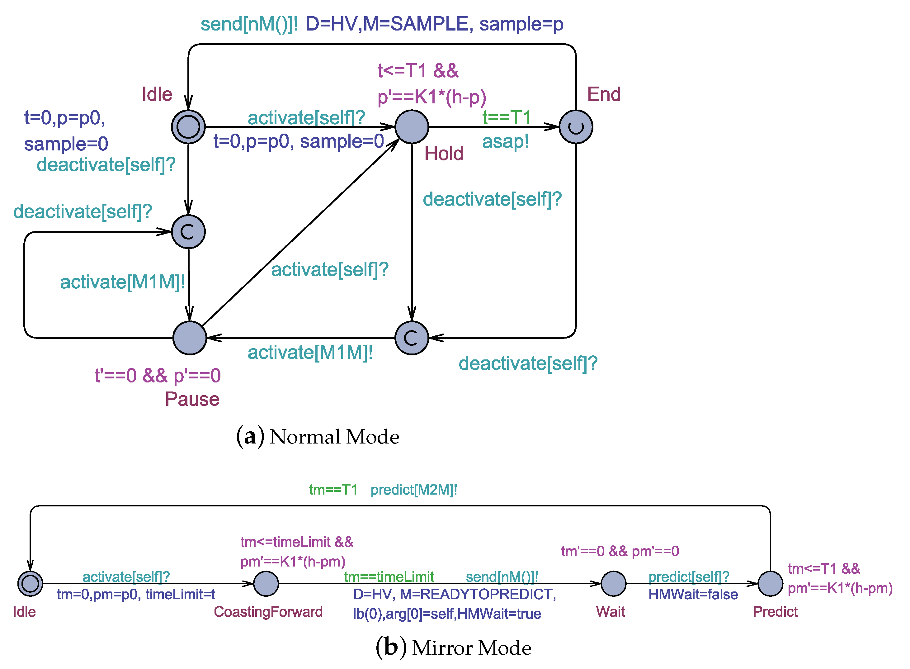
The mode of a tabular load is portrayed in Figure 5. It provides both the real and the predicted consumption curve of a load. In order to furnish the sampled values of these curves, the mode uses, respectively, the functions getRealPower(.) and getPredictedPower(.). The mode samples the consumption curve every PERIOD time units. Two clocks are exploited, namely time, for the real consumption curve, and timeM, for the predicted one. According to these clocks, the functions decrementNormalTime(.,.) and decrementMirrorTime(.,.) are used to go ahead, respectively, in the tables containing the tabular values of the real and the predicted power curves. The initial location of the automata is Idle, and the mode returns again in this location as it completes to provide the whole real consumption curve. A synchronization with the activate[.] broadcast urgent channel moves the automaton in the Hold location in which the real consumption curve of the load is sampled and provided. A synchronization with the deactivate[.] broadcast urgent channel leads the mode into the Wait location in which the two clocks are frozen (see the invariant ) and the mode becomes ready to start the prediction. The CoastingForward location is used for coasting forward, here timeM increases up to reach the value of the frozen time clock (see the invariant , where is set to the frozen value of time). A synchronization with the predict[.] broadcast urgent channel moves the mode into the Predict location in which the predicted consumption curve is sampled and provided. Here, only the clock time is frozen, whereas timeM grows up to reach the PERIOD value (see the invariant ). When the prediction completes, the mode moves back into the Hold location by following an activation, or into CoastingForward by following another deactivation.
5.2. The Uppaal Model for the HVAC actor
The following describes the actor model of the HVAC inverter heat pump considered as one appliance in the HEMS model. As emerges from Figure 2d, the power curve actually lasts about 110 time units, and it is given by the composition of four different continuous functions. As a consequence, four different modes, namely , , and , are required for generating, respectively, the four sub-curves. The mode and keep the power to a constant value, whereas and have, respectively, the following dynamic law and , where p is the power function, is its first derivative, and , and h are constants (i.e., , and ). The modes so far described are responsible for the behaviour of the actor when it is active. Further mirror modes, namely, respectively, , , and , are introduced to provide the actor behaviour during the coasting forward and the prediction phases.
Figure 6a shows the mode. Initially, the mode finds itself in the Idle location. By following instead a synchronization on the urgent broadcast channel activate[self], it moves to the Hold location in which the power function p varies according to the dynamic law of the normal mode and the clock t, which models the time of the mode, evolves too. Despite the current location, instead, by following a synchronization on the urgent broadcast channel deactivate[self] the mode reaches, without time passage, the Pause location in which the power function and the time are frozen (i.e., ). Just before reaching such a location, the mode activates its mirror counterpart through a synchronization on the urgent broadcast channel activate[M1M]. The mode stays in the location Hold as long as the invariant condition holds. Exiting from this location, the mode completes its behaviour reaching the End location and subsequently returns back to the Idle location sending a SAMPLE message to the HVAC actor. The other modes have a behaviour very close to that of and, for this reason, are not described.
The mode is shown in Figure 6b. The initial location of the mode is Idle. By following a synchronization on the urgent broadcast channel activate[self] it reaches the CoastingForward location. Here, the predicted power function starts to grow according to the same low of the power function of its corresponding normal mode . The coasting forward terminates as soon as the clock of the mirror mode reaches the same time reached by the normal mode . All of this is purposely expressed by the invariant . The variable is initialized on the arc outgoing the Idle location. On exiting the CoastingForward location, the mirror mode sends a READYTOPREDICT message to the HVAC actor and enters the Wait location. The mode remains here until it synchronizes with the urgent broadcast channel predict[self] and moves to the Predict location. Here, the predicted power evolves by following the same low of the real power of the mode . At the end of the prediction, the current mirror mode notifies the next mirror mode of the HVAC which, in this case, is the mode. It is worth noting that, once the prediction phase is started within a mirror mode, the next one has to continue this phase without executing the coasting forward. This is mirrored by the fact that exits from the Predict location by synchronizing with the broadcast urgent channel predict[M2M]. The other mirror modes have a behaviour similar to that of and, for this reason, are not reported. The only substantial difference is that the other mirror modes are required to hear a further synchronization when staying in the Idle location which permits them to start the mode behaviour by directly going into the Predict location, thus bypassing the coasting forward. The last mirror mode, i.e., the mode, on exiting the Predict location will send a message to the HVAC informing that the prediction phase is completed.
The model for the HVAC is reported in Figure 7. When active, the HVAC actor behaves as a finite state machine whose current state is defined by the current mode (cm). On receiving the ON message, the HVAC sets the first mode as its current mode, i.e., , and sends to the controller a request for activation. In the same way as for the tabular loads, by interacting with the controller, the HVAC moves first into the coasting forward phase, then into prediction and, finally, into the active phase. This last phase is triggered by receiving an ACTIVATE message. When the current mode terminates, i.e., a SAMPLE message is received, and then the next mode is activated. The behaviour of the appliance completes when the last mode, namely the one, terminates. As described in Section 3, the controller can stop the active phase and move again the HVAC into the coasting forward phase, each time a new load asks for its admission. Other details of the HVAC model should be self-explanatory.
5.3. The Uppaal Model for the Controller Actor
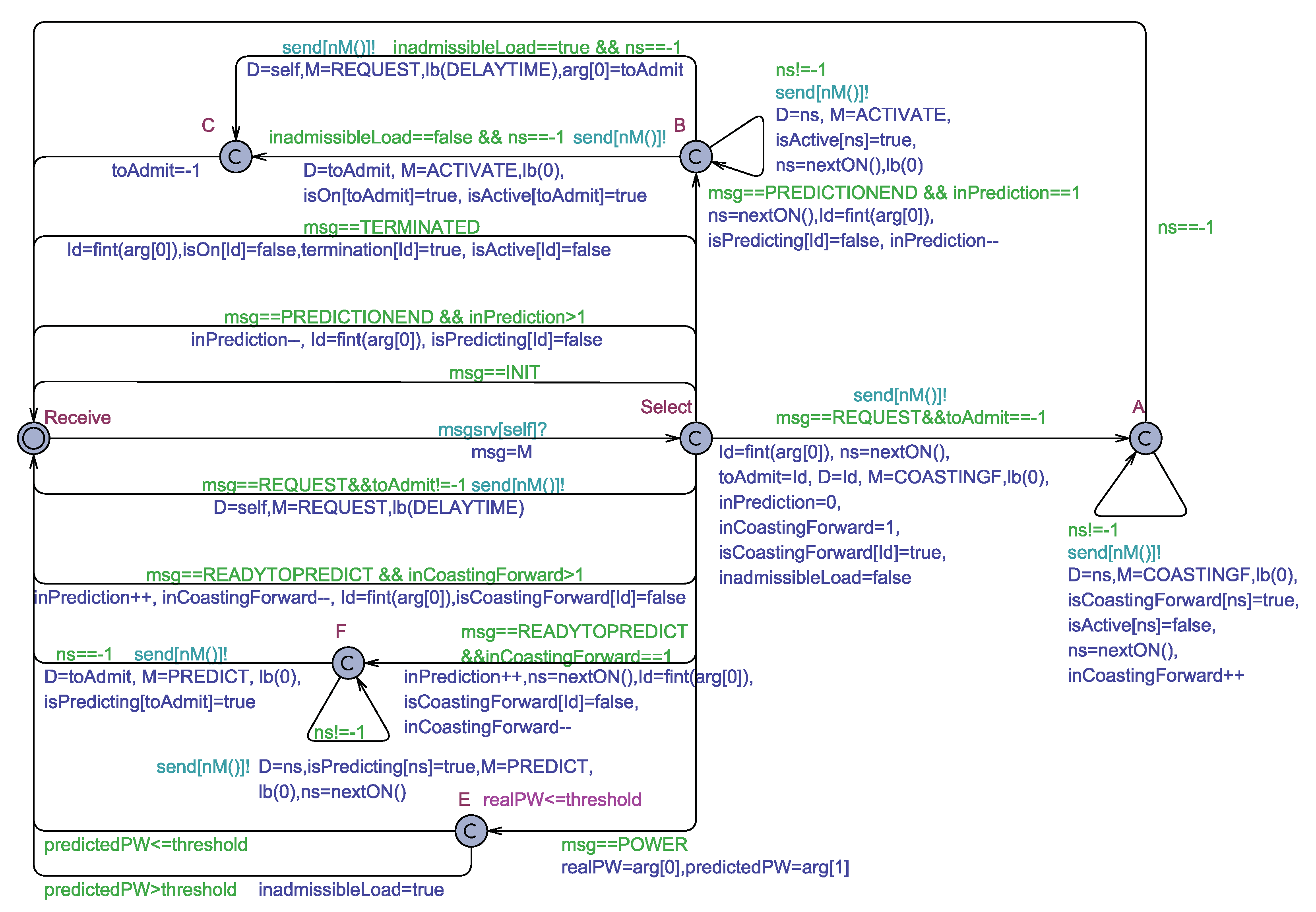
The Controller actor (see Figure 8) periodically receives POWER messages from the meter. One of such messages has two arguments carrying out information about the current power consumption, both real and predicted, of the whole system. Since all the loads stay simultaneously in the active or prediction phase (see Section 3), the two arguments cannot be at the same time greater than zero. The measured predicted power consumption will be greater than zero only if a new load sends a REQUEST and the HEMS switches in prediction. During prediction, in the case the predicted power is found to be greater than the consumption threshold, the variable inadmissibleLoad is set to true, indicating that the new load cannot be served at this moment. In such a case, the current request is deferred by DELAYTIME time units. In no case, the real power consumption of the system can exceed the threshold. In order to check this condition, the invariant is set for the location E of the controller automaton. On receiving a REQUEST message, the controller evolves according to the schema described in the following:
- the controller sends to each active load (if any) the COASTINGF message;
- as soon as all the loads replied with a READYTOPREDICT, the controller sends them a PREDICT message;
- when all the loads replied with a PREDICTIONEND, the controller checks the value of the inadmissibleLoad variable, thus deciding to admit or defer the new load. In the former case, an ACTIVATE message is sent to the new load;
- an ACTIVATE message is sent to each previously active loads.
In the case multiple REQUESTs arrive to the controller, only the first one is considered, while the others are deferred by DELAYTIME time units. Besides the entities so far described, the controller operates by using the variables and the functions reported in Table 2. Each array in the table has a length equal to the number of loads existing in the system. Other details of the controller should be self-explanatory.
5.4. The Uppaal Model for the Meter Actor
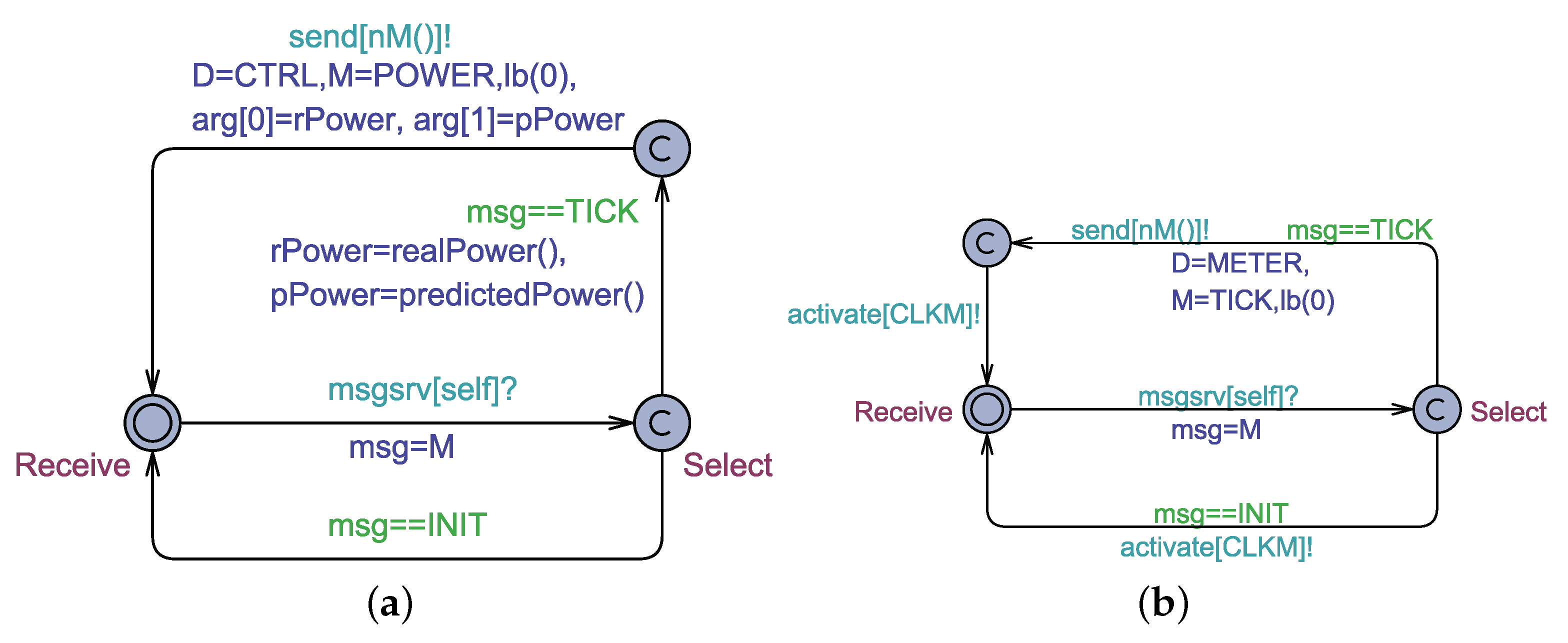
The meter (see Figure 9a) has a periodic behaviour, which in turn depends on the Clock actor (see Figure 9b), which sends a TICK message to the meter after each PERIOD time unit. The meter reacts to a TICK by sending a POWER message to the controller together with the current value of the total load power consumption, both real and predicted, obtained by invoking, respectively, the realPower() and the predictedPower() function. In such a way, the sampling frequency of the HEMS is defined by the PERIOD value. Changing only this value, thought, is not enough to evaluate how the point-of-view of the controller changes with respect to the actual value of the real and predicted power consumption curves. In order to achieve this, it is required that the meter samples the consumption curves with a given sample but only a subset of these samples are then sent to the meter. A SCALE integer factor is introduced, and the behaviour of the meter automaton is slightly modified so as to sent the power messages to the controller every SCALE times. As a consequence, the sampling time of the controller is given by , but the sampling time with which the power curves are sampled by the meter remains to be .
6. Property Checking and Experimental Results
The goal of the analysis phase is two-fold. First, it is devoted to checking if the controller is able to properly behave, i.e., if the prediction policy is able to prevent the overcoming of the threshold during system operation. Second, it is devoted to checking the proper coupling between the cyber and the physical part of the system, i.e., to check if the cyber part of the HEMS is able to correctly interact with the physical part given a specific value of the sampling frequency. As described in Section 5.4, the sampling period of the meter is determined by PERIOD, whereas the period with which the controller receives information about the consumption curves is given by SCALE×PERIOD. In what follows, PERIOD is set to . This value was chosen experimentally by checking that a smaller value for the period did not affect the resolution of the observed consumption curves.
The behaviour of the HEMS reduced to Uppaal SMC was checked in two cases: (a) the control strategy is not required, i.e., a threshold value is set which permits the contemporary admission of all the loads in the system at the same time; and (b) the control policy is required to prevent the overcome of the threshold. While executing the experiments, in no case, the invariant (see Section 5.3) of the controller was violated. All the experiments refer to the critical case in which all the loads immediately ask for their admission to the controller.
A first set of Metric Interval Temporal Logic (MITL) queries [18] were issued with a threshold set to 7, a SCALE set to 1, and a DELAYTIME set to 1. For each result, where applicable, are reported the number of runs requested by the Uppaal SMC to get the result and the confidence interval of the result with a confidence level of .
Q1: Pr[<=2000](<>predictedPower()>threshold)
Q2: Pr[<=2000](<>realPower()>threshold)
R1–R2: (29 runs) Pr(<> ...) in [0,0.0981446] with confidence 0.95.
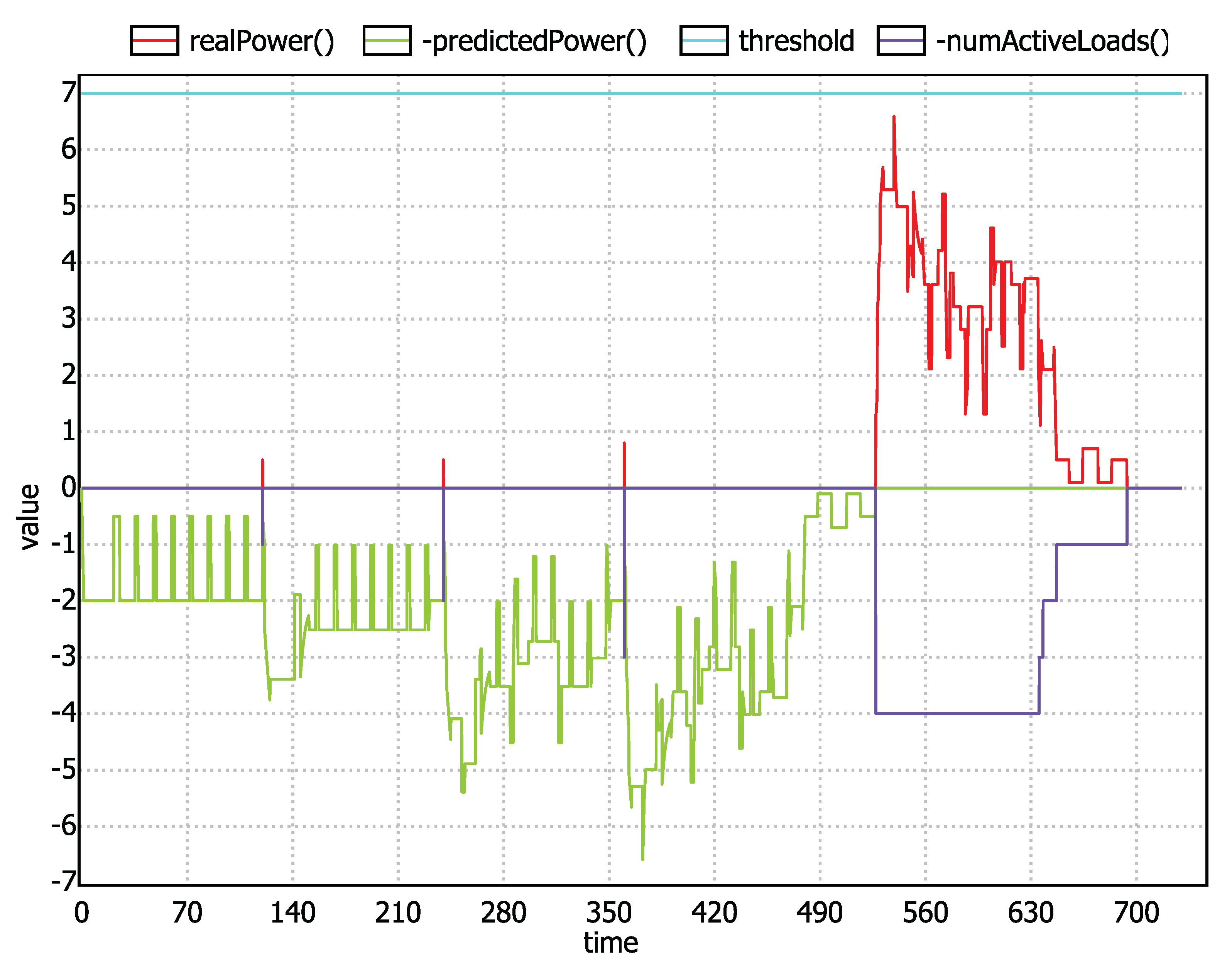
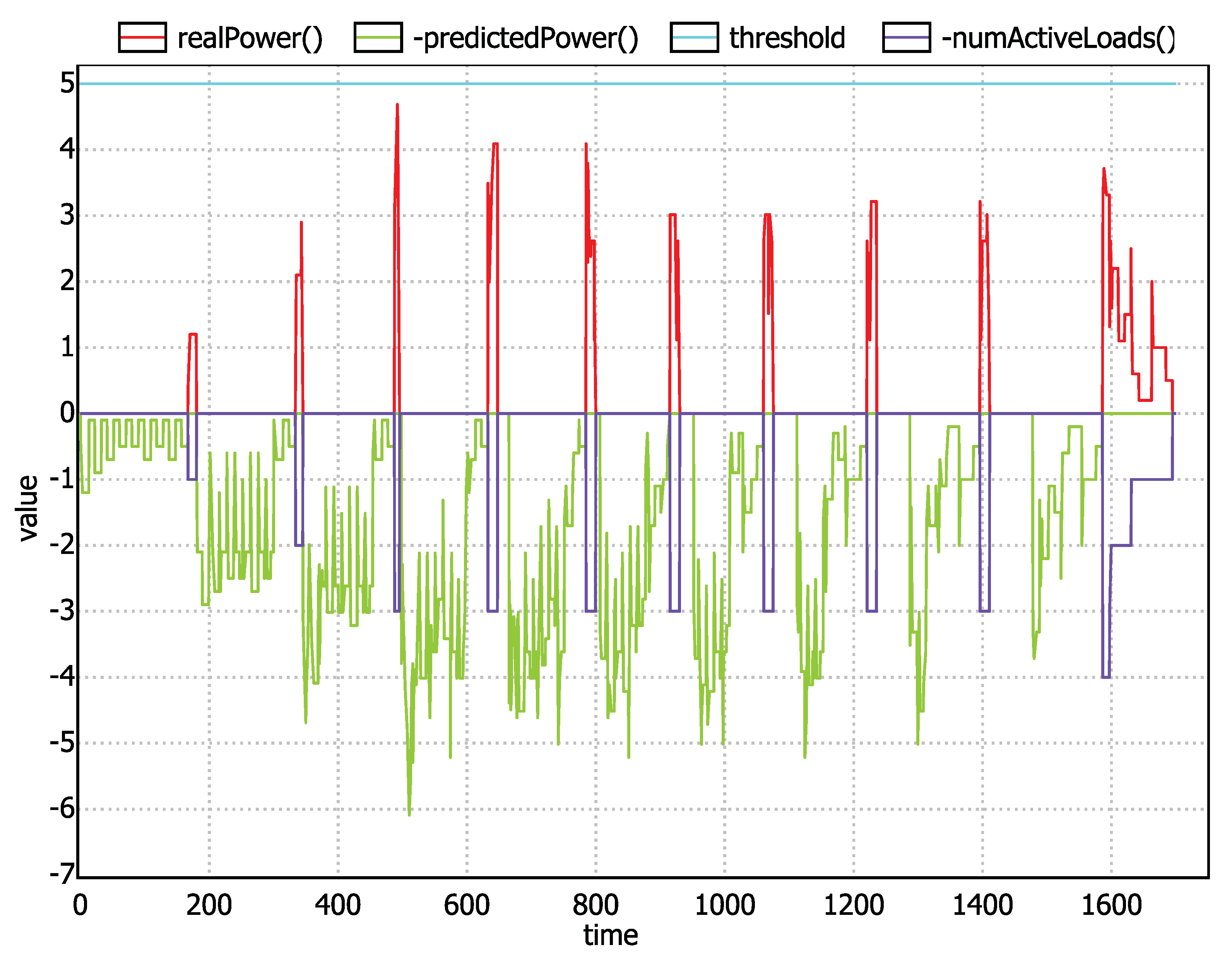
Q3: simulate [<=700] { realPower(), -predictedPower(), threshold, -numActiveLoads() }
R3: The picture in Figure 10.
Q4: Pr[<=700]([] (Hvac(HV).msgCounter==1 && Hvac(HV).msg==ON) ||
(Hvac(HV).msgCounter!=1) )
Q5: Pr[<=700]([] (Hvac(HV).msgCounter==2 && Hvac(HV).msg==COASTINGF) ||
(Hvac(HV).msgCounter!=2) )
Q6: Pr[<=700]([] (Hvac(HV).msgCounter==3 && Hvac(HV).msg==READYTOPREDICT)||
(Hvac(HV).msgCounter!=3) )
Q7: Pr[<=700]([] (Hvac(HV).msgCounter==4 && Hvac(HV).msg==PREDICT)||
(Hvac(HV).msgCounter!=4) )
Q8: Pr[<=700]([] (Hvac(HV).msgCounter==5 && Hvac(HV).msg==PREDICTIONEND)||
(Hvac(HV).msgCounter!=5) )
Q9: Pr[<=700]([] (Hvac(HV).msgCounter==6 && Hvac(HV).msg==ACTIVATE)||
(Hvac(HV).msgCounter!=6) )
R4–R9: (29 runs) Pr([] ...) in [0.901855,1] with confidence 0.95.
Figure 10.
The real and predicted power consumption (in KW) and the number of active loads during load scheduling with a threshold of 7 (KW).
Figure 10.
The real and predicted power consumption (in KW) and the number of active loads during load scheduling with a threshold of 7 (KW).

Queries and are devoted to check, within a time interval of 2000 time units, the probability to find, respectively, the predicted power and the real power greater than the threshold. The results and indicate that these events are practically impossible as they have as confidence interval.
The query asks the Uppaal SMC verifier to simulate, in a time interval of 700 time units, the evolution of: the real power consumption, the predicted power, and the number of active loads. From the simulation outcomes, it is possible to see how the HEMS evolves and how the controller evaluates the cumulative predicted power consumption curve as soon as new loads ask for their admission. When the controller has considered the cumulative prediction curves of all the loads, all the loads are switched into active.
The queries from to checks if the HVAC receives the control messages in the right order. By considering the query results from to , it is possible to state that the HEMS behaves properly.
A further set of queries were issued to check the correctness of the HEMS in the case the controller has to defer the admission of some loads in order to meet the threshold. In this second scenario, a threshold set to 5 and the DELAYTIME set to 15 were considered. SCALE and PERIOD have remained unchanged.
Q10: Pr[<=1700](<>realPower()>threshold)
R10: (29 runs) Pr(<> ...) in [0,0.0981446] with confidence 0.95.
Q11: Pr[<=1700](<>predictedPower()>threshold)
R11: (29 runs) Pr(<> ...) in [0.901855,1] with confidence 0.95.
Q12: Pr[<=2000]([] now < 1999 || forall(i : int[0,TABLOADS+ODELOADS-1]) termination[i]==true
R12: (29 runs) Pr([] ...) in [0.901855,1] with confidence 0.95.
Q13: simulate [<=1700] { realPower(), -predictedPower(), threshold, -numActiveLoads() }
R13: The picture in Figure 11.
The query checks the probability of finding the real power greater than the threshold. Furthermore, in this case, states that this event is practically impossible. The query instead checks the probability to have the predicted power consumption greater than the threshold. In such a case, instead, the probability of this event is very high, and it can be considered as practically certain. The query checks the probability to have all the loads terminated at the 2000th time instant. confirms that such an event is practically certain. By considering , and , it is possible to conclude that the exploited admission control policy is really effective in managing the activation scheduling of the loads. Query is devoted to showing a simulation tied to the evolution of the HEMS in terms of real power, predicted power and number of active loads.
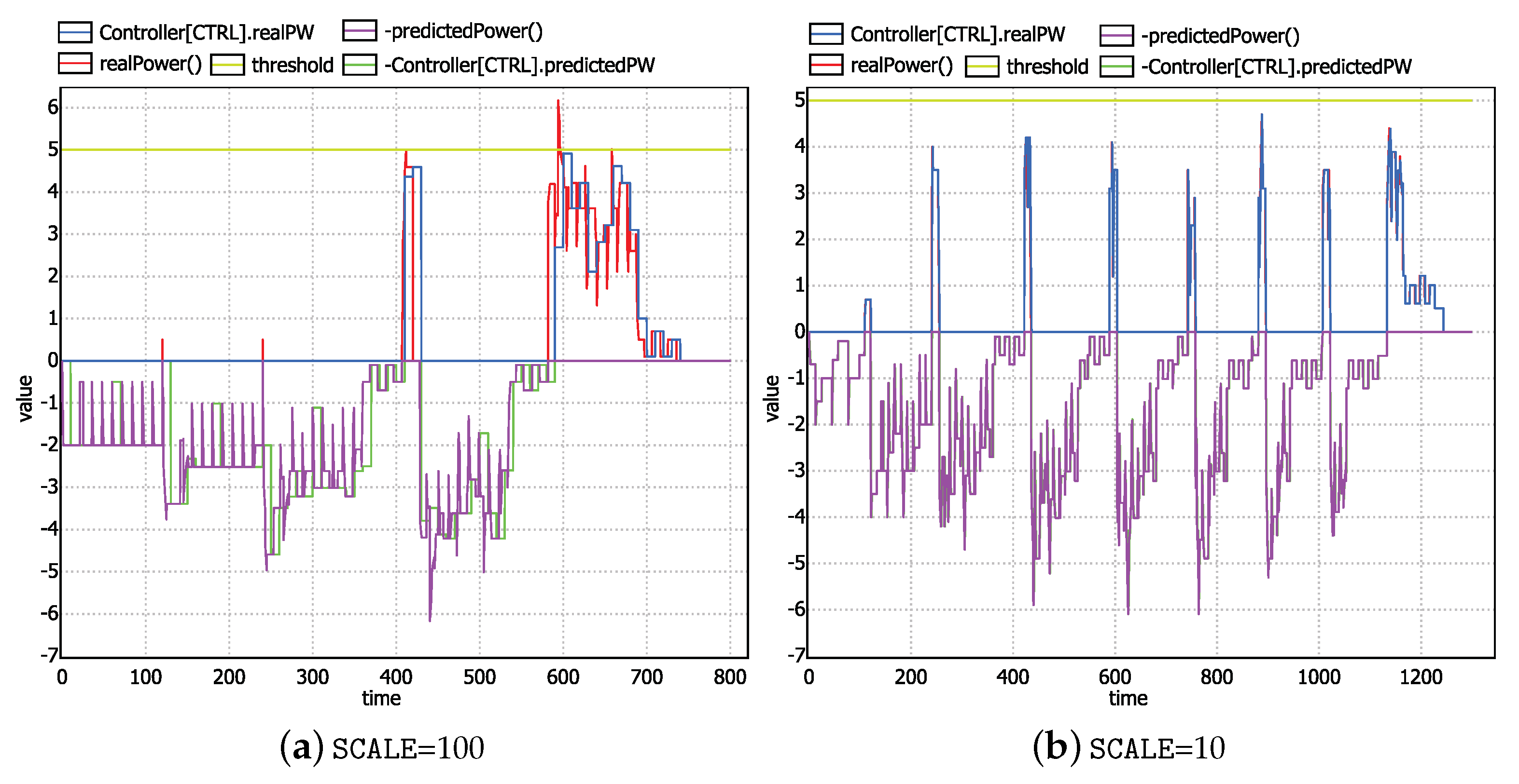
In order to assess how a change in the sampling frequency of the controller affects its ability to control the load scheduling, two other scenarios were considered by varying the value of the SCALE variable. More in detail, by setting SCALE to 100, from Figure 12a it follows that the controller is not able to correctly schedule the loads. In fact, the real power consumption overcame the threshold during load activation. This is also witnessed by , where it emerges that the probability to have the real power over the threshold has a confidence interval of . A more subtle case is that concerning the SCALE set to 10. In this case, a single simulation is not able to highlight any point in which the real power overcomes the threshold (see Figure 12b). A deeper analysis carried out by using the statistical model checker shows instead that, by considering 364 runs, the probability to have a threshold violation has a confidence interval of . In other words, with a SCALE set to 10, the controller is not able to properly behave.
Q14:
R14: (79 runs) Pr(<> ...) in [0.893009,0.992099] with confidence 0.95.
Q15:
R15: (364 runs) Pr(<> ...) in [0.29207,0.391866] with confidence 0.95.
7. Conclusions
This paper proposed an approach exploitable for developing Home Energy Management Systems (HEMSs). The approach leverages hybrid actors [12], the Theatre infrastructure [11], and model continuity [16]. The assessment of the system properties was achieved by preliminarily reducing the Theatre model onto the Uppaal hybrid timed automata and subsequently by using the statistical model checker.
The considered HEMS case study was chosen for highlighting the effectiveness and usability of the approach. The goal of the case study was two-folds: (i) evaluating how the setting of a given sampling frequency affects the behaviour of the whole HEMS; (ii) experimenting with an admission control policy able to prevent an overload upfront by predicting the effect that the admission of a new load will have on the consumption curve of the whole system. Ongoing and future work is geared at:
- Extending the case study by considering more complex scheduling policies and by using a more general deterministic version of Theatre actors;
- Completing the development of the proposed HEMS with preliminary and final system implementation;
- Enhancing the capabilities of the envGateway by offering basic design constructs and mechanisms for simplifying modelling and analysis of more complex physical environments;
- Experimenting with the proposed approach in more-general IoT-based applications, e.g., in augmented environments like smart homes and smart offices;
- Investigating the possibility of exhaustive model checking a Hybrid Theatre model, by following an approach similar to that adopted in Hybrid Rebeca [12].
Author Contributions
Formal analysis, F.C. and L.N.; Methodology, F.C. and L.N.; Software, F.C. and L.N.; Writing—Review and Editing: F.C. and L.N. The contribution of the authors is equal. All authors have read and agreed to the published version of the manuscript.
Funding
This research received no external funding.
Institutional Review Board Statement
Not applicable.
Informed Consent Statement
Not applicable.
Data Availability Statement
Not applicable.
Conflicts of Interest
The authors declare no conflict of interest.
References
- Saleem, Y.; Crespi, N.; Rehmani, M.H.; Copeland, R. Internet of Things-aided Smart Grid: Technologies, Architectures, Applications, Prototypes, and Future Research Directions. IEEE Access 2019. [Google Scholar] [CrossRef]
- Pawlaszczyk, D.; Strassburger, S. Scalability in Distributed Simulations of Agent-Based Models. In Proceedings of the Winter Simulation Conference (WSC), Austin, TX, USA, 13–16 December 2009; pp. 1189–1200. [Google Scholar]
- Siebert, L.C.; Ferreira, L.R.; Yamakawa, E.K.; Custódio, E.S.; Aoki, A.R.; Fernandes, T.S.P.; Cardoso, K.H. Centralized and decentralized approaches to demand response using smart plugs. In Proceedings of the 2014 IEEE PES T D Conference and Exposition, Chicago, IL, USA, 14–17 April 2014; pp. 1–5. [Google Scholar] [CrossRef]
- Errapotu, S.M.; Wang, J.; Gong, Y.; Cho, J.; Pan, M.; Han, Z. SAFE: Secure Appliance Scheduling for Flexible and Efficient Energy Consumption for Smart Home IoT. IEEE Internet Things J. 2018, 5, 4380–4391. [Google Scholar] [CrossRef]
- Moulema, P.; Mallapuram, S.; Yu, W.; Griffith, D.; Golmie, N.; Su, D. Admission Control-Based Load Protection in the Smart Grid. In Security and Privacy in Cyber Physical Systems; John Wiley & Sons, Ltd.: Hoboken, NY, USA, 2017; Chapter 19; pp. 399–421. [Google Scholar] [CrossRef]
- Jaradat, M.; Jarrah, M.; Jararweh, Y.; Al-Ayyoub, M.; Bousselham, A. Integration of renewable energy in demand-side management for home appliances. In Proceedings of the 2014 International Renewable and Sustainable Energy Conference (IRSEC), Ouarzazate, Morocco, 17–19 October 2014; pp. 571–576. [Google Scholar] [CrossRef]
- Chaouch, H.; Ben Hadj Slama, J. Modeling and simulation of appliances scheduling in the smart home for managing energy. In Proceedings of the 2014 International Conference on Electrical Sciences and Technologies in Maghreb (CISTEM), Tunis, Tunisia, 3–6 November 2014; pp. 1–5. [Google Scholar] [CrossRef]
- Mocanu, E.; Mocanu, D.C.; Nguyen, P.H.; Liotta, A.; Webber, M.E.; Gibescu, M.; Slootweg, J.G. On-line Building Energy Optimization using Deep Reinforcement Learning. IEEE Trans. Smart Grid 2018, 10, 3698–3708. [Google Scholar] [CrossRef] [Green Version]
- Tundis, A.; Faizan, A.; Mühlhäuser, M. A Feature-Based Model for the Identification of Electrical Devices in Smart Environments. Sensors 2019, 19, 2611. [Google Scholar] [CrossRef] [PubMed] [Green Version]
- Kim, K.D.; Kumar, P. An Overview and Some Challenges in Cyber-Physical Systems. J. Indian Inst. Sci. 2013, 93, 341–352. [Google Scholar]
- Nigro, L.; Sciammarella, P.F. Qualitative and Quantitative Model Checking of Distributed Probabilistic Timed Actors. Simul. Model. Pract. Theory 2018, 87, 343–368. [Google Scholar] [CrossRef]
- Jahandideh, I.; Ghassemi, F.; Sirjani, M. Hybrid Rebeca: Modeling and Analyzing of Cyber-Physical Systems. In Cyber Physical Systems. Model-Based Design; Springer: Cham, Switzerland, 2019. [Google Scholar]
- Lee, E.A. The Problem with Threads. Computer 2006, 39, 33–42. [Google Scholar] [CrossRef]
- Nigro, C.; Nigro, L.; Sciammarella, P.F. Modelling and analysis of multi-agent systems using UPPAAL SMC. Int. J. Simul. Process. Model. 2018, 13, 73. [Google Scholar] [CrossRef]
- Cicirelli, F.; Nigro, L. Control Centric Framework for Model Continuity in Time-dependent Multi-agent Systems. Concurr. Comput. Pract. Exper. 2016, 28, 3333–3356. [Google Scholar] [CrossRef]
- Cicirelli, F.; Nigro, L.; Sciammarella, P.F. Model continuity in cyber-physical systems: A control-centered methodology based on agents. Simul. Model. Pract. Theory 2018, 83, 93–107. [Google Scholar] [CrossRef]
- Agha, G.; Palmskog, K. A Survey of Statistical Model Checking. ACM Trans. Model. Comput. Simul. 2018, 28, 6:1–6:39. [Google Scholar] [CrossRef]
- David, A.; Larsen, K.G.; Legay, A.; Mikuăionis, M.; Poulsen, D.B. Uppaal SMC Tutorial. Int. J. Softw. Tools Technol. Transf. 2015, 17, 397–415. [Google Scholar] [CrossRef] [Green Version]
- Cicirelli, F.; Nigro, L. Home Energy Management Using Theatre with Hybrid Actors. In Proceedings of the 23rd IEEE/ACM International Symposium on Distributed Simulation and Real Time Applications, Cosenza, Italy, 7–9 October 2019; pp. 162–169. [Google Scholar]
- Cicirelli, F.; Nigro, L. Using Deterministic Theatre for Energy Management in Smart Environments. In Sustainable Intelligent Systems; Joshi, A., Nagar, A.K., Marín-Raventós, G., Eds.; Springer: Singapore, 2021; pp. 189–214. [Google Scholar] [CrossRef]
- Agha, G. Actors: A Model of Concurrent Computation in Distributed Systems; MIT Press: Cambridge, MA, USA, 1986. [Google Scholar]
- Lohstroh, M.; Lee, E.A. Deterministic Actors. In Proceedings of the 2019 Forum for Specification and Design Languages (FDL), Southampton, UK, 2–4 September 2019; pp. 1–8. [Google Scholar] [CrossRef]
- Sirjani, M.; Lee, E.A.; Khamespanah, E. Verification of Cyberphysical Systems. Mathematics 2020, 8, 1068. [Google Scholar] [CrossRef]
- Jafari, A.; Khamespanah, E.; Sirjani, M.; Hermanns, H.; Cimini, M. PTRebeca: Modeling and analysis of distributed and asynchronous systems. Sci. Comput. Program. 2016, 128, 22–50. [Google Scholar] [CrossRef]
- Cicirelli, F.; Nigro, L.; Sciammarella, P.F. Seamless Development in Java of Distributed Real-Time Systems using Actors. Int. J. Simul. Process. Model. 2020, 15, 13. [Google Scholar] [CrossRef]
- Remani, T.; Jasmin, E.A.; Ahamed, T.P.I. Residential Load Scheduling With Renewable Generation in the Smart Grid: A Reinforcement Learning Approach. IEEE Syst. J. 2019, 13, 3283–3294. [Google Scholar] [CrossRef]
- O’Neill, D.; Levorato, M.; Goldsmith, A.; Mitra, U. Residential Demand Response Using Reinforcement Learning. In Proceedings of the 2010 First IEEE International Conference on Smart Grid Communications, Gaithersburg, MD, USA, 4–6 October 2010; pp. 409–414. [Google Scholar] [CrossRef]
- Palensky, P.; Dietrich, D. Demand Side Management: Demand Response, Intelligent Energy Systems, and Smart Loads. IEEE Trans. Ind. Inform. 2011, 7, 381–388. [Google Scholar] [CrossRef] [Green Version]
- Cicirelli, F.; Grimaldi, D.; Furfaro, A.; Nigro, L.; Pupo, F. MADAMS: A Software Architecture for the Management of Networked Measurement Services. Comput. Stand. Interfaces 2006, 28, 396–411. [Google Scholar] [CrossRef]
- Nigro, L.; Sciammarella, P.F. Time Synchronization in Wireless Sensor Networks: A Modeling and Analysis Experience Using Theatre. In Proceedings of the 2018 IEEE/ACM 22nd International Symposium on Distributed Simulation and Real Time Applications (DS-RT), Madrid, Spain, 15–17 October 2018; pp. 1–8. [Google Scholar] [CrossRef]
- Karmani, R.K.; Agha, G. Actors. In Encyclopedia of Parallel Computing; Padua, D., Ed.; Springer: Boston, MA, USA, 2011; pp. 1–11. [Google Scholar] [CrossRef]
- Sirjani, M. Power is Overrated, Go for Friendliness! Expressiveness, Faithfulness, and Usability in Modeling: The Actor Experience. In Principles of Modeling: Essays Dedicated to Edward A. Lee on the Occasion of His 60th Birthday; Lohstroh, M., Derler, P., Sirjani, M., Eds.; Springer International Publishing: Cham, Switzerland, 2018; pp. 423–448. [Google Scholar] [CrossRef]
- Henzinger, T.A. The Theory of Hybrid Automata. In Verification of Digital and Hybrid Systems; Inan, M.K., Kurshan, R.P., Eds.; Springer: Berlin/Heidelberg, Germany, 2000; pp. 265–292. [Google Scholar] [CrossRef]
- Lohstroh, M.; Lee, E. An Interface Theory for the Internet of Things. Softw. Eng. Form. Methods 2015, 9276, 20–34. [Google Scholar] [CrossRef] [Green Version]
- Lamport, L. Time, clocks and the ordering of events in a distributed system. Commun. ACM 1978, 21, 558–565. [Google Scholar] [CrossRef]
- Jerad, C.; Lee, E.A. Deterministic Timing for the Industrial Internet of Things. In Proceedings of the 2018 IEEE International Conference on Industrial Internet (ICII), Seattle, WA, USA, 21–23 October 2018; pp. 13–22. [Google Scholar] [CrossRef]
Figure 1.
The architecture of the considered HEMS.

Figure 2.
(a–d) The consumption curve (in KW) of the considered appliances vs. time.

Figure 3.
The Message automaton.

Figure 4.
The Tabular Load actor model.

Figure 5.
The Mode for the Load actor model.

Figure 6.
A normal mode and a mirror mode of the HVAC actor.

Figure 7.
The HVAC actor model.

Figure 8.
The Uppaal model of the controller.

Figure 9.
The Meter (a) and the Clock (b) actor.

Figure 11.
The real power and predicted power consumption (in KW) and number of active loads during load scheduling with a threshold of 5 (KW).
Figure 11.
The real power and predicted power consumption (in KW) and number of active loads during load scheduling with a threshold of 5 (KW).

Figure 12.
The consumption curve (in KW) of the considered appliances vs. time in the case two different SCALE factors are used.
Figure 12.
The consumption curve (in KW) of the considered appliances vs. time in the case two different SCALE factors are used.


Table 1.
Messages managed by the actors’ templates of Uppaal.
| Message Type | Sender | Receiver | Description |
|---|---|---|---|
| INIT | Load Manager | ELoad | Setting-up load parameters |
| ON | Load Manager | ELoad | Switch-on a load. After switched-on, the load sends a REQUEST message to the controller |
| REQUEST | ELoad | Controller | Used by a load to ask the controller to become active |
| ACTIVATE | Controller | ELoad | Activates and makes operating a load. A previously active load resumes its operation from the point it was suspended last. An active load consumes real power |
| COASTINGF | Controller | ELoad | Suspends load activity (if any) and prepares the load to predict its remaining power consumption |
| READYTOPREDICT | ELoad | Controller | Communicates to the controller that the coasting forward phase is completed and that the load is ready to simulate its remaining power consumption |
| Load Mode | ELoad | Used to communicate that the current mode completed the coasting forward | |
| PREDICT | Controller | ELoad | Communicates that a load can start the prediction phase |
| PREDICTIONEND | Load Mode | ELoad | Used to communicate that the current mode completed its simulation phase |
| ELoad | Controller | Used to communicate that a load completed its simulation phase | |
| TERMINATED | ELoad | Controlled | Used to communicate that a load completed its task |
| SAMPLE | Load Mode | ELoad | Used to communicate that the current mode completed its behaviour |
| POWER | Meter | Controller | Communicates the instantaneous cumulative power consumption, both predicted and real, of the loads |
Table 2.
Variables and functions exploited by the Controller actor.
| Identifier | Type | Description |
|---|---|---|
| isOn | boolean array | an element is true if the corresponding load was admitted by the controller |
| nextON | function | iterates on the array of admitted loads |
| inPrediction | integer var | number of loads which are in prediction |
| inCoastingForward | integer var | number of loads which are in coasting forward |
| isCoastingForward | boolean array | an element is true if the corresponding load is in coasting forward |
| toAdmit | integer var | the load that asked for admission |
| isActive | boolean array | an element is true if the corresponding load is active |
| termination | boolean array | indicates whether a load has completed its execution |
Publisher’s Note: MDPI stays neutral with regard to jurisdictional claims in published maps and institutional affiliations. |
© 2021 by the authors. Licensee MDPI, Basel, Switzerland. This article is an open access article distributed under the terms and conditions of the Creative Commons Attribution (CC BY) license (https://creativecommons.org/licenses/by/4.0/).
Share and Cite
MDPI and ACS Style
Cicirelli, F.; Nigro, L. Admission Control in Home Energy Management Systems Using Theatre and Hybrid Actors. Modelling 2021, 2, 288-307. https://0-doi-org.brum.beds.ac.uk/10.3390/modelling2020015
AMA Style
Cicirelli F, Nigro L. Admission Control in Home Energy Management Systems Using Theatre and Hybrid Actors. Modelling. 2021; 2(2):288-307. https://0-doi-org.brum.beds.ac.uk/10.3390/modelling2020015
Chicago/Turabian StyleCicirelli, Franco, and Libero Nigro. 2021. "Admission Control in Home Energy Management Systems Using Theatre and Hybrid Actors" Modelling 2, no. 2: 288-307. https://0-doi-org.brum.beds.ac.uk/10.3390/modelling2020015