Remarks on the Boundary Conditions for a Serre-Type Model Extended to Intermediate-Waters

Abstract

Numerical models are useful tools for studying complex wave–wave and wave–current interactions in coastal areas. They are also very useful for assessing the potential risks of flooding, hydrodynamic actions on coastal protection structures, bathymetric changes along the coast, and scour phenomena on structures’ foundations. In the coastal zone, there are shallow-water conditions where several nonlinear processes occur. These processes change the flow patterns and interact with the moving bottom. Only fully nonlinear models with the addition of dispersive terms have the potential to reproduce all phenomena with sufficient accuracy. The Boussinesq and Serre models have such characteristics. However, both standard versions of these models are weakly dispersive, being restricted to shallow-water conditions. The need to extend them to deeper waters has given rise to several works that, essentially, add more or fewer terms of dispersive origin. This approach is followed here, giving rise to a set of extended Serre equations up to kh ≈ π. Based on the wavemaker theory, it is also shown that for kh > π/10, the input boundary condition obtained for shallow-waters within the Airy wave theory for 2D waves is not valid. A better estimate for the input wave that satisfies a desired value of kh can be obtained considering a geometrical modification of the conventional shape of the classic piston wavemaker by a limited depth $\theta h$, with $\theta \le$ 1.0.

1. Introduction

Typically, the structures commonly found in the coastal environment, such as groynes and breakwaters, are implanted in intermediate- and shallow-waters. The design of such structures requires knowledge of the flow characteristics associated with currents and surface waves. Knowing the flow characteristics is also essential to predict changes in the bottom, as they lead to the accretion and erosion of sediments that are often harmful, especially around coastal protections.

By the end of the 1970s, due to the limited knowledge that existed at the time and the low capacity of computational tools, linear wave theory was often used to simulate the processes of the refraction and diffraction of waves. In the 1980s, more advanced models for the purpose of simulating both refraction and diffraction phenomena were commonly used. Examples of such models are those of Berkhoff et al. [1], Kirby and Dalrymple [2], Booij [3], Kirby [4], and Dalrymple [5]. However, such models are based on linear theory, so they should not be used in shallow-water conditions.

As noted in [6], at that time, the numerical simulation of coastal processes was carried out using models that solved Saint-Venant-type equations [7]. However, such models are unable to simulate phenomena of dispersive origin, which are typical of shallow-waters and for certain types of waves. Indeed, as shown in [8], Saint-Venant type models, due to their mathematical and conceptual limitations, are unable to produce satisfactory numerical results during long periods of analysis. In addition to the common processes of refraction and diffraction, the phenomena of the swelling, reflection, and breaking of waves are also typical of shallow-waters. Such phenomena overlap, so it is the combined action of all of them that produces the flow patterns typical of coastal areas.

Additionally, according to [6], a variety of factors allow the development and use of less limited and more robust mathematical models. In the last three decades, the use of better equipment, more efficient experimental methods, and a deeper theoretical knowledge of physical phenomena have been decisive for the increasing refinement of numerical methods. Major developments in information technology, mainly from the 1980s onwards, have allowed us to improve data processing and made the storage of large amounts of information possible. On the other hand, they have allowed the use of more complete and comprehensive mathematical models. In fact, only models of order ${\sigma }^2$ ($\sigma =h_0/\lambda$, where $h_0$ and $\lambda$ represent, respectively, depth and wavelength characteristics) or greater and of the Boussinesq [9], Serre [10], or Green and Naghdi [11] types are appropriate for describing the dispersive and nonlinear interaction processes of the generation, propagation, and run-up of waves resulting from wave–wave and wave–current interactions [12,13,14].

It is also worth pointing out that for the simulation of more complex problems, such as wave generation by seafloor movement [15], the propagation of waves over uneven bottoms [16,17], the propagation of high-frequency waves resulting from nonlinear interactions and wave-breaking effects [18,19,20], extended forms of Boussinesq and Serre equations have been developed in recent years with improved linear characteristics [21,22,23,24,25,26].

The great technological revolution and sophistication of control systems realized in recent years and the possibility of using more powerful computational resources have allowed motivating in-depth theoretical and experimental research with the aim of improving the knowledge of coastal hydrodynamic processes. Numerical methods have also been developed for applications in more sophisticated and more complex engineering fields ([17,27,28,29,30,31]).

In Section 2, the general theory of shallow-water waves is used to obtain the different mathematical models commonly used in the simulation of hydrodynamic processes. An extension of Serre’s equations for applications in intermediate-waters and a discussion based on the wavemaker theory to efficiently generate a wave with the desired kh at the input boundary for more general conditions than shallow-waters are presented in Section 3. Appropriate application examples are presented and discussed in Section 4. These examples demonstrate the good performance of the improved Serre equations for wave propagation under especially demanding conditions. The Section 5 highlights the article’s core content and suggests future developments in this area.

2. Mathematical Formulation

The hydrodynamic formulation is based on the fundamental equations of fluid mechanics, written in Euler’s variables, considering a three-dimensional and quasi-irrotational flow of a perfect fluid (Euler equations, or Navier–Stokes equations with the assumptions of non-compressibility ($d\rho /dt=div \overrightarrow{v}=0$), irrotationality ($rot \overrightarrow{v}=0$, i.e., $u_z=w_x$; $v_z=w_y$; $v_x=u_y$), and perfect fluid (dynamic viscosity, $\mu =0$)). We start with the dimensionless quantities $\epsilon =a/h_0$ and σ = h₀/λ, in which $a$ is a characteristic wave amplitude, $h_0$ is the mean water depth, and λ is a characteristic wavelength. Then, the appropriate the dimensionless variables of the fundamental equations, and the boundary conditions are considered.

The resulting dimensionless equations are written [32,33,34]:

A: Fundamental equations

$$\begin{array}{c}(a)\hspace{1em}{u}_x+v_y+w_z=0\hspace{1em}\hspace{1em}\hspace{1em}\hspace{1em}\hspace{1em}\hspace{1em}\hspace{1em}\hspace{1em} \hfill \\ (b)\hspace{1em}\epsilon u_t+{\epsilon }^{2}u{u}_x+{\epsilon }^{2}v{u}_y+{\epsilon }^{2}w{u}_z=-p_x\hfill \\ (c)\hspace{1em}\epsilon v_t+{\epsilon }^{2}u{v}_x+{\epsilon }^{2}v{v}_y+{\epsilon }^{2}w{v}_z=-p_y\hfill \\ (d)\hspace{1em}\epsilon {\sigma }^2{w}_t+{\epsilon }^2{\sigma }^{2}u{w}_x+{\epsilon }^2{\sigma }^{2}v{w}_y+{\epsilon }^2{\sigma }^{2}w{w}_z=-p_z-1 \hfill \\ (e)\hspace{1em}{u}_z={\sigma }^2{w}_x; v_z={\sigma }^2{w}_y; v_x=u_y\hfill \end{array}$$

(1)

B: Boundary conditions

$$\begin{array}{c}(a)\hspace{1em}w=\left(1/\epsilon \right){\xi }_t+u{\xi }_x+v{\xi }_y , z=-1+\xi \hfill \\ (b)\hspace{1em}w={\eta }_t+\epsilon u{\eta }_x+\epsilon v{\eta }_y\hspace{1em}, z=\epsilon \eta \hfill \\ (c)\hspace{1em}p=0\hspace{1em}\hspace{1em}\hspace{1em}\hspace{1em}\hspace{1em}\hspace{1em}\hspace{1em}\hspace{1em}, z=\epsilon \eta \hfill \end{array}$$

(2)

where $\eta$ is the free surface elevation; $\xi$ represents bathymetry; $u$, $v,$ and $w$ are velocity components; and $p$ is the pressure.

After some mathematical developments, the following dimensionless equations of motion are obtained in the second approach (order 2 in $\sigma$, ${\sigma }^2$) [33,34]:

$$\begin{array}{c}{\left[\eta -\left(1/\epsilon \right)\xi \right]}_t+{\left[\left(1-\xi +\epsilon \eta \right)\overline{u}\right]}_x+{\left[\left(1-\xi +\epsilon \eta \right)\overline{v}\right]}_y=0\hfill \\ {\overline{u}}_t+\epsilon \overline{u}{\overline{u}}_x+\epsilon \overline{v}{\overline{u}}_y+{\eta }_x\hfill \\ \hspace{1em}+{\sigma }^2\left\{\left[\left(2/3\right){\left(\epsilon \eta -\xi \right)}_x+\left(1/2\right) {\xi }_x\right] P+\left(1/3\right)\left(1+\epsilon \eta -\xi \right)P_x\right\}\hfill \\ \hspace{1em}+{\sigma }^2\left[\epsilon {\eta }_{x}Q+\left(1/2\right)\left(1+\epsilon \eta -\xi \right)Q_x\right]+{\sigma }^4=0\hfill \\ {\overline{v}}_t+\epsilon \overline{u}{\overline{v}}_x+\epsilon \overline{v}{\overline{v}}_y+{\eta }_y\hfill \\ \hspace{1em}+{\sigma }^2\left\{\left[\left(2/3\right){\left(\epsilon \eta -\xi \right)}_y+\left(1/2\right) {\xi }_y\right] P+\left(1/3\right)\left(1+\epsilon \eta -\xi \right)P_y\right\}\hfill \\ \hspace{1em}+{\sigma }^2\left[\epsilon {\eta }_{y}Q+\left(1/2\right)\left(1+\epsilon \eta -\xi \right)Q_y\right]+{\sigma }^4=0\hfill \\ P=\left(1+\epsilon \eta -\xi \right)\left(\epsilon {\overline{A}}^2-\epsilon \overline{u}{\overline{A}}_x-\epsilon \overline{v}{\overline{A}}_y-{\overline{A}}_t\right)\hfill \\ Q=w_t+\epsilon \overline{u}{w}_x+\epsilon \overline{v}{w}_y\hfill \\ w=\left(1/\epsilon \right){\xi }_t+\overline{u}{\xi }_x+\overline{v}{\xi }_y\hfill \\ \overline{A}={\overline{u}}_x+{\overline{v}}_y\hfill \end{array}$$

(3)

Here, the bar over the variables represents the average value vertically. With dimensional variables and a fixed bottom (${\xi }_t=0$), the system of Equation (3) is written in the second approximation (Equation (4)):

$$\begin{array}{c}{h}_t+{\left(h\overline{u}\right)}_x+{\left(h\overline{v}\right)}_y=0\hfill \\ {\overline{u}}_t+\overline{u}{\overline{u}}_x+\overline{v}{\overline{u}}_y+g{\eta }_x\hfill \\ \hspace{1em}+\left[\left(2/3\right)h_x+\left(1/2\right){\xi }_x\right]P+\left(1/3\right)h{P}_x+h_{x}Q+\left(1/2\right)h{Q}_x=0\hfill \\ {\overline{v}}_t+\overline{u}{\overline{v}}_x+\overline{v}{\overline{v}}_y+g{\eta }_y\hfill \\ \hspace{1em}+\left[\left(2/3\right)h_y+\left(1/2\right){\xi }_y\right]P+\left(1/3\right)h{P}_y+h_{y}Q+\left(1/2\right)h{Q}_y=0\hfill \\ P=h\left({\overline{A}}^2-\overline{u}{\overline{A}}_x-\overline{v}{\overline{A}}_y-{\overline{A}}_t\right)\hfill \\ Q=w_t+\overline{u}{w}_x+\overline{v}{w}_y\hfill \\ w=\overline{u}{\xi }_x+\overline{v}{\xi }_y\hfill \\ \overline{A}={\overline{u}}_x+{\overline{v}}_y\hfill \end{array}$$

(4)

where $h\left(x,t\right) = {\zeta }_0-\xi \left(x\right) + \eta \left(x,t\right) = h_0\left(x\right) + \eta \left(x,t\right)$ is flow depth, with ${\zeta }_0$ being the water-surface level at rest, and $g$ is gravitational acceleration. The one-dimensional system of equations (1HD) is written, also considering a fixed bottom:

$$\begin{array}{c}{h}_t+{\left(\overline{u}h\right)}_x=0\hfill \\ h{\overline{u}}_t+h\overline{u}{\overline{u}}_x+gh{\eta }_x+{\left[h^2\left(P/3+Q/2\right)\right]}_x+{\xi }_{x}h\left(P/2+Q\right)=0\hfill \\ P=-h\left({\overline{u}}_{xt}+\overline{u}{\overline{u}}_{xx}-{\overline{u}}_x^2\right)\hfill \\ Q={\xi }_x\left({\overline{u}}_t+\overline{u}{\overline{u}}_x\right)+{\xi }_{xx}{\overline{u}}^2\hfill \end{array}$$

(5)

In addition, let us consider that the small parameter $\epsilon =a/h_0$ has a value close to the square of the shallow-water parameter σ = h₀/λ—that is, $O\left(\epsilon \right)$=$O\left({\sigma }^2\right)$. In these conditions, starting from the system of Equation (3) and at the same order of approximation, the following system of Equation (6) is obtained in dimensional variables:

$$\begin{array}{c}{h}_t+{\left(h\overline{u}\right)}_x+{\left(h\overline{v}\right)}_y=0\hfill \\ {\overline{u}}_t+\overline{u}{\overline{u}}_x+\overline{v}{\overline{u}}_y+g{\eta }_x-\left[\left(1/6\right){\xi }_x\right]P+\left(1/3\right)h_0{P}_x+\left(1/2\right)h_0{Q}_x=0\hfill \\ {\overline{v}}_t+\overline{u}{\overline{v}}_x+\overline{v}{\overline{v}}_y+g{\eta }_y-\left[\left(1/6\right){\xi }_y\right]P+\left(1/3\right)h_0{P}_y+\left(1/2\right)h_0{Q}_y=0\hfill \end{array}$$

(6)

where $P$ and $Q$ are given by $P=-h_0{\left({\overline{u}}_x+{\overline{v}}_y\right)}_t$ and $Q={\left(\overline{u}{\xi }_x+\overline{v}{\xi }_y\right)}_t$.

Substituting P and Q, the momentum Equations (7) and (8) are written:

$$\begin{array}{c}{\overline{u}}_t+\overline{u}{\overline{u}}_x+\overline{v}{\overline{u}}_y+g{\eta }_x+\left(1/6\right)h_0{\xi }_x{\left({\overline{u}}_x+{\overline{v}}_y\right)}_t-\left(1/3\right)h_0^2{\left({\overline{u}}_x+{\overline{v}}_y\right)}_{xt}\hfill \\ +\left(1/3\right)h_0{\xi }_x{\left({\overline{u}}_x+{\overline{v}}_y\right)}_t+\left(1/2\right)h_0{\left(\overline{u}{\xi }_x+\overline{v}{\xi }_y\right)}_{xt}=0\hfill \end{array}$$

(7)

$$\begin{array}{c}{\overline{v}}_t+\overline{u}{\overline{v}}_x+\overline{v}{\overline{v}}_y+g{\eta }_y+\left(1/6\right)h_0{\xi }_y{\left({\overline{u}}_x+{\overline{v}}_y\right)}_t-\left(1/3\right)h_0^2{\left({\overline{u}}_x+{\overline{v}}_y\right)}_{yt}\hfill \\ +\left(1/3\right)h_0{\xi }_y{\left({\overline{u}}_x+{\overline{v}}_y\right)}_t+\left(1/2\right)h_0{\left(\overline{u}{\xi }_x+\overline{v}{\xi }_y\right)}_{yt}=0\hfill \end{array}$$

(8)

With ${\xi }_t=0$, we obtain the following system of Equation (9):

$$\begin{array}{c}{h}_t+{\left(h\overline{u}\right)}_x+{\left(h\overline{v}\right)}_y=0\hfill \\ {\overline{u}}_t+\overline{u}{\overline{u}}_x+\overline{v}{\overline{u}}_y+g{\eta }_x-\left(1/3\right)h_0^2\left({\overline{u}}_{xxt}+{\overline{v}}_{xyt}\right)+h_0{\xi }_x{\overline{u}}_{xt}\hfill \\ \hspace{1em}+\left(1/2\right)h_0\left({\xi }_{xx}{\overline{u}}_t+{\xi }_y{\overline{v}}_{xt}+{\xi }_x{\overline{v}}_{yt}+{\xi }_{xy}{\overline{v}}_t\right)=0\hfill \\ {\overline{v}}_t+\overline{u}{\overline{v}}_x+\overline{v}{\overline{v}}_y+g{\eta }_y-\left(1/3\right)h_0^2\left({\overline{u}}_{xyt}+{\overline{v}}_{yyt}\right)+h_0{\xi }_y{\overline{v}}_{yt}\hfill \\ \hspace{1em}+\left(1/2\right)h_0\left({\xi }_{yy}{\overline{v}}_t+{\xi }_y{\overline{u}}_{xt}+{\xi }_x{\overline{u}}_{yt}+{\xi }_{xy}{\overline{u}}_t\right)=0\hfill \end{array}$$

(9)

Simplifying the system of Equation (3) even more and retaining only the terms up to order 1 in $\sigma$—that is, neglecting all terms of dispersive origin (of order ${\sigma }^2$)—the resulting system of Equation (10) is written in dimensional variables:

$$\begin{array}{c}{h}_t+{\left(h\overline{u}\right)}_x+{\left(h\overline{v}\right)}_y=0\hfill \\ {\overline{u}}_t+\overline{u}{\overline{u}}_x+\overline{v}{\overline{u}}_y+g{\eta }_x=0\hfill \\ {\overline{v}}_t+\overline{u}{\overline{v}}_x+\overline{v}{\overline{v}}_y+g{\eta }_y=0\hfill \end{array}$$

(10)

Approaches (4), (9) and (10) are known as the 2HD versions of Serre’s equations [10], or Green and Naghdi [11], Boussinesq’s equations [9], and Saint-Venant’s equations [7], respectively. The standard Serre Equations (4) are fully nonlinear and weakly dispersive. The standard Boussinesq Equation (9) incorporates only weak dispersion and weak nonlinearity and is valid only for long waves in shallow-waters of relatively small amplitude ($a/h_0$ of the order of 0.4). The Saint-Venant Equation (10) is non-dispersive and weakly nonlinear and is especially suitable to model tides and tsunami waves, i.e., long waves even in a very deep ocean, as long as $\sigma <$ 0.05. Both Boussinesq’s and Serre’s standard equations are only valid for shallow-water conditions.

3. Serre Model Extension to Intermediate-Depths

3.1. Model Parameters

As the standard models of Boussinesq and Serre are restricted to shallow-waters, to allow these models to be applied in less restrictive conditions, the addition of other terms of dispersive origin has been considered since the 1990s. Some recent works have extended the Boussinesq equations to deep-waters (h₀/λ > 0.5) by adding more or fewer terms of dispersive origin, as in [18,19,20,21,22,23], among others.

Based on Boussinesq’s standard equations and adopting the methodology suggested by [35], Beji and Nadaoka [36] presented a new approach that allows applications up to values of h₀/λ in the order of 0.25, and still with acceptable errors of amplitude and phase velocity up to h₀/λ values close to 0.50. A higher order of approximation, valid for values of h₀/λ of the order of 0.48, is proposed in [37].

Less common are extensions of the Serre equations. Starting from Equation (5), [20], [23], and [33] use an identical formulation to extend these equations for applications in intermediate-depth waters to values of the frequency dispersion h₀/λ up to 0.50. The procedure developed in [20,23,33] considers that the coefficients introduced are constant. This procedure is shown below assuming an identical approach. Linearizing Equation system (5), System (11) is obtained:

$$\begin{array}{c}{h}_t+\nabla \cdot \left(h\overline{u}\right)=0\hfill \\ {\overline{u}}_t+g\nabla \eta =0\hfill \end{array}$$

(11)

This is applicable to the propagation of monochromatic waves in deep-waters (offshore), where the nonlinear terms and the terms of the dispersive origin of System (4) are unimportant but negatively affect the solution. System (11) is also a rough approach in intermediate-waters.

To enable the use of the system of Equation (4) under intermediate-waters, it is essential to obtain an equivalent approach, whose solution, in terms of group velocity, behaves according to the linear dispersion relation given by ${\omega }^2=gk\mathit{tanh}\left(kh\right)$, where $\omega$ is angular frequency ($\omega =2\pi /T$) and $k$ is wave number ($k=2\pi /\lambda$). Consequently, according to Equation (11), variations in the time of the velocity in Equation (4) are combined with the system approach ${\overline{u}}_t=-g\nabla \eta$ through parameters or scalar quantities, such that, under intermediate-waters, the dispersion relation of the linearized system tends to ${\omega }^2=gk\mathit{tanh}\left(kh\right)$.

The resulting system of Equation (12) is written as follows [23,33,34]:

$$\begin{array}{c}{h}_t+{\left(uh\right)}_x=0\hfill \\ u_t+u{u}_x+g{\left(h+\xi \right)}_x\hfill \\ +\left(1+\alpha \right)\left(\Omega u_t-h{h}_x{u}_{xt}\right)-\left(1+\beta \right)\frac{h^2}{3}{u}_{xxt}+\alpha g\Omega {\left(h+\xi \right)}_x\hfill \\ -\alpha gh{h}_x{\left(h+\xi \right)}_{xx}-\beta g\frac{h^2}{3}{\left(h+\xi \right)}_{xxx}-h{h}_{x}u{u}_{xx}+\frac{h^2}{3}\left(u_x{u}_{xx}-u{u}_{xxx}\right)\hfill \\ +h{\left(u_x\right)}^2{\left(h+\xi \right)}_x+{\xi }_{xx}{u}^2{\left(h+\xi \right)}_x+\left(\Omega +h{\xi }_{xx}\right)u{u}_x+\frac{h}{2}{\xi }_{xxx}{u}^2\hfill \\ -\left(1/\rho \right){\left(p_s\right)}_x+{\tau }_b/\left(\rho h\right)=0\hfill \\ \Omega ={\xi }_x{h}_x+\frac{1}{2}h {\xi }_{xx}+{\left({\xi }_x\right)}^2\hfill \end{array}$$

(12)

where $\alpha$ and $\beta$ are constant parameters that are used to improve the dispersion properties of the model, $\rho$ is the fluid density, $p_s$ is the pressure on the water surface, and ${\tau }_b$ represents friction stresses at bottom.

The parameters involved are then obtained in order to approximate, as much as possible, the dispersion relation of the linearized system with the relation ${\omega }^2=gk\mathit{tanh}\left(kh\right)$. Neglecting higher-order terms and the nonlinear terms in Equation (4) gives Dispersion Relation (13), also obtained by [37], to the linearized form of System (9):

$$\frac{{\omega }^2}{gk}=\frac{kh \left[1+\left(\alpha /2-\gamma /6 \right) k^2{h}^2\right]}{1+\left(1+\alpha \right) k^2{h}^2/2-\left(1+\gamma \right) k^2{h}^2/6}$$

(13)

where $\omega =2\pi /T$ is the wave frequency, T is the period, and $k^2=k_x^2+k_y^2$, with $k_x$ and $k_y$ being the wave number components in x and y directions, for a 2HD approach.

Equation (13) can be written in terms of the phase velocity and compared with the second-order of the Padé expansion of the exact linear solution for Airy waves given by Equation (14):

$$C_{Airy}^2=\frac{{\omega }^2}{k^2}=\left(gh\right)\mathit{tanh}\left(kh\right)=gh\left[\frac{1+{\left(kh\right)}^2/15}{1+2{\left(kh\right)}^2/5}\right]+O\left[{\left(kh\right)}^6\right]$$

(14)

where $C_{Airy}$ is Airy wave celerity.

From this, the following values are obtained for the parameters $\alpha$ and $\gamma$:$\alpha =0.1308$ and $\gamma =-0.0076$, with $\beta =1.5 \alpha -0.5 \gamma =0.20$.

3.2. Boundary Conditions

The conventional piston wavemaker profile is a valid approximation in the shallow-water wave conditions h₀/λ < 0.05 regime. However, assuming a uniform velocity profile over the water depth leads to restricted performance in deeper water conditions. In what follows, the classical wavemaker theory is revisited to show that a wavemaker with reduced displacement to the bottom performs better in intermediate-waters than a conventional piston.

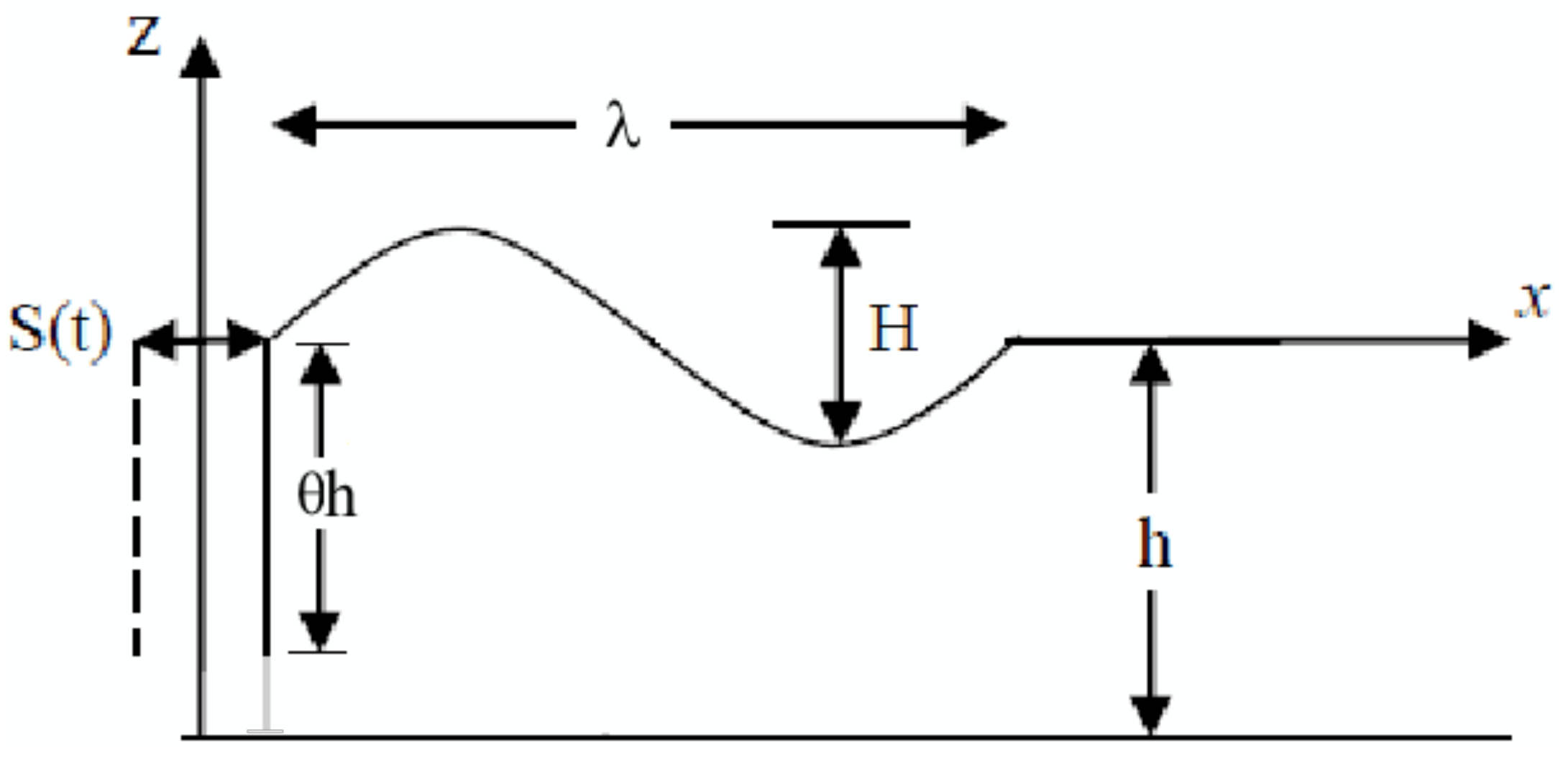
This is conducted by the geometrical modification of the conventional shape of the classic piston wavemaker by a limited depth $\theta$ h to better match the kinematic velocity profile of the wave to be generated, resulting in the proposed wavemaker shown in Figure 1. Such depth is correlated to the wave conditions to be generated, providing an optimization framework for the proper piston dimensions.

Assuming that the displaced water by a single stroke of a wavemaker is equal to the accumulated water in the resulted wave crest, the relation between the wavemaker stroke and the resulted wave height (H/S) may be expressed by equating the displaced water by a full stroke to the volume under the wave crest, as shown in Figure 1, as follows:

$$S\theta h={{\displaystyle \int }}_0^{\lambda /2}\left(\frac{H}{2}\right)sin\left(kx\right)dx=H/k$$

(15)

$${\frac{H}{S}}_{|piston}=\theta kh$$

(16)

which is a valid approximation for relative depths of the shallow-water conditions, i.e., in the range h₀/λ < 0.05. Of course, when θ = 1, the step wavemaker reduces to the simplified conventional piston wavemaker equation.

Complete Theory for Plane Wavemakers—Intermediate-Waters

Assuming that waves are of small-amplitude, long-crested, propagating in a potential and incompressible continuum, the governing equation for the velocity potential, in the geometry depicted in Figure 1, is given by:

$${\phi }_{xx}+{\phi }_{zz}=0$$

(17)

The dynamic and kinematic free surface boundary conditions are:

$$\eta =\frac{1}{g}{\phi }_t, \mathrm{at} z =0,$$

(18)

$$-{\phi }_z={\eta }_t, \mathrm{at} z =0$$

(19)

and the impermeable bottom boundary condition is

$$-{\phi }_z=0, \mathrm{at} z =-h$$

(20)

In the positive x-direction, the horizontal displacement of the stroke wavemaker profile S(z) is described as follows:

$$x=\frac{S\left(z\right)}{2}\mathit{sin}\left(\omega t\right)$$

(21)

The function that describes the surface of the wavemaker is [38]:

$$F\left(x,z,t\right)=x-\frac{S\left(z\right)}{2}\mathit{sin}\left(\omega t\right)=0$$

(22)

As the surface of the wavemaker varies with time, then the total derivative of the surface with respect to time will be zero, i.e.,

$$\frac{dF\left(x,z,t\right)}{dt}=\frac{\partial F}{dt}+u\frac{\partial F}{dx}+w\frac{\partial F}{dz}=0$$

(23)

$$-\frac{\partial F}{dt}=u.\nabla F=u.n\left|\nabla F\right|$$

(24)

The general boundary condition is then:

$$u.n=-\frac{\partial F/\partial t}{\left|\nabla F\right|} , \mathrm{on} F\left(x,z,t\right)=0$$

(25)

where $u=ui+wk$, $n=\nabla \mathrm{F}/\left|\nabla \mathrm{F}\right|$, and $\left|\nabla F\right|=\sqrt{{\left(F_x\right)}^2+{\left(F_{\mathrm{z}}\right)}^2}$.

Substituting F(x,z,t) yields:

$$u\left(0,z,t\right)-\frac{w}{2}\frac{dS\left(z\right) }{dz}\mathit{sin}\left(\omega t\right)=\frac{S\left(z\right)}{2}\omega cos\left(\omega t\right), \mathrm{on} F\left(x,z,t\right)=0$$

(26)

Then, if the wavemaker displacement is considered to be relatively small, the kinematic boundary condition at the wavemaker can be linearized by neglecting the second term on the left hand; hence:

$$u\left(0,z,t\right)=\frac{S\left(z\right)}{2}\omega cos\left(\omega t\right)$$

(27)

The final form of the Laplace equation satisfying the upper and lower boundary conditions is written as follows [38]:

$$\phi =A_{p}cosh\left[k_p\left(h+z\right)\right]sin\left(k_{p}x-\omega t\right)+{\displaystyle \sum }_{n=1}^{\infty }{C}_n{e}^{-k_s\left(n\right)x}cos\left[k_s\left(n\right)\left(h+z\right)\right]cos\left(\omega t\right)$$

(28)

where $A_p$ and $C_n$ are the coefficients to be determined, and the subscripts p and s mean progressive and standing waves generated by the wavemaker, respectively. The standing wave decay exponentially in the x-direction and are negligible two or three water depths away from the wavemaker. Taking into account the kinematic boundary condition at the wavemaker,

$$u\left(0,z,t\right)=\frac{S\left(z\right)}{2}\omega cos\left(\omega t\right)=-{\phi }_x\left(0,z,t\right)$$

(29)

Deriving Equation (28) with respect to x_space and substituting in Equation (29), we obtain Equation (30):

$$\frac{S\left(z\right)}{2}\omega =-A_p{k}_{p}cosh\left[k_p\left(h+z\right)\right]+{\displaystyle \sum }_{n=1}^{\infty }{C}_n{k}_s\left(n\right)cos\left[k_s\left(n\right)\left(h+z\right)\right]$$

(30)

Knowing that, due to the orthogonality property, there is no contribution from the series terms, multiplying Equation (30) by $cosh\left[k_p\left(h+z\right)\right]$ and taking into account that the stroke of the wavemaker S(z) is limited by the water depth, that is $\theta$h, and assuming the functional form of S(z) = $S$ (piston motion) to better match the kinematic velocity profile of the wave in shallow- and intermediate-water conditions, the solution for $A_p$ is obtained by integration of:

$$A_p=-\frac{{{\displaystyle \int }}_{-\theta h}^0\frac{S\left(z\right)}{2}\omega cosh\left[k_p\left(h+z\right)\right]dz}{k_p{{\displaystyle \int }}_{-\theta h}^{0}cos{h}^2\left[k_p\left(h+z\right)\right]dz}$$

(31)

with

$$\int \frac{S\left(z\right)}{2}\omega cosh\left[k_p\left(h+z\right)\right]dz=\frac{S\omega }{2k_p} sinh\left[k_p\left(h+z\right)\right]+C$$

(32)

$$k_p\int cos{h}^2\left[k_p\left(h+z\right)\right] dz=\frac{1}{4}sinh\left[2k_p\left(h+z\right)\right]+\frac{1}{2}{k}_p\left(h+z\right)+C$$

(33)

By integrating between $-\theta h$ and 0, the following expression for $A_p$ is obtained:

$$A_p=-\frac{S\omega \left\{sinh\left(k_{p}h\right)-sinh\left[k_{p}h\left(1-\theta \right)\right]\right\}/\left(2k_p\right)}{\frac{1}{4}sinh\left(2k_{p}h\right)-\frac{1}{4}sinh\left[2k_{p}h\left(1-\theta \right)\right]+\frac{1}{2}{k}_p\theta h}$$

(34)

On the other hand, according to the boundary condition at z = 0 [Equation (18)], the progressive wave height can be linked to the wavemaker as follows:

$$\mathrm{\eta }=\frac{1}{g}{\varphi }_t=\frac{H}{2}cos\left(k_{p}x-\omega t\right)$$

(35)

that is,

$$H=-\frac{2A_p}{g}\omega cosh\left(k_{p}h\right)$$

(36)

The wave-height-to-stroke ratio is finally obtained by substitution of $A_p$ into Equation (36). Taking into account the dispersion relation ${\omega }^2=g{k}_{p}tanh\left(k_{p}h\right),$ the following Equation (37) is obtained:

$${\frac{H}{S}}_{|piston}=\frac{4 sinh\left(k_{p}h\right)\left\{sinh\left(k_{p}h\right)-sinh\left[k_{p}h\left(1-\theta \right)\right]\right\}}{sinh\left(2k_{p}h\right)-sinh\left[2k_{p}h\left(1-\theta \right)\right]+2k_p\theta h}$$

(37)

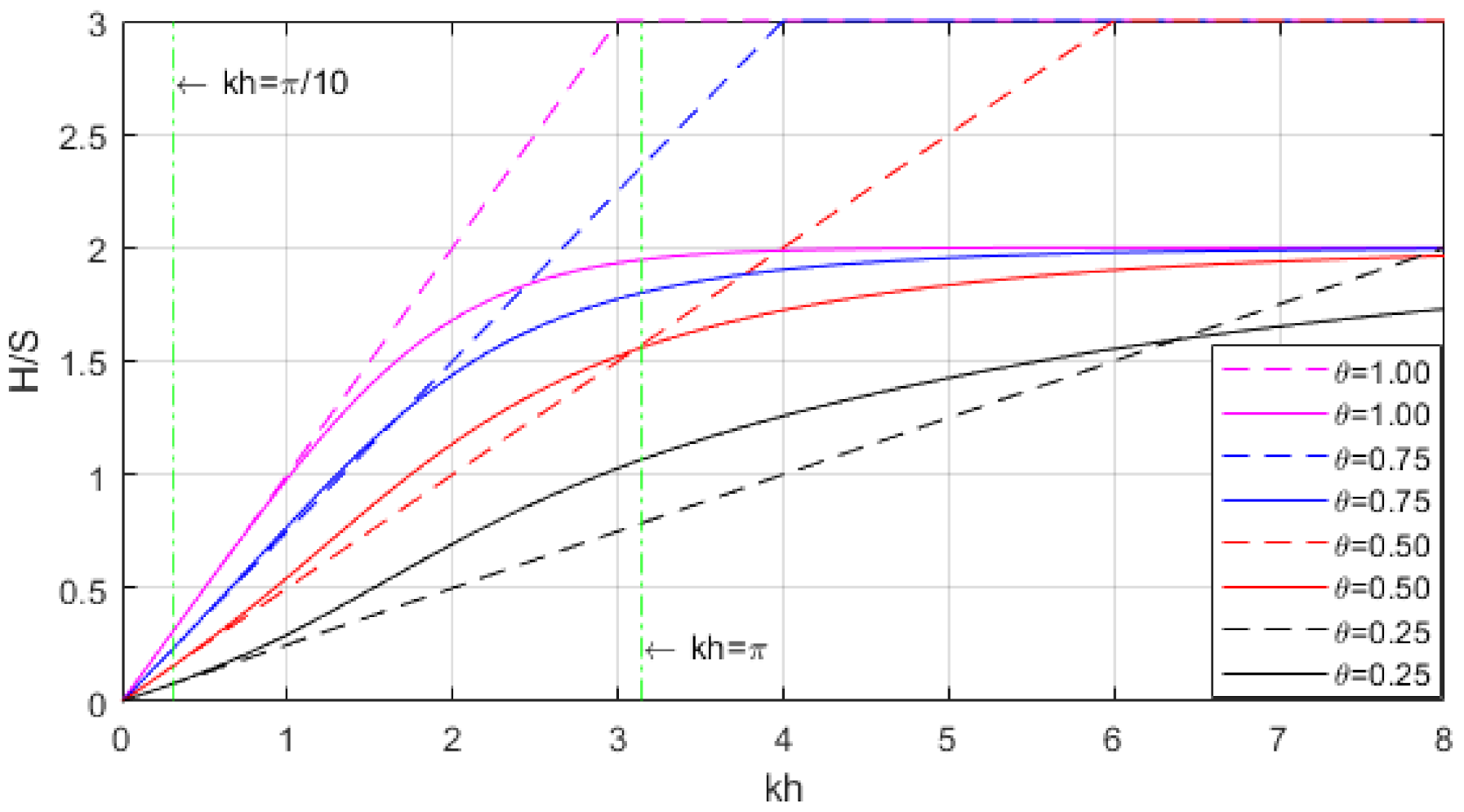
A graphical representation of Equations (16) and (37) for different values of $\theta$ is depicted in Figure 2 (hereafter $k_p=k$). A great difference between both solutions is clear, especially in intermediate and deeper water conditions. Indeed, Equation (16) is not suitable in that range of wave conditions. Even for $\theta$ = 1, the differences start to increase from kh = 1.0. Therefore, our goal is to obtain a correct value for H/S in intermediate-depths. The mean profile of the active velocity in a $\theta$ h portion of the wave generator is expected to better match the orbital velocity profile of a progressive kinematic wave in intermediate-waters compared to the uniform kinematics profile in shallow-waters.

Figure 2 also shows that the maximum value of the relation between the wavemaker stroke and the resulted wave height (H/S) is two, which is obtained in deep-waters (kh > π) and for any value of $\theta$.

Assuming shallow-water conditions within the Airy wave theory for 2D waves, the horizontal water particle velocities are constant along the vertical axis, and the input boundary condition is implemented as follows:

$$u\left(0,t\right)=\sqrt{\frac{g}{h}}\eta \left(0,t\right)$$

(38)

where $\eta \left(0,t\right)=h\left(0,t\right)-\left[{\zeta }_0-\xi \left(x\right)\right]=h\left(0,t\right)-h_0$ is the free surface elevation along the inlet boundary. However, this approach is not valid beyond the conventional shallow-water limit.

A better estimate for the input wave that satisfies the desired value of kh can be obtained considering an optimal value of $\theta$, according to Condition (36). Once obtained $\theta$, the mean wave velocity at the input is given by:

$$u\left(0,t\right)=\frac{C}{\theta h}\eta \left(0,t\right)=\frac{C}{\theta h}\frac{H}{2}cos\left(\omega t\right)=\frac{g}{\theta h\omega }tangh\left(kh\right)\frac{H}{2}cos\left(\omega t\right)$$

(39)

On the other hand, given that,

$$\frac{g}{\theta h\omega }tangh\left(kh\right)\frac{H}{2}cos\left(\omega t\right)=\frac{S\left(z\right)}{2}\omega cos\left(\omega t\right)$$

(40)

the precedent Equation (16) is retrieved:

$${\frac{H}{S}}_{|piston}=\theta h\frac{{\omega }^2}{g tangh\left(kh\right)}=\theta kh$$

(41)

At the outgoing wave boundary, the Sommerfeld radiation condition in Equation (42) is used to allow the passage and output of wave energy, i.e.,

$${\eta }_t+C{\eta }_x=0$$

(42)

where the partial derivative in space of the surface elevation is computed using a second-order backward difference approximation:

$${\eta }_x{}_{|i=N,t}=\frac{3{\eta }_N^t-4{\eta }_{N-1}^t+{\eta }_{N-2}^t}{2\Delta x}$$

(43)

3.3. Wave Breaking Strategy

Taking advantage of a solving methodology, which encompasses the Serre and Saint-Venant systems of equations, the wave-breaking strategy detailed in [26] is used, which consists of switching locally from the system of Serre equations to the Saint-Venant equations when the wave is about to break. Breaking is easily incorporated simply by ignoring the contribution of the dispersive terms included in the parameter ${\sigma }^2$ of Equation (3) (see [26] for details).

4. Results and Discussion

In order to test the robustness of Model (12), several numerical tests were performed. Its good performance is proven through very demanding applications, namely: A1: a solitary wave propagating in a channel 1.0 m depth and 250 m long, with $a/h_0=0.60$; A2: a periodic wave propagating over a submerged bar in shallow-depth (h₀/λ $\approx 0.03$) and intermediate-depth waters (h₀/λ ≈ 0.11); and A3: periodic wave propagating in quasi-deep-water conditions (h₀/λ = 0.50).

4.1. Solitary Wave

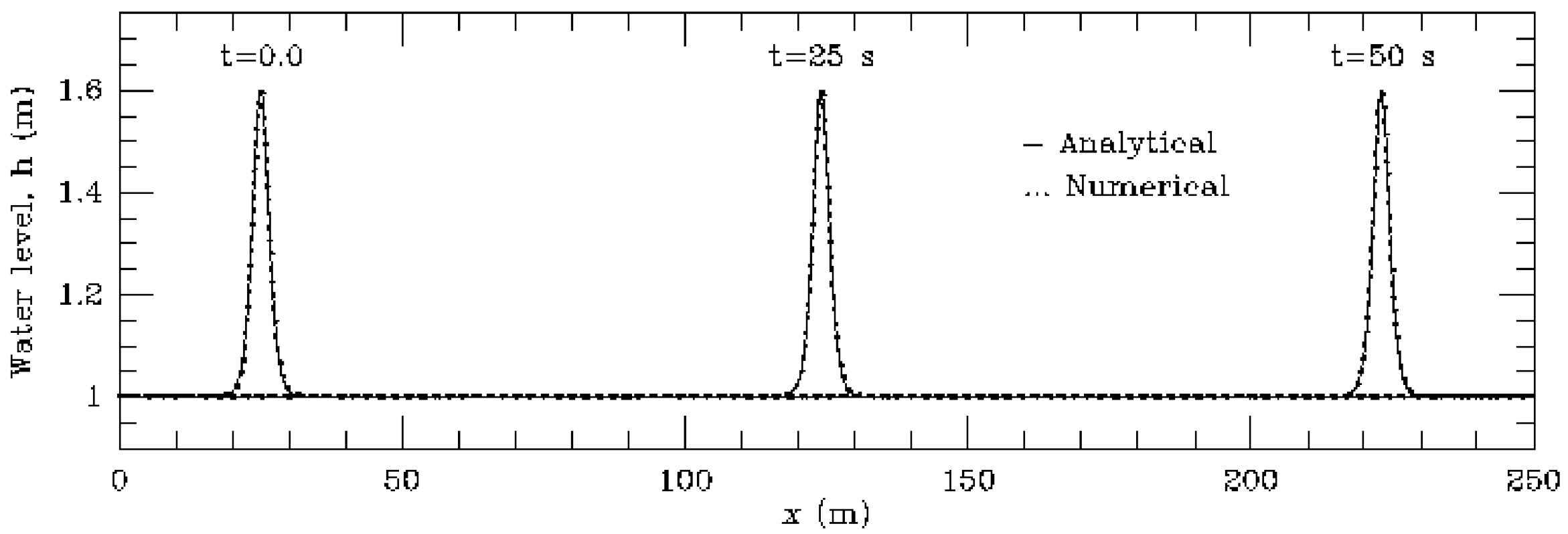
To validate System (12) and check the accuracy of the numerical method used with $\alpha =\beta =0$ and ${\xi }_t={\xi }_x={\xi }_{xx}={\xi }_{xxx}=0$, a comparison with a closed-form solitary wave solution of the Serre equations was made, which is expressed as:

$$h \left(x,t\right)=h_0+a sec{h}^2\left[K\left(x-Ct-x_0\right)\right]$$

(44)

$$u=C\left(1-h_0/h\right)$$

(45)

with

$$K=\sqrt{3a/\left[4h_0^2\left(h_0+a\right)\right]}; C=C_0 \sqrt{1+a/h_0}, \mathrm{and} C_0=\sqrt{g{h}_0}$$

where $h_0$ is the water depth at rest, $x_0$ is the initial position of the crest, and $a$ is the wave amplitude. Constant depth $h_0=1.0$ m and $x_0=25$ m were used. The computational domain was uniformly discretized with a spatial step of $\mathsf{\Delta }x=0.05$ m. A time step of $\mathsf{\Delta }t=0.0025$ s was used. A comparison of the numerical results with the analytical solution in Equations (44) and (45) for the propagation of a solitary wave, where $a/h_0=0.60$, is plotted in Figure 3 at times t = 25 s and t = 50 s. It is possible to observe a perfect agreement, which confirms the accuracy of the numerical model implemented.

4.2. Periodic Wave Propagating over a Sybmerged Bar

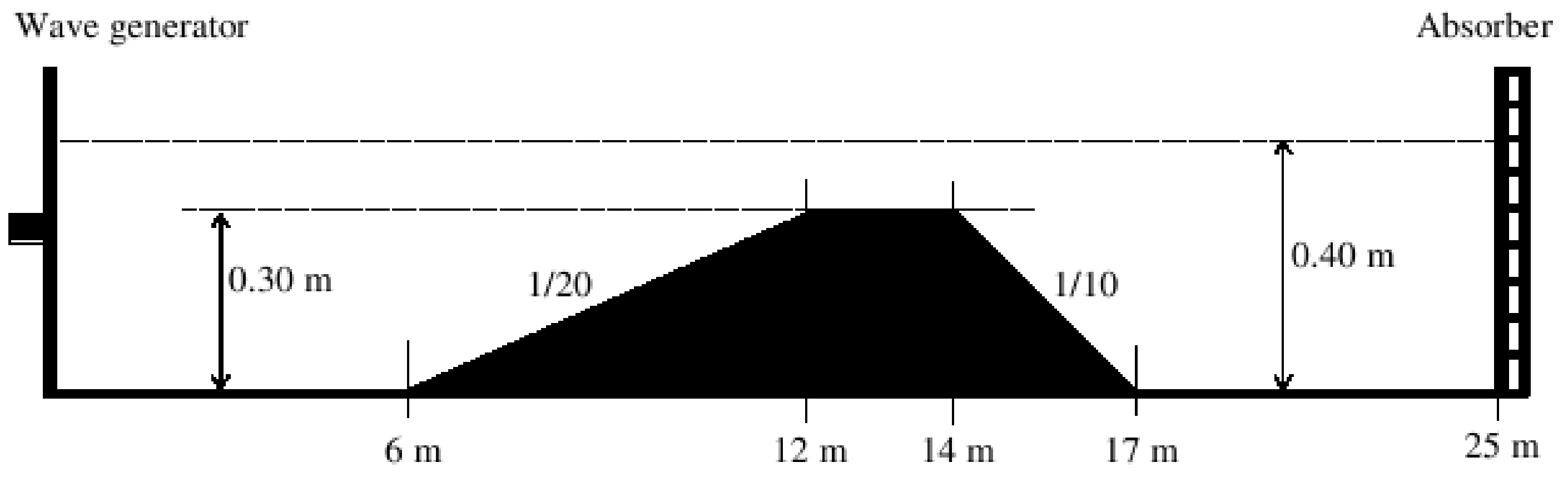
Experimental data are available in the literature and can be used for comparisons. Beji and Battjes [39] carried out experiments in a 0.80 m wide channel with a submerged trapezoidal bar and 1:20 slopes (upstream) and 1:10 (downstream). As shown in Figure 4, the water depth in front of and behind the bar was 0.40 m and only 0.10 m above the bar.

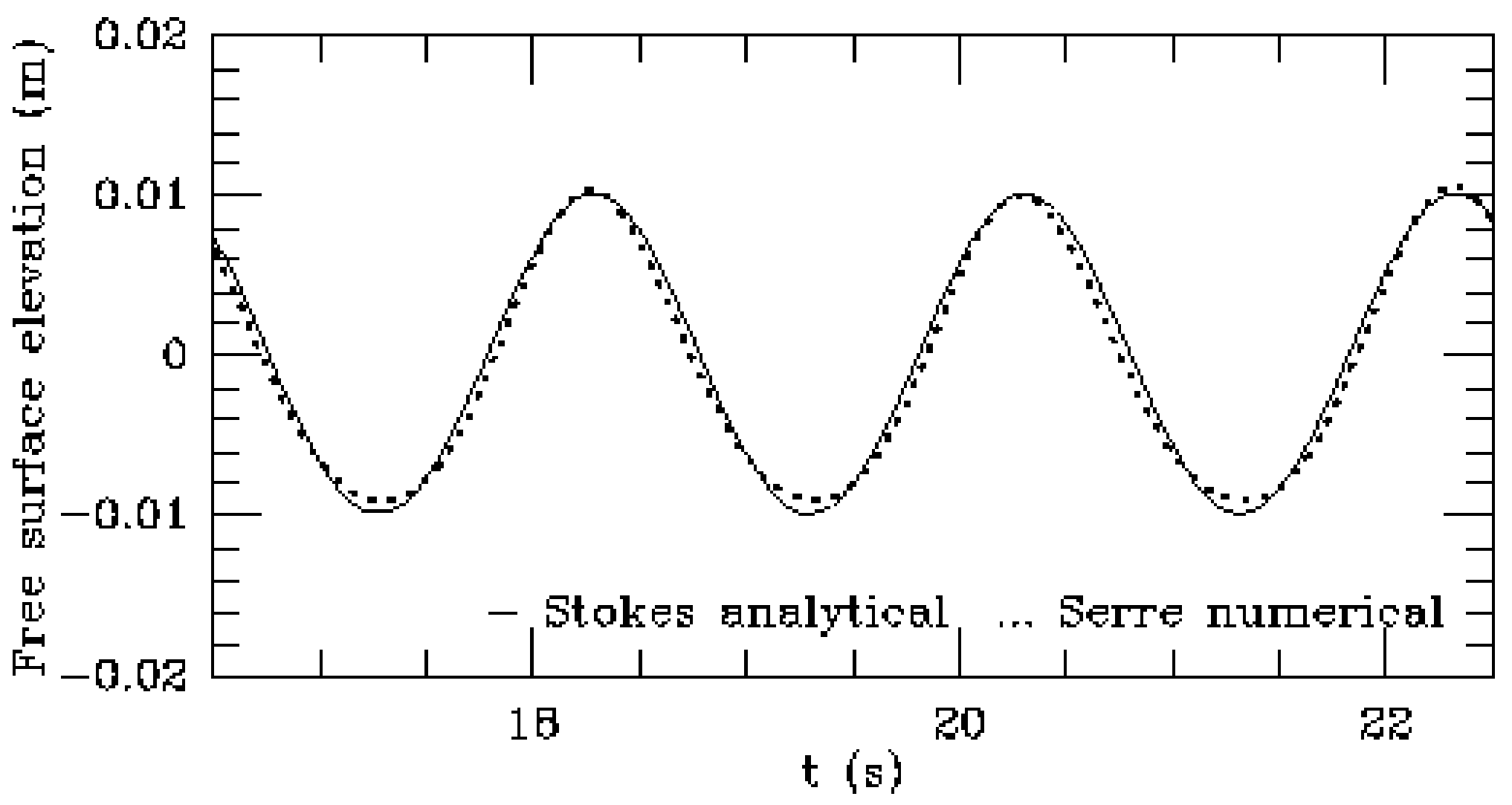
The propagation of a regular wave with a height of 0.02 m, period T = 2.02 s, and wavelength of 3.73 m was simulated. Three wave gauges were placed at the points where the wave nonlinearity and dispersity effects were mostly manifested. The numerical results obtained in a fourth gauge installed at x = 3.0 m were compared with Stokes 2nd order analytical solution.

At the inlet section and during the first 6 m (Figure 4), the relation h₀/λ $\approx 0.107$ was verified, thus satisfying the Stokes solution of the second order in this stretch, while the reflection effects were not felt. According to the theory of second-order Stokes, the elevation of the free surface is given by Equation (46) [40]:

$$\eta =\frac{ H}{2}\cos \left(kx-\omega t\right)+\frac{\pi H^2}{8 \lambda }\left\{\frac{cosh\left(k{h}_0\right) \left[2+cosh\left(2k{h}_0\right)\right]}{sin{h}^3\left(k{h}_0\right)}\right\}\cos \left[2\left(kx-\omega t\right)\right]$$

(46)

The ($u$,$w$) velocity components are:

$$\begin{array}{c}u=\frac{\pi H}{T}\frac{cosh\left[k\left(h_0+z\right)\right]}{cosh\left(k{h}_0\right)}\mathit{cos}\left(kx-\omega t\right)\hfill \\ \hspace{1em}\hspace{1em}\hspace{1em}\hspace{1em}\hspace{1em} +\frac{3}{4}\frac{\pi H}{T}\frac{\pi H}{\lambda }\frac{cosh\left[2k\left(h_0+z\right)\right]}{sin{h}^4\left(k{h}_0\right)}\mathit{cos}\left[2\left(kx-\omega t\right)\right]\hfill \end{array}$$

(47)

$$\begin{array}{c}w=\frac{\pi H}{T}\frac{sinh\left[k\left(h_0+z\right)\right]}{cosh\left(k{h}_0\right)}sin\left(kx-\omega t\right)\hfill \\ \hspace{1em}\hspace{1em}\hspace{1em}\hspace{1em}\hspace{1em} +\frac{3}{4}\frac{\pi H}{T}\frac{\pi H}{\lambda }\frac{sinh\left[2k\left(h_0+z\right)\right]}{sin{h}^4\left(k{h}_0\right)}sin\left[2\left(kx-\omega t\right)\right]\hfill \end{array}$$

(48)

where $H$ is the wave height, k = 2π/λ is the wave number, and $\omega =2\pi /T$ is the wave frequency. Using $z=0,$ the velocity at the surface is obtained. The computational domain was discretized with a uniform grid spacing of $\mathsf{\Delta }x=0.025$ m. A time step of $\mathsf{\Delta }t=0.0010$ s was used. A comparison of the analytical solution in Equation (46) with the numerical results of the Serre model in Equation (12) is shown in Figure 5.

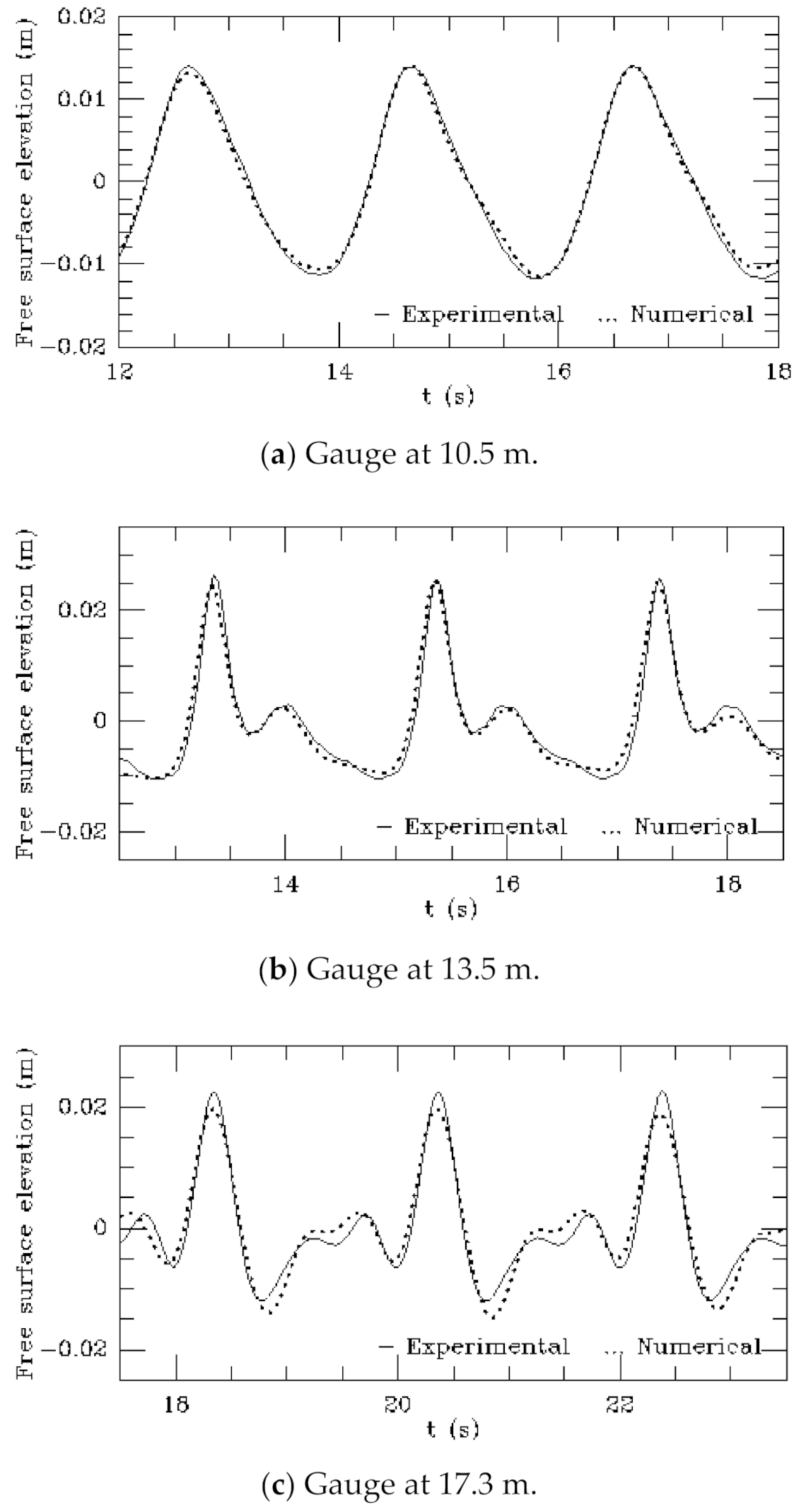
Additionally, the numerical results are compared with the data recorded in probes installed at x = 10.5 m, x = 13.5 m, and x = 17.3 m (Figure 4); these comparisons are shown in Figure 6a–c.

Despite some discrepancies, the numerical results of the Serre model with improved dispersive characteristics agree satisfactorily with the measured data. It should be noted that Serre’s standard equations are unable to reproduce the input and propagation of a wave under these conditions, given that h₀/λ is greater than 0.09. In this case, with h₀/λ $\approx 0.11$ ($k{h}_0\approx 0.67$), the error could be significant.

4.3. Periodic Wave Propagating in Quasi-Deep-Water Conditions (h₀/λ = 0.50)

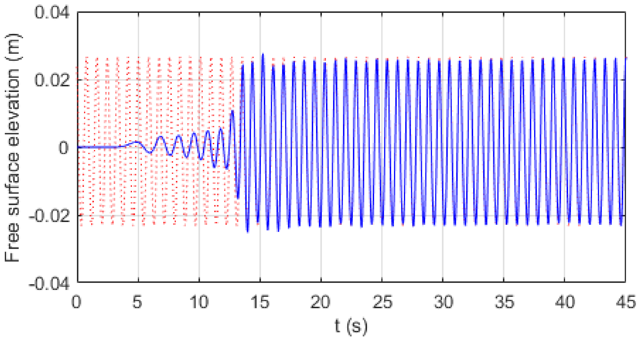
In order to evaluate the performance of the improved Serre model [System of Equation (12)] in quasi-deep-water conditions the input and propagation of a periodic wave in an initially undisturbed region of constant depth $h_0=0.56$ m is tested. The wave characteristics are amplitude a = 0.025 m, period T = 0.85 s, and wavelength λ = 1.12 m; therefore, h_0/λ = 0.5 $\left(k{h}_0=\pi \right)$. At the input boundary, Relation (39) is implemented, which is equivalent to Equation (49), as addressed earlier in the theoretical analysis section:

$$u\left(0,t\right)=\frac{g}{\omega }\frac{\mathit{tanh}\left(kh\right)}{\theta h} \eta \left(0,t\right)$$

(49)

where $\theta =0.960$, $h=h_0$ and $\eta \left(0,t\right)=a\mathit{cos}\left(\omega t\right)$.

The computational domain was discretized using a constant space step $\mathsf{\Delta }x=0.05$ m. A time step of $\mathsf{\Delta }t=0.010$ s meets the stability condition. Figure 7 shows a comparison of the analytical Stokes solution of the second-order Equation (46) with the numerical results of the free surface profile at x = 10 m. A steady periodic flow was established, confirming the good performance of the numerical model in quasi-deep-water conditions. It should be noted that Serre’s Equation (5) is not capable of reproducing these conditions.

5. Conclusions

Serre’s standard equations are only valid for shallow-water conditions; therefore, it becomes necessary to develop an extension of these equations for applications at intermediate-depths and quasi-deep-waters. In fact, these are the conditions that a wave experiences when propagating from offshore to very shallow-water conditions. Accordingly, a new computational structure is proposed in this work, composed of a set of Serre equations enhanced with additional terms of dispersive origin. The applications carried out clearly demonstrate the capacity of this computational structure to simulate the phenomena experienced by waves as they propagate from offshore to very shallow-waters.

The robustness of the computational structure is tested through applications in intermediate-water depths and on bathymetry with considerable slopes. It is shown that Serre’s equations extended with additional terms of dispersive origin are capable of propagating waves from quasi-deep-waters, as long as $\sigma \le$ 0.05, such as tidal waves and tsunamis, to very shallow-waters.

Regarding boundary conditions, it is shown that the solution commonly used in shallow-water conditions within the Airy wave theory is not valid in deeper waters. Based on the wavemaker theory, a solution is proposed for the inlet boundary considering a limited depth $\theta h$ for the piston wavemaker.

Further studies should allow obtaining the optimal $\theta$ values to be considered in the input boundary condition for applications of the model in the entire range of intermediate-waters. This same condition must be analyzed for the output boundary with free wave output or to fix possible reflection percentage values (Dirichlet condition). An extended version of Serre’s two-dimensional equation system shown in System (4) with improved linear dispersion characteristics, using a finite volume method, is currently being developed and will be published soon.

References

- Berkhoff, J.; Booij, N.; Radder, A. Verification of numerical wave propagation models for simple harmonic linear water waves. Coast. Eng. 1982, 6, 255–279. [Google Scholar] [CrossRef]
- Kirby, J.T.; Dalrymple, R.A. A parabolic equation for the combined refraction–diffraction of Stokes waves by mildly varying topography. J. Fluid Mech. 1983, 136, 435–466. [Google Scholar] [CrossRef] [Green Version]
- Booij, N. A note on the accuracy of the mild-slope equation. Coast. Eng. 1983, 7, 191–203. [Google Scholar] [CrossRef]
- Kirby, J.T. A note on linear surface wave-current interaction over slowly varying topography. J. Geophys. Res. Space Phys. 1984, 89, 745. [Google Scholar] [CrossRef]
- Dalrymple, R.A. Model for Refraction of Water Waves. J. Waterw. Port Coastal Ocean Eng. 1988, 114, 423–435. [Google Scholar] [CrossRef]
- Carmo, J.S.A.D. Wave–current interactions over bottom with appreciable variations in both space and time. Adv. Eng. Softw. 2010, 41, 295–305. [Google Scholar] [CrossRef]
- Saint-Venant, B. Theory of unsteady water flow, with application to river floods and to propagation of tides in river channels. Computes Rendus. Acad. Sci. 1871, 73, 237–240. [Google Scholar]
- Seabra-Santos, F.J. Contribution a L’ètude des Ondes de gravité Bidimensionnelles en eau Peu Profonde. Ph.D. Thesis, Université Scientifique et Médicale et Institut National Polutechnique de Grenoble, Grenoble, France, 1985, unpublished (In French). [Google Scholar]
- Boussinesq, J. Théorie des ondes et des remous qui se propagent le long d’un canal rectangulaire horizontal. J. Mathématiques Pures Appliquées 1872, 17, 55–108. [Google Scholar]
- Serre, F. Contribution à l’étude des écoulements permanents et variables dans les canaux. Houille Blanche 1953, 39, 374–388. [Google Scholar] [CrossRef] [Green Version]
- Green, A.E.; Naghdi, P.M. A derivation of equations for wave propagation in water of variable depth. J. Fluid Mech. 1976, 78, 237–246. [Google Scholar] [CrossRef]
- Antunes do Carmo, J.S.; Seabra-Santos, F.J. On breaking waves and wave-current interaction on shallow water: A 2DH finite element model. Int. J. Num. Meth. Fluids 1996, 22, 429–444. [Google Scholar] [CrossRef]
- Bonneton, P.; Barthelemy, E.; Chazel, F.; Cienfuegos, R.; Lannes, D.; Marche, F.; Tissier, T. Recent advances in Serre–Green Naghdi modelling for wave transformation, breaking and runup processes. Eur. J. Mech. B Fluids 2011, 30, 589–597. [Google Scholar] [CrossRef]
- Filippini, M.; Kazolea, A.G.; Ricchiuto, M. A flexible genuinely nonlinear approach for nonlinear wave propagation, breaking and run-up. J. Comput. Phys. 2016, 310, 381–417. [Google Scholar] [CrossRef]
- Carmo, A.d.J.S.; Seabra-Santos, F.J.; Amado-Mendes, P. Sudden bed changes and wave–current interactions in coastal regions. Adv. Eng. Softw. 2002, 33, 97–107. [Google Scholar] [CrossRef]
- Pitt, J.P.A.; Zoppou, C.; Roberts, S.G. Behaviour of the Serre equations in the presence of steep gradients revisited. Wave Motion 2018, 76, 61–77. [Google Scholar] [CrossRef] [Green Version]
- Zoppou, C.; Pitt, J.; Roberts, S.G. Numerical solution of the fully non-linear weakly dispersive serre equations for steep gradient flows. Appl. Math. Model. 2017, 48, 70–95. [Google Scholar] [CrossRef]
- Tissier, M.; Bonneton, P.; Marche, F.; Chazel, F.; Lannes, D. A new approach to handle wave breaking in fully non-linear Boussinesq models. Coast. Eng. 2012, 67, 54–66. [Google Scholar] [CrossRef]
- Kazolea, M.; Ricchiuto, M. On wave breaking for Boussinesq-type models. Ocean Model. 2018, 123, 16–39. [Google Scholar] [CrossRef] [Green Version]
- Carmo, J.S.A.D.; Ferreira, J.A.; Pinto, L. On the accurate simulation of nearshore and dam break problems involving dispersive breaking waves. Wave Motion 2019, 85, 125–143. [Google Scholar] [CrossRef]
- Nwogu, O. Alternative Form of Boussinesq Equations for Nearshore Wave Propagation. J. Waterw. Port. Coastal. Ocean Eng. 1993, 119, 618–638. [Google Scholar] [CrossRef] [Green Version]
- Gobbi, M.; Kirby, J.; Wei, G. A fully nonlinear Boussinesq model for surface waves. Part 2. Extension to O(kh)4. J. Fluid Mech. 2000, 405, 181–210. [Google Scholar] [CrossRef] [Green Version]
- Carmo, J.S.A.D. Boussinesq and Serre type models with improved linear dispersion characteristics: Applications. J. Hydraul. Res. 2013, 51, 719–727. [Google Scholar] [CrossRef]
- Lannes, D.; Marche, F. A new class of fully nonlinear and weakly dispersive Green–Naghdi models for efficient 2D simulations. J. Comput. Phys. 2015, 282, 238–268. [Google Scholar] [CrossRef] [Green Version]
- Clamond, D.; Dutykh, D.; Mitsotakis, D. Conservative modified Serre–Green–Naghdi equations with improved dispersion characteristics. Commun. Nonlinear Sci. Numer. Simul. 2017, 45, 245–257. [Google Scholar] [CrossRef] [Green Version]
- Antunes do Carmo, J.S.; Ferreira, J.A.; Pinto, L.; Romanazzi, G. An improved Serre model: Efficient simulation and comparative evaluation. Appl. Math. Model. 2018, 56, 404–423. [Google Scholar] [CrossRef]
- Antunes do Carmo, J.S.; Seabra-Santos, F.J.; Barthélemy, E. Surface waves propagation in shallow water: A finite element model. Int. J. Numer. Methods Fluids 1993, 16, 447–459. [Google Scholar] [CrossRef]
- Lynett, L.; Liu, P.L.-F. Modeling Wave Generation, Evolution, and Interaction with Depth Integrated, Dispersive Wave Equations COULWAVE Code Manual; Cornell University Long and Intermediate Wave Modeling Package; Cornell University: Ithaca, NY, USA, 2002. [Google Scholar]
- Tonelli, M.; Petti, M. Hybrid finite volume–finite difference scheme for 2DH improved Boussinesq equations. Coast. Eng. 2009, 56, 609–620. [Google Scholar] [CrossRef]
- Chazel, F.; Lannes, D.; Marche, F. Numerical Simulation of Strongly Nonlinear and Dispersive Waves Using a Green–Naghdi Model. J. Sci. Comput. 2011, 48, 105–116. [Google Scholar] [CrossRef] [Green Version]
- Mitsotakis, D.; Synolakis, C.; McGuinness, M. A modified Galerkin/finite element method for the numerical solution of the Serre-Green-Naghdi system. Int. J. Numer. Methods Fluids 2017, 83, 755–778. [Google Scholar] [CrossRef]
- Seabra-Santos, F.J. As aproximações de Wu e de Green & Naghdi no quadro geral da teoria da água pouco profunda. In Proceedings of the Simpósio Luso-Brasileiro de Hidráulica e Recursos Hídricos (4° SILUSBA) 209–219, Lisbon, Portugal, 14–16 June 1989, unpublished (In Portuguese). [Google Scholar]
- Antunes do Carmo, J.S. Nonlinear and dispersive wave effects in coastal processes. Management 2016, 16, 343–355. [Google Scholar] [CrossRef] [Green Version]
- Antunes do Carmo, J.S. Modeling of wave propagation from arbitrary depths to shallow waters-A review. In New Perspectives in Fluid Dynamics; Chaoqun, L., Ed.; InTech-Open Access Publisher: London, UK, 2015; pp. 23–66. [Google Scholar] [CrossRef] [Green Version]
- Madsen, P.A.; Sørensen, O.R. A new form of the Boussinesq equations with improved linear dispersion characteristics. Part A slowly-varying bathymetry. Coast. Eng. 1992, 18, 183–204. [Google Scholar] [CrossRef]
- Beji, S.; Nadaoka, K. A formal derivation and numerical modelling of the improved Boussinesq equations for varying depth. Ocean Eng. 1996, 23, 691–704. [Google Scholar] [CrossRef]
- Liu, Z.B.; Sun, Z.C. Two sets of higher-order Boussinesq-type equations for water waves. Ocean Eng. 2005, 32, 1296–1310. [Google Scholar] [CrossRef]
- Dean, R.G.; Dalrymple, R.A. Water Wave Mechanics for Engineers and Scientists 1984; Prentice-Hall, Inc.: Englewood Cliffs, NJ, USA, 1984; ISBN 0-13-946038-1. [Google Scholar]
- Beji, S.; Battjes, J.A. Experimental investigation of wave propagation over a bar. Coast. Eng. 1993, 19, 151–162. [Google Scholar] [CrossRef]
- Carmo, J.S.A.D. Processos Físicos e Modelos Computacionais em Engenharia Costeira; Imprensa da Universidade de Coimbra/Coimbra University Press: Coimbra, Portugal, 2016; ISBN 978-989-26-1152-5. [Google Scholar] [CrossRef]
Figure 1.
Schematic diagram of the piston wavemaker reduced to a limited depth h. H is the wave height, λ is the wavelength, h is the water depth, S is the wavemaker stroke, and 1.0 is a parameter.
Figure 2.
Wave height to wavemaker stroke relationship (H/S) in the function of kh. Comparison of Solutions (16) and (37) for different values of .
Figure 3.
Propagation of a solitary wave with . Comparison of the analytic solutions in Equations (32) and (33) () with the numerical results () of the Serre model in Equation (12) with .
Figure 4.
Bathymetry for the periodic wave propagating over the submerged bar (not in scale).
Figure 5.
Periodic wave with 0.02 m height, 2.02 s period, and 3.73 m wavelength propagating in a channel of 0.40 m depth. Comparison of the analytical Stokes 2nd order solution in Equation (46) with numerical results in a gauge installed at x = 3.0 m ().
Figure 6.
Periodic wave propagating over a bar (as shown in Figure 4). Free surface evolution at three gauges installed at (a) x = 10.5 m, (b) x = 13.5 m, and (c) x = 17.3 m.
Figure 7.
Sinusoidal wave with 0.05 m height, 0.85 s period, and 1.12 m wavelength, propagating in a channel of 0.56 m depth. Comparison of the analytical Stokes 2nd-order solution in Equation (46) (red dotted) with the numerical results obtained in a probe installed at x = 10.0 m (blue line).
Publisher’s Note: MDPI stays neutral with regard to jurisdictional claims in published maps and institutional affiliations. |
© 2021 by the author. Licensee MDPI, Basel, Switzerland. This article is an open access article distributed under the terms and conditions of the Creative Commons Attribution (CC BY) license (https://creativecommons.org/licenses/by/4.0/).
Share and Cite
MDPI and ACS Style
Antunes Do Carmo, J.S. Remarks on the Boundary Conditions for a Serre-Type Model Extended to Intermediate-Waters. Modelling 2021, 2, 626-640. https://0-doi-org.brum.beds.ac.uk/10.3390/modelling2040033
AMA Style
Antunes Do Carmo JS. Remarks on the Boundary Conditions for a Serre-Type Model Extended to Intermediate-Waters. Modelling. 2021; 2(4):626-640. https://0-doi-org.brum.beds.ac.uk/10.3390/modelling2040033
Chicago/Turabian StyleAntunes Do Carmo, José Simão. 2021. "Remarks on the Boundary Conditions for a Serre-Type Model Extended to Intermediate-Waters" Modelling 2, no. 4: 626-640. https://0-doi-org.brum.beds.ac.uk/10.3390/modelling2040033