
A Lagrangian Tool for Simulating the Transport of Chemical Pollutants in the Arabian/Persian Gulf


Department Física Aplicada I, ETSIA, Universidad de Sevilla, Carretera de Utrera km 1, D.P. 41013 Seville, Spain
Modelling 2021, 2(4), 675-685; https://doi.org/10.3390/modelling2040036
Submission received: 13 September 2021
/
Revised: 16 November 2021
/
Accepted: 18 November 2021
/
Published: 22 November 2021
(This article belongs to the Special Issue Ocean and Coastal Modelling)
Abstract
:A rapid-response Lagrangian model for the use in simulation of the transport of a chemical pollutant in the Arabian/Persian Gulf is described. The model is well suited to the provision of a fast response after an emergency due to an accident or a deliberate spill. It is easy to set up for any situation since only requires the modification of a few input files specifying the pollutant properties and release characteristics. Running times are short, even on a desktop PC, which makes it appropriate for a rapid assessment of a hypothetical accident occurring in the region. Baroclinic circulation was obtained from an HYCOM ocean model, and tides were calculated using a barotropic model. The interactions of pollutants with sediments (uptake/release processes) were described using a dynamic approach based on kinetic transfer coefficients and a stochastic numerical method. Some examples of model applications are shown, showing the influence of the geochemical behaviour of the pollutant in its distribution patterns.
1. Introduction
Assessments of pollutant concentrations in the environment partially rely on model outputs. Models should describe the main pollutant transport processes within the environment and modelling tools depend on the assessment character, which may be “predictive”, where expected concentrations are estimated for future release scenarios, or “retrospective", where they are estimated for past time sources. The modelling approach can also differ for cases of regular or accidental releases. Three types of pollutant transport models can be applied in the marine environment:
- Box models: In these models, the marine area under consideration is divided into a number of large boxes or compartments. These boxes are interconnected according to water circulation and it is assumed that the transport of pollutants between boxes is proportional to the difference in radionuclide concentration between them. It is assumed that mixing of radionuclides within each box is uniform and instantaneous. These models were widely applied to simulate the transport of radionuclides in the sea [1,2].
- Eulerian models: Differential equations giving the temporal and spatial evolution of the pollutant concentrations in different states (e.g., dissolved in water column and pore water in sediments, fixed on the suspended and bottom sediment etc.) are solved. Some application cases may be seen in [3,4].
- Lagrangian models: In Lagrangian models, the released contaminant is represented by a number of particles, each one equivalent to a given amount of units (kg, moles, etc). The path followed by each particle is calculated and pollutant concentrations are obtained from the number of particles per volume or mass unit. Some examples of applications may be seen in [5,6].
The basic assumptions in box models (uniform and instantaneous mixing of pollutants within each box) make these models well suited to long-term assessments over large spatial scales. Thus, they are useful tools for the environmental assessment of chronic releases from a given industrial facility. Eulerian and Lagrangian models make use of detailed water circulation fields, changing in time and space. Thus, these models provide distributions of contaminants in space and time, which make them appropriate for its use after an accidental release. In particular, Lagrangian models are specially well suited to accidental releases since they do not introduce numerical diffusion [7] and thus can handle the very high concentration gradients between contaminated and clean water, which would be expected after an acute pollutant release into the sea. In addition, computation can be significantly faster than in Eulerian models, where the contaminated area is initially a small part of the whole computational domain, and if the number of particles in the simulation is reasonable (typically a few tens of thousands). A more detailed review of the relative advantages of each modelling approach may be seen in [8].
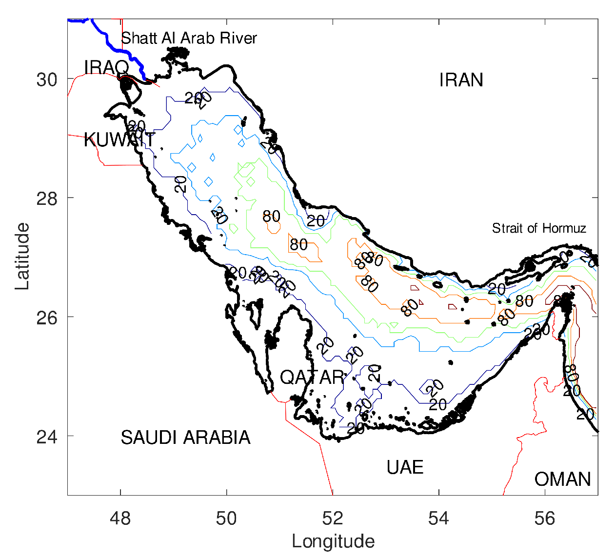
The Arabian (or Persian) Gulf—APG from now on—(Figure 1) is exposed to a number of pollutant threads. This constitutes a significant concern for countries surrounding the APG, since desalination plants are their main freshwater source. In addition, commercial and subsistence fisheries provide a living for a large sector of the coastal population [9].
Some of the sources of pollution [10] include desalination plants (which are a source of radium in the brine discharged to the sea) and phosphate industry (in phosphogypsum waste). Oil spills are relatively common in the APG, in addition to the massive releases during the 1991 Gulf War. In addition to this, the APG, Strait of Hormuz and Gulf of Oman are some of the most important waterways in the world; thus, they are exposed to pollution incidents due to shipping activities. Recently, there has also been growing concern about the nuclear power plants (NPP) which are operating along the APG coasts. There are two operational NPPs in the region, Bushehr in Iran and Barakah in UAE, whose unit 1 was connected to the power grid in summer 2020. About seventeen more are planned in the Kingdom of Saudi Arabia, with the intention for them to be operational by 2030 [11].
Consequently, it is relevant to have a numerical model capable of assessing the effects of pollutant releases (both chemical and radioactive) into the APG. Although some models are described in the literature concerning the dispersion of oil spills in the APG [12], this is not the case for chemical pollutants. The objective of the present model consists of filling such a gap.
APERTRACK is a Lagrangian three-dimensional model which simulates the transport of pollutants in the APG. It can be applied to any chemical pollutant since a decay process is included (which can be due to radioactive decay or another decay process, such as biodegradation). Furthermore, interactions between pollutants and sediments are included in a dynamic way, by means of kinetic transfer coefficients. It is known that heavy metals and some radioactive elements (Pu, Th, etc) present a high affinity to be fixed to sediments; thus, these processes are relevant for these kinds of contaminants.
The model code was written in Fortran, all required input data were open and open source software was used for result visualization. In particular, the scripts provided to draw contaminant concentration maps were developed for GNU Octave, version 5.2.0, free software. Octave is available for Windows and Linux computers. The model with all required input data and scripts for visualization may be downloaded for free from the authors’ webpage https://personal.us.es/rperianez/, accessed on 15 November 2021. The main characteristics are presented in Table 1.
2. Materials and Methods
The conceptual and mathematical model is described in detail in [13,14], and only some indications are given here. The model was Lagrangian; thus, the pollutant release into the sea was simulated by means of a number of particles. Each particle was equivalent to a number of units (for instance Bq, kg, moles, etc), and trajectories were calculated during the simulated period. The transport model considered physical transport (three-dimensional advection due to water currents and three-dimensional mixing due to turbulence) plus decay and interactions of pollutants with bed sediments (adsorption/desorption reactions).
Turbulent mixing, decay and exchanges of contaminants between water and sediment were described through a stochastic method, details of which can be seen in a number of papers (see for instance [15]). Water currents, which are responsible for advective transport, were due to tides, density-driven (baroclinic) circulation and wind.
Exchanges of pollutants between water and sediments were described in a dynamic way using kinetic transfer coefficients. These were deduced from the equilibrium distribution coefficient, , as explained in earlier works (see [4] for instance). The International Atomic Energy Agency (IAEA) [16] provided recommended values for a large number of elements.
Advection due to the current in a Lagrangian model was computed solving the following equation for each particle:
where is time step in the Lagrangian model, and are the changes in particle position , U and U are water velocity components (east–west and south–north directions, respectively) at the particle position and depth and for the corresponding calculation time step, since currents change in time. These currents are the addition of baroclinic currents (downloaded from the HYCOM model) and tidal currents and residuals derived from the tidal model. This is explained below.
The maximum size of the horizontal step given by the particle due to turbulent mixing, , is [15]:
in the direction , where is the horizontal diffusion coefficient (set as 10 m/s) and is an uniform random number between 0 and 1. This equation gives the maximum size of the step. The real size at a given time and for a given particle was obtained by multiplying the equation by another independent random number. This was required to ensure that a Fickian diffusion process was simulated. The time step used to integrate the Lagrangian model was set as s.
Similarly, the size of the vertical step is [15]:
given either upward or downward conditions. is the vertical diffusion coefficient, set as m/s.
Decay of the pollutant was solved with a stochastic method [15] in which decay probability was defined as:
where is the pollutant decay constant. A new random number was generated. If , the particle decayed and was removed from the computation. A similar procedure was used to solve uptake/release processes between water and sediments since they were treated as decay processes from water to sediment or from sediment to water. The constants for these processes were the kinetic transfer coefficients mentioned above, and details of the method may be seen, for instance, in [4,14,15]. Essentially, a kinetic coefficient, , governed adsorption, and a coefficient, , governed desorption. The probability that a dissolved particle is adsorbed by the sediment is:
If a newly generated independent random number was , then the particle was adsorbed by the sediment. The probability that a particle which was fixed to the sediment was redissolved is written as:
and the same procedure followed. is a correction factor that takes into account the fact that part of the sediment surface is hidden by surrounding sediments. Thus, this part did not interact with water.
The number of units corresponding to each particle, R, was deduced from the number of particles in the simulation, , and the magnitude of the release, M:
Then, the concentration of the contaminant in the surface water layer of each grid cell is:
where gives the cell surface, is the number of particles in the surface layer of cell and is the surface layer thickness (thus, we only considered particles at depths less than ). The pollutant inventory in the deep water layer is given by:
where is the number of particles in cell at depths larger than . Finally, concentration in the bed sediment of cell is:
where is the number of particles in the bed sediment of cell , L is sediment thickness and is sediment bulk density:
where kg/m is mineral particle density and is sediment porosity. A number of parameters were defined within the code, whose values were selected from standard ones or previous works. Thus, sediment thickness was defined as m, porosity was set as , the desorption kinetic rate as s, the sediment correction factor as and the water surface layer thickness as m. Of course, these values could be changed if desired.
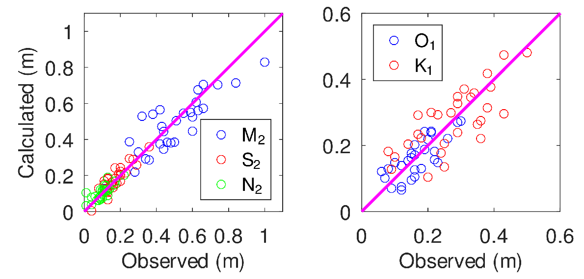
A two-dimensional depth-averaged model was used to simulate tides in the APG. Calculated elevations and currents were treated through standard tidal analysis [17], and tidal constants (amplitudes and phases) were then calculated and stored for each grid cell in the computational domain. Five constituents were considered: three semidiurnal (, and ) and two diurnal ( and ). The Eulerian residual transport was calculated to obtain tidal residual currents [18]. The tidal model was depth-averaged; thus, it provided averaged currents over the water column. A standard current profile was used to generate a vertical structure in the tidal current fields, since these currents decrease from sea surface to the bottom because of friction. Details may be seen in [17], for instance. A comparison between observed [19] and calculated elevations for the five constituents may be seen in Figure 2. If calculated values were linearly fitted to the observed ones, the respective coefficients for the , , , and constituents were 0.7471, 0.7786, 0.6218, 0.5557 and 0.5902. Agreement was generally good; higher discrepancies appeared at some locations, but they were most likely due to the relatively coarse resolution of the model: tides were simulated using the same 0.08 grid as used in the HYCOM model (see below).
Once amplitudes and phases (adapted phase, i.e., for the local time meridian) for each grid cell and constituent (calculated from the tidal analysis) were known, the nodal factor and equilibrium argument of each constituent i at Greenwich were used to evaluate the exact tidal state during each time step of the pollutant simulation and location in the APG. The procedure is described in detail in [20]. Nodal factors and equilibrium arguments for year 2021 were used, meaning that the beginning of this year is . Of course, values for any other year may be used. The main equation was:
where is the location datum, is frequency of constituent i, and are amplitude and phase for the corresponding location (these quantities are obtained from the tidal analysis), is nodal factor and the equilibrium argument of the constituent at Greenwich. Note that the sum extends to 5, since this is the number of included constituents. This same procedure was applied to tidal currents.
The HYCOM (Hybrid Coordinate Ocean Model) [21], model was used to obtain baroclinic circulation in the APG. HYCOM is a primitive equation general circulation model with 40 vertical layers increasing in thickness from the surface to the sea bottom and 0.08 horizontal resolution in both latitude and longitude. Daily current data were obtained from the HYCOM data server (https://www.hycom.org/dataserver, accessed on 15 November 2021).This model was previously used to study circulation in the APG [22].
The domain of the model extends from 23 N to 31 N in latitude, from 47 E to 57 E in longitude, and may be seen in Figure 1. The number of Lagrangian particles in the model is 200,000, which provides a good compromise between accuracy and computational speed. Actually, significant differences in results could not be seen if the number of particles was increased. A simulation over three months takes about 10 minutes on a desktop PC working over the Ubuntu 18.04 operating system.
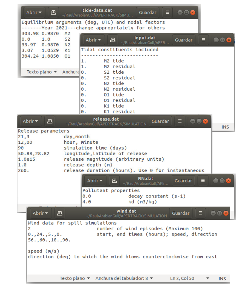
A number of files specify the release characteristics (date, time, position in geographic coordinates, depth, magnitude and duration) and simulation time, pollutant properties (decay constant and equilibrium distribution coefficient (which may be obtained from IAEA [16], as mentioned above), and, finally, an optional wind forecast (see next paragraph) and components of the currents to be used: tidal currents and residuals may be individually switched on and off (to allow comparisons if they are included or not in the simulations or to speed them up by removing tides in the calculations). These switches are provided in a specific file named input.dat. A list of the input files which should be modified for a particular simulation is given in Table 2.
It should be noted that the model can deal with both instantaneous and continuous releases (it was mentioned above that release duration is a required input). In order to simulate a instantaneous release, the release duration must be simply fixed as 0 (zero).
In the case of a simulation to assess the effects of an acute release due to an accident, for instance, it may be relevant to include a local wind, which is considered uniform in the release area. Wind data are provided in a file as a number of different “wind episodes” (any number can be used with a maximum of 100), with each one being characterized by wind speed, direction and start and end times measured in hours after the pollutant release beginning. These time-evolving wind conditions may be obtained from weather forecasts. It should be commented that HYCOM calculations already include atmospheric forcing. However, the present definition of “wind episodes” gives the opportunity of describing transport in the case that an accident occurs, for instance, during a local storm which is not described in the HYCOM. The need to add this local wind in some oil spill simulations in the Red Sea was clearly shown in [13] and was also used in a radionuclide transport model for the same sea [14]. The wind-induced current decreases logarithmically to zero from the surface. The mathematical expression for this profile may be seen for instance in [17]. The use this “local wind” is optional and should be included only if a wind forecast is known and it includes unusual weather conditions. Otherwise, atmospheric forcing already included in HYCOM calculations is enough for the transport calculations.
Images of the input files which should be modified for a given simulation can be seen in Figure 3. In these examples, only the tidal and residual currents are included (switches at 1 position), but the other constituents are neglected (switches at 0 position). The pollutant is considered stable (decay constant set to zero) and two wind episodes are considered: a 5 m/s west wind and a 10 m/s blowing from the south.
The model output consists of contaminant concentrations over the model domain in two water layers: a surface layer whose thickness is defined as 10 m, but can be changed by the user in the code, and a deep layer which extends from the bottom of the surface layer to the seabed. Actually, the model provides the pollutant inventory in units/m in the deep layer. Concentrations in bed sediments are provided in a 5 cm thick sediment layer. In addition, the model provides the position of particles (both in the water column and in sediments) at the end of the simulation. All this information may be drawn with the Octave scripts, which are provided with the model.
3. Results
Here, some examples of the model performances are presented based on hypothetical releases. A release occurring near the coast, due to a ship accident for instance, was supposed to occur at a position with the coordinates 51 E, 26.5 N. The accident occurred at 12:00 hours local time on 15 September 2021. The surface spill lasted 168 h (one week) and 30 days were simulated. The magnitude of the spill was arbitrarily fixed as units. In the first experiment, a stable chemical pollutant (that is non-radioactive and does not experience any other decay process, such as as biodegradation, for instance, i.e., decay constant set to zero) was considered.
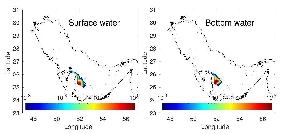
In a first example, the pollutant remained in the dissolved form, without adsorption in sediments (distribution coefficient set to zero). Finally, the five tidal constituents with their residuals were considered. A wind forecast was not used in this simulation. Results of this simulation are presented in Figure 4, where maps showing the calculated pollutant distributions in the surface and bottom water layers are shown. The pollutant was transported to the south, reaching a long extension of the coast. The distributions in the bottom water reflected that of the surface.
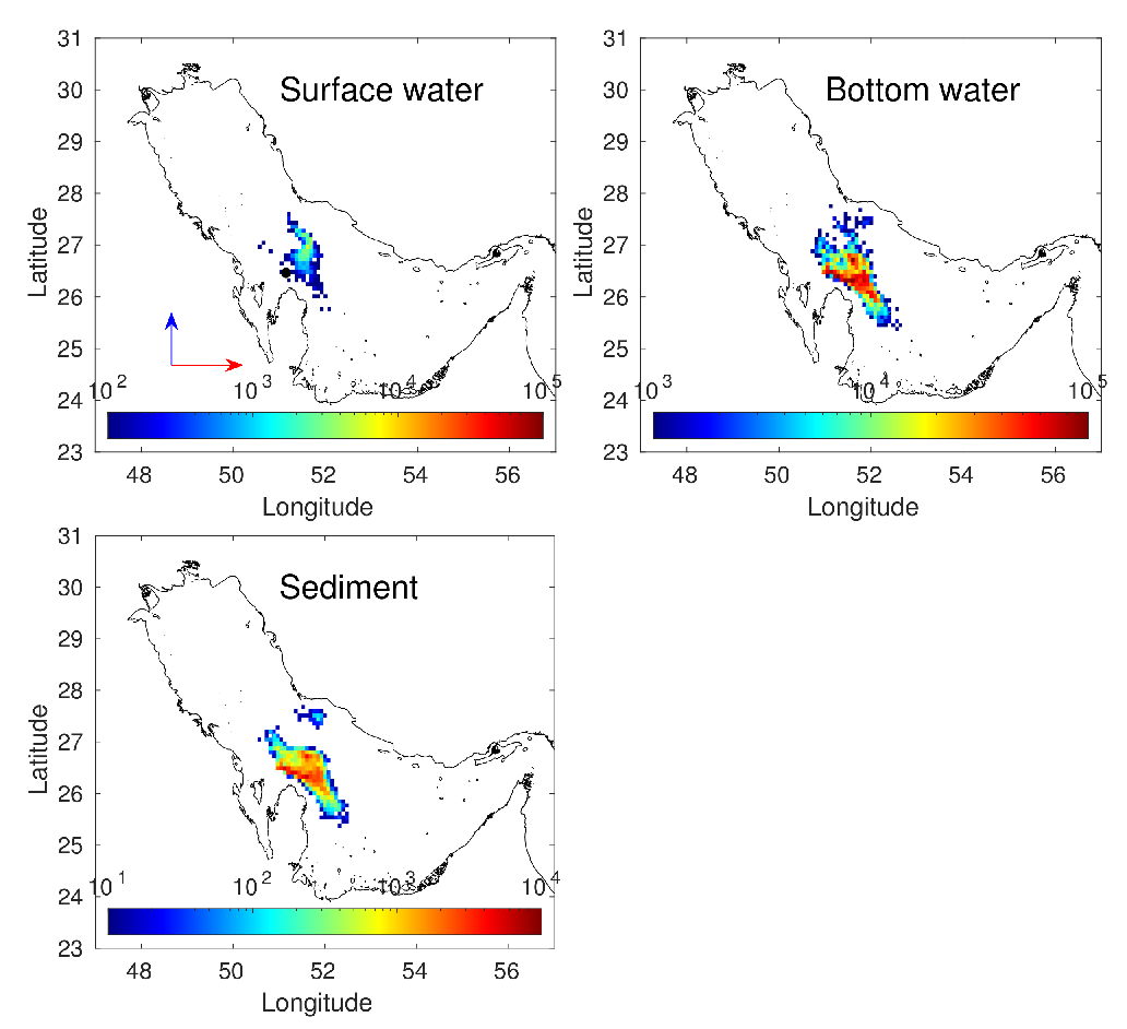
In a second experiment, exactly the same hypothetical accident was simulated, but it was supposed that the released contaminant was Hg, a toxic heavy metal whose distribution coefficient is equal to 30 m/kg [16]; thus, it presents a high affinity to be fixed to the sediments. The results of this simulation are presented in Figure 5, where a map showing the calculated concentrations in sediments (units/kg) is added. Due to the metal adsorption on the sediment, concentrations in the surface water are lower than in the case of the dissolved pollutant (note that the magnitude of the release is the same in both cases, as well as color scales in Figure 4 and Figure 5). In addition, pollutants with high affinity to the sediments are more immobile than those remaining in solution. This can be clearly seen by comparing the distributions in the bottom water layer: in the case of Hg, the peak concentrations remain in the area near the spill location.
A final numerical experiment was carried out to illustrate the effects of a local wind due to a local storm, for instance. The Hg simulation previously described was repeated, but it was considered that during the first 5 days, a 5 m/s was blowing from the west, which then increased speed to 20 m/s and changed direction to a northward wind. The results are presented in Figure 6. Obviously, the pollutant was initially transported to the central APG due to the west wind, and later, there was a significant transport to the north caused by the south wind. Actually, some Hg approached the eastern coast of the APG, and a spot of contaminated sediment was apparent there.
4. Conclusions
The transport model is easy to set up for any situation since it only requires the modification of a few input files specifying the pollutant properties (decay constant and distribution coefficient) and release characteristics (magnitude, location, date, time and duration). Running times are short (a few minutes for a several-day-long simulation), even on a desktop PC, which makes it appropriate for a rapid assessment of a hypothetical accident occurring in the APG. The model is based upon sound and solid mathematical and numerical approaches which have been widely validated before (see [4,14,18] for instance).
The geochemical behaviour of contaminants should be described within marine transport models, since the resulting concentrations depend on the affinity of the pollutant to be fixed to the sediment. This was clearly shown with the simulations carried out comparing the dissolved contaminant and with Hg.
Although the HYCOM model, used to obtain baroclinic circulation, already includes atmospheric forcing, a simple methodology to incorporate the effects of local weather events which could not be considered within the HYCOM, such as a sudden local storm, was described as well.
The present model only provides pollutant concentrations in abiotic compartments (surface and deep waters and sediments). Further research will incorporate a foodweb model which could describe the adsorption of such pollutants by fish. Advances in this topic are presented, for instance, in [23].
Funding
This research was partially funded by the Spanish Ministerio de Ciencia, Innovación y Universidades project PGC2018-094546-B-I00 and Junta de Andalucía (Consejería de Economía y Conocimiento) project US-1263369.
Institutional Review Board Statement
Not applicable.
Informed Consent Statement
Not applicable.
Data Availability Statement
Not applicable.
Conflicts of Interest
The authors declare no conflict of interest. The funders had no role in the design of the study.
Abbreviations
The following abbreviations are used in this manuscript:
| APG | Arabian/Persian Gulf |
| IAEA | International Atomic Energy Agency |
| HYCOM | Hybrid Coordinate Ocean Model |
References
- Iosjpe, M.; Brown, J.; Strand, P. Modified approach for box modelling of radiological consequences from releases into marine environment. J. Environ. Radioact. 2002, 60, 91–103. [Google Scholar] [CrossRef]
- Maderich, V.; Bezhenar, R.; Heling, R.; de With, G.; Jung, K.T.; Myoung, J.G.; Cho, Y.K.; Qiao, F.; Robertson, L. Regional long-term model of radioactivity dispersion and fate in the northwestern Pacific and adjacent seas: Application to the Fukushima Dai-ichi accident. J. Environ. Radioact. 2014, 131, 4–18. [Google Scholar] [CrossRef] [PubMed]
- Wu, Y.; Falconer, R.; Lin, B. Modelling trace metal concentration distributions in estuarine waters. Estuar. Coast. Shelf Sci. 2005, 64, 699–709. [Google Scholar] [CrossRef]
- Periáñez, R.; Casas-Ruíz, M.; Bolívar, J.P. Tidal circulation, sediment and pollutant transport in Cádiz Bay (SW Spain): A modelling study. Ocean Eng. 2013, 69, 60–69. [Google Scholar] [CrossRef]
- Elliott, A.J.; Wilkins, B.T.; Mansfield, P. On the disposal of contaminated milk in coastal waters. Mar. Pollut. Bull. 2001, 42, 927–934. [Google Scholar] [CrossRef]
- Havens, H.; Luther, M.E.; Meyers, S.D. A coastal prediction system as an event response tool: Particle tracking simulation of an anhydrous ammonia spill in Tampa Bay. Mar. Pol. Bull. 2009, 58, 1202–1209. [Google Scholar] [CrossRef] [PubMed]
- Kowalik, Z.; Murty, T.S. Numerical Modelling of Ocean Dynamics. World Scientific: Singapore, 1993. [Google Scholar]
- Periáñez, R.; Bezhenar, R.; Brovchenko, I.; Duffa, C.; Iosjpe, M.; Jung, K.T.; Kim, K.O.; Kobayashi, T.; Liptak, L.; Maderich, V.; et al. Marine radionuclide dispersion modelling: Recent developments, problems and challenges. Env. Mod. Soft. 2019, 122, 104523. [Google Scholar]
- Abdi, M.R.; Faghihian, H.; Kamali, M.; Mostajaboddavati, M.; Hasanzadeh, A. Distribution of natural radionuclides on coasts of Bushehr, Persian Gulf, Iran. Iran. J. Sci. Technol. Trans. A 2006, 30, 259–269. [Google Scholar]
- Al-Ghamdi, H.; Al-Muqrin, A.; El-Sharkawy, A. Assessment of natural radioactivity and 137 Cs in some coastal areas of the Saudi Arabian gulf. Mar. Pol. Bull. 2016, 104, 29–33. [Google Scholar] [CrossRef] [PubMed]
- Uddin, S.; Fowler, S.W.; Behbehani, M.; Al-Ghadban, A.N.; Swarzenski, P.W.; Al-Awadhi, N. A review of radioactivity in the Gulf region. Mar. Pol. Bull. 2020, 159, 111481. [Google Scholar] [CrossRef] [PubMed]
- Al-Rabeh, A.H.; Lardner, R.W.; Gunay, N. Gulfspill Version 2.0: A software package for oil spills in the Arabian Gulf. Environ. Mod. Soft. 2020, 15, 425–442. [Google Scholar] [CrossRef]
- Periáñez, R. A Lagrangian oil spill transport model for the Red Sea. Ocean Eng. 2020, 217, 107953. [Google Scholar] [CrossRef]
- Periáñez, R. Models for predicting the transport of radionuclides in the Red Sea. J. Environ. Radioact. 2020, 223–224, 106396. [Google Scholar] [CrossRef] [PubMed]
- Periáñez, R.; Elliott, A.J. A particle tracking method for simulating the dispersion of non conservative radionuclides in coastal waters. J. Environ. Radioact. 2002, 58, 13–33. [Google Scholar] [CrossRef]
- IAEA. Sediment Distribution Coefficients and Concentration Factors for Biota in the Marine Environment; Technical Reports Series 422; International Atomic Energy Agency: Vienna, Austria, 2004. [Google Scholar]
- Pugh, D.T. Tides, Surges and Mean Sea Level; Wiley: Chichester, UK, 1987; p. 472. [Google Scholar]
- Periáñez, R.; Pascual-Granged, A. Modelling surface radioactive, chemical and oil spills in the Strait of Gibraltar. Comp. Geosc. 2008, 34, 163–180. [Google Scholar] [CrossRef]
- Pous, S.; Carton, X.; Lazure, P. A process study of the tidal circulation in the Persian Gulf. Open J. Mar. Sci. 2012, 2, 131–140. [Google Scholar] [CrossRef] [Green Version]
- Parker, B.B. Tidal Analysis and Prediction; NOAA, NOS Center for Operational Oceanographic Products and Services: Silver Spring, MD, USA, 2007. [Google Scholar]
- Bleck, R. An oceanic general circulation model framed in hybrid isopycnic-Cartesian coordinates. Ocean Mod. 2001, 4, 55–88. [Google Scholar] [CrossRef]
- Yao, F.; Johns, W.E. A HYCOM modeling study of the Persian Gulf: 1. Model configurations and surface circulation. J. Geophys. Res. 2010, 115, C11017. [Google Scholar] [CrossRef] [Green Version]
- de With, G.; Bezhenar, R.; Maderich, V.; Yevdin, Y.; Iosjpe, M.; Jung, K.T.; Qiao, F.; Perianez, R. Development of a dynamic food chain model for assessment of the radiological impact from radioactive releases to the aquatic environment. J. Environ. Radioact. 2021, 233, 106615. [Google Scholar] [CrossRef] [PubMed]
Figure 1.
Map of the APG, which corresponds to the present model domain. Isobaths of 20, 40, 60, 80 and 100 m are drawn.
Figure 1.
Map of the APG, which corresponds to the present model domain. Isobaths of 20, 40, 60, 80 and 100 m are drawn.

Figure 2.
Comparison between calculated and observed amplitudes for the semidiurnal (left) and diurnal (right) constituents considered in the model.
Figure 2.
Comparison between calculated and observed amplitudes for the semidiurnal (left) and diurnal (right) constituents considered in the model.

Figure 3.
Files which should be edited for a given simulation.

Figure 4.
Calculated concentrations in the surface layer (units/m) and inventory (units/m) in the bottom water layer for the dissolved pollutant release after 30 days. The black dot in the surface water map indicates the release point.
Figure 4.
Calculated concentrations in the surface layer (units/m) and inventory (units/m) in the bottom water layer for the dissolved pollutant release after 30 days. The black dot in the surface water map indicates the release point.

Figure 5.
Calculated concentrations in the surface layer (units/m), inventory (units/m) in the bottom water layer and concentrations in sediments (units/kg) for the Hg release after 30 days. The black dot in the surface water map indicates the release point.
Figure 5.
Calculated concentrations in the surface layer (units/m), inventory (units/m) in the bottom water layer and concentrations in sediments (units/kg) for the Hg release after 30 days. The black dot in the surface water map indicates the release point.

Figure 6.
The same as Figure 5 but adding winds due to a local storm. See the main text for details. Arrows in the surface water map indicate the wind direction: west (red) and south (blue) winds.
Figure 6.
The same as Figure 5 but adding winds due to a local storm. See the main text for details. Arrows in the surface water map indicate the wind direction: west (red) and south (blue) winds.


Table 1.
Model availability.
| Program Name | APERTRACK |
|---|---|
| Developer | R. Periáñez, University of Sevilla |
| Contact | [email protected] |
| Hardware | Desktop PC |
| Program code | Fortran |
| Cost | Free |
| Availability | https://personal.us.es/rperianez/ (accessed on 15 November 2021) |
Table 2.
Input files which must be modified for each specific simulation. It is required to modify tide-data.dat only if a simulation for a year other than 2021 including tidal circulation is to be carried out.
Table 2.
Input files which must be modified for each specific simulation. It is required to modify tide-data.dat only if a simulation for a year other than 2021 including tidal circulation is to be carried out.
| tide-data.dat | Equilibrium arguments and nodal factors |
| release.dat | Release data and simulation time |
| RN.dat | Contaminant properties (decay constant and ) |
| input.dat | Switches to include or not tidal circulation |
| wind.dat | Local wind data |
Publisher’s Note: MDPI stays neutral with regard to jurisdictional claims in published maps and institutional affiliations. |
© 2021 by the author. Licensee MDPI, Basel, Switzerland. This article is an open access article distributed under the terms and conditions of the Creative Commons Attribution (CC BY) license (https://creativecommons.org/licenses/by/4.0/).
Share and Cite
MDPI and ACS Style
Periáñez, R. A Lagrangian Tool for Simulating the Transport of Chemical Pollutants in the Arabian/Persian Gulf. Modelling 2021, 2, 675-685. https://0-doi-org.brum.beds.ac.uk/10.3390/modelling2040036
AMA Style
Periáñez R. A Lagrangian Tool for Simulating the Transport of Chemical Pollutants in the Arabian/Persian Gulf. Modelling. 2021; 2(4):675-685. https://0-doi-org.brum.beds.ac.uk/10.3390/modelling2040036
Chicago/Turabian StylePeriáñez, Raúl. 2021. "A Lagrangian Tool for Simulating the Transport of Chemical Pollutants in the Arabian/Persian Gulf" Modelling 2, no. 4: 675-685. https://0-doi-org.brum.beds.ac.uk/10.3390/modelling2040036