1. Introduction
We live in a society that is marked by the rapid development of sciences and technologies [
1,
2]. Historically, technological advances have always played a significant role and signaled major changes for humanity [
3]. Recently, the advance of new technologies has been rapidly accelerating, resulting in the increased usage of robotics and embedded systems [
4,
5,
6,
7,
8,
9]. It is without doubt that everyone in the industry and private sector must adopt the new technologies, embrace the advances, and utilize the inter-connectivity and new optimization algorithms if they wish to be competitive in the new era; in other words, they should follow the new industrial evolution, expressed succinctly with the term Industry 4.0 [
10].
Warehouses and storage facilities are one application area in which robotics and embedded systems are prominent [
11,
12]. Warehouse and manufacturing environments have long been a potential arena for robotics and automation tasks to assist humans in producing better and faster results. Warehouses are one of the most important aspects of logistics since they are widely used for storing or buffering goods between two points of consumption. Receiving, moving, putting away, storing, order picking, cross-docking, and delivering are the basic warehouse operations. The time spent on each of these operations can be divided into the following sub-operations, according to Tompkins et al. [
13]: traveling (50 percent), searching (20 percent), choosing (15 percent), setup (10 percent), and other unforeseen circumstances (5 percent). As can be seen, travel consumes a significant amount of time, making it a prime candidate for optimization.
The goal of this study is to solve the delivery problem in warehouse environments for multiple heterogeneous robots, which are robots with varying capabilities, characteristics and features. Our proposed algorithm, in particular, is capable of solving the internal warehouse delivery problem with a team of diverged robots. The algorithm is also capable of finding the optimal location for power stations—locations in which the robots “rest”, meaning that they charge their batteries and wait for a new task to be allocated to them. Furthermore, each delivery task is allocated to the most suitable robot, increasing warehouse productivity and reducing delivery time. The path taken by each robot is determined by its technical requirements, which include type, speed, and maximum carrying weight. The algorithm’s key innovation is that it solves the warehouse internal distribution problem by using a team of several robots and taking into account the various requirements of each robot. We have created an automated simulation tool to visualize, analyze, and calculate the performance of our algorithm.
The rest of the manuscript is structured as follows:
Section 2 presents works found in the literature that are similar to ours. After that, the proposed algorithm is presented in
Section 3. The experimental results and the methodology that we used to evaluate our algorithm are presented in
Section 4. IoT and hardware acceleration techniques are discussed in
Section 5. The final thoughts and conclusions are given in
Section 6.
2. Related Work
The process of simultaneously planning appropriate paths for robots among various solutions can be defined as the routing problem. The reduction in travel costs is one of the aims of routing. Several algorithms have been proposed to solve the routing problem up to this stage, and they are divided into two categories: static [
14,
15] and dynamic [
16,
17]. Dynamic algorithms, in contrast to static routing, adapt to changes in the environment and the robot, resulting in increased efficiency. It is clear that, due to the high computational complexity of the routing process, several papers found in the literature do not take into account important features in the routing process, such as robots of various types, speeds, and dynamic robot positions. Because of this, verifying the proposed algorithm and benchmarking the simulation tool proved to be a difficult task; having no point of reference generates difficulties when evaluating new ideas.
In several research studies, the route is determined by considering the shortest path. Broadbent et al. [
18] introduced the idea of conflict-free and shortest-time robot routing for the first time. The presented methodology uses Dijkstra’s shortest path algorithm to produce a matrix that defines the vehicle path occupation time.
For the dynamic routing of robots in a bidirectional path network, Kim and Tanchoco [
19] combined Dijkstra’s algorithm with the idea of a time windows graph. They proposed formulas to account for time curves, but their findings do not reflect this.
To the approach proposed by Kim and Tanchoco, Maza and Castagna [
20,
21] introduced a layer of real-time control. They introduced a robust predictive method of routing without conflicts in [
20], and they developed two algorithms to monitor the robots’ mechanism, using a predictive method when the system is subject to threats and contingencies in real time, preventing conflicts [
21]. Both implementations fail to account for the differences in robot characteristics.
The research work presented in this paper is an extension of our previous conference paper [
22] and is different from the aforementioned works in three main aspects: (1) we give a solution to the task allocation issue inside modern warehouses, where the environment is dynamically changing, meaning that the location of each robot changes; (2) the algorithm performs an in-depth task analysis, meaning that it calculates the task route as well as the energy cost; finally, (3) in order to evaluate the performance and capabilities of the proposed methodology, we developed a synthetic environment benchmarking tool that is capable of calculating realistic warehouse environments.
3. The Proposed Algorithm
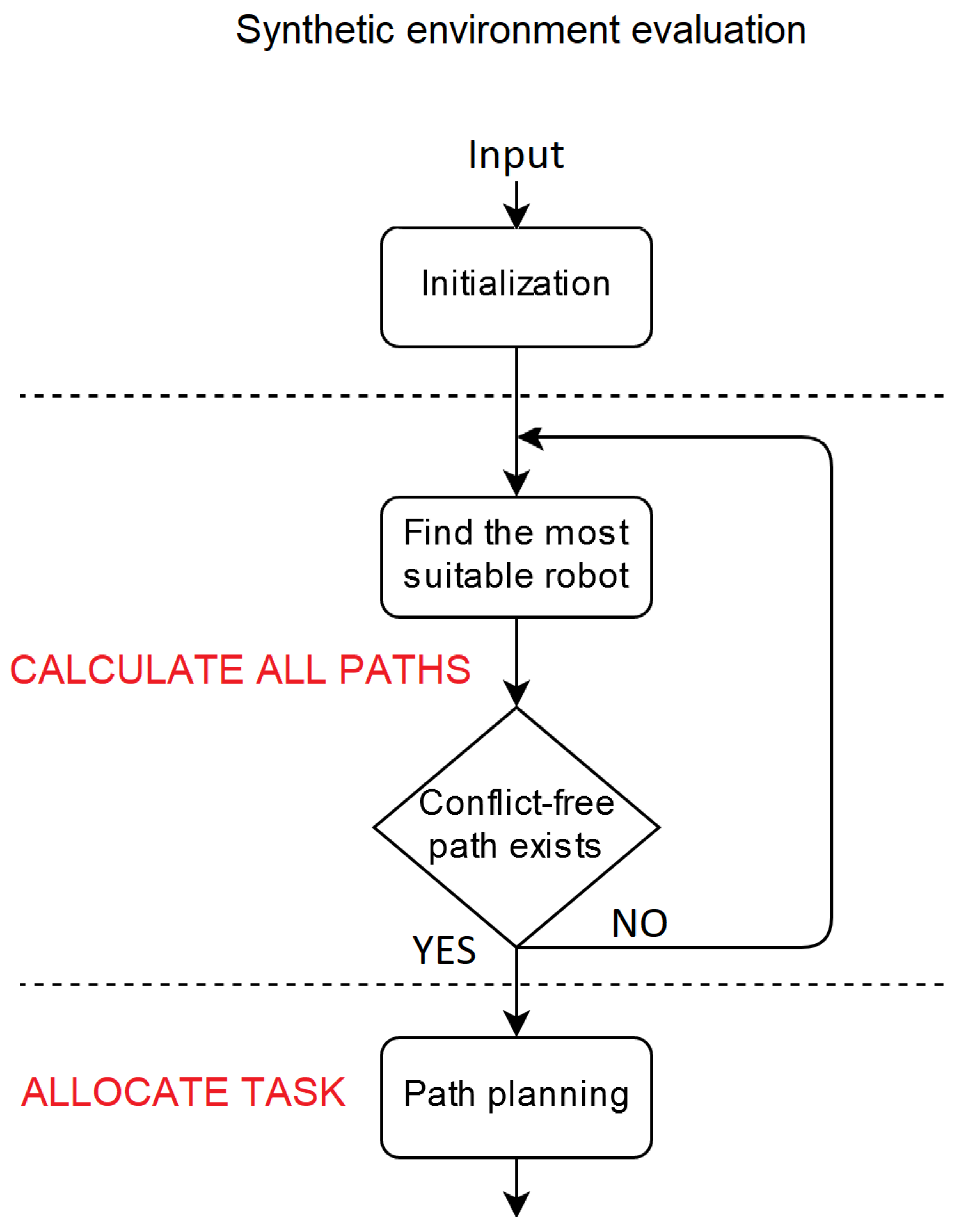
There are three key stages in the proposed algorithm (
Figure 1). The algorithm’s initialization is the first stage. The size and topology of the environment, obstacle locations, robot specifications (such as form, speed, and positions), and current in-progress tasks are all inputs to the algorithm. The current delivery role is processed in the second stage. During this stage, the state of all robots is assessed, and the most appropriate robot is chosen. This stage’s output is a descending list of all robots ranked according to their suitability for the mission. Robots whose current position is close to the product’s storage shelf are ranked higher on the list, while robots whose current location is far away are ranked lower. The list excludes robots whose maximum carrying weight is less than the product’s weight. The route for the selected robot is determined in the third stage. In order to prevent congestion and have a route that is free of conflicts, the algorithm considers the paths of other vehicles. We should note here that the passageway between the shelves might be too narrow for two or more robots to pass through. At any given time, only one robot can be found on a tile. If no path exists that is free of conflicts with other robots, the algorithm will repeat the procedure with the next most appropriate robot until one does. The algorithm terminates and outputs the route once a robot capable of completing the distribution task is found.
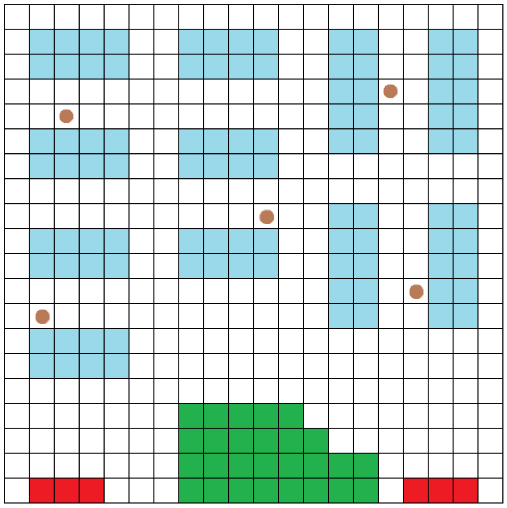
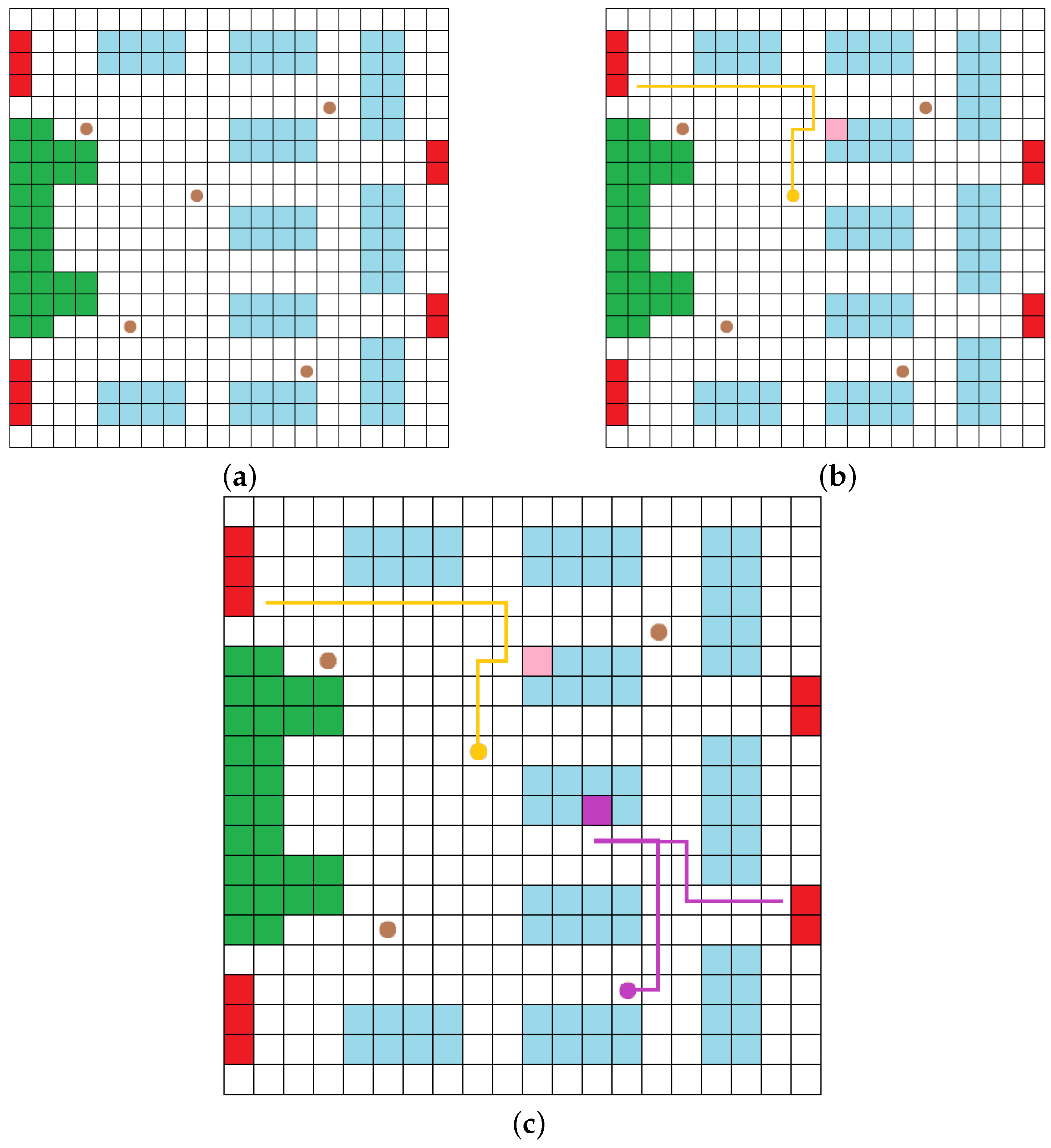
The environment, robots, and their respective requirements, as well as ongoing tasks, are all initialized in the first stage. Multiple tiles make up the environment, which is a two-dimensional Euclidean space. A (X, Y) coordinate is assigned to each tile. A tile is the smallest space that any robot can occupy, and each tile is equal to the next. Obstacles, shelves, and empty area are all examples of tiles that robots can navigate (
Figure 2). Obstacles are places that robots cannot traverse by themselves. Shelves are used to store products. Each product’s position is determined by its row, column, and shelf height. At least one Place of Delivery (PoD) exists in each warehouse, where the requested product must be delivered.
Form, speed, maximum load weight, and energy consumption are all characteristics of robots. All robots can handle items that are stored on the ground floor. Some robots, on the other hand, can reach higher heights and reach items placed on higher shelves. The speed at which robots travel is another distinguishing feature. The robot’s movement speed is measured in tiles per unit of time and is defined as the rate at which it can move from one tile to another. Robot A, for example, could have twice the speed of Robot B, implying that Robot A can travel twice the distance in the same amount of time as Robot B. The overall load weight of robots is another characteristic. Only light-weight items can be carried by robots; robots can only hold objects that are lighter than the robot’s full load weight. Another characteristic of robots is their energy usage. The energy usage of each robot when traveling in a straight line and when doing a 90° turn are also taken into account.
The distribution task is processed in the second stage. The algorithm calculates the total distance required to deliver the requested product to the PoD for each idle robot capable of carrying it. A Dijkstra implementation is used to find the shortest distance between each robot [
23]. The total distance covered,
, for each robot is the sum of the distance from its current position to the product location,
, and the distance from the product location to the PoD
(Equation (
1)).
After the distance is calculated, for each potential robot, the algorithm calculates the total energy required to complete the delivery task. The total energy
is calculated using Equation (
2).
where
represents the total distance traveled in a straight line,
represents the robot’s energy consumption when traveling in a straight line,
represents the number of 90 degree turns, and
represents the robot’s energy consumption for a 90 degree turn. Robots usually have different energy consumption when they move in a straight line, and when they make 90 degree turns. Depending on the size of the robot and its type, these numbers can be very different. The exact reason why this happens is out of the scope of this paper but briefly, this happens because of the energy cost of building momentum and the energy cost of moving while stationary. The energy used to pick up the product from the shelf is considered insignificant and is therefore ignored. In the future, if the algorithm is used in locations with shelves of tens of rows, we intend to implement a feature that takes into account this minor but important energy consumption.
Finally, for each potential robot, the algorithm calculates the total time required to complete the delivery task. The total time
is calculated using Equation (
3).
where
is the required time for the robot to travel from its current position to the position of the product and
is the required time for the robot to travel from the product location to the PoD.
As different robots have different straight-line and turning speeds, the general time calculation is based on Equation (
4).
where
is the total distance traveled in a straight path,
is the speed of the robot while moving forward,
is the total number of turns, and
is the time required for the robot to perform a 90° turn.
Following the completion of the total energy and time needed for each possible robot to complete the delivery task, the algorithm measures each robot’s performance. The energy cost per time unit is used to measure performance. In other words, robots that consume a lot of energy in relation to the processing time are penalized, while robots that provide a lot of energy per time unit are rewarded (Equation (
5)).
where
is the efficiency of the each robot,
is the total energy consumption, and
is the total time required to complete the delivery task. The results are stored in an array in descending order of efficiency.
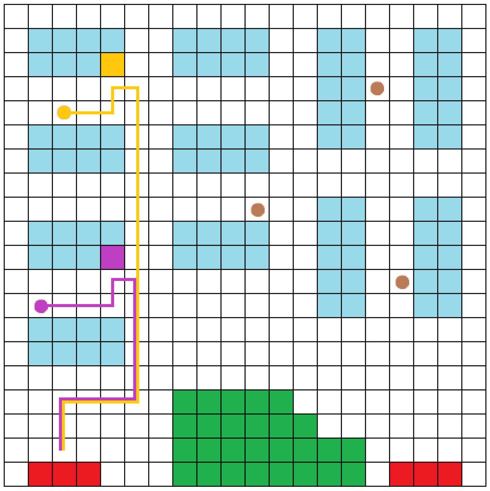
The first robot on the efficiency array is chosen in the third stage. The route calculated using Dijkstra’s algorithm in the previous stage is checked for collisions. The algorithm calculates the time at which each tile will be traversed by a robot based on the movement capabilities of the respective robot for the measured path and for any path of an active delivery task. If two or more robots are traversing a tile at the same time, the determined path is discarded, and the next most effective robot is examined. This process is repeated until a direction is identified that is free of conflict. The active delivery tasks are updated with the final calculated route, and the delivery process begins (
Figure 3). Using this method, the most powerful robot capable of delivering the product without causing any conflicts is always chosen.
4. Experiments and Results
4.1. Synthetic Benchmarks
In order to evaluate the proposed algorithm, find the optimal robot paths for the warehouse delivery tasks and calculate the optimal power stations, we needed to develop a tool that would generate realistic environments. This need was reinforced by the fact that actual warehouse data sets do not exist yet. Big companies and robotized warehouse operators do not openly share these data; therefore, in order to evaluate warehouse management algorithms, developing a new tool was necessary. The tool that we built for the synthetic benchmarks generates realistic maps of warehouses, including products and robots. The warehouse maps that are generated include the pseudo-random placement of the robots, the products and other warehouse parameters. Then, it pseudo-randomly generates tasks that are then fed to the algorithm. By using this tool, we can perform thousands of simulations in few hours. The generator utilizes our knowledge on e-shops warehouses, general knowledge about e-commerce, fruitful discussions with local shop owners and articles on subject matter expert journals, such as the
International Journal of Production Research. The actual simulation execution time is dependent on multiple factors, including the size of the warehouse, the number and types of robots, the number of products and the number of allocation tasks. The simulator enables real-time communication with the optimal path algorithm. We used the Transmission Control Protocol (TCP) socket in a predefined port, which has the ability to display the movements of the robots in real time. When starting the simulator, all the information, including the positions of the obstacles and the grid dimensions, are entered in the JSON format [
24]. By executing the optimal path algorithm and finding the path, the
x,
y points are sent to the simulator, which plots the path of each robot. The simulator accepts a JSON input in which the demands of the algorithm are recorded: The number of the tiles of the
x-axis and the
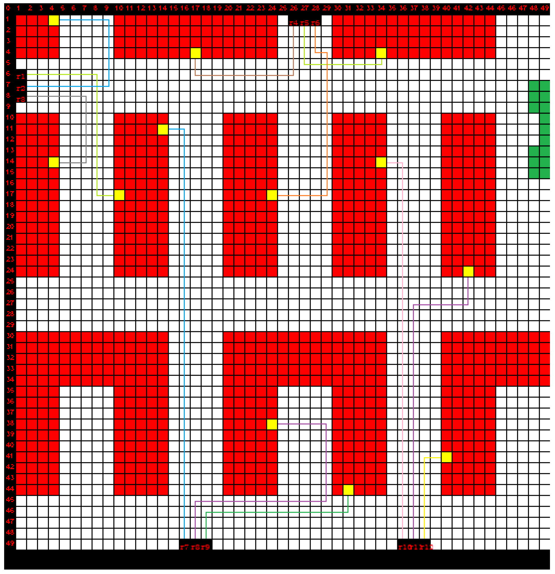
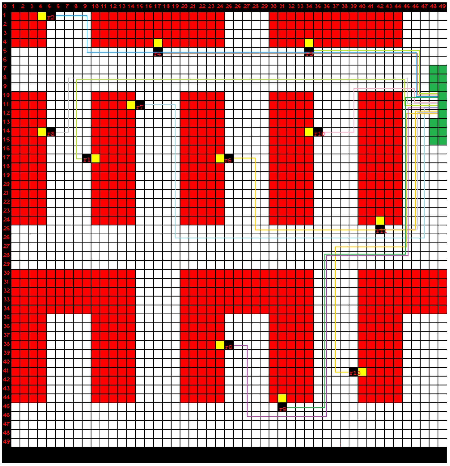
y-axis. The obstacles are divided into groups. Each group includes the color illustration and obstacle positions in the simulation area. The robots that calculate the optimal route take into consideration the groups of the obstacles that they belong to (obstacles that cannot be overcome, for example, low and high obstacles). Next, the JSON file includes the number of robots, their name, and starting point. The initial position of the robots in the simulator is indicated by a black square. The movements of the robots, extracted from the algorithm, include the name of the robot and the color of the lines that appear during the simulation for each one. After running the simulator, a text file that includes the simulator run time, the number of robots, the total number of the tiles and the movements that were being displayed on the simulator is extracted. In addition, a grid image is extracted depicting the movements of the robots and the obstacles.
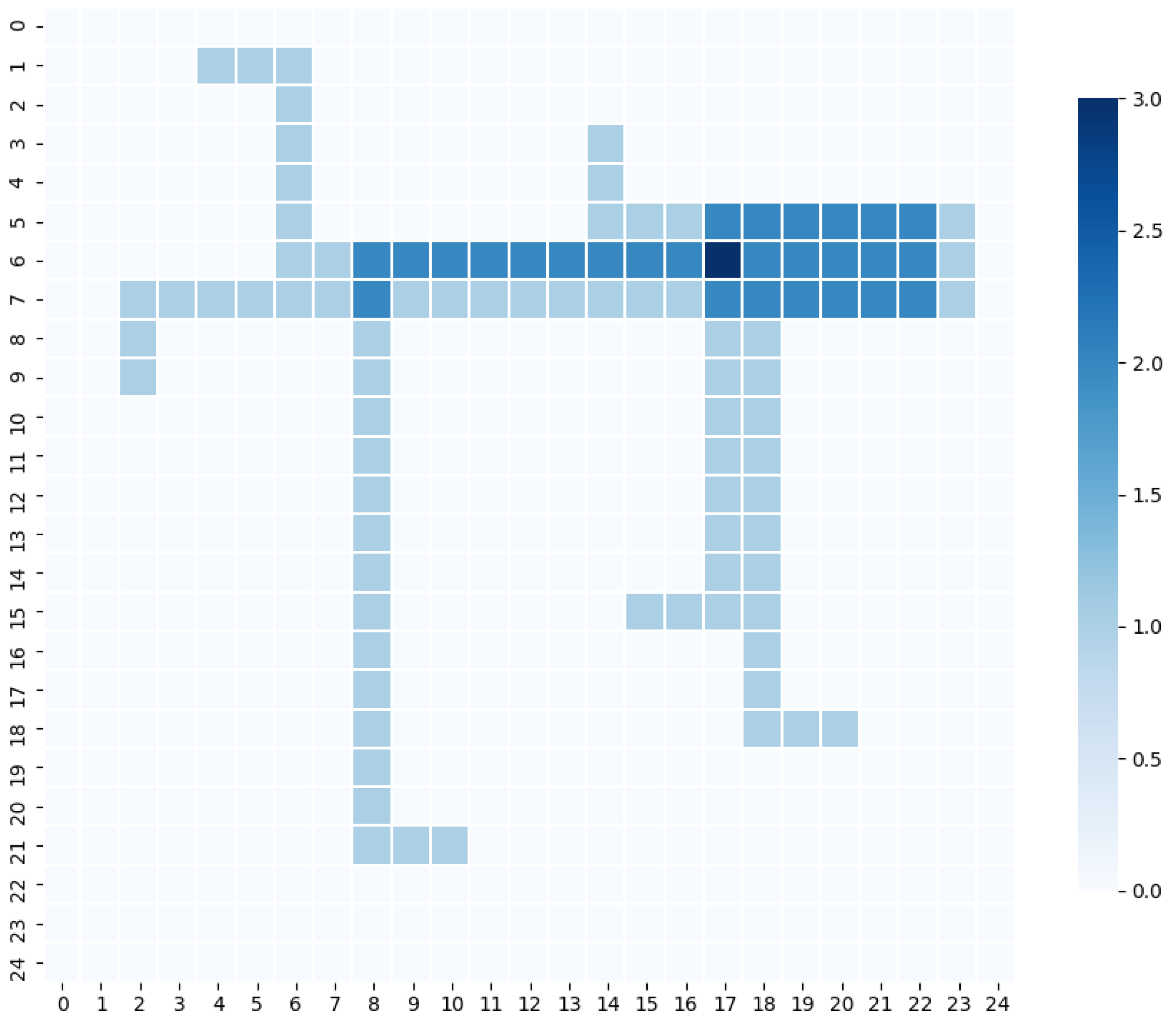
Finally, our simulation tool can graphically represent the environment, the paths of the robots and the heat map (
Figure 4) of the environment.
Figure 5 presents an example of the initialization of the environment and
Figure 6 presents the initialization of the robots. The heat map shows the magnitude of a phenomenon as color in two dimensions. In our case, it uses color-coded visualization to illustrate the paths or corridors that are traversed by multiple robots; the more popular routes carry a darker tone. This visualization could help the warehouse manager to re-organize the placement of products to avoid route saturation and over-usage. This way, by having a visual representation of the actual warehouse and all the other important data, the interpretation of the results of our algorithm is much easier and human friendly.
4.2. Simulation Results
The proposed algorithm is classified as an offline algorithm, which means that it already has knowledge of the factory, robot positions and characteristics, and product locations. The development of an automated simulation tool was needed in order to test our algorithm and perform multiple experiments. We created a tool in Python that takes basic user inputs, such as warehouse size, robot position, robot type, product count, and percentage of unoccupied tiles, and generates a JSON file that describes the generated warehouse environment.
This tool can create warehouse environments with items that are randomly placed. The created file is then used as input for our proposed algorithm, which automates the simulation process. The proposed algorithm was tested in a [
] =
. 70% simulated warehouse environment. Shelves with items, obstacles, and office facilities took up 70 percent of the tiles. To mimic realistic warehouse designs, the shelves were arranged in rows. The robot’s initial positions in the warehouse were all over the place. We used an Intel Core i7 3770K CPU with 16 GB of RAM for this simulation. The simulation results are shown in
Table 1.
Figure 7 presents the algorithm results for a 20 × 20 environment, with 5 robots and multiple exits.
It is worth noting that, since no other research works have attempted to solve the problem addressed in this paper, a comparison of our findings is not possible. The topology of the warehouse, the location of shelves, and the initial locations of the robots do not appear to influence the algorithm’s execution time in our tests. The time it takes the algorithm to find a solution for each distribution task is strongly influenced by the environment’s dimensions and the number of robots.
The simulation results indicate that the scaling of the algorithm is almost linear. However, this depends on the environment dimensions, number of robots, simultaneous tasks and other factors. In extreme cases, with very large environments (with dimensions of 10,000 × 10,000, for example), the algorithm does seem to slow down. However, these extreme cases are unrealistic and are out of the scope of this research.
5. IoT and Hardware Acceleration
Finding the paths of the robots and the locations of power stations using the proposed system requires a significant amount of computational power. There are ways, however, that we can improve the proposed model by further increasing its efficiency and decreasing the computation time. By doing this, the proposed algorithm could be executed on site by IoT devices and possibly the robotic vehicles themselves.
A potential solution for improving the proposed system’s execution speed and efficiency is to accelerate the navigation algorithm on an FPGA board, such as the Zynq-7000 ARM/FPGA SoC. Over the last few decades, FPGA boards have become increasingly popular. FPGA software has a number of benefits over software running on a CPU or GPU, including faster execution and lower power consumption. The FPGA board, as well as a high-performance conventional server, could be housed in the cloud in the proposed framework. The server could offload the navigation process to the FPGA boards since it would obtain task details from the embedded systems in warehouses. PCIe networking is supported by a large number of boards, with a maximum theoretical bandwidth of 15.75 GB/s in version 3.0. However, the key drawback of FPGA boards is the higher technical cost and complexity. Custom hardware circuits are designed as part of the FPGA development phase. Traditionally, hardware circuits have been defined using Hardware Description Languages (HDL), such as VHDL and Verilog, and software has been programmed using a variety of programming languages, including Java, C, and Python. High Level Synthesis is an upcoming trend on FPGA (HLS). HLS enables standard programming languages, such as OpenCL or C++, to be used to program FPGAs, allowing for a much higher degree of abstraction. Programming FPGAs is still an order of magnitude more complex than programming instruction-based systems, even when using high-level languages. FPGA boards are only useful for speeding up the classification process at larger scales, where the system’s output advantage outweighs the increased complexity and engineering expense.
6. Conclusions
The usage of robotics in warehouses is constantly increasing, mainly because as technology advances, it becomes less expensive. The typical modern warehouse now includes autonomous robots that take over the allocated deliveries. This results in faster deliveries of the product, and increases the productivity of the warehouse. These autonomous robots, however, bring the problem of dynamic routing to the surface. Many researchers have attempted to propose a solution to this problem; the majority, however, do not take into account the different specifications of the warehouse robots in operation. These specifications include the power requirements, type of robot, energy cost of movement and more. This research paper proposes an algorithm that is capable of orchestrating a team of multiple warehouse robots, taking into account all the peculiarities of the robots in order to solve the task allocation problem of modern warehouses. Since data from large modern warehouses are not publicly available, in order to evaluate the algorithm, it was necessary to build an automatic synthetic benchmarking tool that generates realistic environments. Using this tool, we evaluated the effectiveness and stability of our algorithm. To the best of our knowledge, similar tools such as that presented in this paper are not found in the literature; therefore, we could not provide a comparison of the experiments in order to evaluate the effectiveness and the novelty of our tool. The work presented in this paper can be improved in the future by adding support for more complicated environments, with multiple floors, obstacles and parameters. Enhancements regarding the speed of the algorithm could also be made by utilizing hardware accelerators on the cloud and using Software As A Service (SaaS) techniques.


