
Application of Task-Aligned Model Based on Defect Detection


1
Department of Industrial Engineering and Management, National Taipei University of Technology, Taipei 10608, Taiwan
2
Department of Enterprise Solutions, Enterprise Business Group, Chunghwa Telecom Co., Ltd., Taipei 10048, Taiwan
*
Author to whom correspondence should be addressed.
Automation 2023, 4(4), 327-344; https://doi.org/10.3390/automation4040019
Submission received: 3 September 2023
/
Revised: 15 October 2023
/
Accepted: 24 October 2023
/
Published: 27 October 2023
(This article belongs to the Topic Smart Manufacturing and Industry 5.0)
Abstract
:In recent years, with the rise of the automation wave, reducing manual judgment, especially in defect detection in factories, has become crucial. The automation of image recognition has emerged as a significant challenge. However, the problem of how to effectively improve the classification of defect detection and the accuracy of the mean average precision (mAP) is a continuous process of improvement and has evolved from the original visual inspection of defects to the present deep learning detection system. This paper presents an application of deep learning, and the task-aligned approach is firstly used on metal defects, and the anchor and bounding box of objects and categories are continuously optimized by mutual correction. We used the task-aligned one-stage object detection (TOOD) model, then improved and optimized it, followed by deformable ConvNets v2 (DCNv2) to adjust the deformable convolution, and finally used soft efficient non-maximum suppression (Soft-NMS) to optimize intersection over union (IoU) and adjust the IoU threshold and many other experiments. In the Northeastern University surface defect detection dataset (NEU-DET) for surface defect detection, mAP increased from 75.4% to 77.9%, a 2.5% increase in mAP, and mAP was also improved compared to existing advanced models, which has potential for future use.
1. Introduction
The need for surface defect detection is present mostly in industrial production processes, as defects can occur in all kinds of industrial production processes. Possible causes include low quality raw materials, the low technical capacity to produce, or abnormal equipment, all of which can lead to defects in surface appearance.
However, in the past, defective objects produced in the factory production process were mostly eliminated by the eyes of many production line personnel one by one. In the mass production operation of the factory, the overall economic efficiency of production is usually handled by random inspection. This situation still causes customer dissatisfaction with defects, but there is no better way to optimize the existing production model.
As discussed in this paper, metal defects face more problems with human inspection; because the steel in the color display is a bright gray color, personnel need to spend more time and effort looking for defects compared with other general production factories. Furthermore, there are still patterns on the steel, so there will still be misjudgments under long-term human visual inspection, and the edges of the steel are also quite sharp, causing a lot of security risks to steel inspection.
Improvement in defect detection has become an important goal for all factories. With the advancement of technology, the use of camera images for steel defect detection can effectively negate the possible danger of the human approach. The contactless method of detecting defects and sending alarms increases safety by eliminating human contact. In addition, speed is also improved; the current hardware has very high computing performance, and faster computing can identify a large number of steel surface defects at the same time.
For example, on the NEU-DET dataset of common metal defects [1] (shown in Figure 1), the mAP of the current neural network model can reach about 70% and can identify many different types of defects, which can effectively enhance the speed, safety, and mAP of defect detection.
In addition, the history of image defect detection is classified into traditional image detection and deep learning detection. Traditional image detection uses CPU resources and can only classify simple images, with the development of classification systems such as support vector machine (SVM) [2], Random Forest [3], principal component analysis (PCA) [4], and k nearest neighbors (KNN) [5]. Later, in the rapid development of neural network architectures for deep learning-based detection [6,7,8,9,10,11,12], Ref. [6] introduced the real-time detection network (RDN) architecture to enhance mAP but with the drawback of higher computational requirements. Ref. [7] proposed the defect detection network (DDN) architecture, capable of generating more feature information, but it performs poorly on multiple scattered defects. Ref. [8] improved RetinaNet to construct the DEA_RetinaNet architecture, but there is still room for optimization when it comes to detecting scratches, crazing, and rolled-in scale defects. Ref. [9] introduced the channel attention and bidirectional feature fusion on a fully convolutional one-stage (CABF-FCOS) network architecture, which improved performance but came with a larger number of parameters, making it challenging to deploy on smaller devices. Ref. [10] presented the Improved-YOLOv5 network architecture, optimizing the original YOLOv5 structure, but occasional misclassification of defect categories still occurred. Ref. [11] proposed an end-to-end defect detection and classification network based on the single shot multiBox detector (SSD) architecture, but the accuracy remained relatively low. Ref. [12] introduced the DAssd-Net network architecture, which has only a small number of parameters, making it advantageous for deployment on small devices, and which performs well in detecting small metal defect objects.
The papers [6,7,8,9,10,11,12] use GPU resources to effectively recognize complex graphics so that mAP can be improved compared to traditional image detection and can be used in general factory production processes. Other than for metal defect detection, it has been applied to rail track surfaces [13,14,15,16], solar panels [17], and buildings [18] for defect detection.
Since the publication of AlexNet [19] in 2012, neural networks have grown rapidly, object detection using deep learning has achieved remarkable success, and many studies have been proposed with advanced techniques. Technically, there are two types of object detection: one-stage and two-stage object detection.
When object detection of the region proposal image and classification are processed at one time, it is called one-stage object detection. The first model adopted for one-stage object detection was OverFeat [20]. However, you only look once (YOLO) [21] is the most popular one. Further development of the SSD [22] allowed extraction of feature maps of different sizes and the use of region proposals of different sizes for classification.
When object detection is used to detect the region proposal image and then classify the objects in these regions, it is called two-stage object detection. R-CNN [23] was the first to use a selective search to detect more than 2000 region proposals and input them into CNN for classification in two-stage object detection. To improve the detection speed, Fast R-CNN [24] first convolved the entire image. The faster R-CNN [25] proposed that the region proposal network (RPN) could improve the speed. Cascade R-CNN [26] was further improved to achieve a more accurate prediction of object location by continuously increasing the IoU threshold between input and output, which in turn improved mAP.
To solve the lower mAP caused by various objects of different sizes in the image, an effective feature pyramid network (FPN) was proposed in previous studies [27]. Furthermore, RetinaNet [28] uses focal loss to solve the problem that too many negative sample objects that are easy to learn lead to large differences in positive and negative sample weights during training, resulting in a failure to improve easy learning, so that the mAP can be further improved.
In summarizing the above, the one-stage is higher in speed than the two-stage but lower in mAP than the two-stage. However, with the continuous development of hardware performance and neural network architecture, the accuracy and speed of object detection have been improved, and now there is no difference between one-stage and two-stage object detection, and both can be used for defect detection.
In the current neural network object detection model, the position of the bounding box in the image is precisely defined as the anchor, and there are two types of anchors: Anchor-based and Anchor-free. Anchor-based is designed with predefined boxes and number of boxes and is constantly learning through the neural network to correct for the best anchor and bounding box. The Anchor-based approach is used in algorithms such as Fast-RCNN [24], Faster-RCNN [25], and SSD [22]. Another Anchor-free algorithm is to directly predict an anchor point and a bounding box and then continuously learn to correct the optimal anchor and bounding box through neural networks. CenterNet [29], FCOS [30], and other algorithms use the Anchor-free approach.
Anchor-based calculation of IoU in the training step consumes a lot of GPU memory and training time, but, compared to Anchor-free, it can effectively handle object detection of different sizes in the image. However, with the development of FPN, the size object problem can also be solved effectively. In addition, Anchor-free tends to generate more negative samples during training, which is later solved effectively by the focal loss tuning algorithm.
Further, the adaptive training sample selection (ATSS) [31] was developed, and the reason for the large difference in mAP between Anchor-based and Anchor-free is due to the different definitions of positive and negative samples. ATSS optimization can be used to completely close the mAP discrepancy between Anchor-based and Anchor-free, which also opens up a new architectural framework.
As mentioned above, two different combinations of Anchor-based or Anchor-free are added to one-stage or two-stage object detection, resulting in a complete algorithm. In both Anchor-based and Anchor-free environments, the target object and the target classification are slightly different in terms of the optimal anchor and bounding box, resulting in a poorer prediction of the mAP. In particular, it is more difficult to learn about defective images on metal than on normal objects, resulting in a larger mAP difference.
The primary contributions of this work are given below.
- The first TOOD algorithm is applied for the detection of metal defects [32].
- In the NEU-DET metal defect dataset, the mAP is increased from 75.4% to 77.9%, an improvement of 2.5%, and the mAP is also improved compared with the existing model.
2. Related Work
2.1. Class and Location Independent Problem
In general object detection, class and location are processed together in two independent branches without any correlation between them. This may lead to a situation where the class score is high (correctly classified) but the status of the anchor and bounding box in the location may be different from the real object. On the contrary, the anchor and bounding box of the location are accurate, but the class score is low, leading to the incorrect identification of the object.
The TOOD algorithm [32] is a good solution to this problem using a task-aligned approach. The task-aligned head (T-head) classifies and locates the objects using task-aligned loss to calculate the loss and continuously adjusts to reduce the loss. The final optimization result is sent to task alignment learning (TAL), which sends the best result to finally improve mAP.
2.2. Complexity of Metal Defective Images
From Figure 1, we can see that the features of metal defect images are more complex and difficult to train than the features of general object detection, such as cars, motorcycles, people, cats, dogs, and so on. Deformable ConvNets (DCN) can effectively solve the problem of complex feature learning difficulties.
DCN [35] offsets the learned sampling points, and the offsets can expand the features in the learned image and calculate a new feature map based on the offsets. The feature map is a branch added to the general convolution to accomplish the above work, which does not affect the original general convolution operation but can effectively enhance the learning of complex object features.
The features are difficult to train, and DCNv2 [34] is used as the deformable convolution. Compared to DCN, it can be modulated on different spatial locations/bins in addition to offsets, and the concept of weights is added. By adjusting the effective feature learning with different offset weights and adjusting on different convolutional layers (conv3, conv4, conv5), mAP enhancement is achieved.
2.3. Optimize the Method of Selecting the Best Bounding Box
Non-maximum suppression (NMS) [36] often uses the method for the object bounding box in object detection. After the CNN model has determined the bounding boxes and calculated the probability scores of the objects, the NMS ranks the probability scores of the proposal bounding box from highest to lowest. Then the highest scoring proposal bounding box is selected to serve as the bounding box, and the others are deleted if they are overlapping with the suggested one. The remaining proposal bounding boxes will continue to be selected by the above process until there are no more proposal bounding boxes at the end. When the proposal bounding boxes of two objects are too close, the lower score box is removed, because the overlapping area is too large and it will cause a decrease in mAP.
Due to the disadvantages of NMS, this experiment uses Soft-NMS [33], which replaces the original deletion with a slightly lower score, so it can be continuously selected by comparison. Therefore, it can effectively improve mAP.
3. Methodology and Design
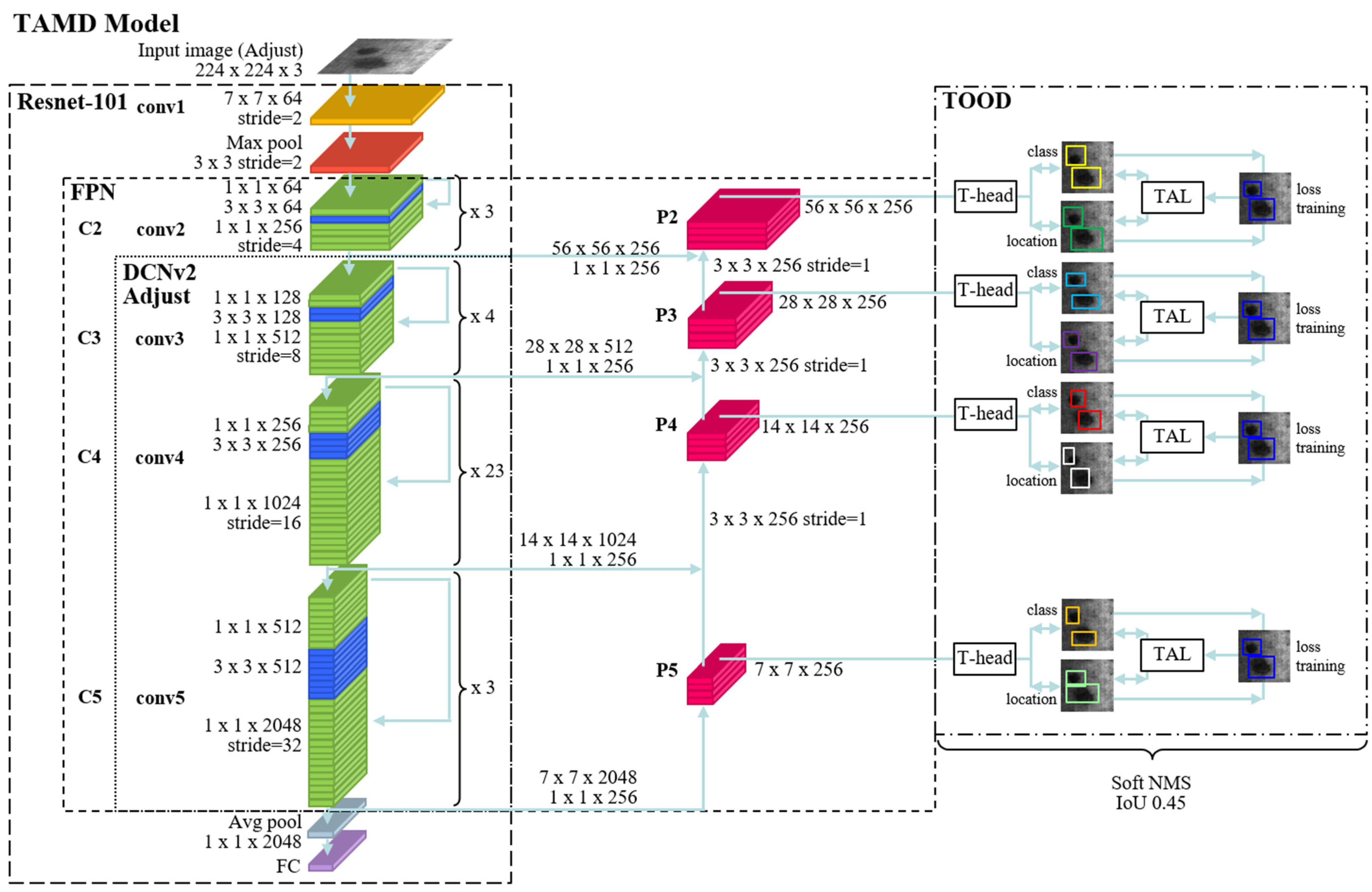
The system architecture of this study in Figure 2 and the technologies and functions are described below.
3.1. Baseline Convolution Architecture
In general, it is known that a pre-trained model in the COCO dataset [37], with pre-training weight, can decrease the training time and overfitting. The pre-trained model is then adjusted on the NEU-DET dataset, which usually has a better mAP and can effectively obtain the features from the metal defect images.
In this paper, various backbone networks have been tested, including ResNet-50/101 [38], or the more advanced ResNeXt-101 [39]. From the subsequent experiments, it was found that the use of ResNet has the following points.
- Comparison with CNN: ResNet can achieve high mAP with very few parameters, significantly reduce training time, and effectively reduce the occurrence of overfitting.
- Findings in the course of experiments: Under the same performance, the batch size can be larger than that of ResNeXt-101, but the mAP trained by ResNet-50/101 is much better than that of ResNeXt-101.
3.2. FPN
In metal defect images, different sizes of defective objects are often found. Feature acquisition on a single scale is usually not effective. Therefore, FPN is used to improve the C3-C5 layers (bottom-up) of the original ResNet. A skip connection is added, and the skip connection is designed to contain the feature map of the deepest layer (P5), and the top-down sampling is added correspondingly as shown in Figure 2. Finally, the inverse convolution structure grows from layer P5 to layer P2, and the feature map of the deepest layer of P5 can be added element-wise by gradually enlarging the size.
Although the depth of the P5-P4 layer in the FPN has already obtained higher resolution features [27], the corresponding features are easier to recognize, and thus the localization can be more precise. However, in the lower layers of P3-P2, the feature information is not significant, and the corresponding features become relatively inaccurate in localization. The TOOD algorithm provides classification and localization of proposal bounding boxes with more than one feature layer. The mAP can be enhanced by the classification and localization of the proposal bounding box on multiple layers with multiple fused features at different scales.
3.3. DCNv2
In a general neural network, the convolutional equation is shown in (1). R is defined as the size and dilation corresponding to the feature map x of the neural network. The weight of the parameter is denoted by w. The final export features map y.
In DCN, the learning sampling points are offsets. The offset is ΔPn. The modified convolution equation is shown in (2) [35].
In DCNv2, the DCN is optimized by offsetting the learning sampling points by ΔPn. Furthermore, the scalar weights Δmk for each learning sampling feature are modulated mechanisms. The modulation mechanism can be performed in different spatial locations/bins, as shown in (3) [34] below.
Combining the experiments of [34] should be effective in improving mAP in various other algorithms. However, the overall training computation is increased due to the increase in weight Δmk.
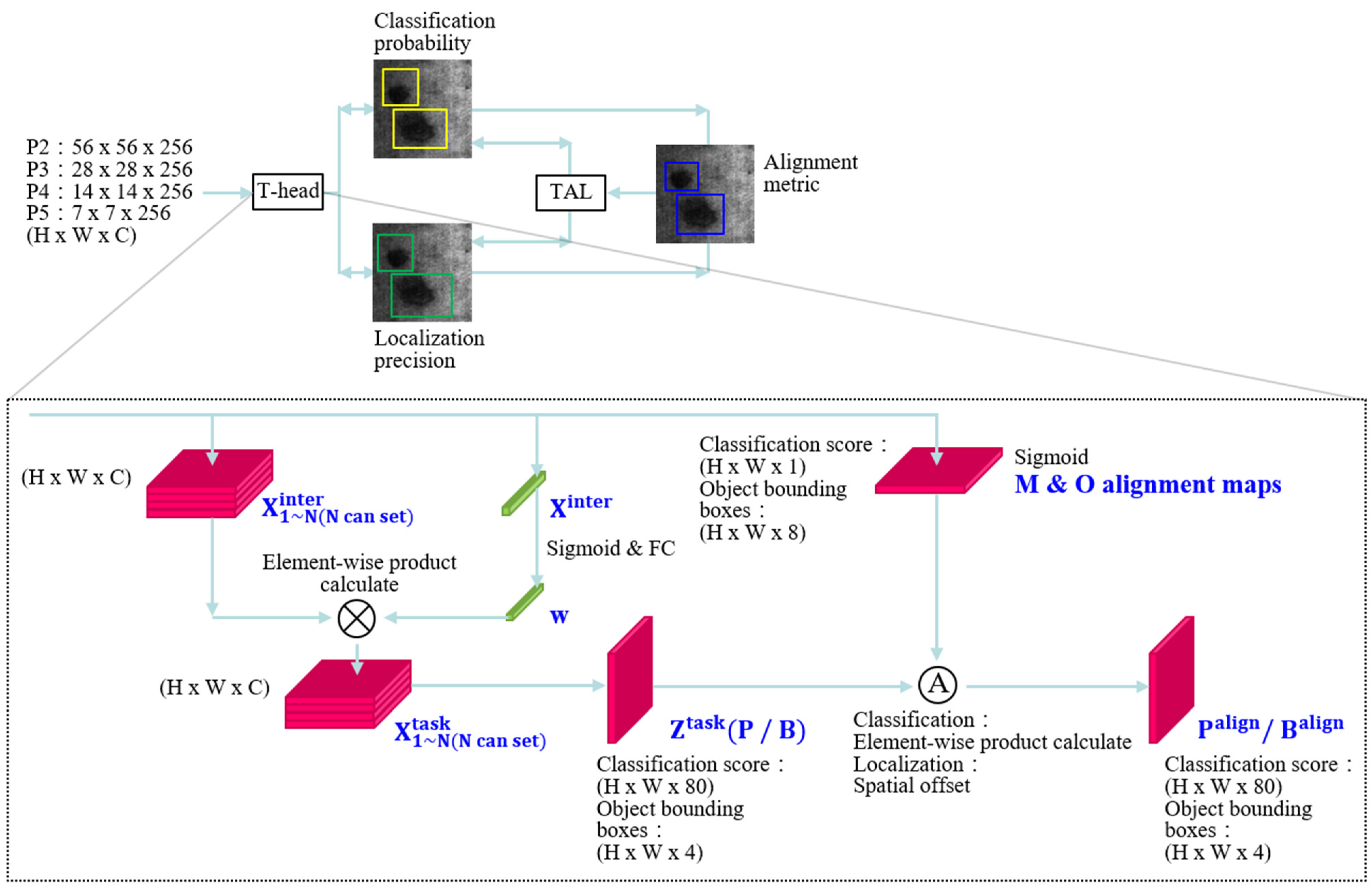
3.4. Task-Aligned
As shown in Figure 3 above, after capturing the detailed features of the FPN, the anchor and bounding box are generated to classify and locate the components. However, the limitations of previous algorithms, which are generated independently, prevent us from generating better anchors and bounding boxes. Therefore, we add the T-head and TAL from [32]. The T-head generates the anchor and bounding box for class and location. The results generated by the T-head in TAL are then used to calculate the anchor and bounding box that should be adjusted and optimized. Feedback is sent to the T-head with the revised parameters, forming a cycle of progressive optimization of the class and location anchor and bounding box. The following is a complete description of the T-head and TAL.
3.4.1. T-head
The convolution H (kernel height), W (kernel width), and C (channels) are designed in . The same H, W, and C corresponding to the same FPN input generate the same N (settable value) k layers of the executive convolution layer (convk). The activation functions are used once, Ref. [32], as in the following (4):
In addition, as seen in Figure 3, the and other convolutional layer M & O alignment maps are concatenated. The M & O alignment maps are used to receive feedback from TAL and optimize the results of the T-head training, where corresponds to generate w, which is a feature computed from the interactive cross-layer task and can depend on the relationship between layers. It is composed of fc 1/2 two fully connected layers and σ Sigmoid activation functions. Equation (5) [32] is as follows:
Next is the element-wise product of w and . The k of wk represents the number of training levels of k layers. Equation (6) [32] is as follows:
The is concatenated features with , as shown in (7) [32] below. Furthermore, the dimension reduction of 1(kernel height) × 1(kernel width) is applied to conv1, and the classification score is H × W × 80 with Sigmoid activation functions. In Figure 3, P is used as the representation; H × W × 4 is used for the bounding box, and the distance to bounding box is converted, as B in FCOS [30] and ATSS [31] in Figure 3.
Finally, the M & O alignment maps (this convolutional layer is used to receive feedback from TAL and optimize the results of T-head training) and are computed separately for the classification score and the bounding box. The (bounding box of classification score) and (bounding box of location) are calculated by the convolution and tend to be approximated in a continuous cycle.
M & O alignment maps are also used to adjust the best values. The learned spatial offsets optimize the classification and location of the anchor and bounding box to achieve the best-predicted bounding box.
3.4.2. TAL
After the T-head and TAL exchange, TAL completes the final bounding box. NMS will calculate the best bounding box as the final training result of this algorithm, and the metal defects will be classified and located.
In TAL, two points need to be achieved: (1) a high mAP bounding box should be generated; (2) the accuracy probability M of low bounding box objects should be reduced, so the following (8) [32] is designed:
The s represents the classification score; u represents the IoU si value; α and β are the adjustable optimization weights. In the general loss function, cross-entropy is mostly used. However, it cannot effectively solve the imbalance between the easy and hard example learning of metal defect objects in the training images.
Focal loss creates a new function pt in (9) [8]. If y = 1 for a positive sample, the value is p. If the negative sample is otherwise, the value is 1 − p. The FL (pt) in (10) [8] is the calculated loss. Its right-constant equation predicts the object classification average precision (AP). The higher the AP, the closer the pt is to the easy example of 1. The lower the AP, the closer the pt is to the hard example of 0.
can effectively adjust the learning weights of easy examples and hard examples downward. In the hard sample case, the FL (pt) is smaller than the cross-entropy calculated by CE (pt). In the easy sample case, FL (pt) is larger than the cross-entropy calculated by CE (pt). FL (pt) adjusts the loss to reduce the problem that hard samples are not easy to train, and it can be used with different settings of α and γ constants to find the best solution for the calculation of mAP. Using the same settings as in [28] and comparing the different mAP results with the various settings in [8], both journals obtained the highest mAP when using α = 0.25 and γ = 2.
Focal loss was applied to TAL and adjusted. The corresponding loss function Lcls can be used to evaluate the classification effect during the training period. Furthermore, Lreg predicts the loss function of the bounding box, and the generalized intersection over union (GIoU) [40] is used instead of IoU.
TAL Loss = Lcls + Lreg
As in (11) [32], Lcls and Lreg are summed to TAL Loss, which is used to evaluate the effectiveness of the training results. It is also used to provide feedback on the anchor and bounding box of the T-head adjustment optimization.
3.5. Soft-NMS
NMS filters all types of object boxes bi (bounding boxes) in a cyclic process. The predicted bounding boxes are first sorted in descending order of their probability of accuracy M. The box with the highest probability of object accuracy is selected as the proposal bounding box, and the remaining boxes are calculated with the other proposal bounding boxes to obtain the IoU value of si. If si is larger than Nt (threshold), then the proposal bounding boxes are discarded, and si is set to 0 and will not be used later. Only the other proposal bounding boxes are kept, and then the comparison process is continued in descending order of probability as described above. Therefore, only the largest box is kept as the proposal bounding box, and the remaining boxes are abandoned. NMS is as shown below (12) [33].
NMS simply drops the proposal bounding box when the si value is larger than the Nt and sets si to 0. The two neighboring or overlapping proposal bounding boxes will have a high probability M that one of the two proposal bounding boxes will be dropped, which will result in a missed detection. The experimental Soft-NMS is used as follows (13) [33] to improve this problem. For the bounding box with overlapping objects, the overlapping area is larger. The equation that modifies si to 0 changes the value of si to tend to 0 but still keeps the bounding box. Therefore, the overlapping of the bounding box objects in mAP can be improved effectively.
4. Experiments and Results
4.1. Implementation Details
4.1.1. Experimental Platform
In the experiment, a 12th Gen Inter(R) Core i7-12700F CPU, NVIDIA GeForce RTX 3080 (with 12 GB memory), CUDA 11.3, and cuDNN 8.2.0 in the Windows 11 environment were used. Anaconda3 2.2.0 was used to build the environment package, and PyCharm Professional Edition 2022.2.1 was used as the experimental platform for the PyTorch 1.11.0 program.
4.1.2. Experimental Parameters
We chose a stochastic gradient descent optimizer (SGD) with 0.9 momentum and 0.001 weight decay. The initial learning rate and total epochs were set as 0.01 and 30 for the metal defect dataset.
4.2. Datasets
The NEU-DET metal defect dataset is a public defect classification dataset proposed by Northeastern University in China in 2013 [1]. There are 300 images for each metal defect classification, and the six types of defects include patches, scratches, pitted surface, crazing, inclusion, and rolled in scale. A total of 1800 images are available, each at 200 × 200 pixels, in jpg file format.
However, each metal defect image may consist of a single defect, or there may be multiple defects in a single image. The dataset provides xml files for the ground truth location and class annotations. Each image is labeled with a ground truth class and a bounding box, for a total of nearly 5000 ground truth boxes.
The experiments used an 8:2 setting in the train image (verification image, of which 1440 metal defect images were used for training) and kept 360 images for training to verify the training results with the loss of truth. The original NEU-DET metal defect dataset is in Pascal VOC format (xml file) and adjusted to YOLO format (txt file) as the training dataset.
4.3. Evaluation Metrics
In this experiment, mAP was used to evaluate the results. The mAP was developed from two important metrics: Recall and Precision. These metrics are defined as follows. TP is the true positive cases (defective objects detected correctly), FP is the false positive cases (non-defective objects detected as defective), and FN is the false negative cases (defective objects that should have been detected but were not detected). Equations (14)–(16) are as follows:
Each defect has an AP number of values, and the mean of the APs of the six defects in this NEU-DET metal defect dataset is mAP. The mAP assesses the total metal defect detection performance index of the proposed algorithm.
4.4. Experiment Results and Analysis
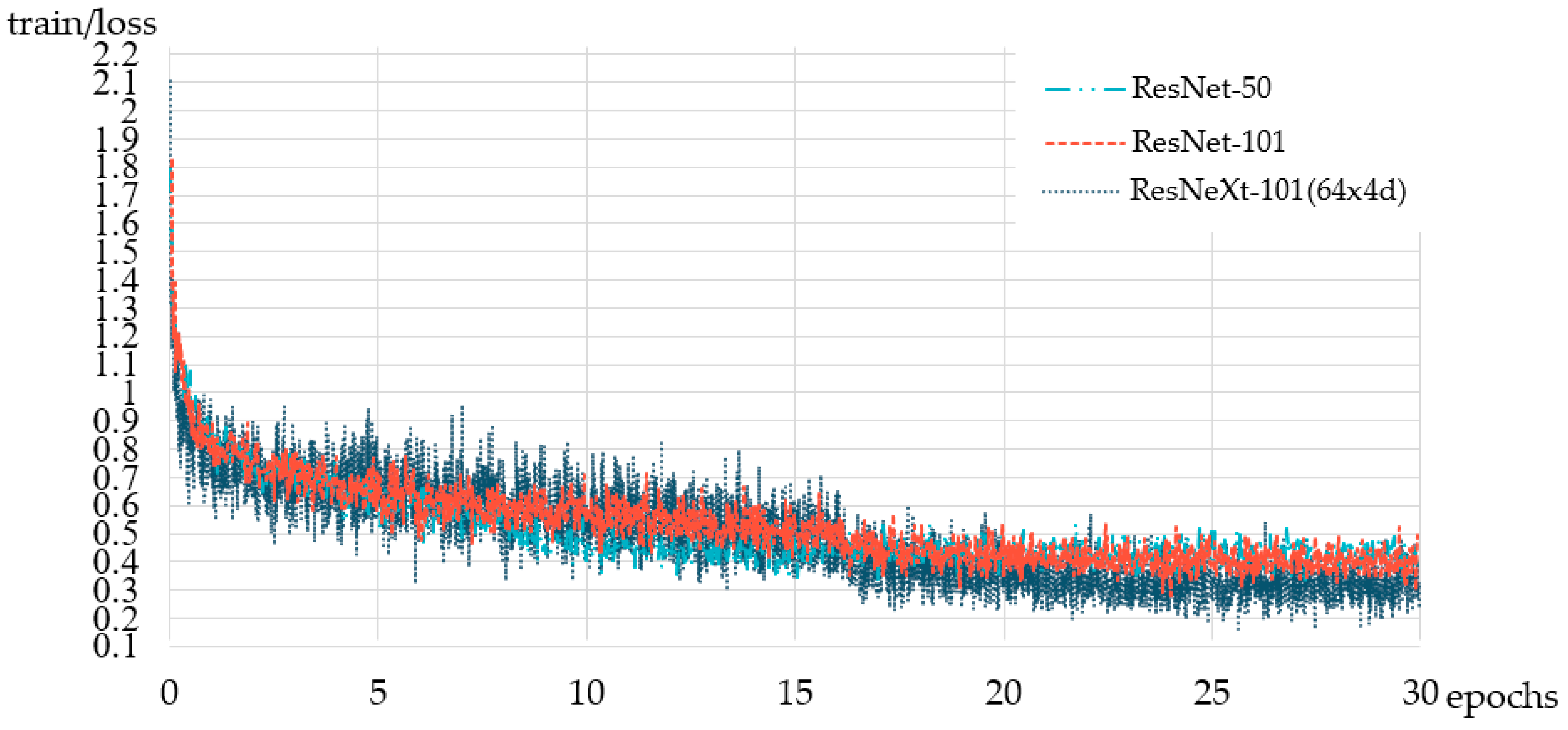
4.4.1. ResNet-50, ResNet-101, and ResNeXt-101
ResNeXt-101 [39] is generally preferred for the backbone due to its grouped convolutions method. ResNeXt-101 is considered to be superior to ResNet-50/101/152 [38], ResNet-200 [41], Inception-v3 [42], and Inception-ResNet-v2 [43] backbones.
The general ResNet-50/101/152 is designed with 1 × 64 d; 1 indicates the number of cardinalities, which is the size of the width of the constructed model, and the higher the number, the better, as researched by [39]. In addition, 64 d indicates the width of the bottleneck; as long as it is higher than 4 d, there is no longer a better mAP. Therefore, in the design of ResNeXt-101, a 64 × 4 d architecture should theoretically improve mAP.
As shown in Table 1, the mAP of ResNeXt-101 (64 × 4 d) was found to be 1.1% lower than that of ResNet-101 in the experiment. We believe that the reason for this is that the number of training parameters required for ResNeXt-101 (64 × 4 d) is twice that of ResNet-101. The corresponding batch size was changed from 6 to 2 in the same training environment, making it impossible to improve the mAP in training.
In addition, it can be seen in Figure 4 that the ResNeXt-101 (64 × 4 d) Loss value fluctuates more and more during training, and it is difficult to converge.
4.4.2. Anchor-Based and Anchor-Free
The TOOD algorithm [32] aims to surpass ATSS [31]. It is considered in ATSS that Anchor-based and Anchor-free cause different differences in mAP. The new architecture designed by ATSS can be used to make Anchor-based and Anchor-free mAPs converge better.
The experimental TOOD algorithm is shown in Table 2, which should be better than the ATSS algorithm. The difference between Anchor-based and Anchor-free experiments is still 0.7% mAP, which is much higher than the difference of 0.1% mAP between Anchor-based and Anchor-free experiments with the ATSS algorithm.
We believe that the reason Anchor-free may outperform Anchor-based is due to the ability of Anchor-free approaches to make more flexible adjustments to anchor scales. This flexibility allows Anchor-free methods to effectively handle defects of various sizes in metal defect detection, resulting in an additional 0.7% mAP. Therefore, Anchor-free was used in our subsequent experiments for further optimization.
4.4.3. IoU Threshold Adjustment for NMS and Soft-NMS
As shown in Table 3 below, DCNv2 C3-C5 was used on ResNet-101 as the backbone. First, the IoU threshold of general NMS was adjusted, and it was found that the mAP was almost unchanged compared to Soft-NMS when setting 0.55 and 0.6. The effect on Soft-NMS is obvious, with an improvement of 0.7% mAP.
In addition, as seen in Table 3 above, choosing the appropriate IoU threshold can improve mAP. There is a certain degree of improvement, but there is still a limit, and the threshold has to be adjusted downward. It can be found that mAP is worse at IoU 0.65 compared to 0.60 mAP, and only gradually to IoU 0.55 or this hour, mAP will be better. However, it can be adjusted to IoU 0.55, 0.5, 0.45, and finally 0.45 to obtain the maximum 77.9% mAP. If we proceed to 0.4, the mAP drops by 1.2%, as shown in Figure 5.
4.4.4. Result
4.5. Ablative Study
The experiments used an ablative study to confirm the effect of DCNv2 between C3-C5 and C4-C5, as shown in Table 5. It was found that mAP was only 76.2% when no DCNv2 was added. When DCNv2 C4-C5 was added, the mAP decreased slightly by 0.1% to 76.1%. The effect is better with the addition of DCNv2 C3, with an improvement of up to 1.0% mAP. We believe that the possible reason is that there are important features in the initial convolution layer of the defective features, which can be used to improve the mAP by the DCNv2 C3 convolution layer.
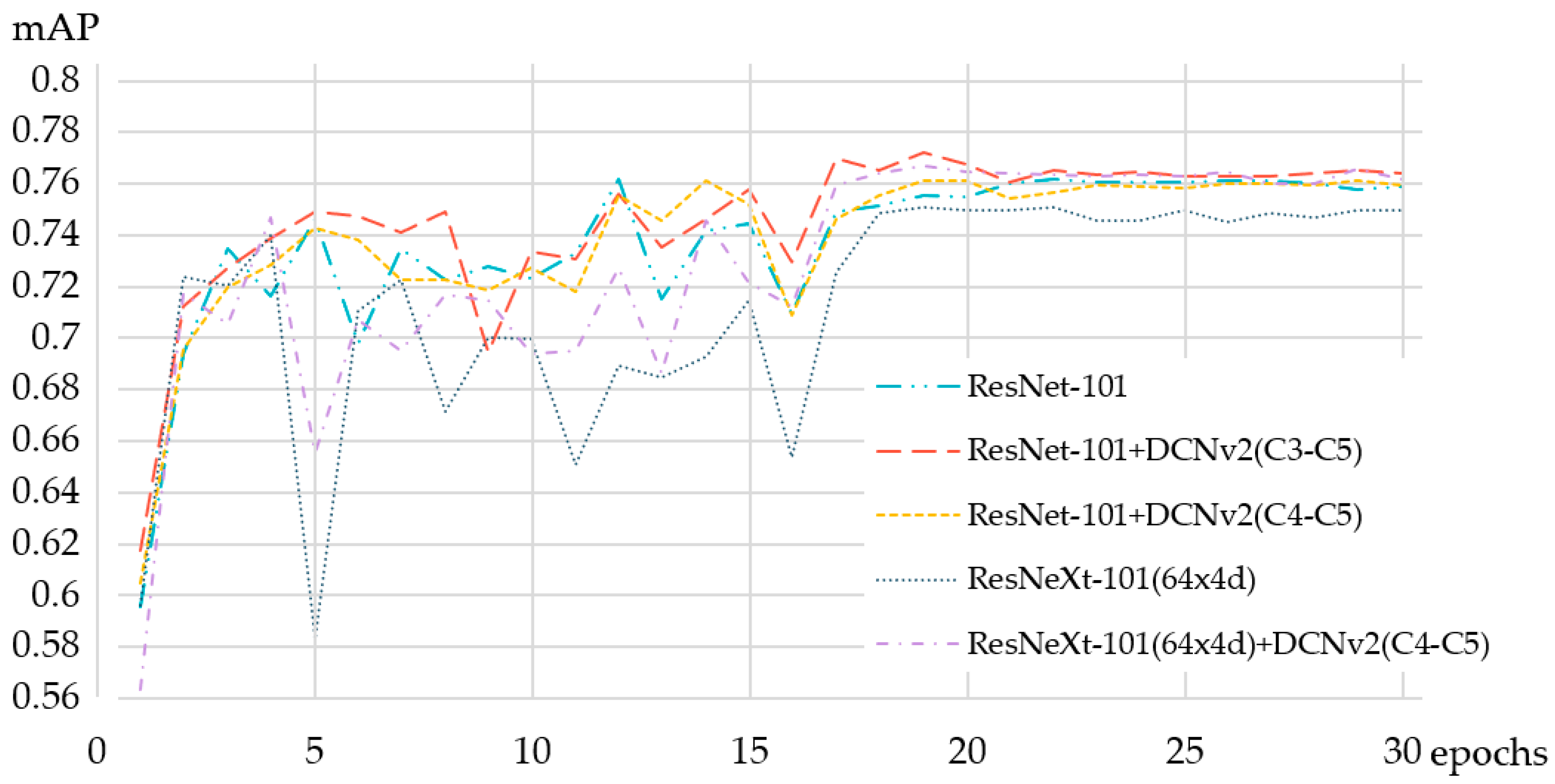
Additionally, an experiment on ResNeXt-101 (64 × 4 d), as shown in Table 6, found that ResNeXt + DCNv2 C4-C5 can increase the mAP up to 1.6% compared to ResNeXt with excellent results. However, ResNeXt + DCNv2 C4-C5 only increases the mAP by 0.5% compared to ResNet + DCNv2 C4-C5. However, compared to ResNet-101 + DCNv2 C3-C5, the mAP is still 0.5% lower, ResNeXt could not produce an advantage in the experiment, and the training time was much longer than ResNet. Under the consideration of time efficiency and mAP, ResNet was chosen as the backbone.
In the following experiment (Figure 7), it is shown that ResNet-101 + DCNv2 C3-C5 can have a smooth and high mAP at the beginning of training. During the subsequent training period, no overfitting occurred, and the verified mAP gradually increased to 77.2%.
4.6. Comparison with State-of-the-Art
The experiments refer to other mAPs experimented on in the journal using the metallic defect NEU-DET dataset. Data include those provided in [6,8,9] and also compared with well-known algorithms such as M2Det-320 [44], YOLOv3 [45], YOLOv4 [46], YOLOv5 [12], YOLOv7 [47], YOLOv8 [12], EfficientDet [48], and SAPD [49].
As shown in Table 7, mAP is only in the top class but not outstanding in the three types of metal defect patches, scratches, and crazing by the TAMD algorithm. However, the TAMD model has lower performance in detecting pitted surface and rolled-in scale defects; thus, compared to other models, the TAMD model may struggle to effectively recognize non-continuous metal defect features, which results in lower mAP. The TAMD model performs first on inclusion, a relatively complex feature, with a mAP of 82.8%. On average, our TAMD algorithm outperforms other algorithms with 77.9% mAP and 0.6% more than the second place YOLOv8.
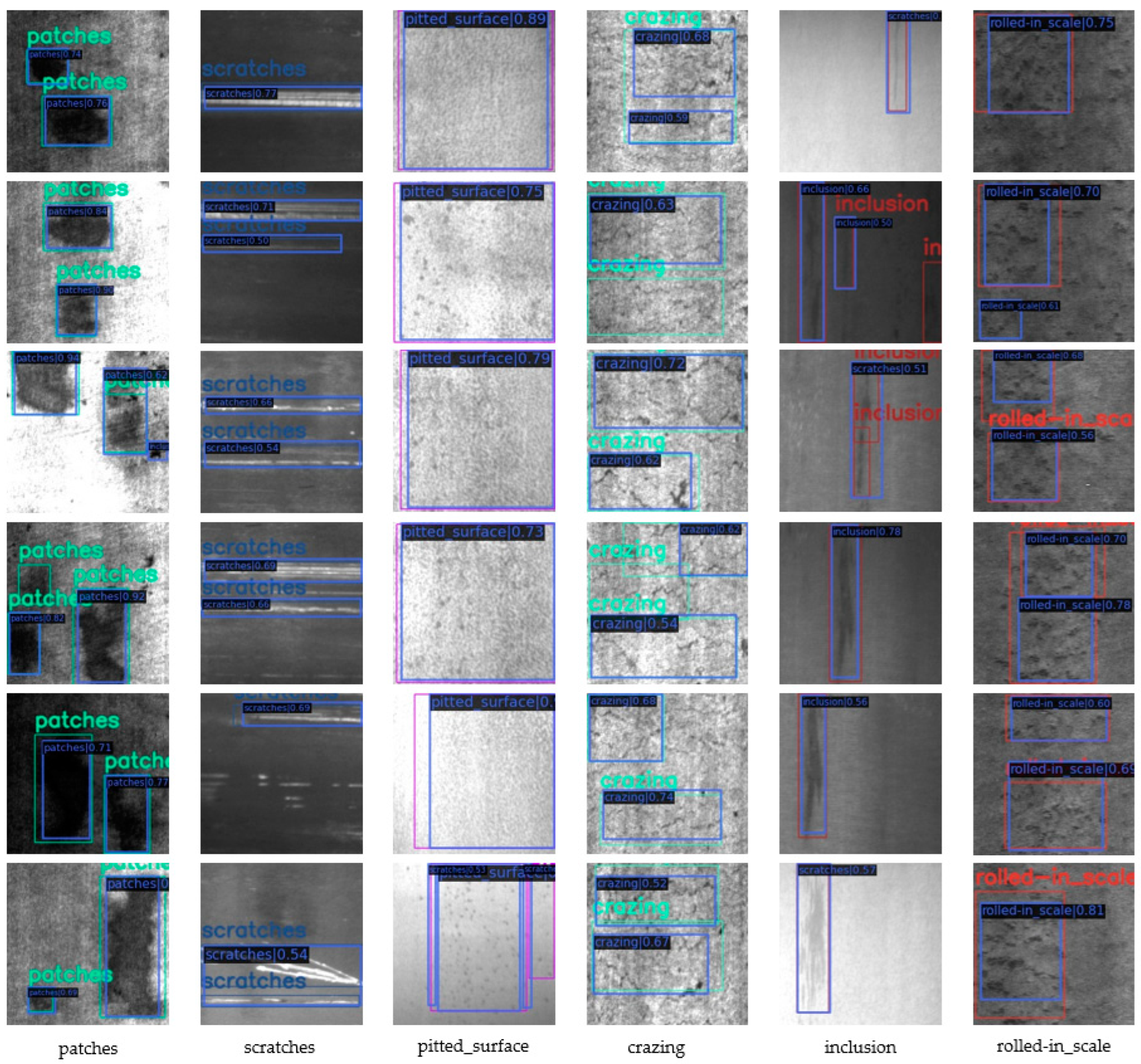
The experiments using the TAMD algorithm to detect the defective objects are shown in Figure 8. It was found that the four types of metal defects—patches, scratches, pitted surface, and inclusion—are well mapped and can be classified correctly, and the size of the bounding box is almost correct. However, the mAP was lower for crazing and rolled-in scale. It was also found that the ground truth bounding box is hard to recognize and frame by the human eye in crazing and rolled in scale, and it is also found that the ground truth bounding box of the NEU-DET dataset is not entirely correct. There is a lot of space for discussion, and this may be a future improvement.
5. Conclusions
Compared with other advanced models, our TAMD model has a higher mAP and better performance in some metal defect classes. In various experiments, we used ResNet-101 as the backbone with variable convolution between the DCNv2 C3-C5 layers to classify and localize metal defects, which is the first use of the TOOD model for metal defects. First, we adopted the task-aligned approach to constantly modify and optimize the anchor and bounding box of objects and classifications and, finally, Soft-NMS to improve the IoU and adjust the threshold. We obtained a 2.5% increase in mAP from 75.4% to 77.9% and a 0.6% increase in mAP compared to existing advanced algorithms such as YOLOv8 mAP. However, the TAMD model still has limitations; for example, the detection of pitted_ surface and roller-in scale cannot effectively recognize the continuous metal defect features, which leads to lower performance.
In terms of future planning, there are three directions as follows: (1) in terms of algorithm optimization, there are still more areas worth testing and adjusting; (2) in metal defective images, image enhancement will be considered for development at the input side, in the hope that mAP can be more improved; (3) in other defective object scenes for application, the effectiveness of the TAMD algorithm will be explored.
Author Contributions
Conceptualization, C.-H.K.; Methodology, C.-H.K.; Software, M.-H.H.; Validation, M.-H.H.; Formal analysis, C.-H.K.; Investigation, C.-H.K.; Resources, K.-Y.C.; Writing—original draft, C.-H.K.; Writing—review & editing, M.-H.H.; Visualization, C.-H.K.; Supervision, K.-Y.C.; Project administration, M.-H.H. All authors have read and agreed to the published version of the manuscript.
Funding
This research received no external funding.
Data Availability Statement
The data presented in this study are openly available.
Conflicts of Interest
The authors declare no conflict of interest.
References
- Song, K.; Yan, Y. A noise robust method based on completed local binary patterns for hot-rolled steel strip surface defects. Appl. Surf. Sci. 2013, 285, 858–864. [Google Scholar] [CrossRef]
- Wang, L. Support Vector Machines: Theory and Applications; Springer: Berlin/Heidelberg, Germany, 2005; pp. 159–179. [Google Scholar]
- Breiman, L. Random Forests. Mach. Learn. 2001, 45, 5–32. [Google Scholar] [CrossRef]
- Smith, L.I. A Tutorial on Principal Components Analysis. 2002. Available online: https://www.semanticscholar.org/paper/A-tutorial-on-Principal-Components-Analysis-Smith/462bf829634e3ffaef794de5e58809994d30f8ec (accessed on 2 September 2023).
- Abeywickrama, T.; Aamir Cheema, M.; Taniar, D. k-Nearest Neighbors on Road Networks: A Journey in Experimentation and In-Memory Implementation. arXiv 2016, arXiv:1601.01549. [Google Scholar] [CrossRef]
- Wang, W.; Mi, C.; Wu, Z.; Lu, K.; Long, H.; Pan, B.; Li, D.; Zhang, J.; Chen, P.; Wang, B. A Real-Time Steel Surface Defect Detection Approach With High Accuracy. IEEE Trans. Instrum. Meas. 2022, 71, 1357. [Google Scholar] [CrossRef]
- He, Y.; Song, K.; Meng, Q.; Yan, Y. An End-to-End Steel Surface Defect Detection Approach via Fusing Multiple Hierarchical Features. IEEE Trans. Instrum. Meas. 2020, 69, 1493–1504. [Google Scholar] [CrossRef]
- Cheng, X.; Yu, J. RetinaNet With Difference Channel Attention and Adaptively Spatial Feature Fusion for Steel Surface Defect Detection. IEEE Trans. Instrum. Meas. 2021, 70, 2503911. [Google Scholar] [CrossRef]
- Yu, J.; Cheng, X.; Li, Q. Surface Defect Detection of Steel Strips Based on Anchor-Free Network With Channel Attention and Bidirectional Feature Fusion. IEEE Trans. Instrum. Meas. 2022, 71, 5000710. [Google Scholar] [CrossRef]
- Li, Z.; Tian, X.; Liu, X.; Liu, Y.; Shi, X. A Two-Stage Industrial Defect Detection Framework Based on Improved-YOLOv5 and Optimized-Inception-ResnetV2 Models. Appl. Sci. 2022, 12, 834. [Google Scholar] [CrossRef]
- Lv, X.; Duan, F.; Jiang, J.J.; Fu, X.; Gan, L. Deep Metallic Surface Defect Detection: The New Benchmark and Detection Network. Sensors 2020, 20, 1562. [Google Scholar] [CrossRef]
- Wang, J.; Xu, P.; Li, L.; Zhang, F. DAssd-Net: A Lightweight Steel Surface Defect Detection Model Based on Multi-Branch Dilated Convolution Aggregation and Multi-Domain Perception Detection Head. Sensors 2023, 23, 5488. [Google Scholar] [CrossRef]
- Niu, M.; Wang, Y.; Song, K.; Wang, Q.; Zhao, Y.; Yan, Y. An Adaptive Pyramid Graph and Variation Residual-Based Anomaly Detection Network for Rail Surface Defects. IEEE Trans. Instrum. Meas. 2021, 70, 5020013. [Google Scholar] [CrossRef]
- Yang, H.; Wang, Y.; Hu, J.; He, J.; Yao, Z.; Bi, Q. Deep Learning and Machine Vision-Based Inspection of Rail Surface Defects. IEEE Trans. Instrum. Meas. 2022, 71, 5005714. [Google Scholar] [CrossRef]
- Jin, X.; Wang, Y.; Zhang, H.; Zhong, H.; Liu, L.; Wu, Q.M.J.; Yang, Y. DM-RIS: Deep Multimodel Rail Inspection System With Improved MRF-GMM and CNN. IEEE Trans. Instrum. Meas. 2020, 69, 1051–1065. [Google Scholar] [CrossRef]
- Nieniewski, M. Morphological Detection and Extraction of Rail Surface Defects. IEEE Trans. Instrum. Meas. 2020, 69, 6870–6879. [Google Scholar] [CrossRef]
- Su, B.; Chen, H.; Liu, K.; Liu, W. RCAG-Net: Residual Channelwise Attention Gate Network for Hot Spot Defect Detection of Photovoltaic Farms. IEEE Trans. Instrum. Meas. 2021, 70, 3510514. [Google Scholar] [CrossRef]
- Tao, X.; Zhang, D.; Hou, W.; Ma, W.; Xu, D. Industrial Weak Scratches Inspection Based on Multifeature Fusion Network. IEEE Trans. Instrum. Meas. 2021, 70, 5000514. [Google Scholar] [CrossRef]
- Krizhevsky, A.; Sutskever, I.; Hinton, G.E. Imagenet classification with deep convolutional neural networks. Commun. ACM 2017, 60, 84–90. [Google Scholar] [CrossRef]
- Sermanet, P.; Eigen, D.; Zhang, X.; Mathieu, M.; Fergus, R.; LeCun, Y. OverFeat: Integrated Recognition, Localization and Detection using Convolutional Networks. arXiv 2013, arXiv:1312.6229. [Google Scholar]
- Redmon, J.; Divvala, S.; Girshick, R.; Farhadi, A. You Only Look Once: Unified, Real-Time Object Detection. In Proceedings of the 2016 IEEE Conference on Computer Vision and Pattern Recognition (CVPR), Las Vegas, NV, USA, 27–30 June 2016; pp. 779–788. [Google Scholar]
- Liu, W.; Anguelov, D.; Erhan, D.; Szegedy, C.; Reed, S.; Fu, C.-Y.; Berg, A.C. SSD: Single Shot MultiBox Detector. In Proceedings of the Computer Vision—ECCV 2016, Amsterdam, The Netherlands, 11–14 October 2016; pp. 21–37. [Google Scholar]
- Girshick, R.; Donahue, J.; Darrell, T.; Malik, J. Rich Feature Hierarchies for Accurate Object Detection and Semantic Segmentation. In Proceedings of the 2014 IEEE Conference on Computer Vision and Pattern Recognition, Columbus, OH, USA, 23–28 June 2014; pp. 580–587. [Google Scholar]
- Girshick, R. Fast R-CNN. In Proceedings of the 2015 IEEE International Conference on Computer Vision (ICCV), Washington, DC, USA, 7–13 December 2015; pp. 1440–1448. [Google Scholar]
- Ren, S.; He, K.; Girshick, R.; Sun, J. Faster R-CNN: Towards Real-Time Object Detection with Region Proposal Networks. arXiv 2015, arXiv:1506.01497. [Google Scholar] [CrossRef]
- Cai, Z.; Vasconcelos, N. Cascade R-CNN: Delving into High Quality Object Detection. In Proceedings of the 2018 IEEE/CVF Conference on Computer Vision and Pattern Recognition, Salt Lake City, UT, USA, 18–23 June 2018; pp. 6154–6162. [Google Scholar]
- Lin, T.-Y.; Dollar, P.; Girshick, R.; He, K.; Hariharan, B.; Belongie, S. Feature Pyramid Networks for Object Detection. In Proceedings of the 2017 IEEE Conference on Computer Vision and Pattern Recognition (CVPR), Honolulu, HI, USA, 21–26 July 2017; pp. 936–944. [Google Scholar]
- Lin, T.Y.; Goyal, P.; Girshick, R.; He, K.; Dollár, P. Focal Loss for Dense Object Detection. In Proceedings of the 2017 IEEE International Conference on Computer Vision (ICCV), Venice, Italy, 22–29 October 2017; pp. 2999–3007. [Google Scholar]
- Duan, K.; Bai, S.; Xie, L.; Qi, H.; Huang, Q.; Tian, Q. CenterNet: Keypoint Triplets for Object Detection. In Proceedings of the 2019 IEEE/CVF International Conference on Computer Vision (ICCV), Seoul, Republic of Korea, 27 October–2 November 2019; pp. 6568–6577. [Google Scholar]
- Tian, Z.; Shen, C.; Chen, H.; He, T. FCOS: Fully Convolutional One-Stage Object Detection. In Proceedings of the 2019 IEEE/CVF International Conference on Computer Vision (ICCV), Seoul, Republic of Korea, 27 October–2 November 2019; pp. 9626–9635. [Google Scholar]
- Zhang, S.; Chi, C.; Yao, Y.; Lei, Z.; Li, S.Z. Bridging the Gap Between Anchor-Based and Anchor-Free Detection via Adaptive Training Sample Selection. In Proceedings of the 2020 IEEE/CVF Conference on Computer Vision and Pattern Recognition (CVPR), Seattle, WA, USA, 13–19 June 2020; pp. 9756–9765. [Google Scholar]
- Feng, C.; Zhong, Y.; Gao, Y.; Scott, M.R.; Huang, W. TOOD: Task-aligned One-stage Object Detection. In Proceedings of the 2021 IEEE/CVF International Conference on Computer Vision (ICCV), Montreal, BC, Canada, 11–17 October 2021; pp. 3490–3499. [Google Scholar]
- Bodla, N.; Singh, B.; Chellappa, R.; Davis, L.S. Soft-NMS—Improving Object Detection with One Line of Code. In Proceedings of the 2017 IEEE International Conference on Computer Vision (ICCV), Venice, Italy, 22–29 October 2017; pp. 5562–5570. [Google Scholar]
- Zhu, X.; Hu, H.; Lin, S.; Dai, J. Deformable ConvNets V2: More Deformable, Better Results. In Proceedings of the 2019 IEEE/CVF Conference on Computer Vision and Pattern Recognition (CVPR), Long Beach, CA, USA, 15–20 June 2019; pp. 9300–9308. [Google Scholar]
- Dai, J.; Qi, H.; Xiong, Y.; Li, Y.; Zhang, G.; Hu, H.; Wei, Y. Deformable Convolutional Networks. In Proceedings of the 2017 IEEE International Conference on Computer Vision (ICCV), Venice, Italy, 22–29 October 2017; pp. 764–773. [Google Scholar]
- Hosang, J.; Benenson, R.; Schiele, B. Learning Non-maximum Suppression. In Proceedings of the 2017 IEEE Conference on Computer Vision and Pattern Recognition (CVPR), Honolulu, HI, USA, 21–26 July 2017; pp. 6469–6477. [Google Scholar]
- Lin, T.-Y.; Maire, M.; Belongie, S.; Hays, J.; Perona, P.; Ramanan, D.; Dollár, P.; Zitnick, C.L. Microsoft COCO: Common Objects in Context. In Proceedings of the Computer Vision—ECCV 2014, Zurich, Switzerland, 6–12 September 2014; pp. 740–755. [Google Scholar]
- He, K.; Zhang, X.; Ren, S.; Sun, J. Deep Residual Learning for Image Recognition. In Proceedings of the 2016 IEEE Conference on Computer Vision and Pattern Recognition (CVPR), Las Vegas, NV, USA, 27–30 June 2016; pp. 770–778. [Google Scholar]
- Xie, S.; Girshick, R.; Dollar, P.; Tu, Z.; He, K. Aggregated Residual Transformations for Deep Neural Networks. In Proceedings of the 2017 IEEE Conference on Computer Vision and Pattern Recognition (CVPR), Honolulu, HI, USA, 21–26 July 2017; pp. 5987–5995. [Google Scholar]
- Rezatofighi, H.; Tsoi, N.; Gwak, J.; Sadeghian, A.; Reid, I.; Savarese, S. Generalized Intersection Over Union: A Metric and a Loss for Bounding Box Regression. In Proceedings of the 2019 IEEE/CVF Conference on Computer Vision and Pattern Recognition (CVPR), Long Beach, CA, USA, 15–20 June 2019; pp. 658–666. [Google Scholar]
- He, K.; Zhang, X.; Ren, S.; Sun, J. Identity Mappings in Deep Residual Networks. In Proceedings of the Computer Vision—ECCV 2016, Amsterdam, The Netherlands, 11–14 October 2016; pp. 630–645. [Google Scholar]
- Szegedy, C.; Vanhoucke, V.; Ioffe, S.; Shlens, J.; Wojna, Z. Rethinking the Inception Architecture for Computer Vision. In Proceedings of the 2016 IEEE Conference on Computer Vision and Pattern Recognition (CVPR), Las Vegas, NV, USA, 27–30 June 2016; pp. 2818–2826. [Google Scholar]
- Szegedy, C.; Ioffe, S.; Vanhoucke, V.; Alemi, A. Inception-v4, Inception-ResNet and the Impact of Residual Connections on Learning. In Proceedings of the AAAI conference on artificial intelligence, San Francisco, CA, USA, 4–9 February 2017; Volume 31. [Google Scholar] [CrossRef]
- Zhao, Q.; Sheng, T.; Wang, Y.; Tang, Z.; Chen, Y.; Cai, L.; Ling, H. M2Det: A Single-Shot Object Detector based on Multi-Level Feature Pyramid Network. arXiv 2018, arXiv:1811.04533. [Google Scholar] [CrossRef]
- Redmon, J.; Farhadi, A. YOLOv3: An Incremental Improvement. arXiv 2018, arXiv:1804.02767. [Google Scholar]
- Bochkovskiy, A.; Wang, C.-Y.; Liao, H.-Y.M. YOLOv4: Optimal Speed and Accuracy of Object Detection. arXiv 2020, arXiv:2004.10934. [Google Scholar]
- Wang, C.-Y.; Bochkovskiy, A.; Liao, H.-Y.M. YOLOv7: Trainable bag-of-freebies sets new state-of-the-art for real-time object detectors. arXiv 2022, arXiv:2207.02696. [Google Scholar]
- Tan, M.; Pang, R.; Le, Q.V. EfficientDet: Scalable and Efficient Object Detection. In Proceedings of the 2020 IEEE/CVF Conference on Computer Vision and Pattern Recognition (CVPR), Seattle, WA, USA, 13–19 June 2020; pp. 10778–10787. [Google Scholar]
- Zhu, C.; Chen, F.; Shen, Z.; Savvides, M. Soft Anchor-Point Object Detection. arXiv 2019, arXiv:1911.12448. [Google Scholar]
Figure 1.
The schematic diagram of the NEU-DET dataset.

Figure 2.
TAMD model architecture.

Figure 3.
Task-aligned architecture.

Figure 4.
Backbone in ResNet-50/101, ResNeXt-101 Loss value comparison diagram.

Figure 5.
Soft-NMS IoU thresholds in ResNet-101 mAP comparison diagram.

Figure 6.
TAMD model training mAP diagram.

Figure 7.
DCNv2 training mAP diagram.

Figure 8.
MATD defect detection result image.


Table 1.
Backbone in ResNet-50/101, ResNeXt-101 map comparison table.
| Backbone | mAP |
|---|---|
| ResNet-50 | 76.1 |
| ResNet-101 | 76.2 |
| ResNeXt-101 (64 × 4 d) | 75.1 |
Table 2.
Anchor-based vs. anchor-free map comparison table.
| Backbone | Anchor | mAP |
|---|---|---|
| ResNet-50 | Anchor-based | 75.4 |
| Anchor-free | 76.1 |
Table 3.
IoU thresholds of NMS and Soft-NMS compared in the ResNet-101 mAP table.
| Backbone | IoU | mAP | |
|---|---|---|---|
| ResNet-101 | NMS | 0.55 | 77.2 |
| NMS | 0.60 | 77.2 | |
| Soft NMS | 0.40 | 76.7 | |
| Soft NMS | 0.45 | 77.9 | |
| Soft NMS | 0.50 | 77.8 | |
| Soft NMS | 0.55 | 77.8 | |
| Soft NMS | 0.60 | 77.1 | |
| Soft NMS | 0.65 | 76.4 | |
Table 4.
TAMD model parameter table.
| Backbone | Anchor | Type | IoU | mAP |
|---|---|---|---|---|
| ResNet-101 | Anchor-free | DCNv2(C3-C5) | Soft NMS 0.45 | 77.9 |
Table 5.
DCNv2 C3-C5 and DCNv2 C4-C5 in ResNet-101 mAP comparison table.
| DCNv2 (C3-C5) | DCNv2 (C4-C5) | Backbone | mAP | Baseline |
|---|---|---|---|---|
| ResNet-101 | 76.2 | - | ||
| V | ResNet-101 | 77.2 | +1.0 | |
| V | ResNet-101 | 76.1 | −0.1 |
Table 6.
DCNv2 C4-C5 in ResNet-101 and ResNeXt-101 (64 × 4 d) mAP comparison table.
| DCNv2 (C4-C5) | Backbone | mAP | Baseline |
|---|---|---|---|
| ResNet-101 | 76.2 | - | |
| V | ResNet-101 | 76.1 | −0.1 |
| ResNeXt-101 (64 × 4 d) | 75.1 | −1.1 | |
| V | ResNeXt-101 (64 × 4 d) | 76.7 | +0.5 |
Table 7.
Comparison with other models mAP and AP.
| Model | mAP | Patches AP | Scratches AP | Pitted_ Surface AP | Crazing AP | Inclusion AP | Roller- in Scale AP |
|---|---|---|---|---|---|---|---|
| M2Det-320 [43] | 61.1 | 81.7 | 70.8 | 72.0 | 28.5 | 64.9 | 48.4 |
| ATSS [6] | 67.8 | 85.8 | 81.8 | 75.7 | 33.0 | 70.8 | 59.6 |
| YOLOv3 [44] | 69.4 | 71.4 | 73.7 | 68.3 | 68.4 | 61.9 | 72.3 |
| EifficientDet [45] | 70.1 | 83.5 | 73.1 | 85.5 | 45.9 | 62.0 | 72.7 |
| Improved YOLOv3 [6] | 70.7 | 84.9 | 92.1 | 87.8 | 24.8 | 72.1 | 62.3 |
| FCOS [6] | 71.3 | 86.5 | 78.2 | 79.8 | 44.1 | 76.1 | 63.3 |
| SAPD [46] | 73.2 | 93.9 | 97.8 | 87.4 | 44.6 | 73.3 | 42.9 |
| Cascade [6] | 73.3 | 88.4 | 88.2 | 81.3 | 38.3 | 76.0 | 67.8 |
| YOLOv4 [47] | 74.6 | 92.5 | 77.9 | 83.6 | 64.9 | 74.2 | 54.3 |
| SSD300 [6] | 74.8 | 90.6 | 84.1 | 83.8 | 46.9 | 75.9 | 67.3 |
| Improved Faster R-CNN [8] | 74.8 | 89.1 | 83.4 | 82.1 | 52.2 | 77.3 | 64.7 |
| YOLOv5-s [12] | 75.0 | 87.0 | 92.0 | 90.0 | 30.0 | 79.0 | 72.0 |
| RetinaNet [9] | 75.3 | 93.3 | 73.5 | 91.4 | 53.0 | 78.7 | 62.0 |
| YOLOv5-v6.1-s [12] | 75.5 | 85.0 | 92.0 | 91.0 | 38.0 | 82.0 | 65.0 |
| YOLOv7-tiny [12] | 75.6 | 86.0 | 95.0 | 86.0 | 42.0 | 77.0 | 69.0 |
| CABF-FCOS [9] | 76.7 | 93.5 | 84.4 | 88.9 | 55.4 | 75.0 | 62.9 |
| CenterNet [6] | 77.1 | 91.4 | 94.2 | 87.4 | 44.2 | 82.7 | 62.9 |
| YOLOv8-s [12] | 77.3 | 91.0 | 93.0 | 92.0 | 43.0 | 84.0 | 60.0 |
| TAMD (Ours) | 77.9 | 92.0 | 92.4 | 82.6 | 56.8 | 82.8 | 60.5 |
Disclaimer/Publisher’s Note: The statements, opinions and data contained in all publications are solely those of the individual author(s) and contributor(s) and not of MDPI and/or the editor(s). MDPI and/or the editor(s) disclaim responsibility for any injury to people or property resulting from any ideas, methods, instructions or products referred to in the content. |
© 2023 by the authors. Licensee MDPI, Basel, Switzerland. This article is an open access article distributed under the terms and conditions of the Creative Commons Attribution (CC BY) license (https://creativecommons.org/licenses/by/4.0/).
Share and Cite
MDPI and ACS Style
Hung, M.-H.; Ku, C.-H.; Chen, K.-Y. Application of Task-Aligned Model Based on Defect Detection. Automation 2023, 4, 327-344. https://0-doi-org.brum.beds.ac.uk/10.3390/automation4040019
AMA Style
Hung M-H, Ku C-H, Chen K-Y. Application of Task-Aligned Model Based on Defect Detection. Automation. 2023; 4(4):327-344. https://0-doi-org.brum.beds.ac.uk/10.3390/automation4040019
Chicago/Turabian StyleHung, Ming-Hung, Chao-Hsun Ku, and Kai-Ying Chen. 2023. "Application of Task-Aligned Model Based on Defect Detection" Automation 4, no. 4: 327-344. https://0-doi-org.brum.beds.ac.uk/10.3390/automation4040019