Identifying the Input Uncertainties to Quantify When Prioritizing Railway Assets for Risk-Reducing Interventions


Institute of Construction and Infrastructure Management, ETH Zurich, Stefano-Franscini-Platz 5, 8093 Zürich, Switzerland
*
Author to whom correspondence should be addressed.
CivilEng 2020, 1(2), 106-131; https://0-doi-org.brum.beds.ac.uk/10.3390/civileng1020008
Submission received: 12 July 2020
/
Revised: 13 August 2020
/
Accepted: 13 August 2020
/
Published: 19 August 2020
(This article belongs to the Special Issue Addressing Risk in Engineering Asset Management)
Abstract
:Railway managers identify and prioritize assets for risk-reducing interventions. This requires the estimation of risks due to failures, as well as the estimation of costs and effects due to interventions. This, in turn, requires the estimation of values of numerous input variables. As there is uncertainty related to the initial input estimates, there is uncertainty in the output, i.e., assets to be prioritized for risk-reducing interventions. Consequently, managers are confronted with two questions: Do the uncertainties in inputs cause significant uncertainty in the output? If so, where should efforts be concentrated to quantify them? This paper discusses the identification of input uncertainties that are likely to affect railway asset prioritization for risk-reducing interventions. Once the track sections, switches and bridges of a part of the Irish railway network were prioritized using best estimates of inputs, they were again prioritized using: (1) reasonably low and high estimates, and (2) Monte Carlo sampling from skewed normal distributions, where the low and high estimates encompass the 95% confidence interval. The results show that only uncertainty in a few inputs influences the prioritization of the assets for risk-reducing interventions. Reliable prioritization of assets can be achieved by quantifying the uncertainties in these particular inputs.
1. Introduction
Railway managers are responsible for planning and executing risk-reducing interventions. To achieve this, they must estimate the risks due to failures as well as the costs and effects on service due to interventions for all the assets and then prioritize their interventions accordingly. There is a plethora of methods and models to estimate the risks due to railway asset failures, as well as the costs and effects on rail service due to failures and interventions. For example, [1,2,3,4,5,6,7,8,9,10,11,12] analyze the risk related to railways due to specific hazards. Many scholars have focused on the analysis of risk related to specific failure modes of the railway assets, e.g., [13,14,15,16,17,18,19,20,21,22,23,24,25,26,27]. Other scholars have investigated the occurrence of specific effects on the service, such as accidents (e.g., [28,29,30,31,32,33,34,35,36]), and delays (e.g., [37,38]).
The value of numerous variables must be determined to estimate the risks, costs, and effects on service due to failures and interventions to prioritize risk-reducing interventions. Railway managers often use a point value to represent the best estimate of an input variable. This best estimate of an input can be obtained using expert knowledge (e.g., [39,40,41,42,43,44,45]), historical data (e.g., [46,47,48,49,50]), or models (e.g., [51,52,53,54]). However, there is often uncertainty in the best estimates, as they are not precise estimations or distribution functions of the inputs. Consequently, once the assets to be prioritized for interventions have been identified using only best estimates of inputs, railway managers need to know if different assets would be prioritized, given the uncertainty in the inputs. To do this, they must examine how sensitive the prioritization of the assets for interventions is to input uncertainties.
In this paper, the term ‘input uncertainties’ refers only to the statistical uncertainties in the input values used to rank the assets for interventions. Although other uncertainties also exist, e.g., in the models used to estimate risks and costs, they are neglected. The input uncertainties, therefore, represent all the unknowns that can cause variations in the values of the input variables required to estimate the risks, costs, and effects due to interventions, which are subsequently used to rank the assets. Although often no distinction is made between the estimation of probabilistic risk and the quantification of uncertainties [55], e.g., in [56,57], in this analysis, such a distinction must be made because the uncertainty in the risk value is considered. To estimate the risk, the values of failure probability and the extent of consequences due to failure must be obtained. The uncertainties in values used to represent the probability and consequences of failure yield uncertainties in the risk value.
The necessity of a systematic consideration of input uncertainties has been widely acknowledged in railway management. Many scholars have investigated the effect of input uncertainties in the estimation of risks due to failures of railway assets (e.g., [32,58,59,60,61,62,63,64,65]), as well as of costs and effects on rail service due to interventions (e.g., [57,66,67,68,69,70,71,72,73]). As there are uncertainties in the estimations of risks, costs, and effects on service, the ranking of assets for interventions, which is based on these estimates, might not be reliable. The effect of the input uncertainties in the ranking of assets must be, therefore, quantified. For example, in [56], the effect of the input uncertainties on the prioritization of risk-reducing interventions for water supply infrastructure is quantified. Other examples of methods to quantify the uncertainty in prioritization problems are [74,75,76].
In practice, however, it is common to neglect the input uncertainties when prioritizing railway assets for interventions [77]. Railway managers know that there is a high cost in quantifying all these uncertainties and then in considering them when planning interventions. To quantify the input uncertainties, one must obtain the complete set of plausible values for each input, from which the probability distribution of each input is built. To consider the input uncertainties when prioritizing assets for interventions, one must first use these distributions to represent each input when modeling the risks, costs, and effects on service for each asset. Then, these results can be used to identify which assets should be prioritized for interventions. This process requires more data, more complex models, and higher computational effort, leading to higher costs than using the best estimates of the inputs.
However, quantifying and considering all the input uncertainties instead of using best estimates is beneficial for the railway managers only if the input uncertainties highly influence the ranking of the assets for interventions. It is reasonable to expect that the ranking of the assets will not be equally sensitive to all input uncertainties. If railway managers know how sensitive the ranking is to each input uncertainty, they can decide which inputs they must quantify and consider when prioritizing risk-reducing interventions. They can also, then, decide for which inputs the use of best estimates delivers reliable results. Railway managers can have a first impression of how likely it is that an input uncertainty affects the ranking of the assets by doing a simple analysis; evaluating how sensitive the ranking produced using only best estimates of inputs is to the use of extreme yet plausible input values as well as to the use of simple distribution functions of inputs.
This paper shows how reasonably extreme estimates of inputs were used, in addition to the best estimates, to identify the input uncertainties that highly influence which assets of a railway network should be prioritized for risk-reducing interventions. The network is located in Ireland and consists of 11 track sections, 23 switches, and 39 bridges. These assets were initially ranked for risk-reducing interventions using the best estimates of inputs. This initial ranking was compared to the rankings (1) when reasonably low and high estimates of the inputs were used, and (2) when 100 Monte Carlo samples from skewed normal distributions of the inputs were used, where the low and high estimates were assumed to encompass the 95% confidence interval. The results indicate where efforts should be concentrated to quantify the input uncertainties. They also provide clear guidance as to which input uncertainties should be considered when prioritizing risk-reducing interventions. It is shown that it is not necessarily the largest input uncertainties that cause the most changes in the ranking of the assets.
The remainder of the paper is divided as follows. Section 2 contains the methodology used to consider the input uncertainties in the ranking of risk-reducing interventions. Section 3 offers a description of the case study, the models, the input variables used to estimate risks, as well as costs and effects on rail service due to interventions and the results on the ranking of the assets and the identification of the influencing input uncertainties. Section 4 and Section 5 provide the discussion and conclusion.
2. Methodology
The effect of the uncertainty in each input, x, was evaluated by comparing the ranking of possible risk-reducing interventions using:
- the reasonable best estimate, xbest, and the reasonable high estimate, xhigh,
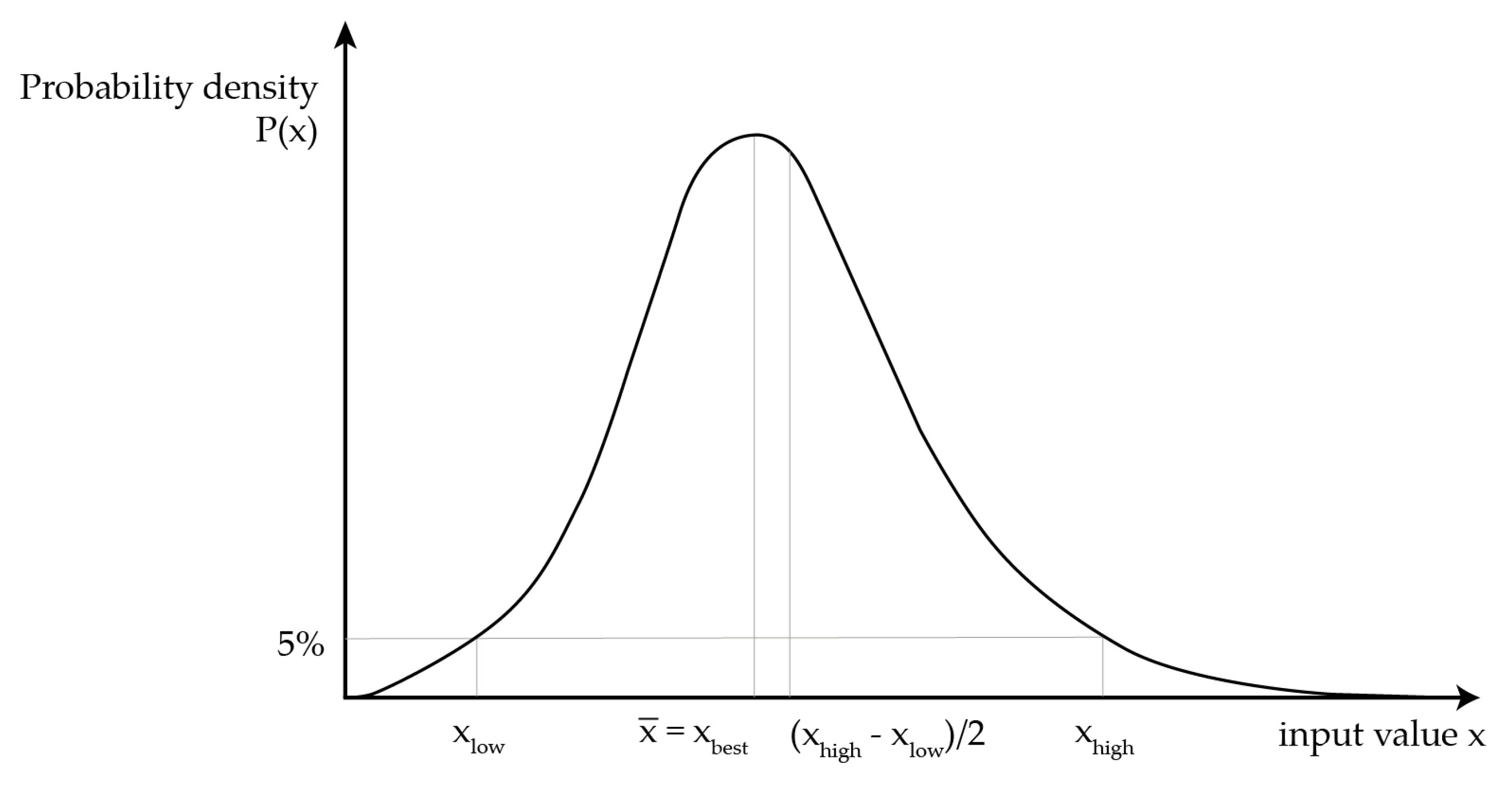
- the reasonable best estimate, xbest, and the reasonable low estimate, xlow, and the reasonable best estimate, xbest, and the samples from skewed normal distributions, x, built assuming the high and low estimates, xhigh and xlow, encompassed the 95% confidence interval and the best estimate, xbest, was the mean value (). Figure 1 shows the probability density function of a skewed normal distribution, P(x), that was built using the best, xbest, low, xlow, and high, xhigh, estimates of the input value x. This is a right-skewed distribution because it has a longer tail on the left.
The reasonable low and high estimates were determined for each model input variable to investigate how sensitive the initial ranking, i.e., ranking using the best estimates for all inputs, was to the extreme yet plausible values. Monte Carlo sampling from skewed normal distributions developed by considering the best, low and high estimates for each input was used to investigate how sensitive the initial ranking was to if the inputs are aligned to normal distributions. The more sensitive the initial ranking was to the use of different input estimates, the more significant this input uncertainty is.
The net benefit of executing a risk-reducing intervention on each asset was estimated. The risk-reducing intervention considered for all the asset is the renewal, which results in the greatest possible elimination of risk. The assets were prioritized for risk-reducing interventions in the upcoming intervention-planning period based on the net benefit of renewing them. Net benefit, nb, was defined as the difference between the reduction in risk achieved within the planning period by, and the costs and effects on rail service of executing the risk-reducing intervention. This method was used in [78] to compare intervention strategies for different railway assets, and it is based on balancing the costs and benefits of interventions [79,80,81]. The net benefit was calculated using Equation (1)
where nbk,a is the net-benefit of executing the risk-reducing intervention k on asset a; ra\k is the risk related to asset a without the execution of the intervention k; ra|k is the risk related to asset a after the execution of the intervention k; and ck,a is the costs and effects on service resulting from the execution of the intervention k. The net benefit of an asset was the difference between the reduction in risk achieved by, and the costs of, renewing the asset to a like-new state.
As one risk-reducing intervention was examined for each asset, the higher the net benefit of this intervention, the higher the asset was ranked. The set of assets a = {a1, …, aA} was converted to ranks W = {1, …, A} in descending order of the net-benefit, NBa, of restoring them where W(ia) denotes that asset a takes the position i in the W rank.
The use of each of the different input estimates—i.e., best, low, high or a value from the skewed normal distribution—resulted in a different ranking. The sensitivity of the initial ranking, i.e., ranking using the best estimates for all inputs, was evaluated by comparing it to the rankings using the low estimate, high estimate, and an estimate from the distribution. To compare the rankings, two metrics were used: (i) the cumulative number of position changes, i.e., Spearman’s rank coefficient, and (ii) weighted cumulative number of position changes, i.e., Spearman’s rank coefficient with position weights.
The cumulative number of position changes was calculated using Equation (2)
where SFX is the sum of position changes for all the assets between the ranking from the estimation of the net benefit for each asset using the best estimates for all the inputs, Wbest, and the ranking from the estimation of the net benefit for each asset using either the low or high estimate or the distribution of the estimates of the model input X and the best estimates for the rest of the inputs, WX.
As this metric does not account for the location of the changes in the list, the Spearman’s rank coefficient [82] with position weights was also used to differentiate from changes occurring in the higher positions of the rank from changes occurring in the lower positions. This method is described in [83], and the Spearman’s rank coefficient is calculated by Equation (3)
where SFX|θ is the weighted difference between the ranking Wbest, and the ranking WX, and is the average position weight of changing the position of the asset a. It was calculated using Equation (4)
where and is the position and the position weight θ of asset a, according to the ranking Wbest and and is the position and the position weight θ of asset a, according to the ranking WX. The position weights were calculated by Equation (5)
where δ is the weight of changing asset a in position Wi-1 with an asset in position Wi, nba|best is the net benefit of executing the on asset a and max(NBbest) and min(NBbest) are the highest and lowest net benefit among all the assets, calculated using the best estimates for all the inputs. Note that by using this position weight, the position changes are weighted according to the net benefit estimated using the best estimates of all input values.
Table 1, Table 2 and Table 3 presents an example comparison of only the high estimates of two model inputs for four assets, a1–a4, using the two metrics, i.e., the cumulative number of position changes, SFX, and the weighted cumulative number of position changes, SFX|θ. The use of the high estimate, instead of the best estimate, for each value results in the inversion of two assets in the ranking W. The two inputs are associated with equal SFX. This metric indicates that the uncertainty in the upwards direction for both inputs is equally important in the identification of the assets for which it is beneficial to plan a risk-reducing intervention. The high estimate of X1, however, results in an inversion on the two first positions of the ranking (Table 1 and Table 2), while the high estimate of X2 results in an inversion on the two last positions of the ranking (Table 1 and Table 3), resulting in SFx1.high|θ being higher (2) than SFx2.high|θ (1.11). This second metric indicates that the uncertainty in the upwards direction for X1 results in more significant changes in the ranking of the assets compared to the X2.
3. Case Study
3.1. Assets and Hazards
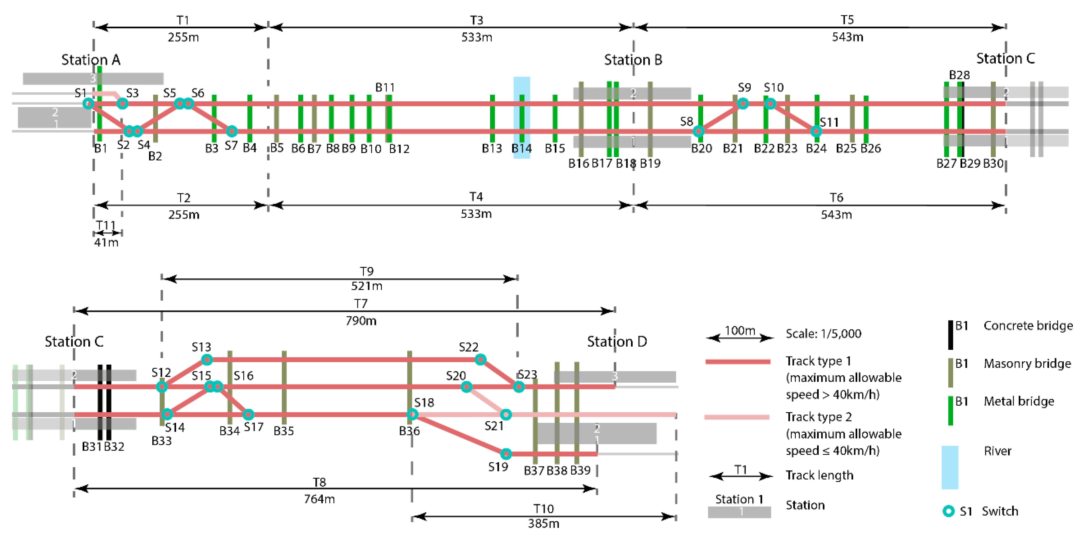
The track sections, switches, and bridges used in this case study belong to the part of the Irish railway network (Figure 2), which connects four stations, and serves both intercity and urban commuter passenger trains [84]. It consists of 11 track sections of 5 km total length and 23 switches. As the rail line crosses the city of Dublin at this part of the network, the railway is elevated above the ground level and is built on 39 bridges, which have 17,000 m2 of combined deck surface area.
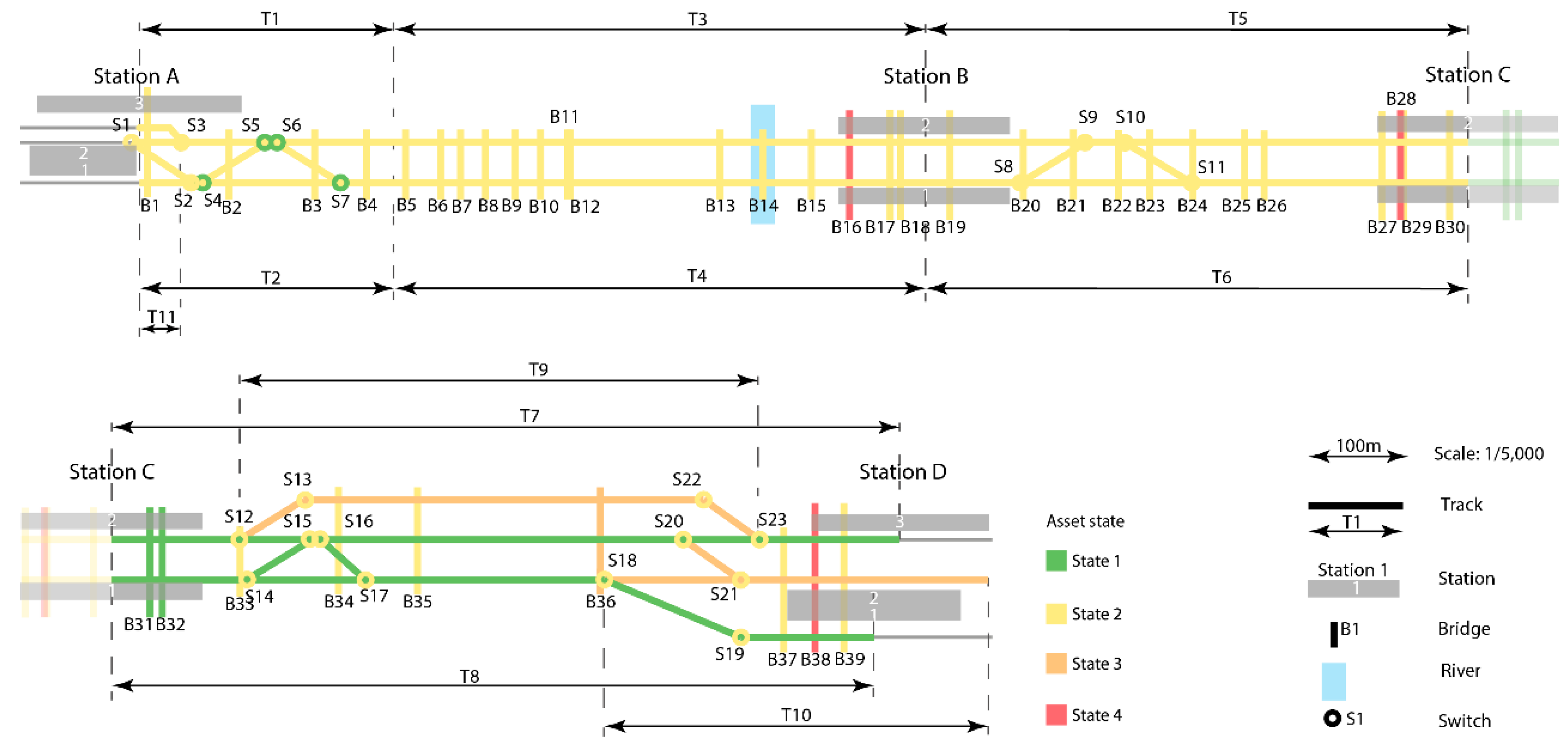
The track sections are classified into two subcategories, i.e., those with a maximum allowable speed greater than 40 km/h, and those with a maximum allowable speed lower than or equal to 40 km/h. The bridges are classified into three subcategories, i.e., concrete, masonry, and metal bridges. Each asset is considered to be in one of four possible states:
- like-new,
- slightly deteriorated,
- significantly deteriorated, and
- severely deteriorated
The states of the assets are shown in Figure 3. It is assumed that trains can operate according to the timetable in all four of these states, but that there is a probability of failure associated with each of these states. The hazards that can affect the assets were excessive traffic tonnage and two natural hazards:
- extreme heat affecting the track sections and switches, and
- river flooding affecting the bridge B14 (see Figure 2)
3.2. Risks
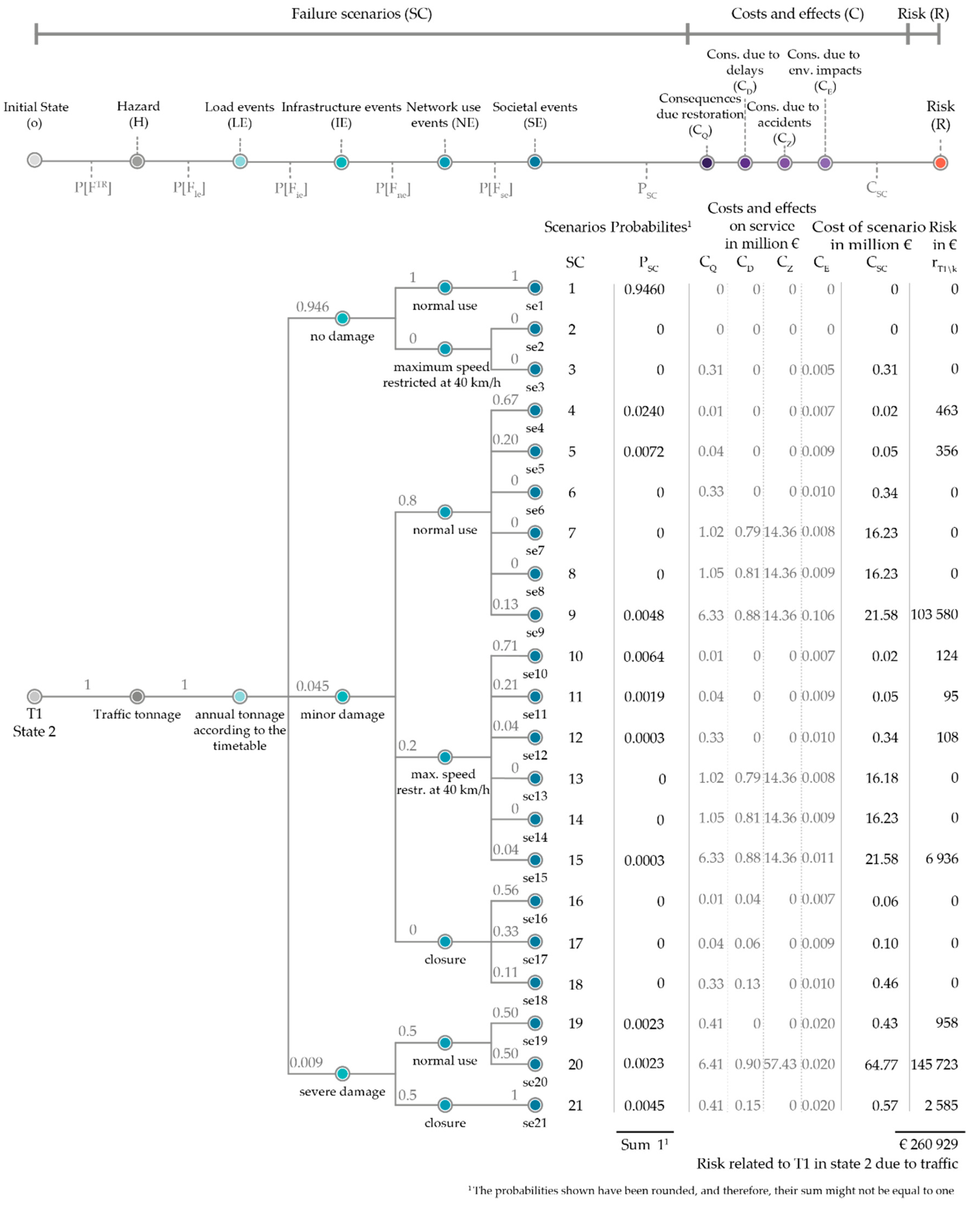
The risks, R, in the upcoming intervention-planning period were calculated as the probability of failure, P, multiplied with the consequences of failure, CF (Equation (6)), according to [85]. They were estimated using event trees [86] comprised of load, infrastructure, network use and societal events (Table 4). Different event trees were used for the estimation of risks related to each hazard type, i.e., traffic tonnage, extreme heat, and river flooding. As an example, the event tree used to estimate the risks related to track section T1 due to traffic tonnage is shown in Figure 4. The methodology used to develop the event trees can be found in [87]. Each branch of the event tree models a failure scenario, SC. The probability of occurrence of one branch of the event tree was calculated as a result of societal events Fse, network use events Fne, infrastructure events Fie, and load events Fle, using Equation (7) (Figure 4). The probability of cascading or multiple simultaneous failures were not considered. This simplification might yield either an underestimation or an overestimation of the risks [88]; however, as a railway manager in this situation dealing with such approximations, it is warranted. The risk, r, is calculated, as shown in Equation (8)
where P[FSC] is the probability of a failure scenario SC, due to traffic, TR, or due to the natural hazard, NH, i.e., extreme heat for track sections and switches or river flooding for bridge B14, and CF|SC, is the consequences, i.e., costs and effects on service, due to the failure scenario, SC.
The consequences, i.e., costs and effects on service, of a failure scenario csc were calculated for each failure scenario using Equation (9).
where cQ is the cost of restoration (Equation (10)), cD is the additional travel time cost for the passengers (Equation (11)), cZ is the cost for fatalities and injuries due to accidents (Equation (12)), and cE is the cost of environmental impacts (Equation (13)).
where CQ,a is the cost of restorations due to failure of asset a of type g. It depends on the extent of the asset l; the unit costs cQI of executing restoration interventions of type QI on asset a; and the costs CQS of site restoration works QS after the failure of the asset.
where CD,a is the cost due to additional travel time D caused by the unavailability of asset a. An asset can be unavailable due to one of two types of traffic restrictions, (1) limiting the maximum speed at 40 km/h and (2) closing the section to traffic entirely. When a traffic restriction must be applied due to the asset’s failure, it affects the entire block section where the asset is located. The effects on passengers due to the additional travel time depend on the type and duration of traffic restrictions and the total additional travel time caused when the traffic is disrupted on the block section where the asset is located. These depend on the extent of the asset l; a vector of durations of each traffic restriction type DDQI due to the execution of restoration intervention QI; a vector of durations of each traffic restriction type DDQS due to the site restoration QS; a vector of the additional travel time in minutes per traffic restriction type DT; and the unit cost of time ut.
where CZ,a is the effects due to fatalities and injuries Z incurring after accidents caused by the failure of asset a. It depends on a vector of the expected number of fatalities and injuries occurring due to accidents on the site QS caused by the failure of the asset a; and a vector of the socioeconomic costs per injury and fatality Uz.
where CE,a is the effects due to environmental impacts E caused by the execution of interventions and restorations on the site. It depends on the length of the asset used for the estimation of the environmental impacts lE; the unit cost cE|QI of the environmental impact of executing restoration intervention QI; and the cost cE|r of the environmental impact of site restoration QS after the failure of the asset. The same environmental impacts were assumed for all the interventions and restorations of the same type and all assets of the same type g.
3.3. Costs and Effects on Service of Risk-Reducing Interventions
The costs and effects on service of executing risk-reducing interventions considered were intervention costs, and the effects due to additional travel time, accidents, and environmental impacts. These are the same costs and effects on service considered for risks. They were calculated using Equations (14)–(18). In their estimation, it was assumed that:
- no damages occur on the site due to the execution of the risk-reducing interventions,
- no accidents occur due to the execution of the risk-reducing interventions, and
- the risk-reducing interventions are executed with the least possible traffic restrictions.
3.4. Variables
An overview of the variables required to estimate the net-benefit used to rank the assets for risk-reducing interventions and how they are related is given in Figure 5. An example of how Figure 5 can be read is as follows: the probability of load events is estimated as a function of the state of the asset before and after a risk-reducing intervention is executed, o\k and o|k respectively, a given amount of traffic TR or a natural hazard NH, and the type of asset g. It affects the estimation of the probability of a failure scenario P[FSC], which in turn affects the estimation of risks with ro\k and without a risk-reducing intervention ro|k, and consequently the net benefit nbk. This set-up allows updating the input values used to represent the uncertain variables when new data is collected, and, therefore also updating the net benefit related to the renewal of each asset and the ranking of the assets. This is essential, as the purpose of this analysis is to identify the input variables for which more accurate estimates must be collected to reduce the uncertainty in the ranking of the assets.
For each input uncertainty, three types of estimates were determined:
- the best estimate
- the reasonable low estimate, and
- the reasonable high estimate.
These estimates were derived from the input of experts from Irish Rail and the partners in the EU Horizon 2020 founded project DESTination RAIL, which developed a decision support tool to facilitate railway managers in intervention planning. The experts based their estimates for the assets in the case study on existing models and historical data. The analyses of the experts are described in [89,90,91,92,93]. A sample of these estimates is given in Table 5 and Table 6. The complete dataset can be found in the Supplementary File. These input values are meant to illustrate the estimation of the net benefit only for the assets of this case study and purposes of this work. The input values used in this case study might be different in other parts of the railway network in the Republic of Ireland. Further explanations on the estimation of risks related to the assets of this network can be found in [87] and [92], and on the estimation of costs and effects on service due interventions on these assets can be found in [78]. It was considered that the methods and models used to estimate the input values, as well as the risks, costs and effects on service are validated for prioritizing these assets for renewal because the scope of this analysis is to examine the effect of the input uncertainties. Hence, the effect of other uncertainties, e.g., in the models used to estimate the input values or risks, was not considered. Information on existing models and data to estimate such values can be found in the scientific literature, e.g., [1,94,95,96,97].
3.5. Results
3.5.1. Initial Ranking Using Best Estimates
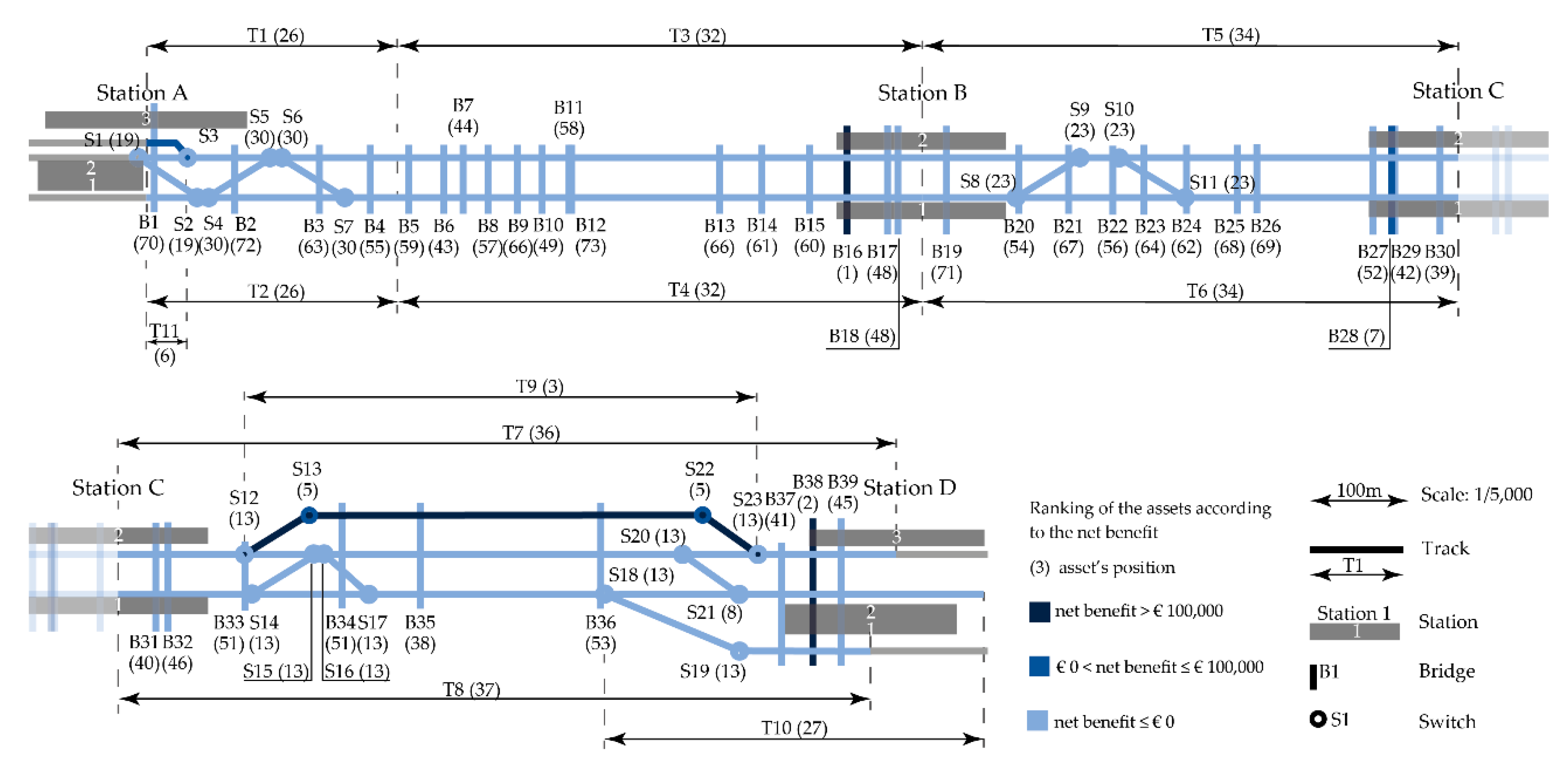
The net benefit and rank of the assets for possible risk-reducing interventions using the best estimates of the uncertain variables are shown in Figure 6. The assets were ranked from 1 to 73, and assets with the same net benefit were given the same position. The three assets with the highest net benefit were B16, B38, and T9. The net benefit of executing a risk-reduction intervention on each of these assets in the upcoming intervention-planning period was above €100,000, compared to postponing them until the next planning period. The next four assets with positive net benefit were S13, S22, T11, and B28. A risk-reducing intervention on these seven assets in the next intervention-planning period using the best estimates was beneficial because the costs and effects on service due to their renewal were less than the reduction in risk achieved by renewing them.
The remainder of the assets are switches, track sections, and bridges with a negative net benefit. If these assets were to be renewed in the upcoming intervention-planning period, the achieved reduction in risk in that period would be less than the costs and effects on service occurring due to their renewal. This certainly does not mean that it is not worthwhile to execute the risk-reducing intervention, which can only be said when the asset life-cycle costs are also evaluated. This analysis simply indicates that as regards the consequences of their renewal, there would not be a significant reduction in the risk related to these assets if they were to be renewed during the upcoming intervention-planning period.
3.5.2. Effect of Input Variable Uncertainties on Asset Rank
The effect of the input uncertainties on asset rank is presented in Table 7 and Table 8 for each uncertain variable. It can be read as follows: the low estimates of the probabilities of occurrence of load events resulted in eight position changes when no position weights were considered. They resulted in 12 position changes when position weights were considered. Contrarily, the high estimates resulted in no position changes. The use of Monte Carlo sampling from skewed normal distributions resulted in a mean of two-position changes when no position weights were considered. However, when position weights were considered, it resulted not only in a mean of five-position changes.
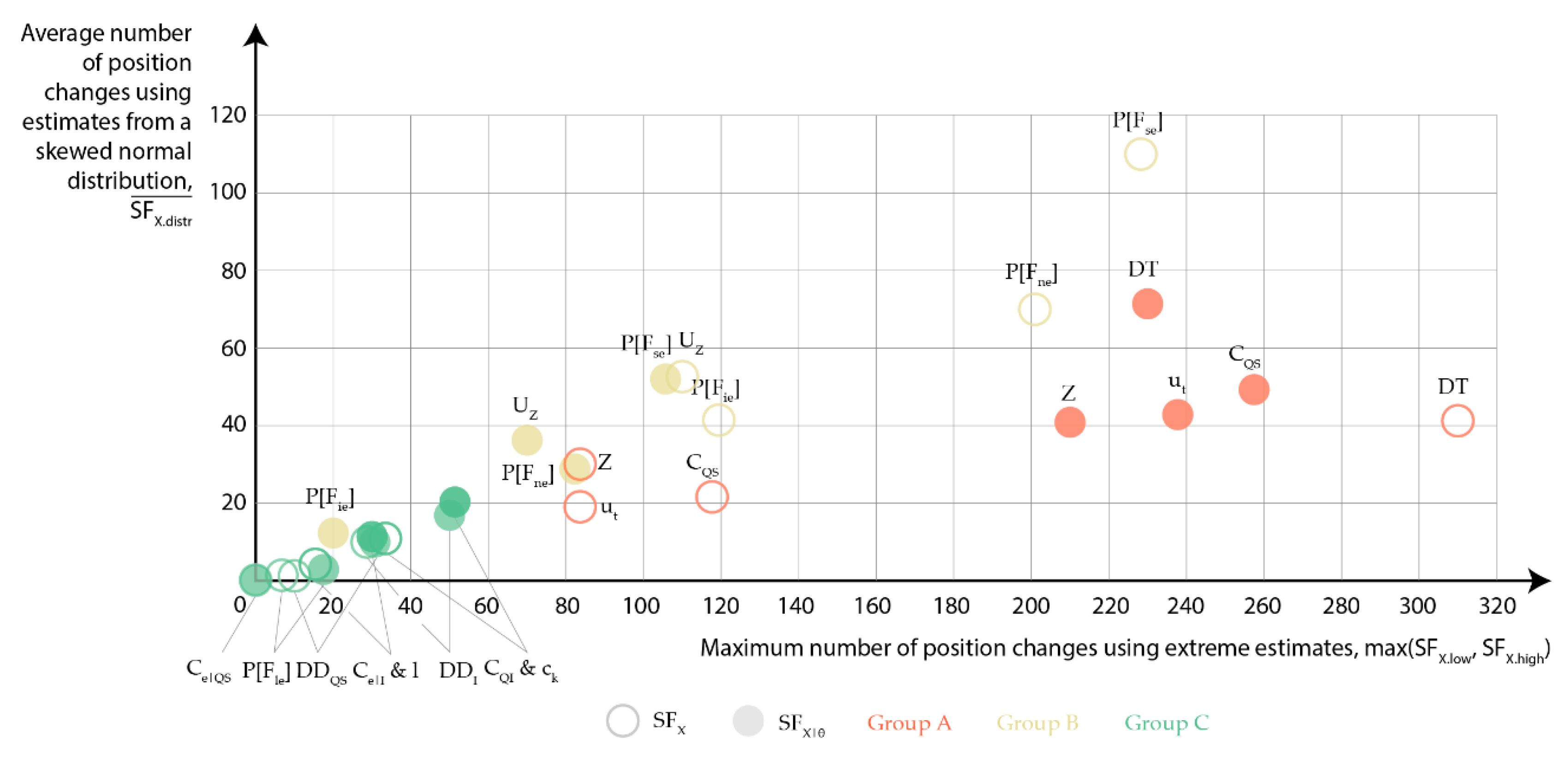
These results can be used to identify the influencing input variables whose uncertainty affects the ranking of the assets significantly. The results presented in Table 7 can be interpreted more easily by focusing on the maximum number of position changes only when the extreme estimates were used, and on the average number of position changes only when estimates from the distributions were used. This relationship is illustrated in Figure 7 with two circles for each variable: an empty circle when the position weights were not considered, SFX, and a filled circle when the position weights were considered, SFX|θ. The input variables in Figure 7 are grouped as a function of the influence of their uncertainty in the ranking of the assets:
- Group A consists of input variables where the use of extreme values and value distributions resulted in a high number of weighted position changes, i.e., the highest-ranked assets are likely to change if the input uncertainties associated with these variables are considered.
- Group B consists of input variables where the use of extreme values and distributions of values resulted in a high number of position changes but with a low number of weight position changes, i.e., the rank of the lowest-ranked assets is likely to change if the input uncertainties associated with these variables are reduced. However, this does not occur in the rank of the highest-ranked assets. The effect of these input uncertainties is more prominent when low or high values are considered than when distributions of values are considered.
- Group C consists of input variables where the use of extreme values and distributions of values resulted in very few changes to the ranking. Considering the input uncertainties associated with these variables is unlikely to change the ranking of assets; therefore, the use of best estimates is sufficient in order to prioritize the assets for risk-reducing interventions accurately.
The most influencing input variables belong to Group A. The uncertainties in the values of these inputs were found to have the greatest effect on the highest-ranked assets. These input variables are the ‘additional travel time’ DT, the ‘cost of site restoration’ CQS, the ‘unit cost of time’ ut, and the ‘number of fatalities and injuries’ Z. They are all indicated in Figure 7 with red circles.
These results prompt the following question: does the sensitivity of the ranking depend on the range of plausible values considered for each input variable? To answer this question, we examined if all the variables with the highest variance were also the most influencing ones. The variance of each input variable was considered equal to the average variance of all the skewed normal distributions used for this variable in the Monte Carlo sampling. The five input variables with the greatest variance were the ‘duration of traffic restriction due to site restoration’ DTQS, the ‘number of fatalities and injuries’ Z, the ‘probabilities of load events’ P[Fle], the ‘extent of the assets’ l and the ‘duration of traffic restriction due to interventions’ DDI. Out of these five variables, only one is in Group A: the ‘number of fatalities and injuries’ Z. The remaining four variables are in Group C. These results indicate that it is not necessarily the greatest input uncertainties that yield the greatest changes in the ranking of the assets.
Identifying the most influencing variables is often not enough to limit the input uncertainties that must be quantified to a manageable amount. This is because an input variable might take different values depending on different parameters. For example, in the case study, the input variable ‘additional travel time’ takes different values for each asset and traffic restriction type, as shown in Figure 5. Hence, to quantify the uncertainties associated with this input variable, the uncertainties in the value ‘additional travel time’ for each asset and traffic restriction type must be quantified. In this case, it is useful to identify the assets, whose rank is affected significantly when there is uncertainty in the values used to represent the ‘additional travel time’. This helps the railway manager focus on quantifying the input uncertainties of a variable only when they affect the ranking significantly. In situations when the input uncertainties of a variable do not affect the ranking of the assets, the railway manager can save resources by using the best estimates.
To identify the assets, whose rank is sensitive to the uncertainties in the variable ‘additional travel time’, we examined first how the use of samples from skewed normal distributions for this variable affects the rank of each asset. Then, we examined how many positions each asset changes in the ranking when skewed normal distributions for this variable are considered.
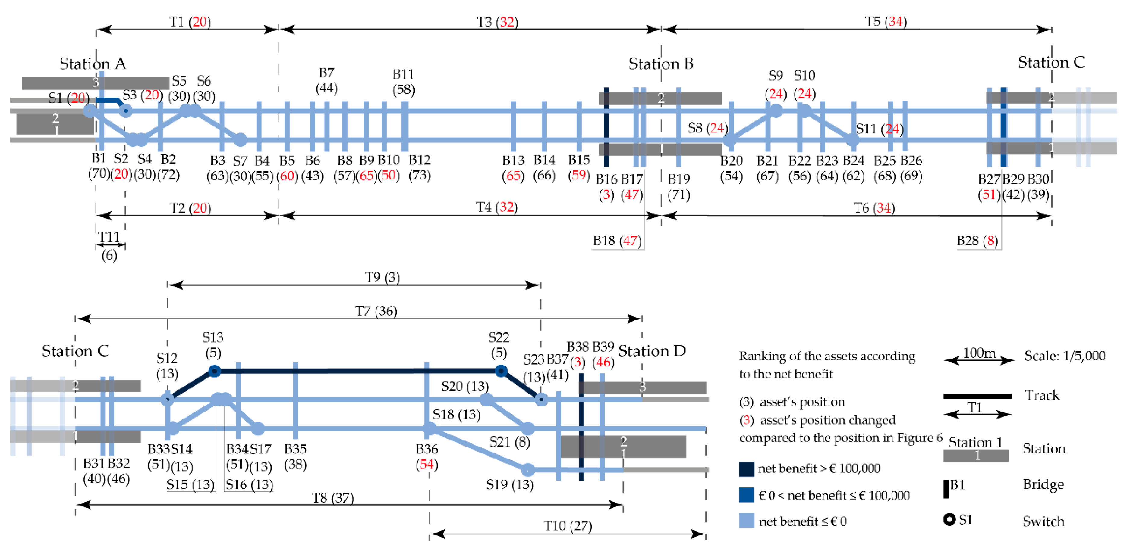
Figure 8 shows the average rank of each asset when samples of the skewed normal distributions for the variable ‘additional travel time’ and the best estimates of the rest of the variables were used. When this ranking is compared to the initial ranking (Figure 6), it can be seen that:
- 24 assets change their rank
- the first three assets with net benefit above €100,000, namely the bridges B16 and B38 and the track section T9, maintain their rank
- there are no changes in the rank of the assets with a positive net benefit
- track sections T1 and T2 have, on average, the most significant change in the ranking (6 positions).
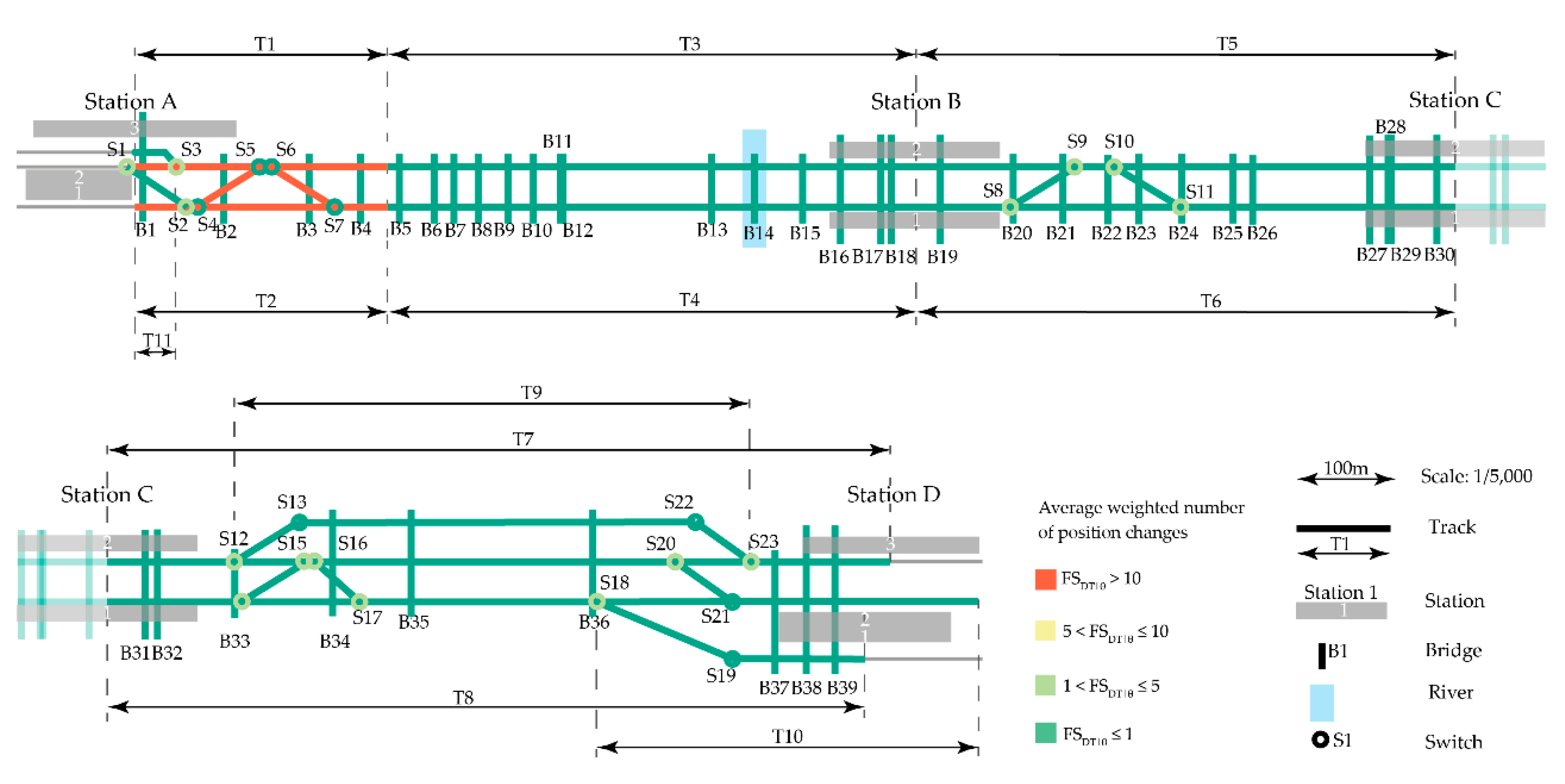
The results shown in Figure 8 indicate that the additional travel time uncertainties affect the rank of certain assets more than others. To identify the assets whose rank is affected by the additional travel time uncertainties, we examined how many positions each asset changed in the rank when samples of skewed normal distributions were used instead of best estimates for this input variable. Figure 9 shows these results. It can be seen that:
- assets T1 and T2 have the largest number of changes in rank (more than 10 positions)
- 15 switches change between one and five positions
- 56 assets change one position or less in the rank.
The results shown in Figure 9 indicate that the additional travel time uncertainties affect the rank of track sections T1 and T2 significantly. However, this uncertainty is not expected to be important in order to obtain the rank of the rest of the assets accurately. This means that quantifying the uncertainties in the values used to represent the additional travel time only for two assets might be enough to accurately identify which assets should be prioritized in this case study for risk-reducing interventions.
One possible way to quantify these input uncertainties is to use sophisticated calibrated models to determine the distribution of this value, e.g., a microscopic traffic model, like the one presented in [93]. This model uses Kronecker Algebra to estimate with high accuracy the train runs and the additional travel time caused by closures or speed restrictions due to asset unavailability. For the rest of the assets, the use of the best estimates to model the additional travel time, when they are unavailable, should be sufficient to decide whether or not they should be prioritized for interventions.
4. Discussion
This section presents how the results can be interpreted to evaluate the effect of input uncertainties and how the methodology used in this paper compares to previous studies. The implications and limitations of the presented work are also discussed, while future research directions are mentioned at the end of the section.
The results show that railway managers can identify which input uncertainties are worth quantifying by examining if the assets are prioritized differently for risk-reducing interventions when, in addition to best estimates, extreme input values and skewed normal distributions of inputs are used. This analysis offers essential information to the railway manager who wants to quantify the uncertainty when prioritizing risk-reducing interventions using best estimates of inputs. The implications of the analysis presented in this work are discussed in this section.
In this analysis, the best, low, and high estimates were determined by experts using existing models and historical data. Although data-based methods should be preferred over experts’ estimates when determining the inputs, in reality, it is often necessary to incorporate expert knowledge and experience to obtain initial results, due to data and budget constraints. This is related to a significant drawback. The input estimates might vary depending on the expert’s experience, resources, and other factors [98], which cause uncertainty in the inputs. This paper does not address the challenges obtaining input estimates from experts. Examples of such methods to are described in [39,58,99]. This paper focuses on identifying the input uncertainties that significantly affect intervention planning, regardless of the cause of uncertainty in the input estimates. The results, therefore, can only be used to identify the influencing inputs, for which the uncertainties and their sources must be identified and assessed.
Monte Carlo sampling from skewed normal distributions was used as part of the methodology to identify the input uncertainties that affect which assets are prioritized for risk-reducing interventions. Although other distributions could be used for the input variables, the use of skewed normal distributions as shown in [57,61,62,63,64,65,66], is a reasonable simplification in this analysis. This is because its scope was not to quantify the uncertainty in the ranking but to obtain an initial impression of the effect on the ranking when distribution functions of the inputs are used instead of best estimates.
There are several implications and limitations related to the methodology and results presented in this paper to discuss. By evaluating the effect of varying one input at the time, while for the rest the best estimates were used, the uncertainties in the input variables were considered to be independent. Although investigating the correlation between inputs (for example, as done in [57]) would yield a more accurate evaluation of the input uncertainties, it would also require more data and more sophisticated modeling. This would require a more resource-demanding analysis. Once initial impressions of the sensitivity of the ranking to the different input uncertainties are obtained with the analysis presented here, the railway manager knows if certain input uncertainties are likely to affect the ranking significantly. If these highly influencing input uncertainties are also likely to be correlated, the railway manager can decide to invest in determining their correlation using precise modeling.
The results provide a clear indication of which input uncertainties are likely to affect the prioritization of assets for risk-reducing interventions. These results, however, do not provide any indication of the resources required to quantify these input uncertainties and to consider them in the estimation of risks, costs and effects on service. Assessing these resources should be the next step, in order to decide which input uncertainties are worth quantifying.
The assets in the case study were prioritized based on the reduction in risk achieved after being renewed, given the costs and effects on the service of this intervention. In this case, the renewal of the assets was used as an indication of how beneficial it is to execute a risk-reducing intervention on each asset. This is a simplification, as in reality, renewing an asset is not the only way to reduce its risk. However, this simplification is justified by the scope of this analysis, which is to identify the most influencing input uncertainties when prioritizing assets for risk-reducing interventions at a high level.
The methodology presented in this paper allows railway managers to consider the input uncertainties that affect which assets are prioritized for risk-reducing interventions. To this end, risks due to asset failures—as well as the costs and effects on service due to interventions—were estimated for different railway assets at a high level. Other researchers have focused on improving the understanding and modeling of one of those factors—i.e., risks, costs and effects on service—and for specific asset types. For example, [3] presents a detailed model that simulates the causal chain from climate change to scour risk related to the bridges of Network Rail. A detailed model to estimate risks related to railway accidents, when considering different environmental conditions is presented in [100]. A detailed model to estimate and minimize passenger delays due to train delays is presented in [38]. If desired, such detailed models could be used to improve the estimates of risks, costs, and effects on service. However, often the computational effort and cost are prohibitive for large asset portfolios. Thus, this approach is taken to enable railway managers to identify the influencing uncertainties at a high level first. Then they can decide where to invest resources to improve the estimates of risks, costs, and effects on service using more detailed approaches.
Future work in this area should investigate how reliable estimates of the input variables can be obtained from experts when resource limitations do not allow to use data-based methods and how the correlation of uncertainties of these estimates can be considered. The effect of using different distribution types to model the input uncertainties should also be examined. Additionally, future work should also address the ease of reducing the input uncertainties for each variable. Finally, the complexity of planning risk-reducing interventions should be integrated by considering, for example, different intervention types for each asset and the effects on service when interventions are executed simultaneously, which is now becoming possible to analyze using the model presented by [41] or others.
5. Conclusions
This paper shows how the input uncertainties that significantly affect the assets prioritized for risk-reducing interventions were identified. It was achieved by using reasonable low and high input estimates, as well as samples from skewed normal distributions in addition to the best estimates. This approach is suitable for railway managers who have already obtained initial impressions of which assets should be prioritized for risk-reducing interventions using best estimates of the input values and who would then like to know which input uncertainties are likely to influence these results, and therefore must be quantified.
This approach was implemented on a case study to prioritize track sections, switches, and bridges for renewal. The results indicate the input variables that are related to highly influencing uncertainties. Efforts should be focused to quantify these uncertainties and efficiently improve the planning of risk-reducing interventions.
Supplementary Materials
The following are available online at https://0-www-mdpi-com.brum.beds.ac.uk/2673-4109/1/2/8/s1, A supplementary file with the input values is submitted with the paper.
Author Contributions
Conceptualization, N.P. and B.T.A.; Methodology, N.P.; Software, N.P.; Formal analysis, N.P.; Resources, N.P.; Data curation, N.P.; Writing—Original draft preparation, N.P.; Writing—Review and editing, N.P. and B.T.A.; Visualization, N.P.; Supervision, B.T.A. All authors have read and agreed to the published version of the manuscript.
Funding
The work presented here has received funding from Horizon 2020, the EU’s Framework Program for Research and Innovation for the DESTination RAIL project under grant agreement no. 636285 and for the FORESEE project under grant agreement no. 769373.
Conflicts of Interest
The authors declare that the research was conducted in the absence of any commercial or financial relationships that could be construed as a potential conflict of interest. The funders had no role in the design of the study; in the collection, analyses, or interpretation of data; in the writing of the manuscript, or in the decision to publish the results.
Appendix A
Table A1, Table A2 and Table A3 present the load, infrastructure, and network use events, respectively, per asset type. The societal events for track sections are given in Table A4 and Table A5, while Table A6 and Table A7 present the societal events for switches and bridges, respectively.

Table A1.
Load events, LE, per asset type.
| Load Event Type | Notation | Description | ||
|---|---|---|---|---|
| Track | Switches | Bridges | ||
| Traffic load | le|TR | Annual tonnage on the track section based on the timetable | Annual wheel load on the switches due to train movements based on the timetable | Normalized annual traffic loads due to the daily traffic based on the timetable |
| Level 1 load due to natural hazard | le1|NH | Thermal stresses on the track section caused by 17 °C ambient temperature | Neglectable thermal stresses on the switch elements | Neglectable increase in river flow speed |
| Level 2 load due to natural hazard | le2|NH | Thermal stresses on the track section caused by 25 °C ambient temperature | Moderate thermal stresses on the switch elements | River flow speed that corresponds to a 25-year flood event |
| Level 3 load due to natural hazard | le3|NH | Thermal stresses on the track section caused by 40 °C ambient temperature | High thermal stresses on the switch elements | River flow speed that corresponds to a 50-year flood event |
| Level 4 load due to natural hazard | le4|NH | Thermal stresses on the track section caused by 43 °C ambient temperature | Thermal stresses beyond the designed level on switch elements | River flow speed that corresponds to a 100-year flood event |
| Level 4 load due to natural hazard | le5|NH | Thermal stresses on the track section caused by 60 °C ambient temperature | - | - |
Table A2.
Infrastructure events, IE per asset type.
| Infrastructure Event Type | Notation | Description | ||
|---|---|---|---|---|
| Track | Switches | Bridges | ||
| No damage | ie1 | No noticeable damages on the track section due to the load event | No noticeable damages on the switch due to the load event | No noticeable damages on the bridge due to the load event |
| Minor damage | ie2 | Damages that partially affect the track geometry or the rail condition | Damages that partially affect either the condition of the elements or the operation of the switch | Damages that partially affect the structural stability |
| Severe damage | ie3 | Potential lack of stability of the track section to support the dynamic wheel load according to the required speed | Damages that significantly affect either the condition of the elements or the operation of the switch | Potential lack of structural stability |
Table A3.
Network use events, NE, per asset type.
| Network Use Event Type | Notation | Description | ||
|---|---|---|---|---|
| Track | Switches | Bridges | ||
| Normal use | ne1 | Fully operational track section | Fully operational block | Fully operational block |
| Maximum speed restriction | ne2 | The operation of the track section is possible only when the speed is less than 40 km/h | The operation of all affected blocks is possible only with speed below 40 km/h | The operation of the block where the bridge is located is possible only with speed below 40 km/h |
| Closure | ne3 | Closure of track section and all the blocks located in this track section | Closure of switch and all the affected blocks | Closure of the bridge and all the affected blocks |
Table A4.
Societal events, SE, used for the estimation of risk related to track sections (first part se1–se14).
Table A4.
Societal events, SE, used for the estimation of risk related to track sections (first part se1–se14).
| Notation | Description | Notation | Description |
|---|---|---|---|
| se1 | No accident; no restoration at the site and no intervention; no traffic restriction | se8 | Accident; minor restoration at the site, rail replacement and tamping of the track section; traffic restrictions due to restoration, rail replacement, and tamping |
| se2 | No accident; no restoration at the site and no intervention; maximum speed restriction for 24 hours | se9 | Accident; minor restoration at the site and renewal of the track section; traffic restrictions due to restoration and track section replacement, and maximum speed restriction for a week after renewal |
| se3 | No accident; no restoration at the site and track section renewal after a month; maximum speed for a month until track section replacement and for a week after the renewal | se10 | No accident; minor restoration at the site and tamping of the track section; maximum speed restriction until the restoration of the site is complete, and the track section is tamped |
| se4 | No accident; minor restoration at the site and tamping of the track section; traffic restrictions due to restoration and tamping | se11 | No accident; minor restoration at the site, and rail replacement and tamping of the track section; maximum speed restriction until the restoration of the site is complete, and the rail is replaced, and the track section is tamped |
| se5 | No accident; minor restoration at the site and rail replacement and tamping of the track section; traffic restrictions due to restoration and rail replacement | se12 | No accident; minor restoration at the site and track section renewal; maximum speed restriction until the restoration of the site is complete, the track is renewed and for a week after renewal |
| se6 | No accident; minor restoration at the site and renewal of the track section; traffic restrictions due to restoration and track section replacement and maximum speed restriction for a week after renewal | se13 | Accident; minor restoration at the site and tamping of the track section; maximum speed restriction until the restoration of the site is complete, and the track section is tamped |
| se7 | Accident; minor restoration at the site and tamping of the track section; traffic restrictions due to restoration and tamping | se14 | Accident; minor restoration at the site and rail replacement and tamping of the track section; maximum speed restriction until the restoration of the site is complete, the rail is replaced, and the track section is tamped |
Table A5.
Societal events, SE, used for the estimation of risk related to track sections (second part se15–se21).
Table A5.
Societal events, SE, used for the estimation of risk related to track sections (second part se15–se21).
| Notation | Description | Notation | Description |
|---|---|---|---|
| se15 | Accident; minor restoration at the site and track section renewal; maximum speed restriction until the restoration of the site is complete, the track section is renewed, and for a week after renewal | se19 | No accident; major restoration at the site and track section renewal; traffic restrictions until the restoration of the site is complete, and the track section is renewed; maximum speed restriction for a week after renewal |
| se16 | No accident; minor restoration at the site and tamping of the track section; closure of the section until the restoration of the site is complete, and the track section is tamped | se20 | Accident; major restoration at the site and track section renewal; traffic restrictions until the restoration of the site is complete, and the track section is renewed; maximum speed restriction for a week after renewal |
| se17 | No accident; minor restoration at the site, and rail replacement and tamping of the track section; closure of the section until the restoration of the site is complete, the rail is replaced and the track is tamped | se21 | No accident; major restoration at the site and track section renewal; closure of the section until the restoration of the site is complete, and the track section is renewed; maximum speed restriction for a week after renewal |
| se18 | No accident; minor restoration at the site and track section renewal; closure of the section until the restoration of the site is complete, and the track section is renewed; maximum speed restriction for a week after renewal |
Table A6.
Societal events, SE, used for the estimation of risk related to switches.
| Notation | Description | Notation | Description |
|---|---|---|---|
| se1 | No accident; no restoration at the site and no intervention; no traffic restriction | se9 | No accident; minor restoration at the site and switch renewal; maximum speed restriction until the restoration of the site is complete, and the switch is renewed |
| se2 | No accident; no restoration at the site and no intervention; maximum speed restriction for 24 hours | se10 | Accident; minor restoration at the site and welding or grinding of the switch; maximum speed restriction until the restoration of the site is complete, and welding or grinding is performed on the switch |
| se3 | No accident; no restoration at the site and switch renewal after a month; maximum speed for a month until switch renewal | se11 | Accident; minor restoration at the site and switch renewal; maximum speed restriction until the restoration of the site is complete, and the switch is renewed |
| se4 | No accident; minor restoration at the site and welding or grinding of the switch; traffic restrictions due to restoration and interventions | se12 | No accident; minor restoration at the site and welding or grinding of the switch; closure of the section until the restoration of the site is complete, and the switch is welded or ground |
| se5 | No accident; minor restoration at the site and switch renewal; traffic restrictions due to restoration and switch renewal | se13 | No accident; minor restoration at the site and switch renewal; closure of the section until the restoration of the site is complete, and the switch is renewed |
| se6 | Accident; minor restoration at the site and welding or grinding of the switch; traffic restrictions due to restoration and welding or grinding | se14 | No accident; major restoration at the site and switch renewal; traffic restrictions until the restoration of the site is complete, and the switch is renewed |
| se7 | Accident; minor restoration at the site and switch renewal; traffic restrictions due to restoration and switch renewal | se15 | Accident; major restoration at the site and switch renewal; traffic restrictions until the restoration of the site is complete, and the switch is renewed |
| se8 | No accident; minor restoration at the site and welding or grinding of the switch; maximum speed restriction until the restoration of the site is complete, and the switch is welded or ground | se16 | No accident; major restoration at the site and switch renewal; closure of the section until the restoration of the site is complete, and the switch is renewed |
Table A7.
Societal events, SE, used for the estimation of risk related to bridges.
| Notation | Description | Notation | Description |
|---|---|---|---|
| se1 | No accident; no restoration at the site and no intervention; no traffic restriction | se9 | No accident; minor restoration at the site and bridge renewal; maximum speed restriction until the restoration of the site is complete, and the bridge is renewed |
| se2 | No accident; no restoration at the site and no intervention; maximum speed restriction for 24 hours | se10 | Accident; minor restoration at the site and strengthening of the bridge; maximum speed restriction until the restoration of the site is complete, and the bridge is strengthened |
| se3 | No accident; no restoration at the site and bridge renewal after a month; maximum speed for a month until bridge renewal | se11 | Accident; minor restoration at the site and bridge renewal; maximum speed restriction until the restoration of the site is complete, and the bridge is renewed |
| se4 | No accident; minor restoration at the site and strengthening of the bridge; traffic restrictions due to restoration and interventions | se12 | No accident; minor restoration at the site and strengthening of the bridge; closure of the section until the restoration of the site is complete, and the bridge is strengthened |
| se5 | No accident; minor restoration at the site and renewal of the bridge; traffic restrictions due to restoration and bridge renewal | se13 | No accident; minor restoration at the site and bridge renewal; closure of the section until the restoration of the site is complete, and the bridge is renewed |
| se6 | Accident; minor restoration at the site and strengthening of the bridge; traffic restrictions due to restoration and intervention on the bridge | se14 | No accident; major restoration at the site and bridge renewal; traffic restrictions until the restoration of the site is complete, and the bridge is renewed |
| se7 | Accident; minor restoration at the site and renewal of the bridge; traffic restrictions due to restoration and bridge renewal | se15 | Accident; major restoration at the site and bridge renewal; traffic restrictions until the restoration of the site is complete, and the bridge is renewed |
| se8 | No accident; minor restoration at the site and strengthening of the bridge; maximum speed restriction until the restoration of the site is complete, and the bridge is strengthened | se16 | No accident; major restoration at the site and bridge renewal; closure of the section until the restoration of the site is complete, and the bridge is renewed |
References
- Koks, E.E.; Rozenberg, J.; Zorn, C.; Tariverdi, M.; Vousdoukas, M.; Fraser, S.A.; Hall, J.W.; Hallegatte, S. A global multi-hazard risk analysis of road and railway infrastructure assets. Nat. Commun. 2019, 10, 2677. [Google Scholar] [CrossRef] [Green Version]
- Macciotta, R.; Martin, C.D.; Cruden, D.M.; Hendry, M.T.; Edwards, T. Rock fall hazard control along a section of railway based on quantified risk. Georisk Assess. Manag. Risk Eng. Syst. Geohazards 2017, 11, 272–284. [Google Scholar] [CrossRef]
- Dikanski, H.; Hagen-Zanker, A.; Imam, B.; Avery, K. Climate change impacts on railway structures: Bridge scour. Proc. Inst. Civ. Eng. Eng. Sustain. 2016, 170, 237–248. [Google Scholar] [CrossRef]
- Zampieri, P.; Zanini, M.A.; Modena, C. Simplified seismic assessment of multi-span masonry arch bridges. Bull. Earthq. Eng. 2015, 13, 2629–2646. [Google Scholar] [CrossRef]
- Hong, L.; Ouyang, M.; Peeta, S.; He, X.; Yan, Y. Vulnerability assessment and mitigation for the Chinese railway system under floods. Reliab. Eng. Syst. Saf. 2015, 137, 58–68. [Google Scholar] [CrossRef]
- Chang, S.E.; Nojima, N. Measuring post-disaster transportation system performance: The 1995 Kobe earthquake in comparative perspective. Transp. Res. Part A Policy Pract. 2001, 35, 475–494. [Google Scholar] [CrossRef]
- Baker, C.J.; Cheli, F.; Orellano, A.; Paradot, N.; Proppe, C.; Rocchi, D. Cross-wind effects on road and rail vehicles. Veh. Syst. Dyn. 2009, 47, 983–1022. [Google Scholar] [CrossRef]
- Baker, C.J. A framework for the consideration of the effects of crosswinds on trains. J. Wind Eng. Ind. Aerodyn. 2013, 123, 130–142. [Google Scholar] [CrossRef]
- Arkell, B.P.; Darch, G.J.C. Impact of climate change on London’s transport network. Proc. Inst. Civ. Eng. Munic. Eng. 2006, 159, 231–237. [Google Scholar] [CrossRef]
- Lambert, J.H.; Sarda, P. Terrorism scenario identification by superposition of infrastructure networks. J. Infrastruct. Syst. 2005, 11, 211–220. [Google Scholar] [CrossRef]
- Dobney, K.; Baker, C.J.; Chapman, L.; Quinn, A.D. The future cost to the United Kingdom’s railway network of heat-related delays and buckles caused by the predicted increase in high summer temperatures owing to climate change. Proc. Inst. Mech. Eng. Part F J. Rail Rapid Transit 2010, 224, 25–34. [Google Scholar] [CrossRef]
- Argyroudis, S.; Kaynia, A.M. Analytical seismic fragility functions for highway and railway embankments and cuts. Earthq. Eng. Struct. Dyn. 2015, 44, 1863–1879. [Google Scholar] [CrossRef]
- Nielsen, J.C.O.; Li, X. Railway track geometry degradation due to differential settlement of ballast/subgrade – Numerical prediction by an iterative procedure. J. Sound Vib. 2018, 412, 441–456. [Google Scholar] [CrossRef]
- Lamb, R.; Aspinall, W.; Odbert, H.; Wagener, T. Vulnerability of bridges to scour: Insights from an international expert elicitation workshop. Nat. Hazards Earth Syst. Sci. 2017, 17, 1393–1409. [Google Scholar] [CrossRef] [Green Version]
- Jamshidi, A.; Faghih-Roohi, S.; Núñez, A.; Babuska, R.; Schutter, B.D.; Dollevoet, R.; Li, Z. Probabilistic defect-based risk assessment approach for rail failures in railway infrastructure. IFAC PapersOnLine 2016, 49, 73–77. [Google Scholar] [CrossRef]
- Ghodrati, B.; Famurewa, S.; Hoseinie, S.H. Railway switches and crossings reliability analysis. In Proceedings of the IEEE International Conference on Industrial Engineering and Engineering Management (IEEM), Bali, Indondesia, 4–7 December 2016; pp. 1412–1416. [Google Scholar]
- Pams Capoccioni, C.; Nivon, D.; Amblard, J.; De Cesare, G.; Ghilardi, T.; Jafarnejad, M.; Battisacco, E. Analysis of ballast transport in the event of overflowing of the drainage system on high speed lines. La Houille Blanche 2015, 4, 39–45. [Google Scholar] [CrossRef]
- Ferdous, W.; Manalo, A. Failures of mainline railway sleepers and suggested remedies—Review of current practice. Eng. Fail. Anal. 2014, 44, 17–35. [Google Scholar] [CrossRef]
- Remennikov, A.M.; Kaewunruen, S. Experimental load rating of aged railway concrete sleepers. Eng. Struct. 2014, 76, 147–162. [Google Scholar] [CrossRef] [Green Version]
- Zerbst, U.; Beretta, S. Failure and damage tolerance aspects of railway components. Eng. Fail. Anal. 2011, 18, 534–542. [Google Scholar] [CrossRef]
- Malm, R.; Andersson, A. Field testing and simulation of dynamic properties of a tied arch railway bridge. Eng. Struct. 2006, 28, 143–152. [Google Scholar] [CrossRef]
- Park, J.; Towashiraporn, P. Rapid seismic damage assessment of railway bridges using the response-surface statistical model. Struct. Saf. 2014, 47, 1–12. [Google Scholar] [CrossRef]
- An, M.; Huang, S.; Baker, C.J. Railway risk assessment—the fuzzy reasoning approach and fuzzy analytic hierarchy process approaches: A case study of shunting at Waterloo depot. Proc. Inst. Mech. Eng. Part F J. Rail Rapid Transit 2007, 221, 365–383. [Google Scholar] [CrossRef]
- Dick, T.C.; Barkan, C.P.L.; Chapman, E.R.; Stehly, M.P. Multivariate statistical model for predicting occurrence and location of broken rails. Transp. Res. Rec. J. Transp. Res. Board 2003, 1825, 48–55. [Google Scholar] [CrossRef] [Green Version]
- Sussmann, T.R.; Ruel, M.; Chrismer, S.M. Source of ballast fouling and influence considerations for condition assessment criteria. Transp. Res. Rec. J. Transp. Res. Board 2012, 2289, 87–94. [Google Scholar] [CrossRef]
- Holický, M.; Marková, J.; Sýkora, M. Forensic assessment of a bridge downfall using Bayesian networks. Eng. Fail. Anal. 2013, 30, 1–9. [Google Scholar] [CrossRef]
- Benn, J. Railway bridge failure during flooding in the UK and Ireland. Proc. Inst. Civ. Eng. Forensic Eng. 2013, 166, 163–170. [Google Scholar] [CrossRef]
- Liu, X.; Saat, M.R.; Barkan, C.P.L. Analysis of causes of major train derailment and their effect on accident rates. Transp. Res. Rec. J. Transp. Res. Board 2012, 2289, 154–163. [Google Scholar] [CrossRef]
- Dinh, V.N.; Kim, K.D.; Warnitchai, P. Dynamic analysis of three-dimensional bridge–high-speed train interactions using a wheel–rail contact model. Eng. Struct. 2009, 31, 3090–3106. [Google Scholar] [CrossRef]
- Barkan, C.P.L.; Dick, T.C.; Anderson, R.T. Railroad derailment factors affecting hazardous materials transportation risk. Transp. Res. Rec. J. Transp. Res. Board 2003, 1825, 64–74. [Google Scholar] [CrossRef]
- Liu, X.; Barkan, C.P.L.; Saat, M.R. Analysis of derailments by accident cause. Transp. Res. Rec. J. Transp. Res. Board 2011, 2261, 178–185. [Google Scholar] [CrossRef] [Green Version]
- Jafarian, E.; Rezvani, M.A. Application of fuzzy fault tree analysis for evaluation of railway safety risks: An evaluation of root causes for passenger train derailment. Proc. Inst. Mech. Eng. Part F J. Rail Rapid Transit 2012, 226, 14–25. [Google Scholar] [CrossRef]
- Liu, X. Statistical temporal analysis of freight train derailment rates in the United States. Transp. Res. Rec. J. Transp. Res. Board 2015, 2476, 119–125. [Google Scholar] [CrossRef]
- Liu, X.; Saat, M.R.; Barkan, C.P.L. Freight-train derailment rates for railroad safety and risk analysis. Accid. Anal. Prev. 2017, 98, 1–9. [Google Scholar] [CrossRef]
- Chen, D. Derailment risk due to coupler jack-knifing under longitudinal buff force. Proc. Inst. Mech. Eng. Part F J. Rail Rapid Transit 2010, 224, 483–490. [Google Scholar] [CrossRef]
- Evans, A.W. Estimating transport fatality risk from past accident data. Accid. Anal. Prev. 2003, 35, 459–472. [Google Scholar] [CrossRef]
- Zhao, W.; Martin, U.; Cui, Y.; Liang, J. Operational risk analysis of block sections in the railway network. J. Rail Transp. Plan. Manag. 2017, 7, 245–262. [Google Scholar]
- Corman, F. Interactions and equilibrium between rescheduling train traffic and routing passengers in microscopic delay management: A game theoretical study. Transp. Sci. 2020, 54, 785–822. [Google Scholar] [CrossRef]
- Ćirović, G.; Pamučar, D. Decision support model for prioritizing railway level crossings for safety improvements: Application of the adaptive neuro-fuzzy system. Expert Syst. Appl. 2013, 40, 2208–2223. [Google Scholar] [CrossRef]
- Morcous, G.; Lounis, Z. Maintenance optimization of infrastructure networks using genetic algorithms. Autom. Constr. 2005, 14, 129–142. [Google Scholar] [CrossRef]
- Burkhalter, M.; Adey, B.T. A Network flow model approach to determining optimal intervention programs for railway infrastructure networks. Infrastructures 2018, 3, 31. [Google Scholar] [CrossRef] [Green Version]
- Burkhalter, M.; Adey, B.T. Determining optimal intervention programs for large railway infrastructure networks using a genetic algorithm. In Proceedings of the 12th World Congress on Railway Research, Tokio, Japan, 28 October–1 November 2019. [Google Scholar]
- Guler, H. Decision support system for railway track maintenance and renewal management. J. Comput. Civ. Eng. 2013, 27, 292–306. [Google Scholar] [CrossRef]
- Gaudry, M.; Lapeyre, B.; Quinet, É. Infrastructure maintenance, regeneration and service quality economics: A rail example. Transp. Res. Part B Methodol. 2016, 86, 181–210. [Google Scholar] [CrossRef] [Green Version]
- Azad, N.; Hassini, E.; Verma, M. Disruption risk management in railroad networks: An optimization-based methodology and a case study. Transp. Res. Part B Methodol. 2016, 85, 70–88. [Google Scholar] [CrossRef]
- Jaiswal, P.; Van Westen, C.J.; Jetten, V. Quantitative assessment of landslide hazard along transportation lines using historical records. Landslides 2011, 8, 279–291. [Google Scholar] [CrossRef]
- Bemment, S.D.; Goodall, R.M.; Dixon, R.; Ward, C.P. Improving the reliability and availability of railway track switching by analysing historical failure data and introducing functionally redundant subsystems. Proc. Inst. Mech. Eng. Part F J. Rail Rapid Transit 2018, 232, 1407–1424. [Google Scholar] [CrossRef] [PubMed] [Green Version]
- Bartram, D.; Burrow, M.P.N.; Yao, X. A computational intelligence approach to railway track intervention planning. In Studies in Computational Intelligence; Yu, T., Davis, L., Baydar, C., Roy, R., Eds.; Springer: Berlin/Heidelberg, Germany, 2008; pp. 163–198. [Google Scholar]
- Jaroszweski, D.; Fu, Q.; Easton, J. A data model for heat-related rail buckling: Implications for operations, maintenance and long-term adaptation. In Proceedings of the 12th World Congress on Railway Research, Tokyo, Japan, 28 October–1 November 2019. [Google Scholar]
- Jamshidi, A.; Faghih-Roohi, S.; Hajizadeh, S.; Núñez, A.; Babuska, R.; Dollevoet, R.; Schutter, B.D. A big data analysis approach for rail failure risk assessment. Risk Anal. 2017, 37, 1495–1507. [Google Scholar] [CrossRef] [PubMed] [Green Version]
- Santamaria, J.; Vadillo, E.G.; Gomez, J. Influence of creep forces on the risk of derailment of railway vehicles. Veh. Syst. Dyn. 2009, 47, 721–752. [Google Scholar] [CrossRef] [Green Version]
- Bana e Costa, C.; Oliveira, C.; Vieira, V. Prioritization of bridges and tunnels in earthquake risk mitigation using multicriteria decision analysis: Application to Lisbon. Omega 2008, 36, 442–450. [Google Scholar] [CrossRef]
- Zhao, J.; Chan, A.H.C.; Burrow, M.P.N. Probabilistic model for predicting rail breaks and controlling risk of derailment. Transp. Res. Rec. J. Transp. Res. Board 2007, 1995, 76–83. [Google Scholar] [CrossRef]
- Podofillini, L.; Zio, E.; Vatn, J. Risk-informed optimisation of railway tracks inspection and maintenance procedures. Reliab. Eng. Syst. Saf. 2006, 91, 20–35. [Google Scholar] [CrossRef]
- Aven, T. Misconceptions of Risk; John Wiley & Sons: Chichester, UK, 2010. [Google Scholar]
- Scholten, L.; Schuwirth, N.; Reichert, P.; Lienert, J. Tackling uncertainty in multi-criteria decision analysis—An application to water supply infrastructure planning. Eur. J. Oper. Res. 2015, 242, 243–260. [Google Scholar] [CrossRef] [Green Version]
- Patra, A.P.; Söderholm, P.; Kumar, U. Uncertainty estimation in railway track life-cycle cost: A case study from Swedish National Rail Administration. Proc. Inst. Mech. Eng. Part F J. Rail Rapid Transit 2009, 223, 285–293. [Google Scholar] [CrossRef]
- Washington, S.P.; Oh, J. Bayesian methodology incorporating expert judgment for ranking countermeasure effectiveness under uncertainty: Example applied to at grade railroad crossings in Korea. Accid. Anal. Prev. 2006, 38, 234–247. [Google Scholar] [CrossRef] [PubMed]
- Wang, L.; An, M.; Qin, Y.; Jia, L.M. A risk-based maintenance decision-making approach for railway asset management. Int. J. Softw. Eng. Knowl. Eng. 2018, 28, 453–483. [Google Scholar] [CrossRef]
- Hohl, M.; Brem, S.; Balmer, J.; Schulze, T.; Holthausen, N.; Vermeulen, E.; Bohnenblust, H.; Zulauf, C. A Method for Risk Analysis of Disasters and Emergencies in Switzerland; Federal Office for Civil Protection: Bern, Switzerland, 2013. [Google Scholar]
- Braband, J.; Schäbe, H. Propagation of uncertainty in railway signaling risk analysis. In Safety and Reliability of Complex Engineered Systems; CRC Press: Zurich, Switzerland, 2015; pp. 2623–2626. [Google Scholar]
- Rama, D.; Andrews, J.D. A reliability analysis of railway switches. Proc. Inst. Mech. Eng. Part F J. Rail Rapid Transit 2013, 227, 344–363. [Google Scholar] [CrossRef]
- Quiroga, L.M.; Schnieder, E. Monte Carlo simulation of railway track geometry deterioration and restoration. Proc. Inst. Mech. Eng. Part O J. Risk Reliab. 2012, 226, 274–282. [Google Scholar] [CrossRef]
- Ghazel, M. Using stochastic petri nets for level-crossing collision risk assessment. IEEE Trans. Intell. Transp. Syst. 2009, 10, 668–677. [Google Scholar] [CrossRef]
- Macciotta, R.; Martin, C.D.; Morgenstern, N.R.; Cruden, D.M. Quantitative risk assessment of slope hazards along a section of railway in the Canadian Cordillera—A methodology considering the uncertainty in the results. Landslides 2016, 13, 115–127. [Google Scholar] [CrossRef]
- Andrews, J.D. A modelling approach to railway track asset management. Proc. Inst. Mech. Eng. Part F J. Rail Rapid Transit 2013, 227, 56–73. [Google Scholar] [CrossRef]
- Patra, A.P. Maintenance Decision Support Models for Railway Infrastructure Using RAMS & LCC Analyses. Ph.D. Thesis, Luleå University of Technology, Luleå, Sweden, 2009. [Google Scholar]
- Andrade, A.R. Renewal decisions from a Life-cycle Cost (LCC) Perspective in Railway Infrastructure: An integrative Approach Using Separate LCC Models for Rail and Ballast Components. Ph.D. Thesis, Universidade Técnica de Lisboa, Lisbon, Portugal, 2008. [Google Scholar]
- Andrews, J.D.; Prescott, D.; De Rozières, F. A stochastic model for railway track asset management. Reliab. Eng. Syst. Saf. 2014, 130, 76–84. [Google Scholar] [CrossRef]
- Feng, D.; He, Z.; Lin, S.; Wang, Z.; Sun, X. Risk index system for catenary lines of high-speed railway considering the characteristics of time–space differences. IEEE Trans. Transp. Electrif. 2017, 3, 739–749. [Google Scholar] [CrossRef]
- Qiu, S.; Sallak, M.; Schön, W.; Cherfi-Boulanger, Z. Availability assessment of railway signalling systems with uncertainty analysis using Statecharts. Simul. Model. Pract. Theory 2014, 47, 1–18. [Google Scholar] [CrossRef]
- Bickel, P.; Friedrich, R. ExternE: Externalities of Energy: Methodology 2005 Update; Office for Official Publications of the European Communities: Luxembourg, 2005. [Google Scholar]
- Wheat, P.; Smith, A.S.J.; Nash, C. CATRIN (Cost Allocation of TRansport INfrastructure cost), Deliverable 8—Rail Cost Allocation for Europe; Sixth Framework Programme: Stockholm, Sweden, 2009. [Google Scholar]
- Barker, K.; Haimes, Y.Y. Uncertainty analysis of interdependencies in dynamic infrastructure recovery: Applications in risk-based decision making. J. Infrastruct. Syst. 2009, 15, 394–405. [Google Scholar] [CrossRef]
- Cholette, M.E.; Ma, L.; Buckingham, L.; Allahmanli, L.; Bannister, A.; Xie, G. A Decision support framework for prioritization of engineering asset management activities under uncertainty. In Proceedings of the World Congress on Engineering Asset Management (WCEAM), Pretoria, South Africa, 28–31 October 2014; pp. 49–60. [Google Scholar]
- Zampetakis, L.A.; Moustakis, V.S. Quantifying uncertainty in ranking problems with composite indicators: A Bayesian approach. J. Model. Manag. 2010, 5, 63–80. [Google Scholar] [CrossRef]
- Ellis, J.; Smith, E.; Spouge, J. Research on Risk models at European Level—Final Report; Det Norske Verital Limited (DNV GL): London, UK, 2016. [Google Scholar]
- Papathanasiou, N.; Adey, B.T. Usefulness of quantifying effects on rail service when comparing intervention strategies. Infrastruct. Asset Manag. 2020, 1–20. [Google Scholar] [CrossRef] [Green Version]
- Hudson, W.; Haas, R.; Uddin, W. Infrastructure Management: Integrating Design, Construction, Maintenance, Rehabilitation, and Renovation; McGraw-Hill: New York, NY, USA, 1997. [Google Scholar]
- Adey, B.T.; Hajdin, R.; Brühwiler, E. Supply and demand system approach to development of bridge management strategies. J. Infrastruct. Syst. 2003, 9, 117–131. [Google Scholar] [CrossRef]
- Adey, B.T.; Martani, C.; Papathanasiou, N.; Burkhalter, M. Estimating and communicating the risk of neglecting maintenance. Infrastruct. Asset Manag. 2019, 6, 109–128. [Google Scholar] [CrossRef] [Green Version]
- Spearman, C. The proof and measurement of association between two things. Am. J. Psychol. 1904, 15, 72. [Google Scholar] [CrossRef]
- Kumar, R.; Vassilvitskii, S. Generalized distances between rankings. In Proceedings of the 19th International Conference on World Wide Web (WWW), New York, NY, USA, 26–30 April 2010; p. 571. [Google Scholar]
- National Transport Authority. National Heavy Rail Census; National Transport Authority: Dublin, Ireland, 2019. [Google Scholar]
- ISO. Guide 73: Risk Management—Vocabulary; ISO copyright office: Geneva, Switzerland, 2009. [Google Scholar]
- ISO. ISO 31010—Risk Management—Risk Assessment Techniques; ISO copyright office: Geneva, Switzerland, 2009. [Google Scholar]
- Papathanasiou, N.; Adey, B.T. Making comparable risk estimates for railway assets of different types. Infrastruct. Asset Manag. 2020. (under review). [Google Scholar]
- Adey, B.T.; Hajdin, R.; Brühwiler, E. Effect of common cause failures on indirect costs. J. Bridg. Eng. 2004, 9, 200–208. [Google Scholar] [CrossRef]
- Bukhsh, Z.A.; Stipanovic, I.; Connolly, L.; Adey, B.; Papathanasiou, N.; Gavin, K.; Martinovic, C.; Ramdas, V.; Barett, A.; Schoebel, A. Report on Decision Support Tool; DESTination RAIL Deliverable D3.3: Enschede, The Netherlands, 2017. [Google Scholar]
- Connolly, L.; O’Connor, A.J. Guideline for Probability Based Multi Criteria Performance Optimisation of Railway Infrastructure; DESTination RAIL Deliverable 2.1: Dublin, Ireland, 2017. [Google Scholar]
- Barrett, A.; Ramdas, V. Report on the Network Whole Cost Model; DESTination RAIL Deliverable D4.3: Wokingham, UK, 2018. [Google Scholar]
- Papathanasiou, N.; Adey, B.T.; Burkhalter, M. Risk Assessment Methodology; DESTination RAIL Deliverable D3.6: Brussels, Belgium, 2018. [Google Scholar]
- Aksentijevic, J.; Blieberger, J.; Stefan, M.; Schöbel, A. Report on Traffic Flow Model; DESTination RAIL Deliverable D4.2: Vienna, Austria, 2017. [Google Scholar]
- Stenström, C.; Norrbin, P.; Parida, A.; Kumar, U. Preventive and corrective maintenance—Cost comparison and cost–benefit analysis. Struct. Infrastruct. Eng. 2016, 12, 603–617. [Google Scholar] [CrossRef]
- Ghofrani, F.; He, Q.; Goverde, R.M.P.; Liu, X. Recent applications of big data analytics in railway transportation systems: A survey. Transp. Res. Part C Emerg. Technol. 2018, 90, 226–246. [Google Scholar] [CrossRef]
- Neuhold, J.; Landgraf, M. From data-based condition analysis to sophisticated asset management for railway tracks. In Proceedings of the 12th World Congress on Railway Research, Tokyo, Japan, 28 October–1 November 2019. [Google Scholar]
- Lu, C.-L.; Lai, Y.-C. Optimal rail system design with multiple layers of fault and event trees. J. Transp. Saf. Secur. 2019, 1–22. [Google Scholar] [CrossRef]
- Lidén, T. Railway Infrastructure Maintenance—A Survey of Planning Problems and Conducted Research. Transp. Res. Procedia 2015, 10, 574–583. [Google Scholar] [CrossRef] [Green Version]
- You, X.; Tonon, F. Event tree and fault tree analysis in tunneling with imprecise probabilities. In Proceedings of the GeoCongress, Oakland, CA, USA, 25–29 March 2012; pp. 2885–2894. [Google Scholar]
- Sadler, J.; Kit, O.; Austin, J.; Griffin, D. A tool to predict environmental risk to UK rail infrastructure. Proc. Inst. Civ. Eng. Transp. 2018, 171, 115–124. [Google Scholar] [CrossRef]
Figure 1.
Illustration of the best, low and high estimates and a right-skewed normal distribution of input value X.
Figure 1.
Illustration of the best, low and high estimates and a right-skewed normal distribution of input value X.

Figure 2.
Infrastructure assets: track sections, switches and bridges.

Figure 3.
State of assets without the execution of risk-reducing interventions, Oa\k.

Figure 4.
The event tree used to estimate the risk related to T1 due to traffic tonnage without the execution of the risk-reducing intervention (adopted from [87]). The societal events are described in Table A4 and Table A5 in the Appendix A.
Figure 4.
The event tree used to estimate the risk related to T1 due to traffic tonnage without the execution of the risk-reducing intervention (adopted from [87]). The societal events are described in Table A4 and Table A5 in the Appendix A.

Figure 5.
Overview of the variables required to estimate the net benefit.

Figure 6.
Assets ranked according to net benefit, using the best estimates for all the uncertain input variables.
Figure 6.
Assets ranked according to net benefit, using the best estimates for all the uncertain input variables.

Figure 7.
Effect of input variable uncertainties on asset rank.

Figure 8.
Assets ranked using Monte Carlo sampling from skewed normal distributions for the variable ‘additional travel time’ (DT) and the best estimates for the rest of the uncertain variables.
Figure 8.
Assets ranked using Monte Carlo sampling from skewed normal distributions for the variable ‘additional travel time’ (DT) and the best estimates for the rest of the uncertain variables.

Figure 9.
Expected number of weighted position changes using Monte Carlo sampling from skewed normal distributions for the variable ‘additional travel time’ (DT) and the best estimates for the rest of the uncertain variables.
Figure 9.
Expected number of weighted position changes using Monte Carlo sampling from skewed normal distributions for the variable ‘additional travel time’ (DT) and the best estimates for the rest of the uncertain variables.

Table 1.
Example of ranking using the best estimates of two model inputs, X1 and X2.
| Assets | Net Benefit | Rank | Weight of Position Change | Position Weight |
|---|---|---|---|---|
Equation (1) | Equation (5) | Equation (5) | ||
| a1 | 100 | 1 | 1.00 | 0.0 |
| a2 | 20 | 2 | 0.47 | 1.0 |
| a3 | 0 | 3 | 0.33 | 1.5 |
| a4 | −50 | 4 | 0.00 | 1.8 |
Table 2.
Example of ranking using the high estimate of one model input, X1.high, and the best estimate of one model input, X2.best.
Table 2.
Example of ranking using the high estimate of one model input, X1.high, and the best estimate of one model input, X2.best.
| Assets | Net Benefit | Rank | No. of Position Changes | Position Weight | No. of Weighted Position Changes |
|---|---|---|---|---|---|
Equation (1) | Equation (2) | Equation (5) | Equation (3) | ||
| a1 | 120 | 2 | 1 | 1.0 | 1.00 |
| a2 | 150 | 1 | 1 | 0.0 | 1.00 |
| a3 | 50 | 3 | 0 | 1.5 | 0.00 |
| a4 | 0 | 4 | 0 | 1.8 | 0.00 |
| Sum | 2 | 2.00 |
Table 3.
Example of ranking using the best estimate of one model input, X1.best, and the high estimate of one model input, X2.high.
Table 3.
Example of ranking using the best estimate of one model input, X1.best, and the high estimate of one model input, X2.high.
| Assets | Net Benefit | Rank | No. of Position Changes | Position Weight | No. of Weighted Position Changes |
|---|---|---|---|---|---|
Equation (1) | Equation (2) | Equation (5) | Equation (3) | ||
| a1 | 150 | 1 | 0 | 0.0 | 0.0 |
| a2 | 120 | 2 | 0 | 1.0 | 0.0 |
| a3 | 50 | 4 | 1 | 1.8 | 0.6 |
| a4 | 100 | 3 | 1 | 1.5 | 0.6 |
| Sum | 2 | 1.11 |
Table 4.
Event types.
| Type | Notation | Description | Example of Event Used in the Case Study for the Track Section T1 1 |
|---|---|---|---|
| Hazard | h | An event that may lead to a change in the load and stress level applied on a railway asset | Traffic |
| Load | le | An event that may change the load and stress levels applied on a railway asset | Annual tonnage on the track section T1 based on the timetable (1043 trains during a weekday and 318 trains during the weekend) |
| Infrastructure | ie | An event that may change the structural or functional properties of a railway asset | Damages that partially affect the geometry or the rail condition of the track section T1 |
| Network use | ne | An event that may change the level at which the railway network is used | The operation of the track section T1 is possible only when the speed is less than 40 km/h |
| Societal | se | An event that may change the level of the railway service provided to the stakeholders | Track section T1 is renewed, and its operation is possible only when the speed is less than 40 km/h until the renewal is complete |
1 All the events are provided in the Appendix A.
Table 5.
Sample of reasonable best, lowest and highest estimates of uncertain input variables (part 1 of 2).
Table 5.
Sample of reasonable best, lowest and highest estimates of uncertain input variables (part 1 of 2).
| Variable | Value Depends on | Description | Estimates | ||
|---|---|---|---|---|---|
| Best | Low | High | |||
| Probability of load event (P[Fle]) | Asset type (g) and the hazards (TR or NH) considered | Probability of annual traffic tonnage based on the timetable to be applied on a track section of type 1 | 1 | 0.8 | 1 |
| Probability of infrastructure event (P[Fie]) | Asset type (g), the state of the asset (o) and the hazards (TR or NH) considered | Probability of minor damage to occur on a metal bridge in state 4 due to traffic loads | 0.00005 | 0.00004 | 0.00006 |
| Probability of network use event (P[Fne]) | Probability of closure of a block section due to a switch being severed damaged from extreme heat | 0.8 | 0.64 | 1 | |
| Probability of societal event (P[Fse]) | Asset type (g) and the state of the asset (o) | Probability of accident to occur due to severe damage of a track section of type 1 in state 3 due to traffic | 0.8 | 0.76 | 0.84 |
| Cost of restoration intervention (CQI) | Asset type (g) and the type of restoration intervention (QI) | Renewal of 1 m track section of type 1 to restore it after damage | €1200 | €1080 | €1320 |
| Cost of risk-reducing intervention (Ci|k) | Asset type (g) and the risk-reducing intervention (k) | Renewal of 1 m track section of type 1 to reduce the risk | €1200 | €1080 | €1320 |
| Cost of site restoration (CQS) | Asset type (g) and the restoration work due to damages or accidents at the site (QS) | Cost of site restoration after severe damage of a switch | €4000 | €2000 | €12,000 |
| Duration of traffic restriction due to intervention (DDI) | Asset type (g), the type of restoration (QI) or risk-reducing (k) intervention and the traffic restrictions (D) considered | Duration in hours of speed restriction due to the renewal of 1 m of a type 1 track section | 168 | 168 | 168 |
Table 6.
Sample of reasonable best, lowest, and highest estimates of uncertain input variables (part 2 of 2).
Table 6.
Sample of reasonable best, lowest, and highest estimates of uncertain input variables (part 2 of 2).
| Variable | Value Depends on | Description | Estimates | ||
|---|---|---|---|---|---|
| Best | Low | High | |||
| Duration of traffic restriction due to site restoration (DDQS) | Asset type (g), the restoration work due to damages or accidents at the site (QS) and the traffic restrictions (D) considered due to the intervention the asset type (g), damages or accidents at the site (QS) | Duration in hours of closure due to site restoration after the failure of a concrete bridge | 120 | 30 | 360 |
| Number of fatalities and injuries (Z) | Asset type (g), the type of restoration (QI) or risk-reducing (k) intervention | Number of fatalities due to an accident occurring by minor damage of a switch | 0.027 | 0.023 | 0.034 |
| Cost of the environmental impact of interventions (Ce|I) | Cost of the environmental impact of executing a minor restoration on 1m of type 1 track section | €10 | €5 | €20 | |
| Cost of the environmental impact of site restoration (CE|QS) | Asset type (g), the restoration work due to damages or accidents at the site (QS) | Cost of the environmental impact of site restoration due to failure of 1m of type 1 track section | €29 | €24 | 39 |
| Asset dimensions (l) | Asset ID (a) | Deck surface area in m2 of bridge B1 | 720 | 718 | 722 |
| Additional travel time (DT) | Asset ID (a), and the traffic restrictions (D) considered | Cumulative additional travel time in minutes due to one-hour closure of the block sections where switch S1 is located during a day in the weekday | 4735 | 3788 | 9470 |
| The unit cost of time (ut) | Location of the network (v) | Cost of one minute of delay in Dublin | €0.515 | €0.34 | €1.03 |
| The unit cost of fatalities and injuries (UZ) | Location of the network (v) | Cost of one fatality in Dublin | €1.5 million | €1 million | €3 million |
Table 7.
Effect of uncertain input variables on asset rank (part 1 of 2).
| Variable | No. of Position Changes in the Ranking due to the Use of | |||||
|---|---|---|---|---|---|---|
| Low Estimates | High Estimates | Skewed Normal Distributions of Estimates | ||||
| Without (w/o) Weights | Weighted | W/o Weights | Weighted | W/o Weights | Weighted | |
| Probability of load event (P[Fle]) | 8 | 18 | 0 | 0 | 3 | 5 |
| Probability of infr. event (P[Fie]) | 118 | 19 | 64 | 4 | 41 | 10 |
| Probability of network use event (P[Fne]) | 202 | 84 | 68 | 59 | 71 | 27 |
| Probability of societal event (P[Fse]) | 228 | 106 | 108 | 43 | 110 | 53 |
| Cost of restoration int. (CQI) | 32 | 52 | 8 | 18 | 12 | 20 |
| Cost of risk-reducing int. (Ci|k) | 32 | 52 | 8 | 18 | 12 | 20 |
| Cost of site restoration (CQS) | 8 | 15 | 116 | 257 | 22 | 48 |
| Duration of traffic restriction due to int. (DDI) | 0 | 0 | 28 | 49 | 10 | 17 |
Table 8.
Effect of uncertain input variables on asset rank (part 2 of 2).
| Variable | No. of Position Changes in the Ranking due to the Use of | |||||
|---|---|---|---|---|---|---|
| Low Estimates | High Estimates | Skewed Normal Distributions of Estimates | ||||
| W/o Weights | Weighted | W/o Weights | Weighted | W/o Weights | Weighted | |
| Duration of traffic restriction due to site restoration (DDQS) | 0 | 0 | 16 | 31 | 2 | 8 |
| Number of fatalities and injuries (Z) | 84 | 218 | 72 | 4 | 30 | 41 |
| Cost of the environmental impact of int. (Ce|I) | 16 | 31 | 0 | 0 | 6 | 11 |
| Cost of the environmental impact of site restoration (CE|QS) | 0 | 0 | 0 | 0 | 0 | 0 |
| Asset dimensions (l) | 16 | 31 | 0 | 0 | 6 | 11 |
| Additional travel time (DT) | 310 | 161 | 107 | 232 | 41 | 73 |
| Unit cost of time (ut) | 18 | 11 | 84 | 237 | 19 | 43 |
| Unit cost of fatalities and injuries (UZ) | 36 | 68 | 108 | 38 | 54 | 36 |
© 2020 by the authors. Licensee MDPI, Basel, Switzerland. This article is an open access article distributed under the terms and conditions of the Creative Commons Attribution (CC BY) license (http://creativecommons.org/licenses/by/4.0/).
Share and Cite
MDPI and ACS Style
Papathanasiou, N.; Adey, B.T. Identifying the Input Uncertainties to Quantify When Prioritizing Railway Assets for Risk-Reducing Interventions. CivilEng 2020, 1, 106-131. https://0-doi-org.brum.beds.ac.uk/10.3390/civileng1020008
AMA Style
Papathanasiou N, Adey BT. Identifying the Input Uncertainties to Quantify When Prioritizing Railway Assets for Risk-Reducing Interventions. CivilEng. 2020; 1(2):106-131. https://0-doi-org.brum.beds.ac.uk/10.3390/civileng1020008
Chicago/Turabian StylePapathanasiou, Natalia, and Bryan T. Adey. 2020. "Identifying the Input Uncertainties to Quantify When Prioritizing Railway Assets for Risk-Reducing Interventions" CivilEng 1, no. 2: 106-131. https://0-doi-org.brum.beds.ac.uk/10.3390/civileng1020008