
Designing Actuation Concepts for Adaptive Slabs with Integrated Fluidic Actuators Using Influence Matrices
 ,
,
Abstract
:1. Introduction
1.1. Previous Work
1.2. New Contribution
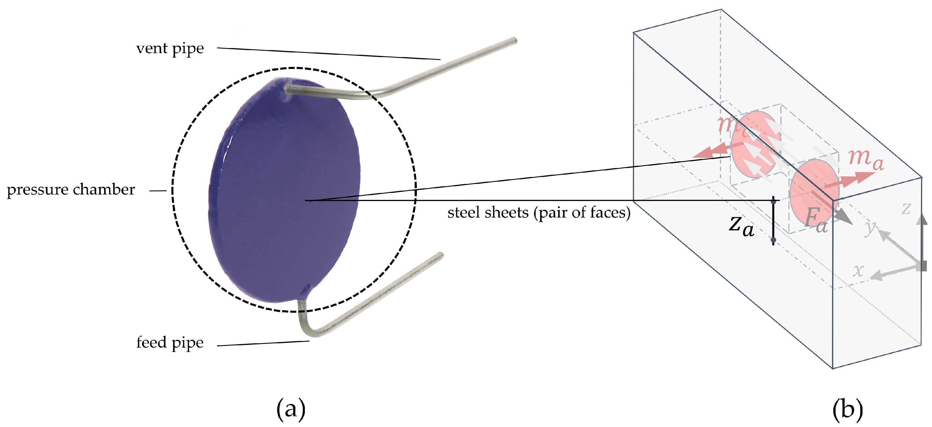
- The elaboration of a new actuation concept based on fluidic actuators that can be integrated into floor slabs to control the response under loading.
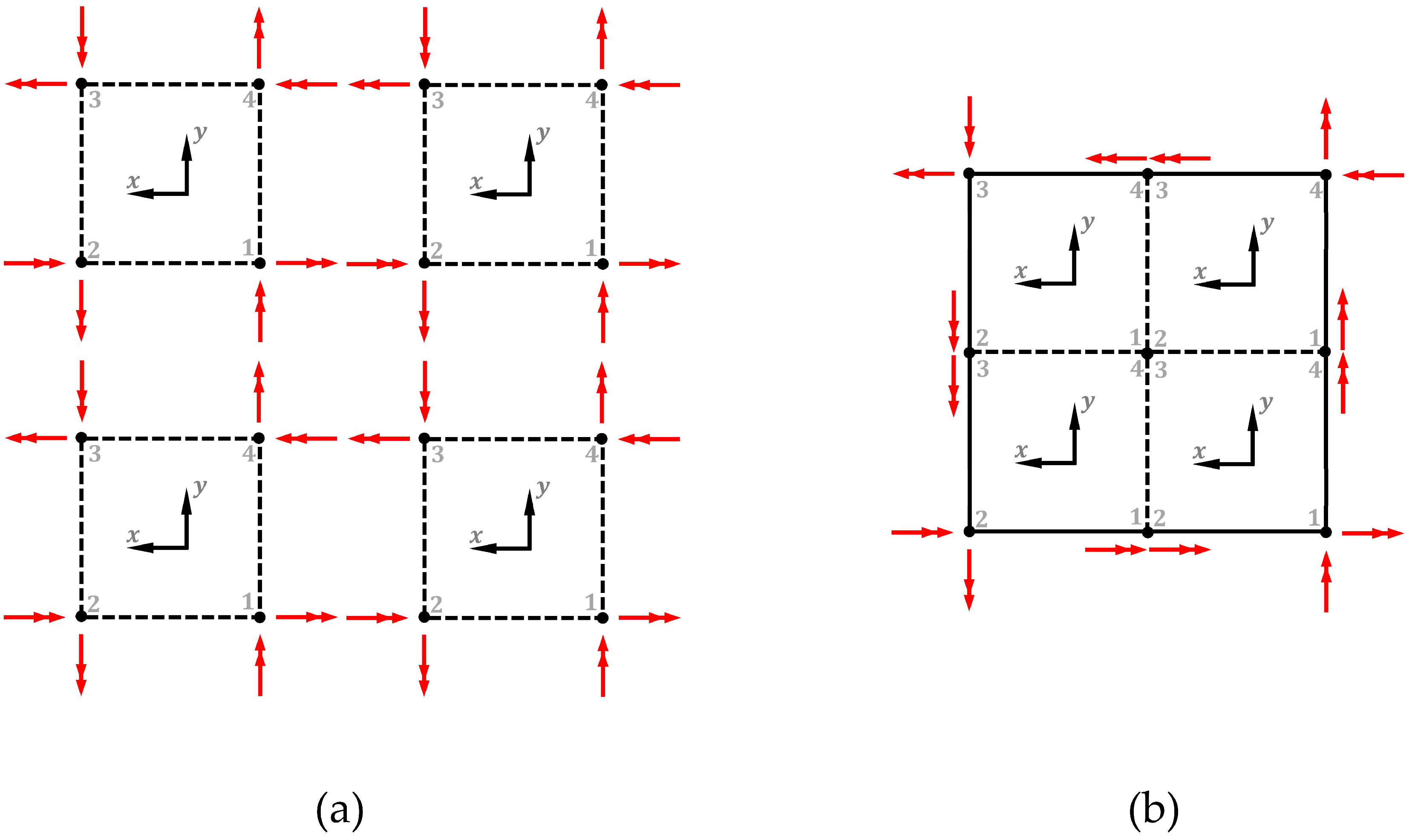
- Extension of actuation influence matrices to two-way slabs.
- Computation of actuation forces and design spaces for actuator placement based on influence matrices.
- A new methodology that makes it possible to co-design actuation and actuator concepts for adaptive floor slabs.
2. Materials and Methods
2.1. Influence Matrices
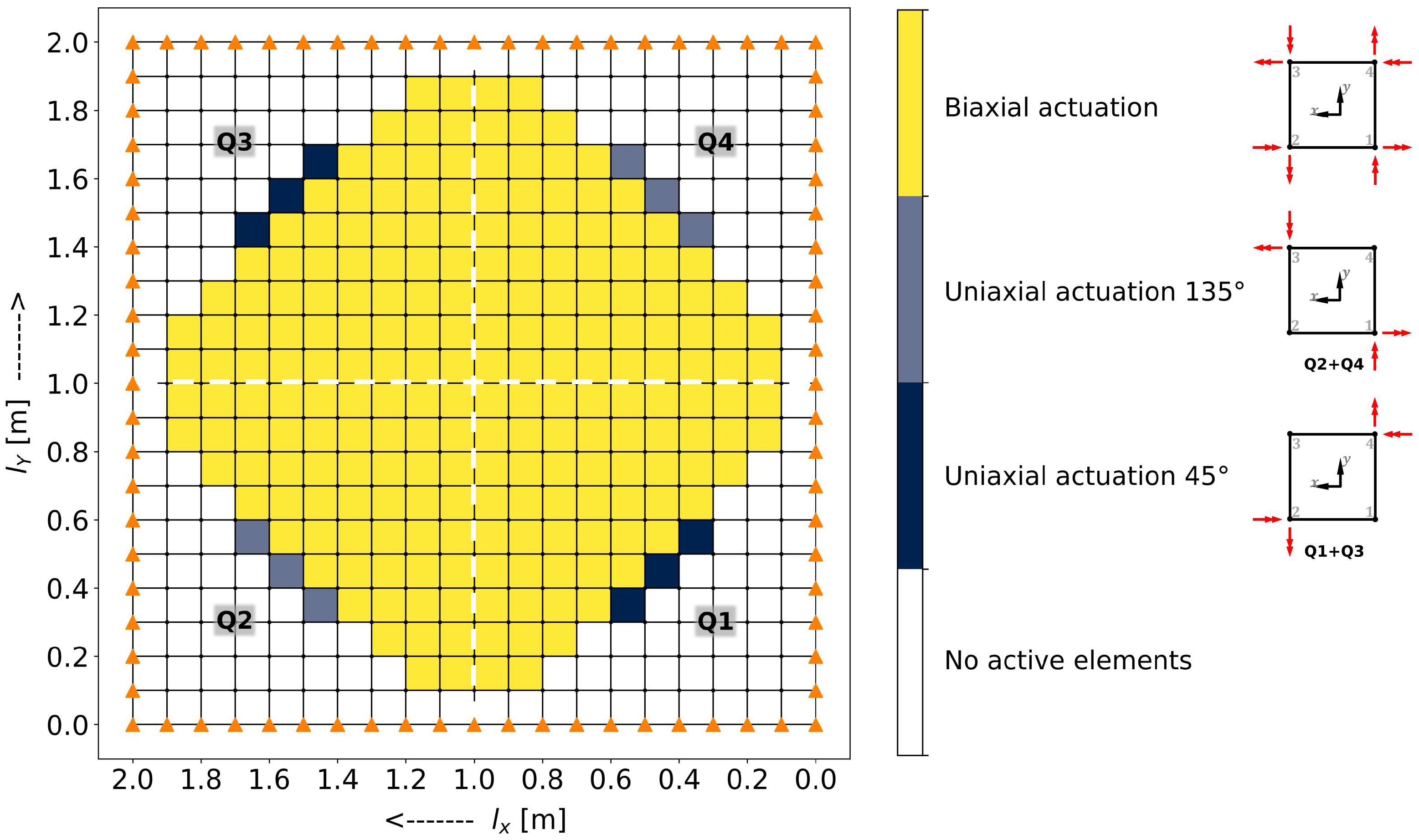
2.2. Determining Suitable Actuation Modes
2.3. Actuation Load, Adaption Level and Adaptive State
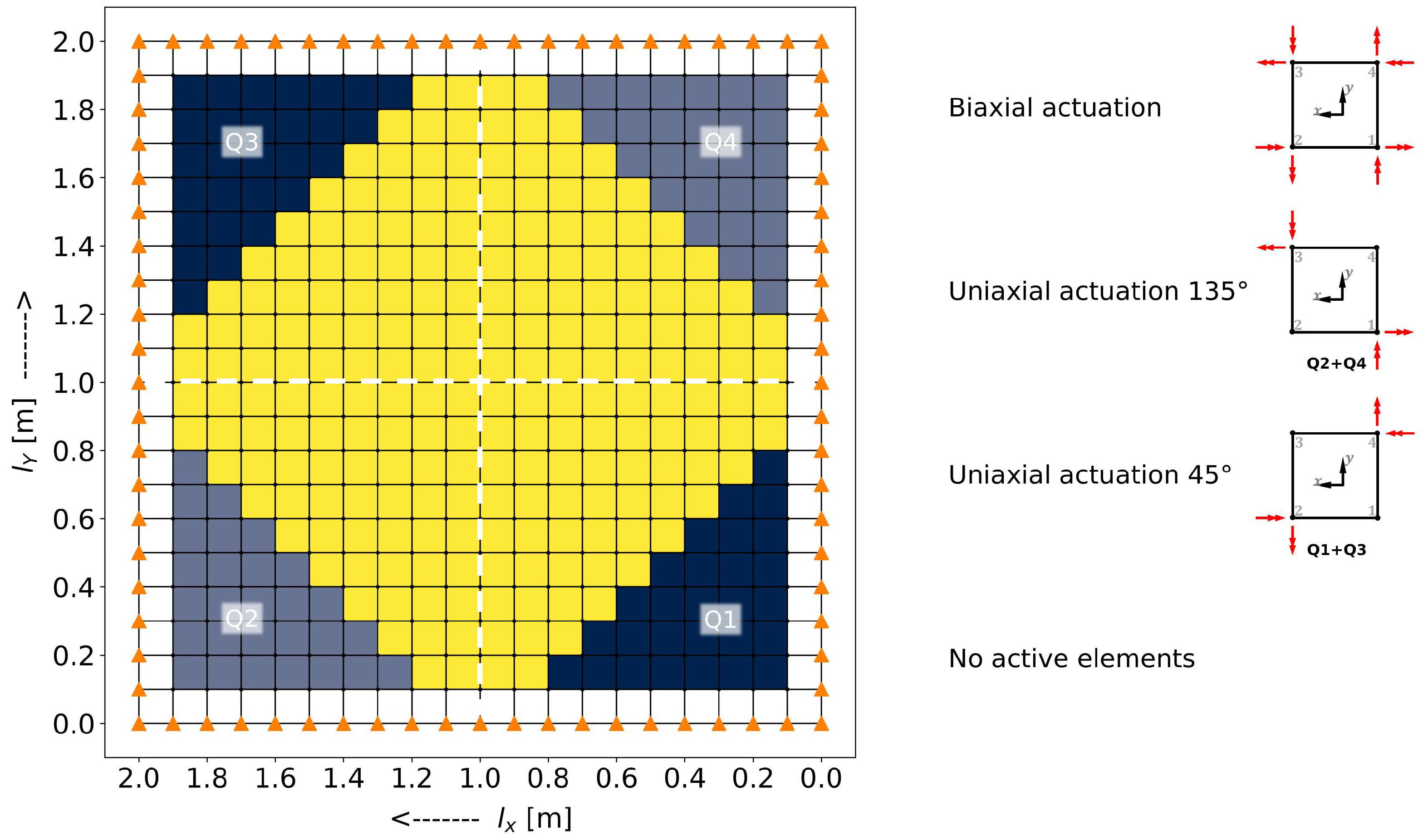
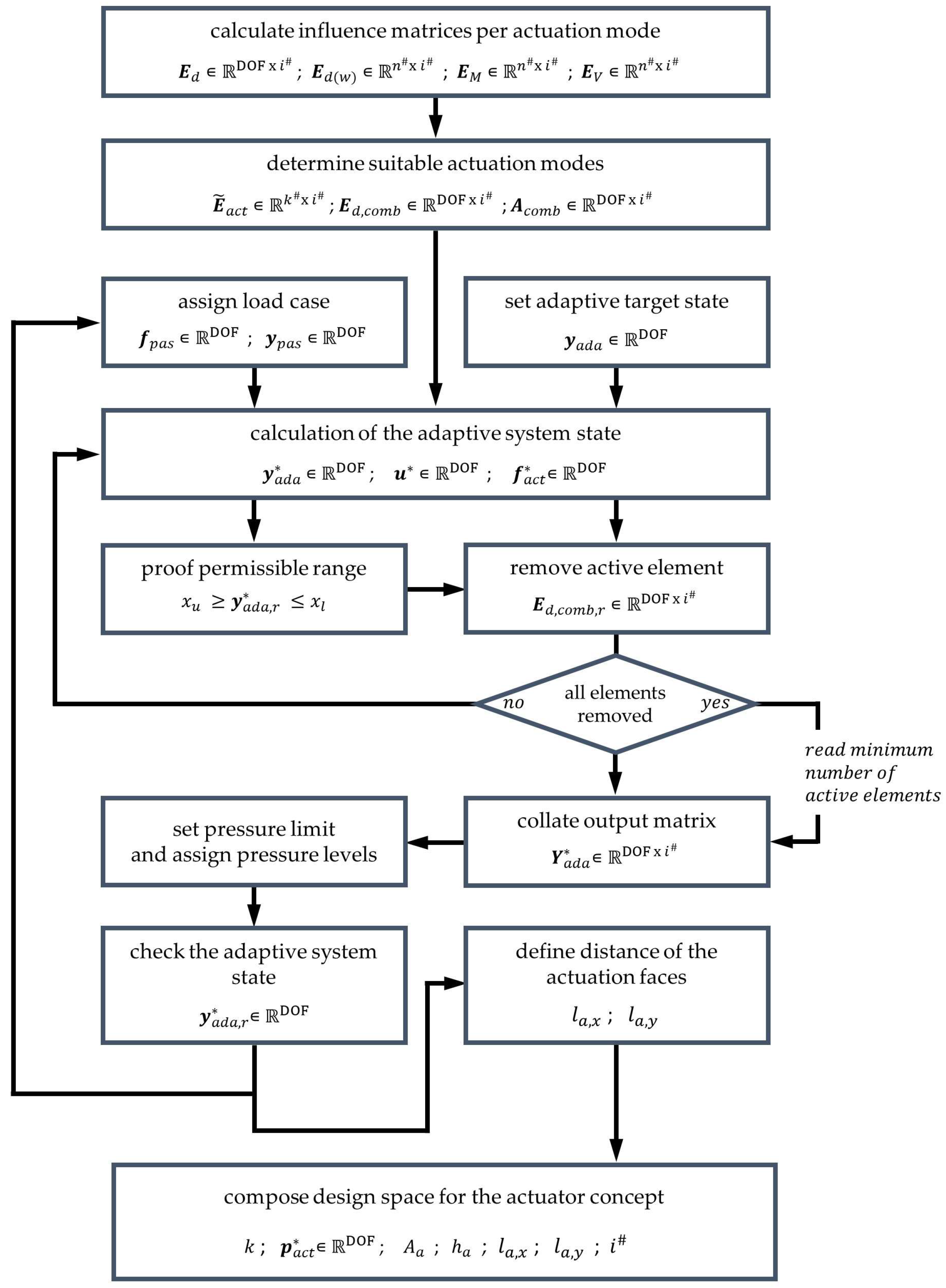
2.4. Actuator Placement
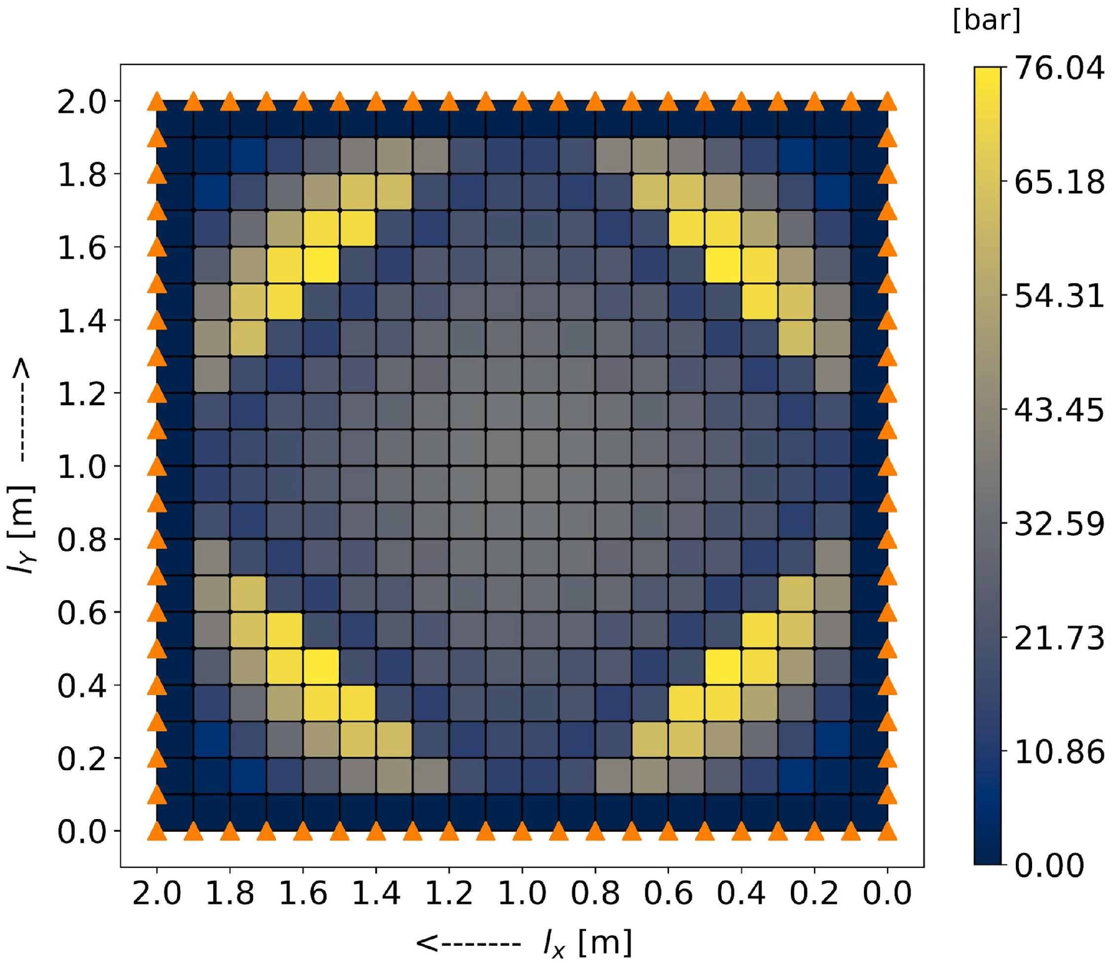
2.5. Defining Pressure Levels
3. Results
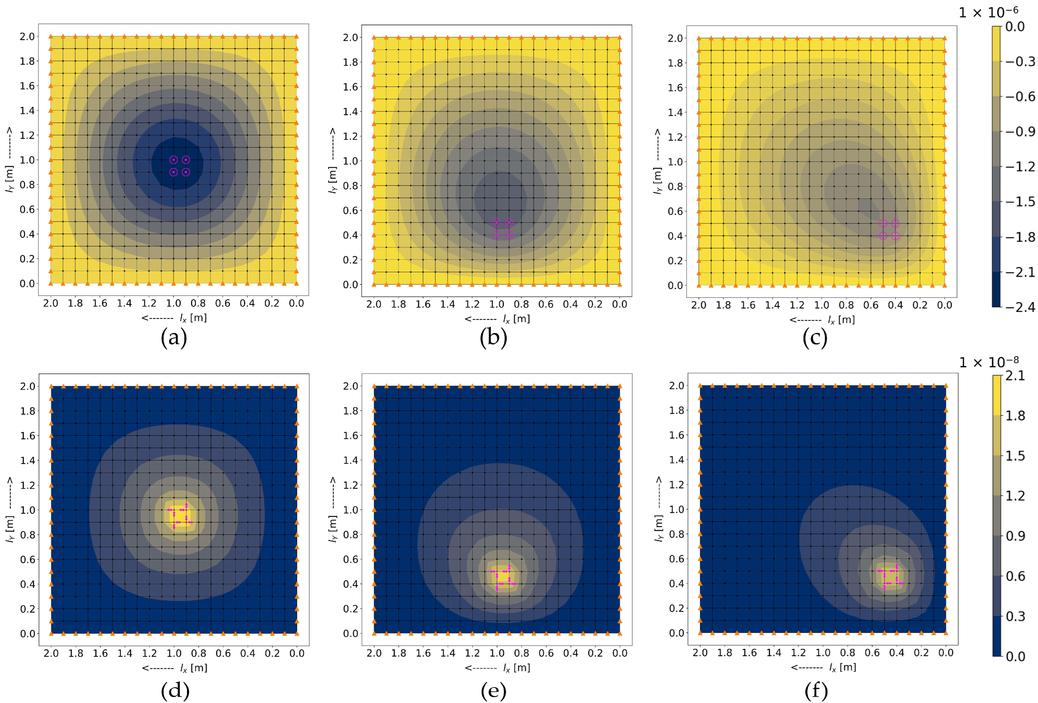
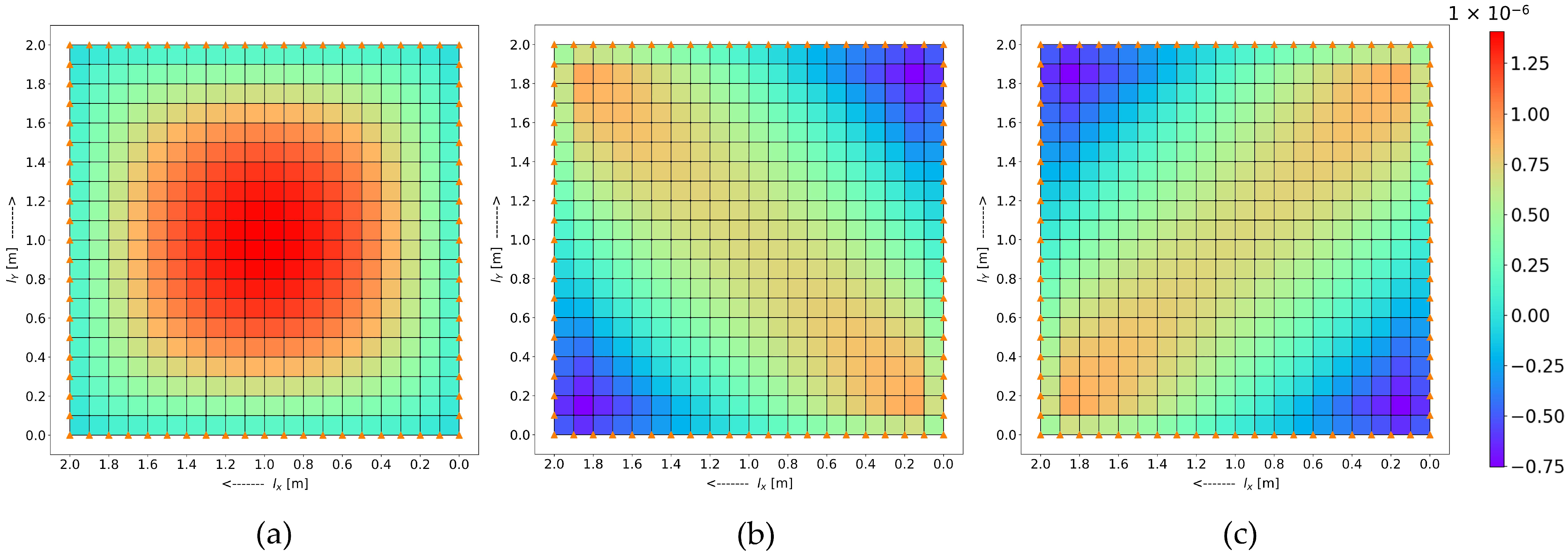
3.1. Influence Matrices
3.2. Combining Actuation Modes
3.3. Actuation Load and Adaptation Level
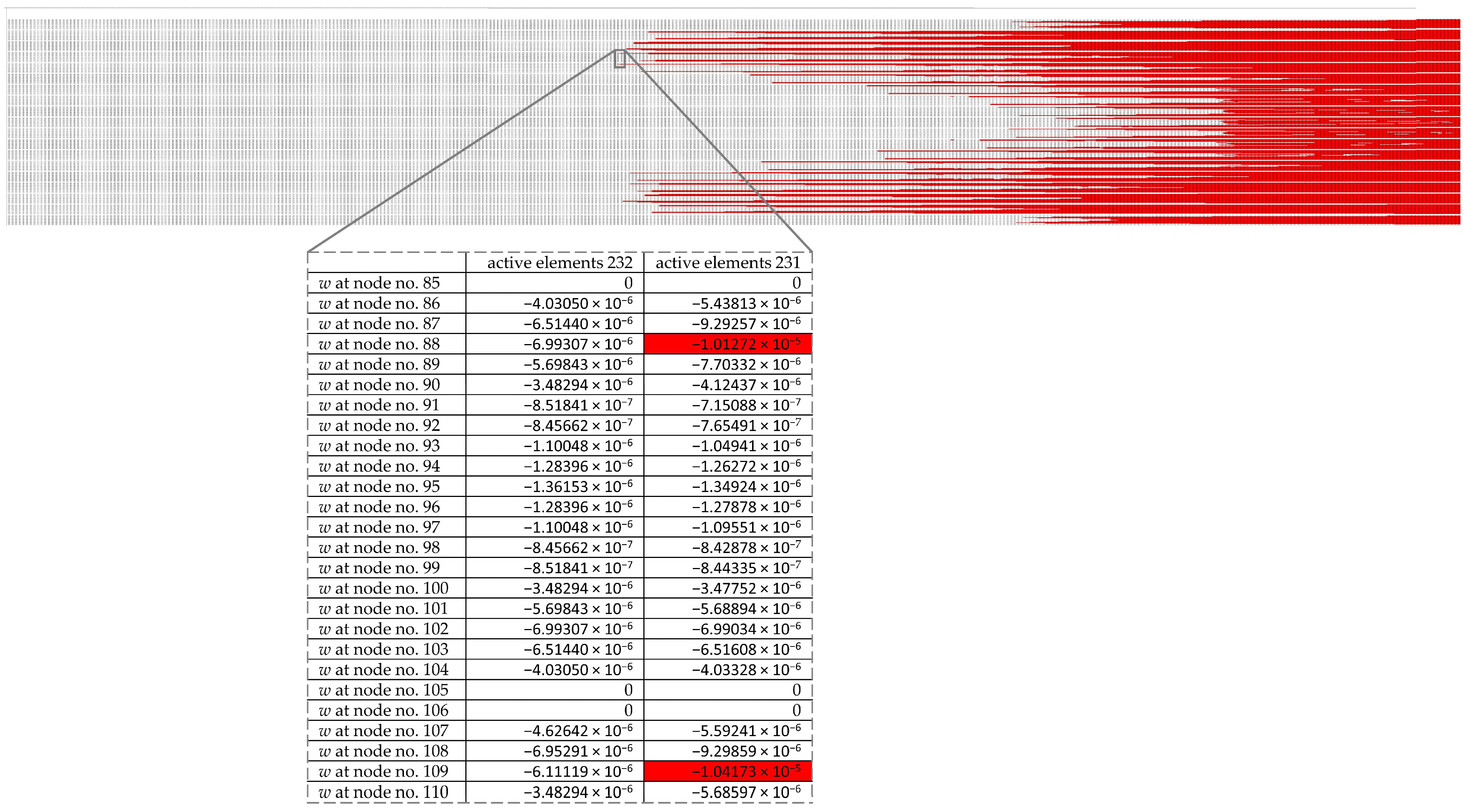
3.4. Number of Necessary Active Elements
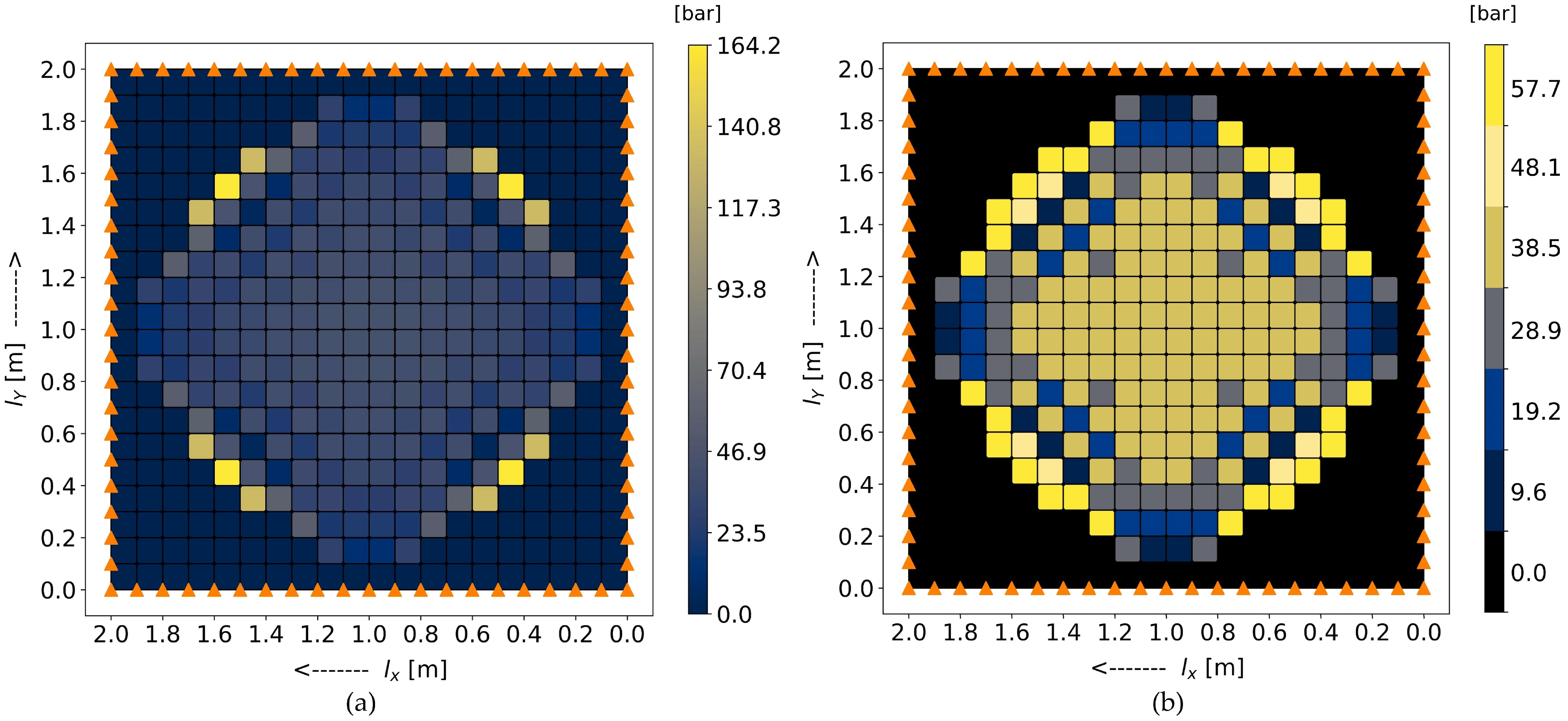
3.5. Defining Pressure Levels
4. Discussion
5. Conclusions
Author Contributions
Funding
Data Availability Statement
Conflicts of Interest
Glossary
| Sub- and Superscripts: | |
| # | indicates the total number of the respective counting variable |
| * | indicates that the vector or matrix refers to the required target state |
| DOF | degrees of freedom |
| single element, evaluation at the element corner nodes | |
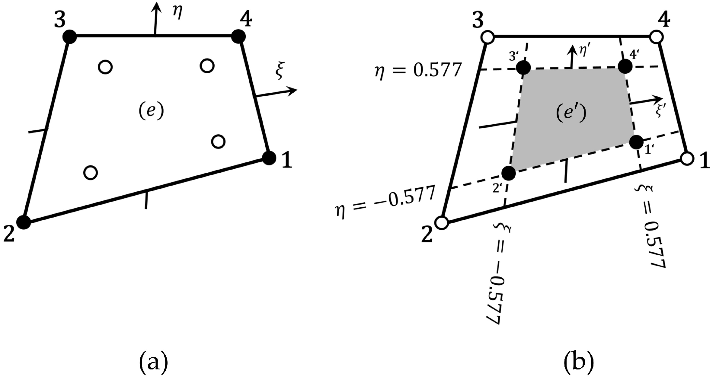
| single “gauss” element, evaluation at the gauss nodes | |
| counting variable for the active elements | |
| k | counting variable for the actuation modes |
| kmax | index of the actuation mode that has maximum influence at the respective active element |
| counting variable for the element corner nodes | |
| r | counting variable for the number of removed elements |
| Vectors: | |
| ∊ | column vector of the actuator allocation matrix. Including the actuation mode, e.g., corresponds to the uniaxial actuation mode, e.g., for element 1 |
| . ∊ ℝ 12 | element deformation vector |
| d ∊ ℝDOF | global deformation vector |
| ∊ | row vector of the summed rows of the corresponding influence column vectors of each element and actuation mode on the control objective |
| ∊ ℝDOF | column vector of the actuation influence matrix for displacements |
| ∊ | column vector of the actuation influence matrix for translational displacements w |
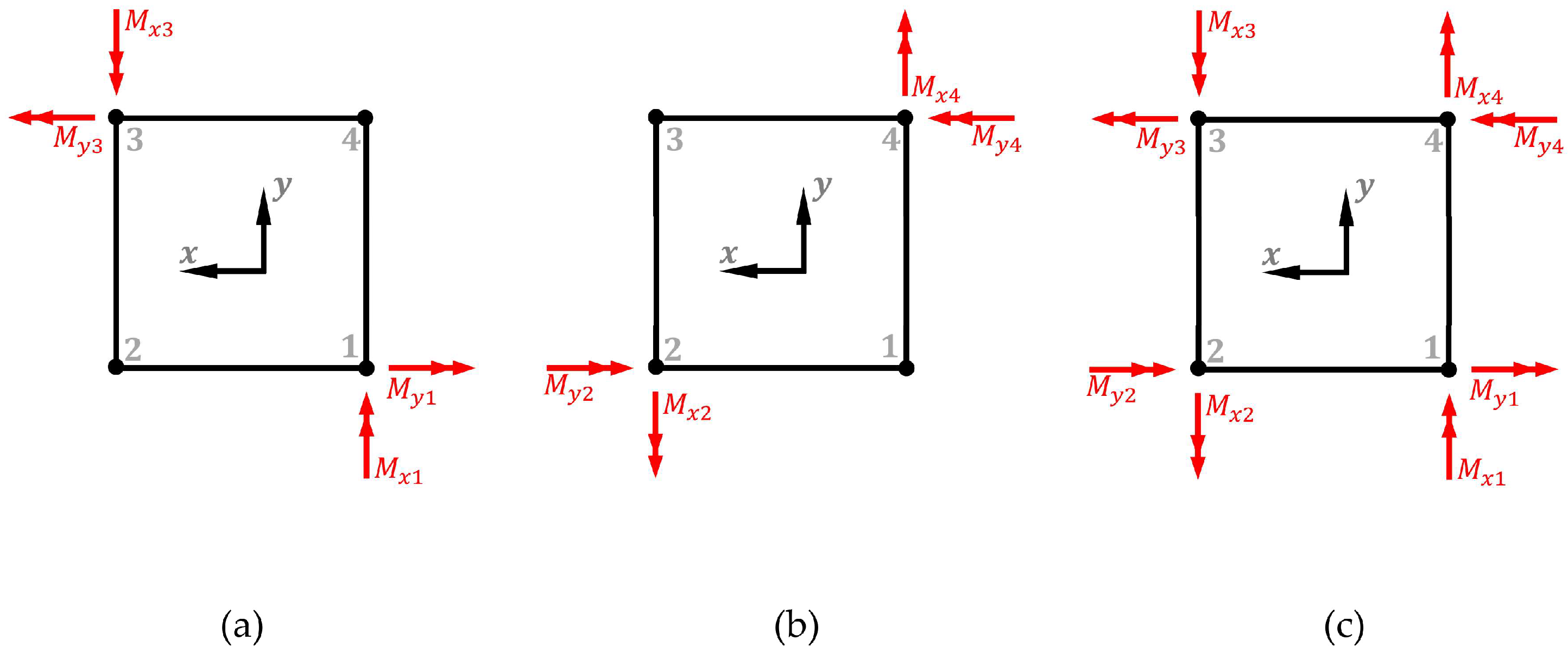
| ∊ | column vector of actuation influence matrices for the two principal moment directions |
| f ∊ ℝDOF | global force vector |
| ∊ ℝ12 | element force vector |
| ∊ ℝDOF | force vector of the required actuation moments |
| ∊ ℝDOF | global force vector for the active state |
| ∊ ℝDOF | global force vector for the passive state |
| ∊ ℝ4 | gauss node stress resultant vector for the bending moments |
| ∊ ℝDOF | actuation pressure vector |
| ∊ ℝDOF | required actuation input vector, for a target state |
| u ∊ ℝDOF | actuation input vector |
| ∊ ℝ4 | gauss node stress resultant vector for the shear forces |
| ∊ ℝDOF | output vector for the active nominal state |
| ∊ ℝDOF | output vector for the adaptive system state achievable with the actuation input |
| ∊ ℝDOF | output vector for the adaptive system state achievable with the actuation input and the current number of active elements |
| ∊ ℝDOF | output vector for the adaptive nominal state |
| ∊ ℝDOF | output vector for the passive nominal state |
| Matrices: | |
| A ∊ | actuator allocation matrix |
| ∊ | actuator allocation matrix of the combined actuation modes |
| ∊ ℝ3 x 12 | strain–displacement matrices for bending |
| ∊ ℝ3 x 12 | strain–displacement matrices for shear |
| ∊ ℝ3 x 3 | stress–strain material matrices for bending |
| ∊ ℝ2 x 2 | stress–strain material matrices for shear |
| ∊ | actuation influence matrix for the summed influences of each element and actuation mode on the control objective |
| ∊ | actuation influence matrix for displacements |
| ∊ | actuation influence matrix for displacements of the combined actuation modes with the highest summed influence |
| ∊ | actuation influence matrix for displacements of the combined actuation modes with the highest summed influence and the minimum number of active elements to stay within the target state bounds |
| actuation influence matrix for translational displacements w | |
| actuation influence matrix for bending moments | |
| ∊ | actuation influence matrices for the two principal moment directions |
| actuation influence matrix for shear forces | |
| K ∊ ℝDOF x DOF | global stiffness matrix |
| ∊ | output matrix for the adaptive system state achievable with the actuation input and the current number of active elements |
| ∊ | output matrix for the translational displacements in the adaptive system state achievable with the actuation input and the current number of active elements |
| Symbols: | |
| Moore–Penrose pseudoinverse | |
| rotational degrees of freedom | |
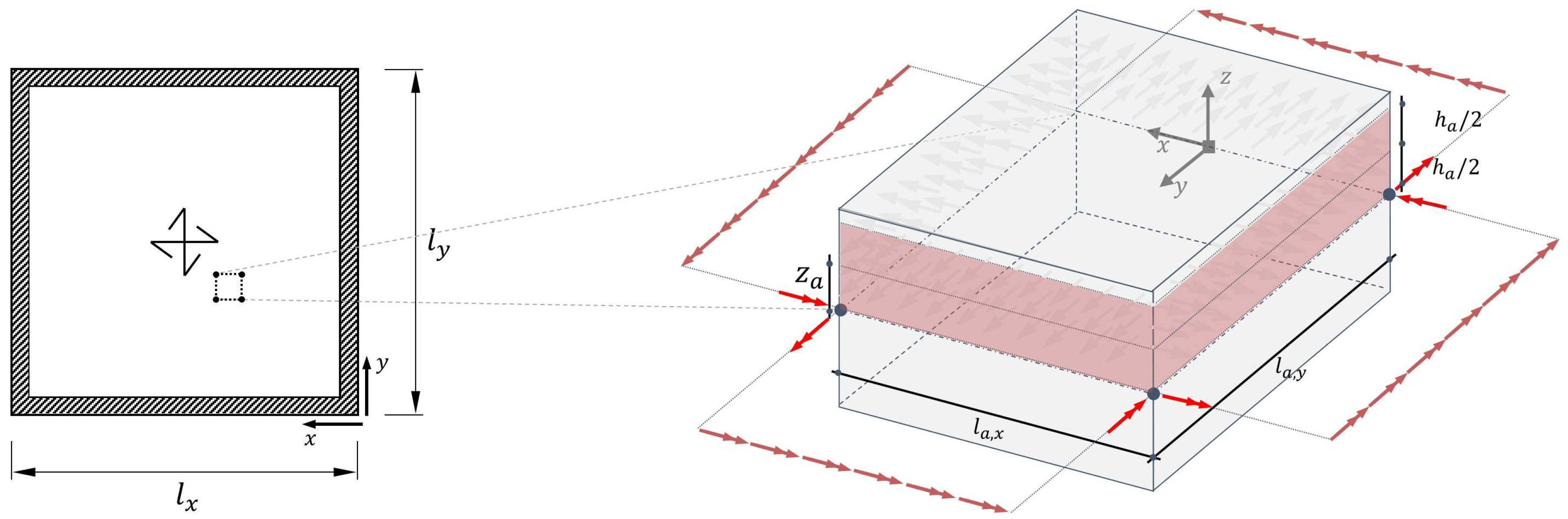
| load application area | |
| summed influence of a single element on the control objective for the respective actuation mode | |
| influence of a single element on the control objective at the respective element corner node | |
| height of the load application area | |
| edge length of a single slab element in x and y direction. Applies also when using pressure levels to form a single larger active element. | |
| span width of the slab in x and y direction | |
| w | translational displacement |
| upper limit for the translational displacement w of each node | |
| lower limit for the translational displacement w of each node | |
| inner lever |
Appendix A

References
- Sobek, W. Non Nobis—Über das Bauen in der Zukunft, Bd. 1: Ausgehen Muss Man von Dem, Was Ist; av edition: Stuttgart, Germany, 2022; ISBN 978-3-89986-369-7. [Google Scholar]
- UNEP. 2020 Global Status Report for Buildings and Construction: Towards a Zero-Emission, Efficient and Resilient Buildings and Construction Sector; UNEP: Nairobi, Kenya, 2020. [Google Scholar]
- BKI. BKI Kostenplaner 2021—Statistik Plus, Positionen; Baukosteninformationszentrum Deutscher Architektenkammern GmbH: Stuttgart, Germany, 2021. [Google Scholar]
- Berger, T.; Prasser, P.; Reinke, H.G. Einsparung von Grauer Energie bei Hochhäusern. Beton- und Stahlbetonbau 2013, 108, 395–403. [Google Scholar] [CrossRef]
- Stepan, K. Vergleichende Untersuchungen von Deckensystemen des Stahlbeton-Skelettbaus. Ph.D. Dissertation, Technische Universität München, München, Germany, 2004. [Google Scholar]
- Scrivener, K.L.; Kirkpatrick, R.J. Innovation in use and research on cementitious material. Cem. Concr. Res. 2008, 38, 128–136. [Google Scholar] [CrossRef]
- Peduzzi, P. Sand, Rarer Than One Thinks: UNEP Global Environmental Alert Service; UNEP: Nairobi, Kenya, 2014. [Google Scholar]
- WWF Deutschland. Klimaschutz in der Beton- und Zementindustrie: Hintergrund und Handlungsoptionen; WWF Deutschland: Berlin, Germany, 2019; pp. 7–11. [Google Scholar]
- Zilch, K.; Rogge, A. Bemessung von Stahlbeton- und Spannbetonbauteilen im Brücken- und Hochbau. Beton-Kalender 2004, 93, 281–283. [Google Scholar]
- Schmeer, D.; Sobek, W. Gradientenbeton. In Beton-Kalender 2019: Parkbauten Geotechnik und Eurocode 7, 108. Jahrgang; Bergmeister, K., Fingerloos, F., Wörner, J.-D., Eds.; Ernst et Sohn: Berlin, Germany, 2019; pp. 455–476. ISBN 9783433032428. [Google Scholar]
- Sobek, W. Ultra-lightweight construction. Int. J. Space Struct. 2016, 31, 74–80. [Google Scholar] [CrossRef]
- Ostertag, A.; Dazer, M.; Bertsche, B.; Schlegl, F.; Sawodny, O. Reliable Design of Adaptive Load-Bearing Structures with Focus on Sustainability. In Proceedings of the 30th European Safety and Reliability Conference (ESREL), Venice, Italy, 2–5 November 2020; pp. 4703–4710. [Google Scholar]
- Ostertag, A. Zuverlässigkeit, Sicherheit und Nachhaltigkeit Adaptiver Tragwerke; Institut für Maschinenelemente: Stuttgart, Germany, 2021. [Google Scholar]
- Yao, J.T.P. Concept of structural control. J. Struct. Div. (ASCE) 1972, 98, 1567–1574. [Google Scholar] [CrossRef]
- Domke, H.; Backé, W.; Meyr, H.; Hirsch, G.; Goffin, H. Aktive Verformungskontrolle von Bauwerken. Bauingenieur 1981, 56, 405–412. [Google Scholar]
- Soong, T.T.; Manolis, G.D. Active structures. J. Struct. Eng. 1987, 113, 2290–2302. [Google Scholar] [CrossRef]
- Neuhäuser, S.; Weickgenannt, M.; Witte, C.; Haase, W.; Sawodny, O.; Sobek, W. Stuttgart Smartshell—A full scale prototype of an adaptive shell structure. J. Int. Assoc. Shell Spat. Struct. 2013, 54, 259–270. [Google Scholar]
- Burghardt, T.; Kelleter, C.; Bosch, M.; Nitzlader, M.; Bachmann, M.; Binz, H.; Blandini, L.; Sobek, W. Investigations of a large-scale adaptive concrete beam with integrated fluidic actuators. Civ. Eng. Des. 2022, 4, 35–42. [Google Scholar] [CrossRef]
- Wang, Y.; Senatore, G. Design of adaptive structures through energy minimization: Extension to tensegrity. Struct. Multidiscipl. Optim. 2021, 64, 1079–1110. [Google Scholar] [CrossRef]
- Blandini, L.; Haase, W.; Weidner, S.; Böhm, M.; Burghardt, T.; Roth, D.; Sawodny, O.; Sobek, W. D1244: Design and Construction of the First Adaptive High-Rise Experimental Building. Front. Built Environ. 2022, 8, 4911. [Google Scholar] [CrossRef]
- Wagner, J.L.; Gade, J.; Heidingsfeld, M.; Geiger, F.; von Scheven, M.; Böhm, M.; Bischoff, M.; Sawodny, O. On steady-state disturbance compensability for actuator placement in adaptive structures. at—Automatisierungstechnik 2018, 66, 591–603. [Google Scholar] [CrossRef]
- Kelleter, C.; Burghardt, T.; Binz, H.; Blandini, L.; Sobek, W. Adaptive concrete beams equipped with integrated fluidic actuators. Front. Built Environ. 2020, 6, 107–119. [Google Scholar] [CrossRef]
- Geiger, F.; Gade, J.; von Scheven, M.; Bischoff, M. A case study on design and optimization of adaptive civil structures. Front. Built Environ. 2020, 6, 94. [Google Scholar] [CrossRef]
- Senatore, G.; Reksowardojo, A.P. Force and shape control strategies for minimum energy adaptive structures. Front. Built Environ. 2020, 6, 105. [Google Scholar] [CrossRef]
- Steffen, S.; Zeller, A.; Böhm, M.; Sawodny, O.; Blandini, L.; Sobek, W. Actuation concepts for adaptive high-rise structures subjected to static wind loading. Eng. Struct. 2022, 267, 114670. [Google Scholar] [CrossRef]
- Teuffel, P. Entwerfen Adaptiver Strukturen. Ph.D. Dissertation, Universität Stuttgart, Stuttgart, Germany, 2004. [Google Scholar]
- Schnellenbach-Held, M.; Fakhouri, A.; Steiner, D.; Kühn, O. Adaptive Spannbetonstruktur mit Lernfähigem Fuzzy-Regelungssystem: Bericht zum Forschungsprojekt 88.0107/2010; Fachverlag NW: Bremen, Germany, 2014; ISBN 978-3-95606-084-7. [Google Scholar]
- Bleicher, A. Aktive Schwingungskontrolle einer Spannbandbrücke mit pneumatischen Aktuatoren. Bautechnik 2012, 89, 89–101. [Google Scholar] [CrossRef]
- Weilandt, A. Adaptivität bei Flächentragwerken. Ph.D. Dissertation, Universität Stuttgart, Stuttgart, Germany, 2008. [Google Scholar]
- Heidenreich, C. Adaptivität von Freigeformten Flächentragwerken. Ph.D. Dissertation, Bauhaus-Universität Weimar, Weimar, Germany, 2016. [Google Scholar]
- Kleine, T.; Wagner, J.L.; Böhm, M.; Sawodny, O. Optimal actuator placement and static load compensation for a class of distributed parameter systems. at—Automatisierungstechnik 2021, 69, 739–749. [Google Scholar] [CrossRef]
- Marti, P. Baustatik: Grundlagen, Stabtragwerke, Flächentragwerke, 2. Aufl.; Ernst & Sohn: Berlin, Germany, 2014; ISBN 978-3-433-60436-3. [Google Scholar]
- Pucher, A. Einflußfelder Elastischer Platten = Influence Surfaces of Elastic Plates, 3. Aufl.; Springer: Wien, Austria; Springer: New York, NY, USA, 1964. [Google Scholar]
- Steffen, S.; Weidner, S.; Blandini, L.; Sobek, W. Using influence matrices as a design and analysis tool for adaptive truss and beam structures. Front. Built Environ. 2020, 6, 22–33. [Google Scholar] [CrossRef]
- Steffen, S.; Blandini, L.; Sobek, W. Analysis of the inherent adaptivity of basic truss and beam modules by means of an extended method of influence matrices. Eng. Struct. 2022, 266, 114588. [Google Scholar] [CrossRef]
- Kelleter, C.; Burghardt, T.; Binz, H.; Sobek, W. Actuation concepts for structural concrete elements under bending stress. In Proceedings of the 6th European Conference on Computational Mechanics (ECCM 6) and 7th European Conference on Computational Fluid Dynamics (ECFD 7), Glasgow, UK, 11–15 June 2018; Owen, R., Ed.; CIMNE: Barcelona, Spain, 2018. ISBN 978-84-947311-6-7. [Google Scholar]
- Kelleter, C.; Sobek, W.; Burghardt, T.; Binz, H. Actuation of structural concrete elements under bending stress with integrated fluidic actuators. In Proceedings of the 7th International Conference on Structural Engineering, Mechanics and Computation (SEMC 7), Cape Town, South Africa, 2–4 September 2019; Zingoni, A., Ed.; CRC Press: Boca Raton, FL, USA, 2019. ISBN 978-1-138-38696-9. [Google Scholar]
- Czichos, H. Mechatronik: Grundlagen und Anwendungen technischer Systeme, 4., überarbeitete und erweiterte Auflage; Springer: Wiesbaden, Germany, 2019; ISBN 9783658262945. [Google Scholar]
- Isermann, R. Mechatronische Systeme: Grundlagen; Springer: Berlin/Heidelberg, Germany, 2008; ISBN 978-3-540-32336-5. [Google Scholar]
- Werkle, H. Finite Elements in Structural Analysis: Theoretical Concepts and Modeling Procedures in Statics and Dynamics of Structures, 1st ed.; Springer International Publishing: Cham, Switzerland, 2021; ISBN 978-3-030-49840-5. [Google Scholar]
- Geiser, A.; Oberbichler, T.; Sautter, K. Theory of Plates—Version 1.0.1 Nov. 2017. TUM Statik: München, Germany, 2017. [Google Scholar]
- Felippa, C.A. Introduction to Finite Element Methods. In Lecture Notes for the Course Introduction to Finite Element Methods; Aerospace Engineering Sciences Department of the University of Colorado: Boulder, CO, USA, 2004. [Google Scholar]
- Housner, G.W.; Bergman, L.A.; Caughey, T.K.; Chassiakos, A.G.; Claus, R.O.; Masri, S.F.; Skelton, R.E.; Soong, T.T.; Spencer, B.F.; Yao, J.T.P. Structural control: Past, present, and future. J. Eng. Mech. 1997, 123, 897–971. [Google Scholar] [CrossRef]
- Hake, E.; Meskouris, K. Statik der Flächentragwerke: Einführung mit Vielen Durchgerechneten Beispielen, 2. Aufl.; Springer: Berlin/Heidelberg, Germany, 2007; ISBN 978-3-540-72624-1. [Google Scholar]
- Penrose, R. A generalized inverse for matrices. Math. Proc. Camb. Philos. Soc. 1955, 51, 406–413. [Google Scholar] [CrossRef] [Green Version]
- Czerny, F. Tafeln für Rechteckplatten. In Beton-Kalender 1996, Teil I; Eibl, J.W., Ed.; Ernst & Sohn Verlag: Berlin, Germany, 1996; pp. 277–330. [Google Scholar]


| Properties | Value | Unit |
|---|---|---|
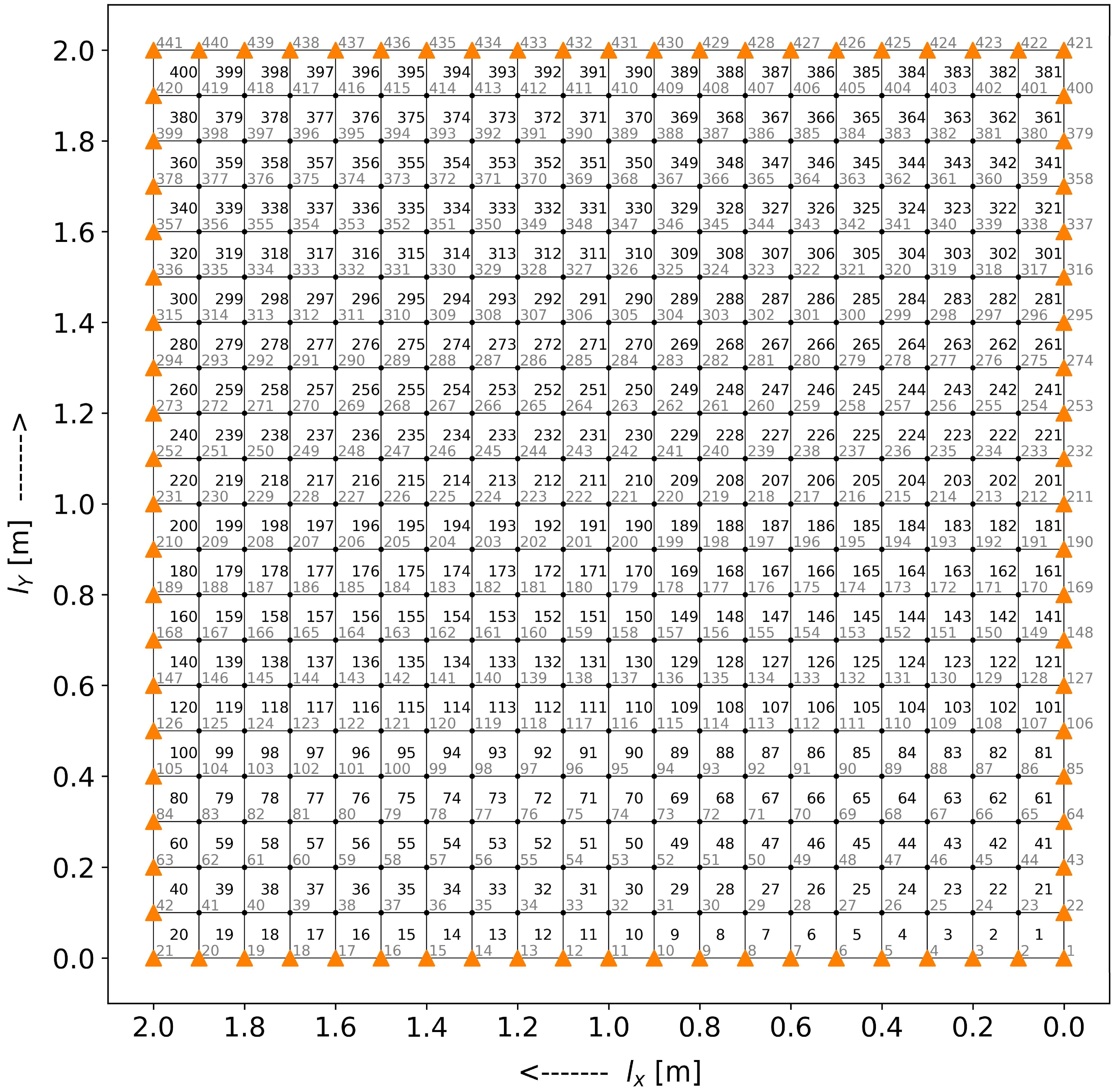
| Span | 2 | m |
| Thickness | 0.1 | m |
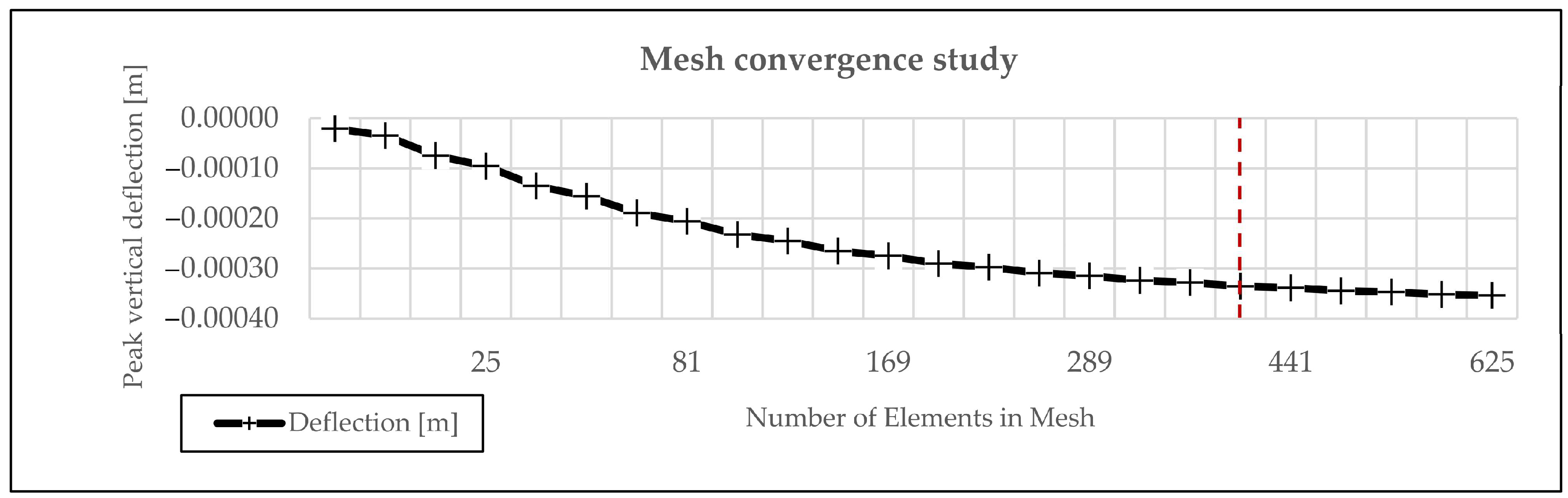
| Elementsize | 0.1 | m |
| E-modulus | 30 | GPa |
| Poisson’s ratio | 0.2 | - |
Publisher’s Note: MDPI stays neutral with regard to jurisdictional claims in published maps and institutional affiliations. |
© 2022 by the authors. Licensee MDPI, Basel, Switzerland. This article is an open access article distributed under the terms and conditions of the Creative Commons Attribution (CC BY) license (https://creativecommons.org/licenses/by/4.0/).
Share and Cite
Nitzlader, M.; Steffen, S.; Bosch, M.J.; Binz, H.; Kreimeyer, M.; Blandini, L. Designing Actuation Concepts for Adaptive Slabs with Integrated Fluidic Actuators Using Influence Matrices. CivilEng 2022, 3, 809-830. https://0-doi-org.brum.beds.ac.uk/10.3390/civileng3030047
Nitzlader M, Steffen S, Bosch MJ, Binz H, Kreimeyer M, Blandini L. Designing Actuation Concepts for Adaptive Slabs with Integrated Fluidic Actuators Using Influence Matrices. CivilEng. 2022; 3(3):809-830. https://0-doi-org.brum.beds.ac.uk/10.3390/civileng3030047
Chicago/Turabian StyleNitzlader, Markus, Simon Steffen, Matthias J. Bosch, Hansgeorg Binz, Matthias Kreimeyer, and Lucio Blandini. 2022. "Designing Actuation Concepts for Adaptive Slabs with Integrated Fluidic Actuators Using Influence Matrices" CivilEng 3, no. 3: 809-830. https://0-doi-org.brum.beds.ac.uk/10.3390/civileng3030047