
Optimal Relabeling of Water Molecules and Single-Molecule Entropy Estimation


1
Dipartimento di Scienze Matematiche, Informatiche e Fisiche (DMIF), University of Udine, Via delle Scienze 206, 33100 Udine, Italy
2
Science and Math Division, New York University at Abu Dhabi, Abu Dhabi P.O. Box 129188, United Arab Emirates
*
Author to whom correspondence should be addressed.
†
Current address: Istituto Nazionale Biostrutture e Biosistemi, Viale Medaglie d’Oro, 305, 00136 Roma, Italy.
Biophysica 2021, 1(3), 279-296; https://0-doi-org.brum.beds.ac.uk/10.3390/biophysica1030021
Submission received: 15 May 2021
/
Revised: 21 June 2021
/
Accepted: 23 June 2021
/
Published: 30 June 2021
(This article belongs to the Special Issue Role of Water in Biological Systems)
Abstract
:Estimation of solvent entropy from equilibrium molecular dynamics simulations is a long-standing problem in statistical mechanics. In recent years, methods that estimate entropy using k-th nearest neighbours (kNN) have been applied to internal degrees of freedom in biomolecular simulations, and for the rigorous computation of positional-orientational entropy of one and two molecules. The mutual information expansion (MIE) and the maximum information spanning tree (MIST) methods were proposed and used to deal with a large number of non-independent degrees of freedom, providing estimates or bounds on the global entropy, thus complementing the kNN method. The application of the combination of such methods to solvent molecules appears problematic because of the indistinguishability of molecules and of their symmetric parts. All indistiguishable molecules span the same global conformational volume, making application of MIE and MIST methods difficult. Here, we address the problem of indistinguishability by relabeling water molecules in such a way that each water molecule spans only a local region throughout the simulation. Then, we work out approximations and show how to compute the single-molecule entropy for the system of relabeled molecules. The results suggest that relabeling water molecules is promising for computation of solvation entropy.
1. Introduction
The estimation of free energy and entropy from molecular dynamics calculations is a long-standing problem in biomolecular simulations [1,2,3,4,5,6,7,8].
Pathway methods [9] based on free-energy perturbation [10] or thermodynamic integration [11] are accurate but difficult to apply for large systems, moreover linking the results of the calculation to single molecular components is difficult.
Entropy can be also computed from the dependence of the computed solvation free energy, or using pathway methods using the proper integrand [12].
In this work, we focus on ensemble methods, which display large fluctuations, and therefore converge slowly, but may be applied also to large systems and allow in principle to link the results to all the degrees of freedom of the system.
Treatment of solvation with ensemble methods is challenging due to the large number of correlated degrees of freedom. Most solvation theories have been proposed based on distribution functions, which are accessible experimentally and can be easily visualized. In this context, inhomogeneous fluid solvation theory (IFST) [13,14], has provided the theoretical reference frame for a number of applications such as WaterMap [15,16], GIST [17,18], SSTMap [19]. Other used models, which depart from straightforward solvent simulation analysis, include Grand Canonical Monte Carlo simulations [20], the reference interaction site model (3D-RISM) [21] and other methods as recently reviewed [22].
Molecular dynamics simulations provide a large number of configurational samples from which single-molecule distribution functions can be computed. Such distribution functions are more practical; however, less informative than the actual set of configurations recorded in a simulation.
Because in molecular dynamics simulations, the enthalpy is obtained as the ensemble average of the recorded energy, the problem of estimating the free energy of a system is essentially that of estimating the entropy, demonstrating the importance of this task.
In the last decade, methods based on the k-th nearest neighbour [23] (kNN) to compute the entropy of a system based on the k-th nearest neighbour have been proposed and applied to solutes and solvent. Most applications of the kNN methods have concerned internal degrees of freedom [17,24,25,26,27,28,29,30,31,32] although the method was also used for computing positional-orientational entropies [17,30,32,33,34,35,36,37,38,39,40,41,42]. The latter applications required in turn to define a distance in positional-orientational (most commonly refered to as translational-rotational) space [35,37], and the study of an accurate approximation of the volume of a ball in such a six-dimensional space [37,38].
The application of the kNN method, and other methods for entropy estimation, has been complemented by approximations to deal with the high-dimensionality of the configurational space of typical biomolecular systems. In particular, first Gilson and co-workers developed the mutual information expansion (MIE) [26,43] and later, the Maximum Information Spanning Tree approach by Tidor and co-workers [44] was applied by the same authors [45,46] and others [30,47,48,49,50] to entropy estimation.
Here, we focus on specific issues connected to the application of the approach to solvent molecules. For the sake of illustration, we will consider water but the treatment will be generally applicable to other solvent molecules.
For what concerns water, Berne and coworkers [27] used before the k-th nearest neighbour method to compute the Shannon pairwise orientational entropy. The correlation among positional and orientational degrees of freedom was simplified considering three distance ranges, and the orientational degrees of freedom were reduced from five to four by neglecting the dihedral angle defined by the rotation of one water molecule dipole about the oxygen–oxygen interatomic vector with respect to the other water molecule. The framework and the approximations followed previous work by Lazaridis and Karplus [51].
The remaning four angular dimensions were treated by repeated application of the generalized Kirkwood superposition approximation [52], resulting in formulae containing joint probabilities of at most two variables. After suitable changes of variables, they could estimate two-dimensional entropies by using the kNN approach, providing an accurate estimate of the excess entropy of water.
In the application of the kNN method to water molecules, a significant improvement was the consideration of distances in the six-dimensional translation-rotation space [35,37], which removed the need to decouple positional and orientational coordinates. In our previous work, the correctness of the approach and its accuracy were demonstrated [37] and recently extended to two translation-rotations [38].
Along this line, Irwin and Huggins [40] presented the application of the kNN method to the solvation of a Lennard–Jones molecule in neon in the context of the inhomogeneous fluid solution theory (IFST), which is based in turn on a generalization of the Kirkwood approximation [53].
Recently the unbinned weighted histogram analysis method (UWHAM) approach by Levy and coworkers [54,55] led to very accurate (95%) estimation of excess solvation energies from end-point simulations or just with the addition of one intermediate state. The approach focuses on a single water molecule at a time at fixed position, e.g., a crystallographic solvated water.
Compared to the latter and other methods, the analysis presented here differs in one basic aspect: our aim here is to define a framework to turn a problem involving indistinguishable molecules spanning the whole configurational space into a problem involving distinguishable molecules, each spanning a localized configurational space. If this task can be accomplished, one can treat solvent entropy based on the kNN and MIST methods, on the same ground as for other biomolecular systems with a large number of correlated degrees of freedom. To do this, we focus on mapping the problem involving indistinguishable solvent molecules into a problem where solvent molecules retain their identity, which is done here via a relabeling of water molecules and hydrogen atoms.
After this paper was first submitted, we became aware that a similar approach was proposed by Reinhard and Grubmüller in the context of the quasiharmonic approximation [56] and very recently by Heinz and Grubmüller [41,42]. The approach described here differs in that it is built on the exact theory developed previously for the kNN method applied to translation-rotations [8,37] and the entropy calculation after relabeling is not based on pairwise distances between relabeled molecules, but rather on the distances from chosen references.
Here, we outline the relabeling method, apply this to pure water and water around a fixed water molecule, and highlight its features in relation to entropy estimation.
The paper is organized as follows: (i) the k-th nearest neighbour method is summarized; (ii) the metric in single-molecule translational-rotational space is reviewed; (iii) the distance between single molecules is used to define a distance between ensembles of molecules, thus providing a criterion (the search for minimal distance) to optimally relabel indistinguishable molecules (and atoms); (iv) the hungarian algorithm for optimal relabeling of solvent molecules is reviewed; (v) the original problem of the computation of entropy on the ensemble of indistinguishable molecules is mapped to the problem of the computation of entropy on the ensemble of relabeled and localized molecules (and atoms). The approximations under which the equations are valid are discussed; (vi) the systems and the simulations used to test the theory are described; (vii) results are presented and discussed.
2. Methods
2.1. The K-th Nearest Neighbour Method for Entropy Estimation
The k-th nearest neighbour method has been proposed by Kozachenko and Leonenko [57] and further developed and corrected by Demchuk and coworkers [23]. We have recently reviewed the method and its practical implementation [38], we summarize here the main features of the method. The central idea is that the local density of a distribution may be estimated by constructing a ball with radius equal to the distance from each of n samples to its k-th nearest neighbour. Since the ball contains k samples, the probability density is reasonably estimated by:
and therefore, if is the volume of the ball centered at sample i, with radius up to its k-th nearest neighbour, the probability density at each sample is reasonably estimated by the following:
The entropy, which is expressed as follows:
is thus naively estimated by the ensemble average of , i.e.,
Demchuk and coworkers [23] worked out the exact theory based on this idea and found the unbiased estimator:
where plays the role of in the naive formula and is defined iteratively by , and is the Euler–Mascheroni constant (0.5722…).
It is crucial, for the application of the method, that it is possible to compute the volume of a ball in the space of samples, which is not in general as straightforward as in euclidean spaces. The next subsection addresses this issue for the single-molecule translational-rotational space.
2.2. Metric in Translational-Rotational Space
The metric in the translational-rotational space of one and two molecules has been addressed in our previous work [37,38], we resume here the main properties.
The definition of distance in translational-rotational space combines the distance in translational space with that in rotational space. Many definitions of a metric in the space of rotations are possible with different properties [58]. The distance in rotational space can be combined with the translational space distance according to the euclidean product metric [59], which can be shown to be a metric. Such a way of combining the two distances into a single distance was first proposed by Huggins [35] and we introduced the idea of using a length to make the two distances homogeneous, and provided the formula for the volume of a ball in translational-rotational space [37] and its approximation for use in the kNN approach.
We represent the translation-rotation state of a molecule by a translation vector, , and a rotation matrix, R, with respect to a fixed frame of reference.
A natural definition of distance in rotation space is given by [33,58,60]:
where the subscripts indicate solvent molecule a and b, respectively, and indicates trace operation.
If two solvent molecules (say a and b) are superimposed to a reference one by rotation and translation , we define their compound distance d in translational-rotational space as follows [35,37]:
where, the subscripts indicate solvent molecules a and b, respectively, and l is a length for making translational and rotational distances homogeneous. The latter can be chosen arbitrarily, in principle, but it is convenient to have a similar weight for cartesian and angular components of the compound distance.
Furthermore, if there are symmetric parts in the molecule, the distance may be chosen as the minimum distance among all possible symmetrically related configurations.
2.3. Distance in the Configurational Space
The configuration of a system of indistinguishable molecules may be described by a class of equivalence, including all possible permutations of their labels. If solvent molecules display symmetry, all symmetrical configurations must be included in the same class of equivalence.
Since any permutation of labels will be consistent with the same system configuration, it is not obvious how to define a distance, at variance with the case where molecules are distinguishable. For instance, the root mean square deviation (RMSD) between molecules with the same labels would result in distances larger than zero for the same configuration with different labeling. A similar consideration applies to symmetry-related molecular configurations.
For this reason, we must first define a distance independent of both labeling and molecular symmetry operations.
In order to do this, we first choose a reference configuration (e.g., one of the configurational samples, but it could also be a regular arrangement of the system or a minimized configuration). Then, the labels of the molecules in each configuration are permuted and symmetry operations are performed in such a way that the distance (defined hereafter) from the reference configuration is minimal.
Using the distance in rotational-translational space defined for the single molecule in the previous section, we define the distance () between two different labeled configurations as the sum of the distances, of each labeled molecule i in one configuration from the molecule with the same label i in the other configuration:
and we find the permutation of indices, which among all permutations P of the sample molecules is the one that makes minimal. This is executed algorithmically as detailed in the next section.
The distance between two configurations is defined as follows:
Note that if the defined single-molecule distance is a metric, it can be shown that the minimal distance d between the two configurations defines a metric in the space of configurations.
The definition of a distance between samples is necessary to provide an optimal criterion for relabeling solvent molecules, which is described in the next subsection. Using the relabeled system, we show how single-molecule entropy can be computed, as detailed in the following sections.
2.4. Optimal Relabeling of Molecules
Relabeling molecules aims at transforming the indistiguishable molecules system into a system where all molecules are labeled and span a localized configurational region. We choose a reference configuration where each water molecule has its own label. We sort all molecules by their distance from the solute and renumber accordingly the water molecules in each configuration obtained from snapshots from molecular dynamics simulations. Then, for each configuration, we aim at relabeling each water molecule in such a way that the configuration distance from the reference configuration, i.e., the sum of each molecule distance between the two configurations (see previous subsection), is minimal.
The problem is not trivial and here it is recast in the framework of the assignment problem that deals with the optimal assignment of N (or more) tasks to N persons, with costs that vary depending on the task and on the person.
In other words, this amounts to assigning each different task i to each different person labeled j in such a way that the set of assigments , with , is a permutation of labels , i.e., each task is assigned to a single person and each person is assigned a single task.
Here, the cost of assigning molecule j of the snapshot configuration to molecule i of the reference configuration is the distance in translational-rotational space.
Another way of looking at this problem, which leads us directly to our problem, is the following: we have a cost matrix with N rows and N columns and we look for a one-to-one mapping of rows onto columns.
In our relabeling problem, we set up the cost matrix by assigning the distance from each solvent molecule (column) in the sample configuration to each solvent molecule (row) in the reference configuration. The minimal cost found by the assignment algorithm will be the sum of distances in Equation (10). The problem is solved by the so-called Hungarian algorithm [61,62].
2.5. The Hungarian Algorithm
The Hungarian algorithm finds the best matching between columns and rows of a cost matrix such that the sum of costs is minimal.
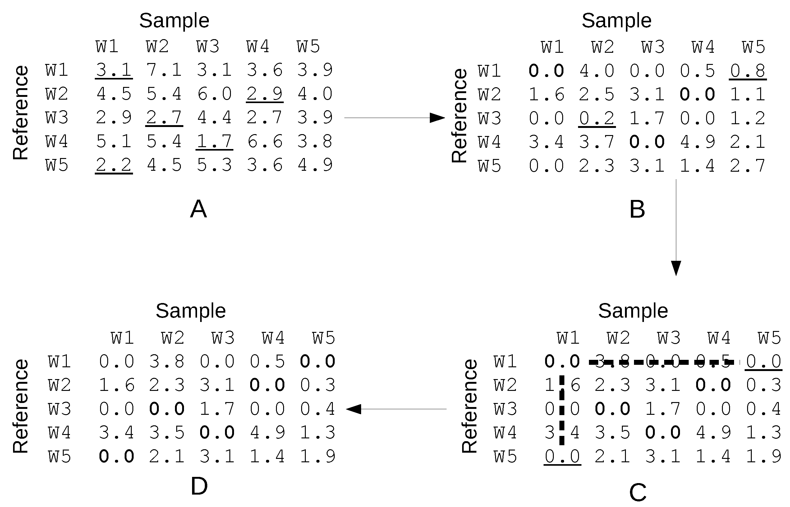
For the sake of illustration, consider the matrix in the panel A of Figure 1 where for each of the five molecules W1, W2, W3, W4 and W5 in the reference configuration, all costs (i.e., the distances from all the same five molecules in the sample configuration) are reported.
The task is to find the one-to-one correspondence of molecules in the reference to the ones of the sample configuration such that the total cost is minimal.
The Hungarian algorithm uses two key concepts: (i) if we add or subtract a constant cost to a row, the solution is not affected (i.e., if all distances of a reference molecule to all sample molecules are increased by the same amount, the costs of all assignments will be equally affected); (ii) if we add or subtract a constant cost to a column, the solution is not affected (by the same token as for the rows).
The algorithm proceeds iteratively using these ideas and finding intermediate tentative assignments whose number can be augmented at each step until a complete assignment is found. All details are reported in a book by Knuth [62] (ASSIGN_LISA algorithm), and are too elaborate to be described here. The elements of the algorithm are sketched in Figure 1.
At the end of the algorithm, each solvent molecule is relabeled in such a way as to make the distance from the reference configuration minimal.
2.6. Entropy Calculation after Relabeling
We assume that the solvent molecules are sufficiently rigid as to treat them as rigid bodies as far as intermolecular interactions are concerned.
The classical partition function of N nearly rigid interacting bodies, assuming intramolecular interactions decoupled from intermolecular interactions and neglecting possible symmetries is
where and are the momentum integral and the partition function for intramolecular interactions, and is the classical configurational integral:
where describes intermolecular interactions.
Momentum and intramolecular interactions integrals factor out and cancel out upon comparison of different macrostates of the same system at the same temperature. Since we assume nearly rigid molecules, we consider only positional and orientational coordinates indicating as all the six variables refering to water molecule i (e.g., center of mass position and axis-angle of rotation with respect to a reference system).
For such a system, the configurational entropy is given by
with
We can partition the ith single-molecule integration space in N (equal to the number of molecules) disjoint domains , where the first index refers to the molecule and the second indicates the domain, covering the integration space. The same partitioning is applied to all molecules’ configurational space. The N-molecule space can thus be written as the product of the spaces of each molecule.
The configurational integral may be rewritten accordingly as
where stands for all possible combinations of indices .
In order to proceed further, we make a key assumption, for which the limits will be assessed later: we assume that the density of the molecules is so high that each of the domains contains one, and only one, molecule.
This implies that all integrals over domains in the product in which results in a zero contribution to the integral, which implies in turn that only combinations of indices that are permutations of the indices contribute the integral. Thus, the summation is restricted to the set of permutations of the indices ().
Since all molecules are indistinguishable, indices may be permuted without affecting the integral; the latter can be rewritten as
with indices permuted in such a way that molecule 1 is in , molecule 2 is in , …, molecule N is in .
In order to establish a correspondence between the permutation and the relabeling discussed in the first sections, we now define a new probability distribution , with if and 0 if . All variables are thus locally and disjointedly distributed, in such a way that
To complete this picture, let us denote the probability distributions of each relabeled molecule, which are all localized and different, as .
The probability density that any of the molecules is found at x, , is given by the integral of the distribution over other particles and a factor N corresponding to the number of possibilities for the first index:
The latter equation will be useful to calculate the single-molecule entropy.
The entropy of the localized probability distribution is related to the entropy S of the probability distribution of N indistingushable molecules, under the assumption of disjoint configurational domains, by the equation:
Now, the original problem involving indistinguishable molecules has been turned into a problem where molecules span localized spaces and the factor linked to permutation of indistinguishable molecules cancels out. Although extremely difficult, the problem, cast in this way, can now be faced with tools such as MIE or MIST, which deal with the entropy of many-variables probability distributions.
2.7. Single-Molecule Entropy Calculation after Relabeling
After relabeling, the set of molecules with the same labeling are the first nearest-neighbours (compatible with one-to-one correspondence of labels) with respect to the reference configuration and define, along the trajectory, an ensemble of configurations distributed according to the function defined in the previous subsection.
For each snapshot, molecules are first renumbered, with lower numbering according to the lesser distance from the solute or from a set of fixed coordinates.
The ensemble of configurations is dependent on the reference configuration chosen. In order to average over possible reference configurations, 100 snapshots were taken from the simulation and for each of these snapshots, water molecules of the other 9999 snapshots (including also the other 99 snapshots chosen for averaging) were optimally relabeled using the Hungarian algorithm as described above and in the reference cited.
The pairwise distances between molecules in each ensemble of configurations (one for each molecule and for each of the reference configurations) were used to estimate the single-molecule entropies according to the k-th nearest neighbour method, applied to the 6N dimensional space of configurations.
The entropy obtained in this way for each molecule was averaged over the 100 differently referenced ensembles.
Reference-state entropies were obtained by considering independent molecules each spanning the same reference state translational volume and a rotational space of , independently.
Single-molecule entropies were computed from the k-th nearest neighbour distances according to Equation (6). The volume of the ball up to the nearest-neighbour distance d was approximated by a series expansion [37], with l the length to mix positional and orientational distances equal to 1 Å:
The approximation that each relabeled molecule spans non-overlapping volumes has been assessed by considering the overlap coefficient, i.e., the integral of the minimum of two distributions, for pairs of molecules close in the reference configuration.
Then, the effect of such overlap on the entropy of two molecules close in the reference configuration was assessed by calculating the entropy of the two ensembles separately and comparing this with an ensemble obtained by pooling the two ensembles.
Note that we aim at estimating the single-molecule entropy:
where the latter inequality is an equality if the distributions are disjoint.
The difference between the entropy of the pooled ensembles and the average of the two isolated ensembles is a good measure of the overlap of the two distributions. For non overlapping distributions, the difference is , whereas for identical completely overlapping simulations, the difference is 0.
2.8. Molecular Dynamics Simulations
Molecular dynamics simulations of a cubic box of 714 TIP3P water [63] molecules was performed, keeping the pressure constant using a Langevin piston with barostat decay time of 100 fs and barostat oscillation period of 200 fs [64,65]. The 310 K temperature was controlled using Langevin dynamics with a relaxation time of 200 fs. Water bond lengths and angles were constrained using the Settle algorithm [66].
The integration timestep was 1 fs for bonded interactions and 2 fs for non-bonded interactions. The cutoff was set to 1.2 nm with a switching region starting at 1 nm. A 100 ns simulation was performed. Configurations were saved at 100 ps intervals.
The starting configuration was obtained after an equilibration simulation of 3 ns at constant pressure and temperature.
Two simulations were run. In one (which we will name the “restrained” simulation), a water molecule was fixed at the center of the box. In the other (which we will name the “free” simulation), all molecules were free to move.
For both simulations, the reference consisted of the positions of atoms of the fixed molecule in the restrained simulation, placed at the center of the box.
In each snapshot, before the analysis is started, the molecules are renumbered according to the minimum distance from the reference, so that molecules with lower numbering in the restrained simulation are more affected by the presence of the fixed molecule, whereas in the free simulation, all molecules behave independently from their numbering.
3. Results and Discussion
3.1. Optimal Labeling of Water Molecules
After 3 ns equilibration, 714 water molecules were simulated at constant pressure and temperature for 100 ns. Snapshots were saved every 10 ps.
The distance in the positional-orientational space was computed as defined in the Materials and Methods with a length of 1 Å to mix spatial and angular distances. To deal with the equivalence of water protons, the distance was computed for the two alternative labeling of protons and the one corresponding to the lesser distance was chosen.
The average distance, and the average of its standard deviation, of each relabeled water molecule from the reference ones were 1.77 and 0.67 Å, respectively.
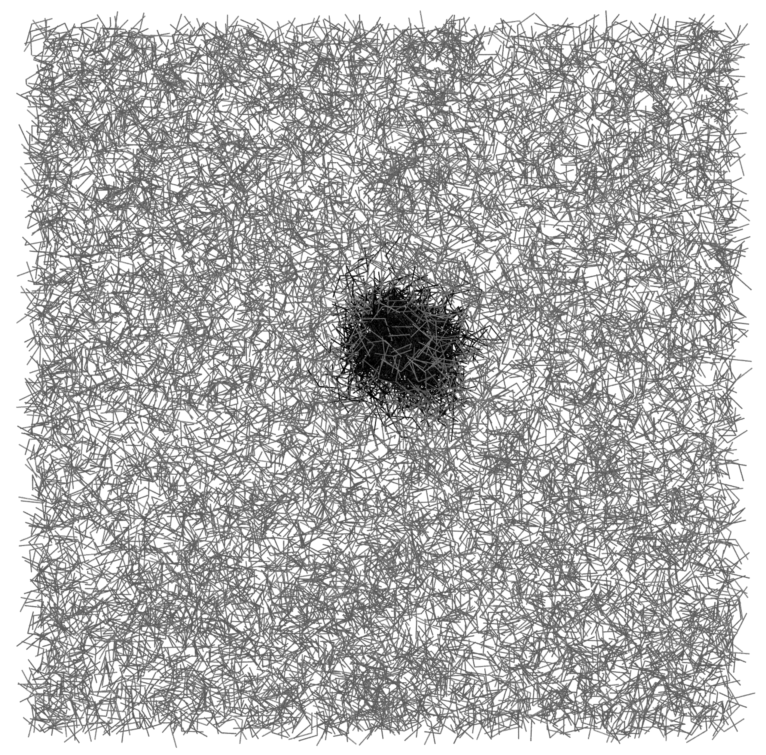
The effect of relabeling may be seen in Figure 2, where snapshots of a single water molecule along the trajectory are displayed before and after relabeling. It is readily seen that the volume spanned by the molecule in the relabeled state is comparable to .
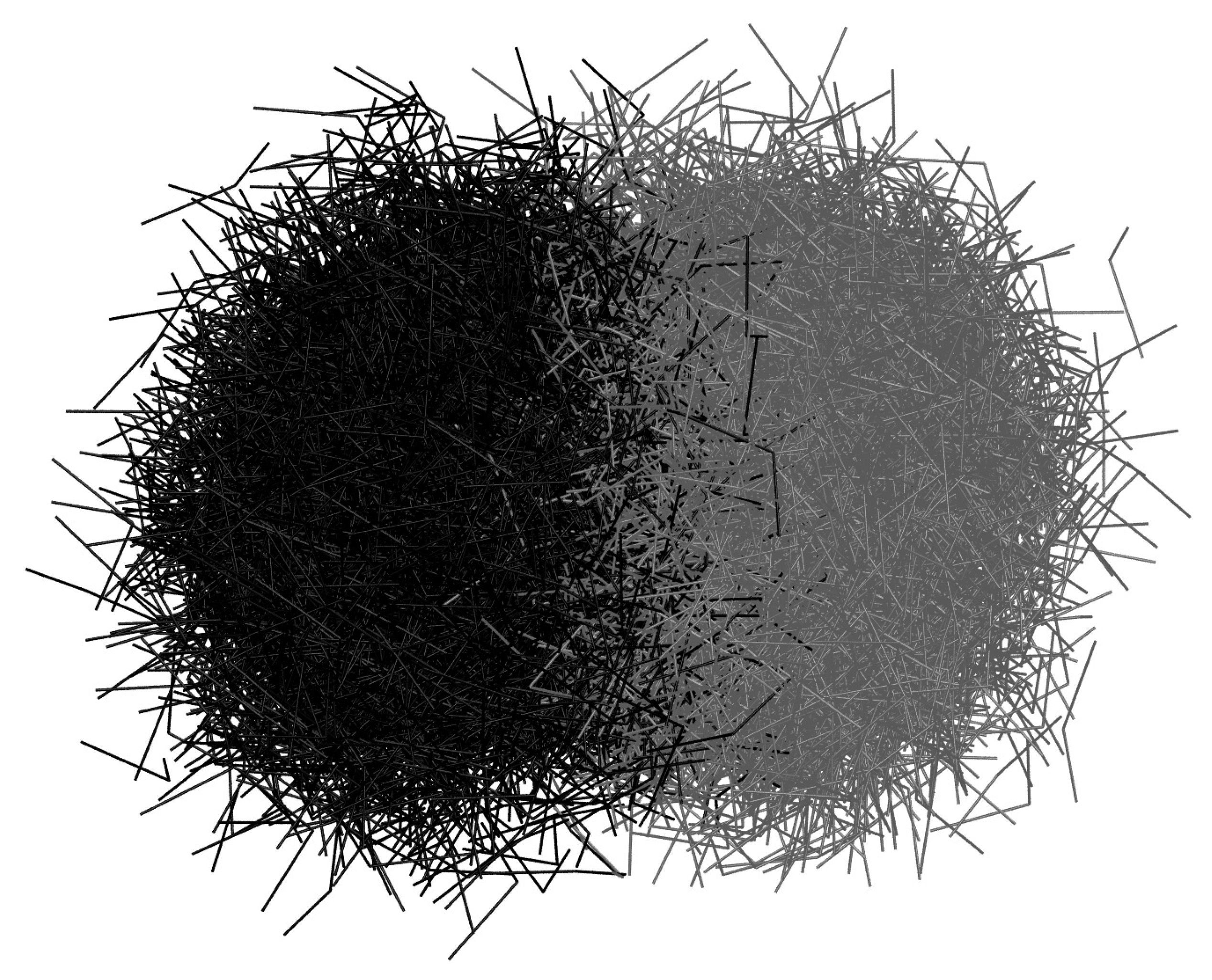
Relabeling of molecules results in moderate overlap of the spaces covered by each molecule. In order to evaluate the extent of the overlap among distributions, we considered the closest (in the reference configuration) relabeled molecules (Figure 3) and computed the average separation of the centers of the distributions (2.99 Å) and the average root mean square deviation along the principal axes of the distributions (1.09 Å).
The distribution of the oxygen atom of each relabeled molecule may be approximated by a three-dimensional Gaussian distribution, allowing the calculation of the overlap integral, defined as the integral of the minimum of the two distributions (centered at 2.99 Å distance and showing a root mean square deviaton of 1.09 Å along the axis connecting the two centers), which amounts to 0.17.
An assessment of the effect of such overlap on the entropy of single-molecule distributions is discussed in the following subsection.
3.2. Single-Molecule Entropy from Single-Molecule Distributions
We have used the formulae reported in the Methods section to estimate the single-molecule entropy for the distributions of all relabeled molecules. In practice, each relabeled molecule has its own localized distribution with associated entropy. The sum of the entropies of the individual distributions is similar, but in general different than the real entropy because the distributions are spread, not disjoint and show some overlap with each other as described above.
We first sorted the neighbours in the reference configuration by their oxygen–oxygen distance, then we considered all pairs of molecules closer than 12 Å, and the list of the first 40 neighbours, i.e., those likely to be more affected by overlap, was retained. For each of these closest neighbours, we have estimated the entropy of the distribution obtained considering each snapshot of the reference molecule and the neighbour as snapshots of the same molecule as detailed in the methods section. The computed entropy of such a pooled ensemble (say for molecule i and j) corresponds to:
In practice, for the normalized sum of two non-overlapping distributions, the entropy will be the mean of the entropy of the two distributions plus a term arising from the two disjoint spaces where the molecule can be found with a probability of a each.
If the distributions are overlapping, then the difference in the entropy with respect to the mean of the two distributions will be lower than and zero if the two distributions are exactly the same.
To assess the effect of overlapping on entropy, ten molecules were selected randomly and for each of their 40 neighbours, the entropy of their disjoint and pooled distributions were computed using the kNN method.
The practical implementation of the kNN method has been thoroughly described previously [38], and the figures we describe in the following are obtained by smooth extrapolation of the entropy to zero kNN distance. All the details and examples are given in the cited reference [38].
The set of snapshots relabeled based on the first snapshot results in a cloud of configurations for each molecule, as shown for two such overlapping distributions in Figure 3. Relabeling of hydrogen atoms is also based on the first snapshot. It is important to keep in mind that, when computing distances between configurations, the labeling of protons should be chosen so as to make the distance shorter. If this is not done, i.e., if the indistinguishability is not taken into account, after the first relabeling, the entropy of the distribution and the overlap are overestimated. Although the spatial overlap of the distributions for neighbouring molecules in the first reference snapshot is not negligible, the entropy difference between pooled and single distributions is almost exactly equal to the term . The apparent contradiction is due to the fact that the different orientations of the molecules and relabeling of protons make the distance from molecules in the pooled set to molecules in their original set shorter than for the other set.
If we take a central molecule and select only the four closest neighbour molecules, the overlap of distributions lowers the computed entropy on average by ; the effect is thus very small.
The configurational entropy expected for the system of randomly distributed indistinguishable molecules in an average volume of Å, where one of the two rotational states (symmetric upon swapping protons) is selected, is , with respect to the 1 M, random orientation standard state.
The entropy computed for the distribution of molecules referenced to the first snapshot is larger than expected (, only incidentally numerically similar to ). The reason why this happens is that the probability density is not uniform but decreases with the distance from the reference molecule.
In the approach presented here, this bias is not, however, relevant because the distances are computed for each molecule along the trajectory relative to the molecule with the same label in the reference configuration and the latter is at the center of the distribution (because molecules are relabeled in order to minimize the distances from molecules in the reference configuration). Close to this position, i.e., in the space sampled by the first nearest neighbours, the density arises almost entirely from molecules which are relabeled according to the reference molecule, and it, therefore, approximates very well the true single particle density.
The mean entropy computed along the trajectory indeed matches within fluctuations in the theoretical value.
3.3. Accuracy
The accuracy of the kNN method applied to translation-rotation and its dependence on the neighbour, number of samples and scaling parameter has been thouroughly reviewed previously [37]. The scheme presented here differs from previous applications in that for each ensemble of molecules, all distances are taken with respect to the single reference snapshot instead of using all pairwise distances among snapshots. To assess the accuracy of this procedure, we choose 100 reference snapshots and 10 molecules from the free water simulation at 310 K, for which the single-molecule entropy is known and equal to the freely rotating molecule at the given concentration of 54.72 M with the choice of one labeling of the hydrogens (−4.695 ) with respect to the 1 M, freely rotating state. For each of the 100 reference snapshots, we optimally relabel all other snapshots and compute for each of the 10 chosen molecules the entropy using the kNN method. The analysis is performed in the realistic scenario of a 500 ns simulation with snapshots taken at 10 ps intervals.
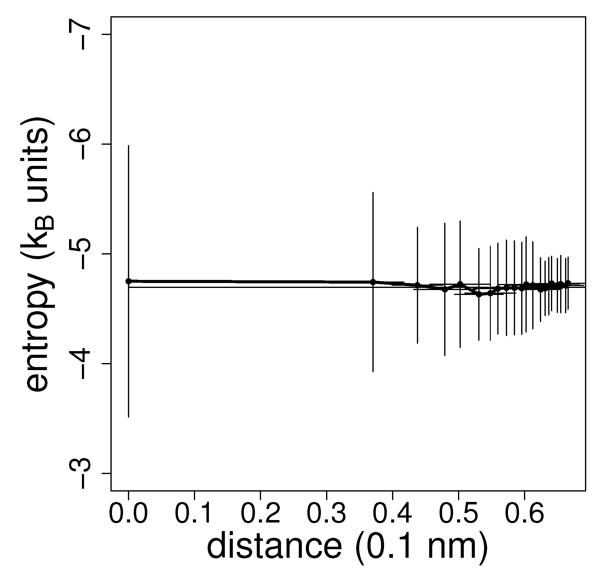
Entropy estimation for a single molecule and for a single reference snapshot is rather noisy depending on the distance to the first nearest neighbours. For this reason, averaging is essential. Figure 4 shows the plot of the average estimated entropy versus the average k-th nearest neighbour distance (increasing with k) and the estimate from extrapolation to zero distance. The variance of the estimated entropy increases with decreasing k in agreement with theoretical estimates [23].
From the figure, the uncertainty of each entropy determination referenced to a single molecule may be assessed.
3.4. Computational Time
The complexity of the Hungarian algorithm as implemented by Knuth [62] is . To assess the actual dependence of the computational time on the increased number of molecules considered for relabeling, we performed 100,000 optimal relabelings for an increasing number (from 80 to 680 in steps of 40) of water molecules. The log–log plot of the running time versus the number of molecules is a straight line with slope 2.272, less than the expected 3, most likely due to the non-random structure of the distance matrix, where each row and column display 4 to 6 distances that are much shorter than all others. The running time of molecule pairwise distance computation and relabeling for two snapshots on a single core of an Intel(R) Core(TM) i7-4900MQ CPU running at 2.80 GHz is s, where n is the number of molecules.
3.5. Application Example: Waters around a Fixed Water Molecule
As an application example, a simulation was run where a water was fixed. The distribution of other water molecules in proximity of the fixed molecule is preferentially oriented so as to form hydrogen bonds. The temperature (310 K in the simulation) results in fluctuations about optimal positions. Since molecules are indexed in each snapshot based on distance from the fixed molecule, the entropy computed for all molecules should increase with their index.
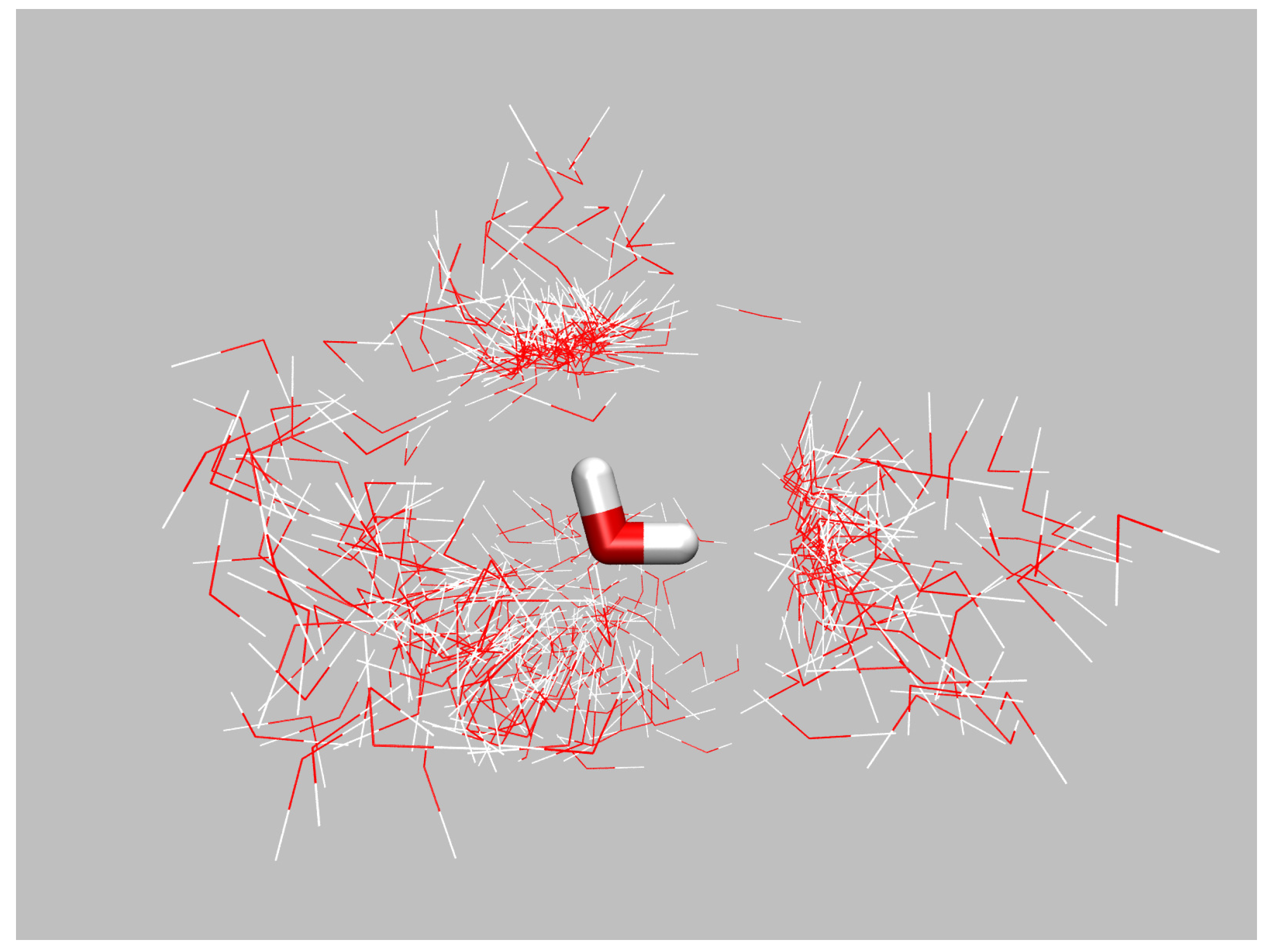
In Figure 5, 100 snapshots along the trajectory of the molecules relabeled according to the four molecules closest to the fixed molecule in the first snapshot, are shown.
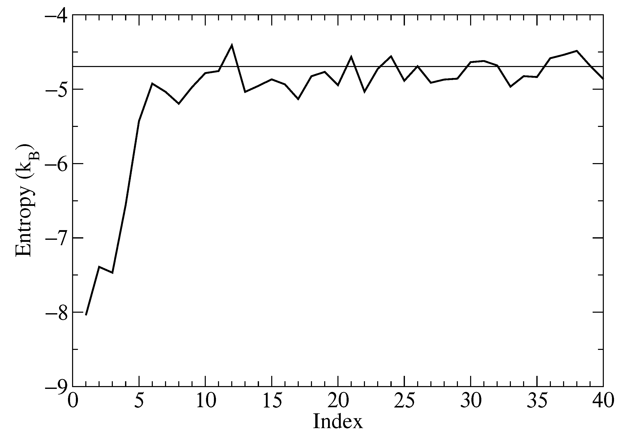
The single-molecule entropy corresponding to each molecule, computed as described in the Materials and Methods and averaged over 200 snapshots, is reported in Figure 6. The reduction in entropy for the four molecules closest to the fixed molecule is apparent. By symmetry, it could be expected that the entropy of the first four molecules should be the same, but in practice, the molecules matched to the closest molecules in the reference snapshot are on average more restricted than more distant ones. This effect is visible in the figure. The entropy computed for the first closest molecules is significantly less than that for more distant molecules for which it approaches the theoretical value for independent molecules at the same concentration with the same symmetry.
Summing up the differences with respect to the independent molecules, for the closest nine molecules, i.e., up to the last molecule with entropy less than for the independent molecules’ case, a value of is obtained corresponding to kcal/mol at 310 K. This value is smaller but similar to the value ( kcal/mol) obtained using SSTMap [19] by difference with respect to the free simulation, for the sum of orientational and translational entropies in a grid of Å centered on the fixed molecule.
4. Conclusions
The estimation of entropy of solvation is a long-standing problem in biomolecular simulations. The indistinguishability of molecules results in theoretical and practical approaches mostly based on distribution functions, which form the standard basis to analyse molecular dynamics simulations of liquids.
Here, we have mapped the problem into a problem where all molecules and their symmetric parts are relabeled in such a way that the global distance from a reference configuration is minimal.
The approach has some distinct advantage in that, after relabeling, molecules display localized distributions, making it possible to analyse global distributions in terms of single molecules. For example, a bound water exchanging with bulk would always likely receive the same label, making the analysis easier. Moreover, in the process of relabeling, the distances from the reference configuration can be used to estimate the entropy of individual molecules, giving a direct measure of restrictions in translational and rotational freedom. For pure water at 310 K, the agreement with the expected theoretical entropy is within 0.04 .
The perspectives opened by the approach are two-fold.
First, the two-molecule entropies and mutual information can be computed in order to use established methods such as the MIE or MIST approach to entropy estimation. The main drawback is that the kNN method, being based on pairwise distances and sorting, is a slow method. Moreover, pairs of molecules are described in a 12-dimensional space, and therefore, the number of snapshots needed to achieve a reasonable resolution is large, in the range of 100,000, which makes the method even slower.
Second, the cost of matching in the Hungarian algorithm defines a metric on the space of configurations (if the cost of matching a molecule is a metric). Such a distance could be used in a kNN approach to estimate the entropy of an ensemble of configurations. The same limitations described above apply here. Both these directions will be explored in future work.
Author Contributions
Conceptualization, F.F. and G.E.; formal analysis: F.F. All authors have read and agreed to the published version of the manuscript.
Funding
This research was funded by the University of Udine grant PRID2017 (Project PRONANO).
Data Availability Statement
All data are reported in the manuscript.
Conflicts of Interest
The authors declare no conflict of interest.
Abbreviations
The following abbreviations are used in this manuscript:
| kNN | k-th nearest neighbour |
| MIE | Mutual information expansion |
| MIST | Maximum information spanning tree |
References
- Gilson, M.K.; Given, J.A.; Bush, B.L.; McCammon, J.A. The statistical-thermodynamic basis for computation of binding affinities: A critical review. Biophys. J. 1997, 72, 1047–1069. [Google Scholar] [CrossRef] [Green Version]
- Roux, B.; Simonson, T. Implicit solvent models. Biophys. Chem. 1999, 78, 1–20. [Google Scholar] [CrossRef]
- Kollman, P.A.; Massova, I.; Reyes, C.; Kuhn, B.; Huo, S.; Chong, L.; Lee, M.; Lee, T.; Duan, Y.; Wang, W.; et al. Calculating structures and free energies of complex molecules: Combining molecular mechanics and continuum models. Acc. Chem. Res. 2000, 33, 889–897. [Google Scholar] [CrossRef]
- Wereszczynski, J.; McCammon, J.A. Statistical mechanics and molecular dynamics in evaluating thermodynamic properties of biomolecular recognition. Q. Rev. Biophys. 2012, 45, 1–25. [Google Scholar] [CrossRef]
- Polyansky, A.A.; Zubac, R.; Zagrovic, B. Estimation of conformational entropy in protein-ligand interactions: A computational perspective. Methods Mol. Biol. 2012, 819, 327–353. [Google Scholar]
- Suarez, D.; Diaz, N. Direct methods for computing single-molecule entropies from molecular simulations. WIREs Comput. Mol. Sci. 2015, 5, 1–26. [Google Scholar] [CrossRef]
- Kassem, S.; Ahmed, M.; El-Sheikh, S.; Barakat, K.H. Entropy in bimolecular simulations: A comprehensive review of atomic fluctuations-based methods. J. Mol. Graph. Model. 2015, 62, 105–117. [Google Scholar] [CrossRef]
- Fogolari, F.; Corazza, A.; Esposito, G. Free energy, enthalpy and entropy from implicit solvent end-point simulations. Front. Mol. Biosci. 2018, 5, 11. [Google Scholar] [CrossRef] [Green Version]
- Beveridge, D.; diCapua, L. Free energy via molecular simulation: Applications to chemical and biomolecular systems. Annu. Rev. Biophys. Chem. 1989, 18, 431–492. [Google Scholar] [CrossRef]
- Zwanzig, R.W. High temperature equation of state by a perturbation method. I. Nonpolar gases. J. Chem. Phys. 1954, 22, 1420–1426. [Google Scholar] [CrossRef]
- Straatsma, T.P.; McCammon, J.A. Multiconfiguration thermodynamic integration. J. Chem. Phys. 1954, 95, 1175–1188. [Google Scholar] [CrossRef]
- Wan, S.; Stote, R.H.; Karplus, M. Calculation of the aqueous solvation energy and entropy, as well as free energy, of simple polar solutes. J. Chem. Phys. 2004, 121, 9539–9548. [Google Scholar] [CrossRef] [PubMed]
- Lazaridis, T. Inhomogeneous fluid approach to solvation thermodynamics. 1. Theory. J. Phys. Chem. B 1998, 102, 3531–3541. [Google Scholar] [CrossRef]
- Lazaridis, T. Inhomogeneous fluid approach to solvation thermodynamics. 2. Applications to simple fluids. J. Phys. Chem. B 1998, 102, 3542–3550. [Google Scholar] [CrossRef]
- Young, T.; Abel, R.; Kim, B.; Berne, B.J.; Friesner, R.A. Motifs for molecular recognition exploiting hydrophobic enclosure in protein-ligand binding. Proc. Natl. Acad. Sci. USA 2007, 104, 808–813. [Google Scholar] [CrossRef] [PubMed] [Green Version]
- Abel, R.; Young, T.; Farid, R.; Berne, B.J.; Friesner, R.A. Role of the active-site solvent in the thermodynamics of factor Xa ligand binding. J. Am. Chem. Soc. 2008, 130, 2817–2831. [Google Scholar] [CrossRef] [Green Version]
- Nguyen, C.N.; Young, T.K.; Gilson, M.K. Grid inhomogeneous solvation theory: Hydration structure and thermodynamics of the miniature receptor cucurbit[7]uril. J. Chem. Phys. 2012, 137, 044101. [Google Scholar] [CrossRef] [PubMed] [Green Version]
- Ramsey, S.; Nguyen, C.; Salomon-Ferrer, R.; Walker, R.C.; Gilson, M.K.; Kurtzman, T. Solvation thermodynamic mapping of molecular surfaces in AmberTools: GIST. J. Comput. Chem. 2016, 37, 2029–2037. [Google Scholar] [CrossRef] [Green Version]
- Haider, K.; Cruz, A.; Ramsey, S.; Gilson, M.K.; Kurtzman, T. Solvation structure and thermodynamic mapping (SSTMap): An open-source, flexible package for the analysis of water in molecular dynamics trajectories. J. Chem. Theory Comput. 2018, 14, 418–425. [Google Scholar] [CrossRef]
- Ross, G.A.; Bodnarchuk, M.S.; Essex, J.W. Water sites, networks, and free energies with Grand Canonical Monte Carlo. J. Am. Chem. Soc. 2015, 137, 14930–14943. [Google Scholar] [CrossRef] [Green Version]
- Kovalenko, A. Three-dimensional RISM theory for molecular liquids and solid-liquid interfaces. In Molecular Theory of Solvation; Hirata, F., Ed.; Kluwer Academic Publishers: Dordrecht, The Netherlands, 2003; Chapter 4; pp. 169–275. [Google Scholar]
- Bodnarchuk, M.S. Water, water, everywhere... It’s time to stop and think. Drug Discov. Today 2016, 21, 1139–1146. [Google Scholar] [CrossRef]
- Singh, H.; Misra, N.; Hnizdo, V.; Fedorowicz, A.; Demchuk, E. Nearest neighbor estimate of entropy. Am. J. Math. Manag. Sci. 2003, 23, 301–321. [Google Scholar] [CrossRef]
- Hnizdo, V.; Darian, E.; Fedorowicz, A.; Demchuk, E.; Li, S.; Singh, H. Nearest-neighbor nonparametric method for estimating the configurational entropy of complex molecules. J. Comput. Chem. 2007, 28, 655–668. [Google Scholar] [CrossRef]
- Numata, J.; Wan, M.; Knapp, E.W. Conformational entropy of biomolecules: Beyond the quasi-harmonic approximation. Genome Inform. 2007, 18, 192–205. [Google Scholar]
- Hnizdo, V.; Tan, J.; Killian, B.J.; Gilson, M.K. Efficient calculation of configurational entropy from molecular simulations by combining the mutual-information expansion and nearest-neighbor methods. J. Comput. Chem. 2008, 29, 1605–1614. [Google Scholar] [CrossRef] [Green Version]
- Wang, L.; Abel, R.; Friesner, R.A.; Berne, B.J. Thermodynamic properties of liquid water: An application of a nonparametric approach to computing the entropy of a neat fluid. J. Chem. Theory Comput. 2009, 5, 1462–1473. [Google Scholar] [CrossRef] [Green Version]
- Misra, N.; Singh, H.; Hnizdo, V. Nearest neighbor estimates of entropy for multivariate circular distributions. Entropy 2010, 12, 578–590. [Google Scholar] [CrossRef] [Green Version]
- Mukherjee, A. Entropy Balance in the Intercalation Process of an Anti-Cancer Drug Daunomycin. J. Phys. Chem. Lett. 2011, 2, 3021–3026. [Google Scholar] [CrossRef]
- Fenley, A.T.; Killian, B.J.; Hnizdo, V.; Fedorowicz, A.; Sharp, D.S.; Gilson, M.K. Correlation as a determinant of configurational entropy in supramolecular and protein systems. J. Phys. Chem. B 2014, 118, 6447–6455. [Google Scholar] [CrossRef] [Green Version]
- Nguyen, C.N.; Cruz, A.; Gilson, M.K.; Kurtzman, T. Thermodynamics of water in an enzyme active site: Grid-based hydration analysis of coagulation factor Xa. J. Chem. Theory Comput. 2014, 10, 2769–2780. [Google Scholar] [CrossRef]
- Fogolari, F.; Corazza, A.; Fortuna, S.; Soler, M.A.; VanSchouwen, B.; Brancolini, G.; Corni, S.; Melacini, G.; Esposito, G. Distance-based configurational entropy of proteins from molecular dynamics simulations. PLoS ONE 2015, 10, e0132356. [Google Scholar] [CrossRef] [PubMed] [Green Version]
- Huggins, D.J. Comparing distance metrics for rotation using the k-nearest neighbors algorithm for entropy estimation. J. Comput. Chem. 2014, 35, 377–385. [Google Scholar] [CrossRef] [PubMed] [Green Version]
- Huggins, D.J. Estimating translational and orientational entropies using the k-nearest neighbors algorithm. J. Chem. Theory Comput. 2014, 10, 3617–3625. [Google Scholar] [CrossRef] [Green Version]
- Huggins, D.J. Quantifying the entropy of binding for water molecules in protein cavities by computing correlations. Biophys. J. 2014, 35, 377–385. [Google Scholar] [CrossRef] [Green Version]
- Sasikala, W.D.; Mukherjee, A. Single water entropy: Hydrophobic crossover and application to drug binding. J. Phys. Chem. B 2014, 118, 10553–10564. [Google Scholar] [CrossRef]
- Fogolari, F.; Dongmo Foumthuim, C.J.; Fortuna, S.; Soler, M.A.; Corazza, A.; Esposito, G. Accurate Estimation of the Entropy of Rotation-Translation Probability Distributions. J. Chem. Theory Comput. 2016, 12, 1–8. [Google Scholar] [CrossRef]
- Fogolari, F.; Esposito, G.; Tidor, B. Entropy of two-molecule correlated translational-rotational motions using the kth nearest neighbor method. J. Chem. Theory Comput. 2021, 17, 3039–3051. [Google Scholar] [CrossRef]
- Huggins, D.J. Studying the role of cooperative hydration in stabilizing folded protein states. J. Struct. Biol. 2016, 196, 394–406. [Google Scholar] [CrossRef] [Green Version]
- Irwin, B.W.J.; Huggins, D.J. On the accuracy of one- and two-particle solvation entropies. J. Chem. Phys. 2017, 146, 194111. [Google Scholar] [CrossRef] [Green Version]
- Heinz, L.P.; Grubmüller, H. Computing spatially resolved rotational hydration entropies from atomistic simulations. J. Chem. Theory Comput. 2020, 16, 108–118. [Google Scholar] [CrossRef] [Green Version]
- Heinz, L.P.; Grubmüller, H. Per|Mut: Spatially resolved hydration entropies from atomistic simulations. J. Chem. Theory Comput. 2021, 17, 2090–2091. [Google Scholar] [CrossRef] [PubMed]
- Killian, B.J.; Yundenfreund Kravitz, J.; Gilson, M.K. Extraction of configurational entropy from molecular simulations via an expansion approximation. J. Chem. Phys. 2007, 127, 024107. [Google Scholar] [CrossRef] [PubMed] [Green Version]
- King, B.M.; Tidor, B. MIST: Maximum Information Spanning Trees for dimension reduction of biological data sets. Bioinformatics 2009, 25, 1165–1172. [Google Scholar] [CrossRef] [Green Version]
- King, B.M.; Silver, N.W.; Tidor, B. Efficient calculation of molecular configurational entropies using an information theoretic approximation. J. Phys. Chem. B 2012, 116, 2891–2904. [Google Scholar] [CrossRef] [Green Version]
- Silver, N.W.; King, B.M.; Nalam, M.N.L.; Cao, H.; Ali, A.; Kiran Kumar Reddy, G.S.; Rana, T.M.; Schiffer, C.A.; Tidor, B. Efficient Computation of Small-Molecule Configurational Binding Entropy and Free Energy Changes by Ensemble Enumeration. J. Chem. Theory Comput. 2013, 9, 5098–5115. [Google Scholar] [CrossRef] [Green Version]
- Fenley, A.T.; Muddana, H.S.; Gilson, M.K. EEntropy–enthalpy transduction caused by conformational shifts can obscure the forces driving protein–ligand binding. Proc. Natl. Acad. Sci. USA 2012, 109, 20006–20011. [Google Scholar] [CrossRef] [PubMed] [Green Version]
- Fleck, M.; Polyansky, A.A.; Zagrovic, B. PARENT: A parallel software suite for the calculation of configurational entropy in biomolecular systems. J. Chem. Theory Comput. 2016, 12, 2055–2065. [Google Scholar] [CrossRef]
- Fogolari, F.; Maloku, O.; Dongmo Foumthuim, C.J.; Corazza, A.; Esposito, G. PDB2ENTROPY and PDB2TRENT: Conformational and translational-rotational entropy from molecular ensembles. J. Chem. Inf. Model. 2018, 58, 1319–1324. [Google Scholar] [CrossRef]
- Dongmo Foumthuim, C.J.; Corazza, A.; Berni, R.; Esposito, G.; Fogolari, F. Dynamics and Thermodynamics of Transthyretin Association from Molecular Dynamics Simulations. BioMed Res. Int. 2018, 2018, 7480749. [Google Scholar] [CrossRef] [Green Version]
- Lazaridis, T.; Karplus, M. Orientational correlations and entropy in liquid water. J. Chem. Phys. 1996, 105, 4294–4316. [Google Scholar] [CrossRef]
- Singer, A. Maximum entropy formulation of the Kirkwood superposition approximation. J. Chem. Phys. 2004, 121, 3657–3666. [Google Scholar] [CrossRef] [PubMed]
- Wallace, D.C. On the role of density fluctuations in the entropy of a fluid. J. Chem. Phys. 1987, 87, 2281–2284. [Google Scholar] [CrossRef]
- Tan, Z.; Gallicchio, E.; Lapelosa, M.; Levy, R.M. Theory of binless multi-state free energy estimation with applications to protein-ligand binding. J. Chem. Phys. 2012, 136, 144102. [Google Scholar] [CrossRef] [Green Version]
- Zhang, B.W.; Cui, D.; Matubayasi, N.; Levy, R.M. The Excess Chemical Potential of Water at the Interface with a Protein from End Point Simulations. J. Phys. Chem. B 2018, 122, 4700–4707. [Google Scholar] [CrossRef]
- Reinhard, F.; Grubmüller, H. Estimation of absolute solvent and solvation shell entropies via permutation reduction. J. Chem. Phys. 2007, 126, 014102. [Google Scholar] [CrossRef]
- Kozachenko, L.F.; Leonenko, N.N. Sample estimates of entropy of a random vector. Probl. Inf. Transm. 1987, 23, 95–101. [Google Scholar]
- Huynh, D.Q. Metrics for 3D rotations: Comparison and analysis. J. Math. Imaging Vis. 2009, 35, 155–164. [Google Scholar] [CrossRef]
- Ò Searcòid, M. Metric Spaces; Springer: London, UK, 2007. [Google Scholar]
- Miles, R.E. On random rotations in R3. Biometrika 1965, 52, 636–639. [Google Scholar] [CrossRef]
- Kuhn, H.W. The hungarian method for the assignment problem. Naval Res. Log. Quart. 1955, 2, 83–97. [Google Scholar] [CrossRef] [Green Version]
- Knuth, D.E. Stanford GraphBase; ACM Press: New York, NY, USA, 1986. [Google Scholar]
- Jorgensen, W.L.; Chandrasekhar, J.; Madura, J.D.; Impey, R.W.; Klein, M.L. Comparison of simple potential functions for simulating liquid water. J. Chem. Phys. 1983, 79, 926–935. [Google Scholar] [CrossRef]
- Martyna, G.; Tobias, D.; Klein, M. Constant pressure molecular dynamics algorithms. J. Chem. Phys. 1994, 101, 4177–4189. [Google Scholar] [CrossRef]
- Feller, S.; Zhang, Y.; Pastor, R.; Brooks, B. Constant pressure molecular dynamics simulation: The Langevin piston method. J. Chem. Phys. 1995, 103, 4613–4621. [Google Scholar] [CrossRef]
- Miyamoto, S.; Kollman, P.A. Settle: An analytical version of the SHAKE and RATTLE algorithm for rigid water models. J. Comput. Chem. 1992, 13, 952–962. [Google Scholar] [CrossRef]
- Kale, L.; Skeel, R.; Bhandarkar, M.; Brunner, R.; Gursoy, A.; Krawetz, N.; Phillips, J.; Shinozaki, A.; Varadarajan, K.; Schulten, K. NAMD2: Greater scalability for parallel molecular dynamics. J. Comput. Phys. 1999, 151, 283–312. [Google Scholar] [CrossRef]
- Humphrey, W.; Dalke, A.; Schulten, K. VMD Visual Molecular Dynamics. J. Mol. Graph. 1996, 14, 33–38. [Google Scholar] [CrossRef]
Figure 1.
A sketch of some steps of the Hungarian algorithm. (A) The initial cost matrix (e.g., distances among five water molecules in the sample and reference configuration) is shown. The minima in each row are underlined and subtracted from the relative rows to yeld a new cost matrix. (B) The minimima different from zero in each column are underlined and subtracted from each column to yeld a new cost matrix. (C) In the new cost matrix, some “matching” zeroes (shown in bold) match one column and one row uniquely. Non-matching zeroes are underlined. Paths starting and ending on an underlined zero and alternating matching and non-matching zeroes, such as the one highlighted by the thick dashed line, are sought and new matching zeroes are chosen. If no such path exists, the algorithm performs subtractions and additions to the columns and the rows which do not alter the solution and create new paths [62]. This step is iterated until completion, to yeld a new matrix with a unique chosen zero on each row and each column. (D) The set of chosen zeroes in the matrix (one per row and column) is the sought assignment, i.e., in this example, W1 in the sample is assigned the label W5, W2 is assigned the label W3, etc.

Figure 2.
10,000 snapshots for a single molecule from the dynamics are shown in gray and 1000 snapshots in black after relabeling.
Figure 2.
10,000 snapshots for a single molecule from the dynamics are shown in gray and 1000 snapshots in black after relabeling.

Figure 3.
10,000 snapshots for two neighbouring relabeled molecules from the dynamics are shown in gray and black, respectively.
Figure 3.
10,000 snapshots for two neighbouring relabeled molecules from the dynamics are shown in gray and black, respectively.

Figure 4.
The average estimated entropy (and its extrapolation to zero distance) is plotted against the average distance to the first 20 nearest neighbours with error bars on both distance and entropy estimate. The vertical error bars are equal to the standard deviations of the entropy estimate drawn for each individual molecule in a single snapshot from the first 20 neighbours in all other snapshots.

Figure 5.
100 snapshots along a 10 ns trajectory of the molecules matched to the four molecules closest to the fixed water in the reference snapshot. Oxygen atoms are shown in red and hydrogen atoms in white.
Figure 5.
100 snapshots along a 10 ns trajectory of the molecules matched to the four molecules closest to the fixed water in the reference snapshot. Oxygen atoms are shown in red and hydrogen atoms in white.

Figure 6.
The entropy of the relabeled molecules (continuous line) indexed based on the distance from the fixed molecule. The entropy corresponding to the non-interacting symmetric molecules is shown by the broken line.
Figure 6.
The entropy of the relabeled molecules (continuous line) indexed based on the distance from the fixed molecule. The entropy corresponding to the non-interacting symmetric molecules is shown by the broken line.

Publisher’s Note: MDPI stays neutral with regard to jurisdictional claims in published maps and institutional affiliations. |
© 2021 by the authors. Licensee MDPI, Basel, Switzerland. This article is an open access article distributed under the terms and conditions of the Creative Commons Attribution (CC BY) license (https://creativecommons.org/licenses/by/4.0/).
Share and Cite
MDPI and ACS Style
Fogolari, F.; Esposito, G. Optimal Relabeling of Water Molecules and Single-Molecule Entropy Estimation. Biophysica 2021, 1, 279-296. https://0-doi-org.brum.beds.ac.uk/10.3390/biophysica1030021
AMA Style
Fogolari F, Esposito G. Optimal Relabeling of Water Molecules and Single-Molecule Entropy Estimation. Biophysica. 2021; 1(3):279-296. https://0-doi-org.brum.beds.ac.uk/10.3390/biophysica1030021
Chicago/Turabian StyleFogolari, Federico, and Gennaro Esposito. 2021. "Optimal Relabeling of Water Molecules and Single-Molecule Entropy Estimation" Biophysica 1, no. 3: 279-296. https://0-doi-org.brum.beds.ac.uk/10.3390/biophysica1030021