The Tap-Length Associated with the Blind Adaptive Equalization/Deconvolution Problem  ^†

Abstract

The step-size parameter and the equalizer’s tap length are the system parameters in the blind adaptive equalization design. Choosing a large step-size parameter causes the equalizer to converge faster compared with applying a smaller value for the step size parameter. However, a higher step-size parameter leaves the system with a higher residual inter-symbol-interference (ISI) than does a lower step-size parameter. The equalizer’s tap length should be set large enough to compensate for the channel distortions. However, since the channel parameters are unknown, the required equalizer’s tap length is also unknown. The system parameters are usually designed via simulation trials, in such a way that the equalizer’s performance from the residual ISI point of view reaches a system desired residual ISI level. Recently, a closed-form approximated expression was derived for the residual ISI as a function of the system parameters, input sequence statistics and channel power. This expression was obtained under the assumption having a value for the equalizer’s tap length that is sufficient to compensate for the channel distortions. Based on this approximated expression, the outcome from the step-size parameter multiplied by the equalizer’s tap length can be derived when the residual ISI is given. By choosing a step-size parameter, we automatically have also the value for the equalizer’s tap length which might now not be large enough to compensate for the channel distortions and thus leaving the system with a higher residual ISI than the required one. In this work, we derive an expression that sets a condition on the equalizer’s tap length based on the input sequence statistics, on the chosen equalizer’s characteristics and required residual ISI. In addition, highlights are supplied on how to set the equalizer’s tap length for different channel cases based on this new derived expression. The findings are accompanied by simulation results.

1. Introduction

In this work we consider the blind adaptive equalization (blind adaptive deconvolution) problem [1,2,3,4,5,6,7,8,9,10,11,12,13,14,15,16,17,18,19]. For a blind adaptive equalizer, the system designer needs to know how to choose correctly the step-size parameter and the equalizer’s tap length in order to obtain a system required residual inter-symbol-interference (ISI). According to [1], a higher value for the step-size parameter leads the equalizer entering the convergence state faster than for a lower step-size parameter. However, a higher value for the step-size parameter will leave the system with a higher residual ISI compared with a lower value for the step-size parameter [1]. A higher residual ISI may lead to a higher symbol error rate [20] which may no longer answer on the system’s requirements. In addition, a too high value for the step-size parameter may lead the equalizer to disconverge. The equalizer’s tap length should be set large enough to compensate for the channel distortions. Nevertheless, since the channel characteristics are practically unknown to the system designer, the required equalizer’s tap length is also unknown. It could be thought that choosing a very large value for the equalizer’s tap length is the right thing to do. However, according to [1], setting the value for the equalizer’s tap length too high, leads the system to a higher residual ISI than for setting the equalizer’s tap length with a lower value but with a value which still can compensate for the channel distortions. Usually, the step-size parameter and the equalizer’s tap length are obtained via simulation trials where the whole system with the equalizer is simulated. Obviously, the simulation trials waste a lot of time in the general system design. Recently [1,21], a closed-form approximated expression was derived for the achievable residual ISI case that depends on the step-size parameter, equalizer’s tap length, input signal statistics, signal-to-noise ratio (SNR), the chosen equalization method and channel power. This closed-form approximated expression for the residual ISI is applicable for blind adaptive equalizers where the error signal that participates in the update mechanism of the equalizer’s coefficients is a polynomial function of order up to three of the equalized sequence as it is in the case of Godard’s [2] algorithm. Based on this closed-form approximated expression for the residual ISI, the system designer has on hand the value for the step-size parameter multiplied by the equalizer’s tap length for a given residual ISI level. Both the closed-form approximated expressions for the residual ISI in [1,21] assumed to have a value for the equalizer’s tap length that is sufficient to compensate for the channel distortions. Thus, having the outcome of the step-size parameter multiplied by the equalizer’s tap length for a given residual ISI level is not enough for setting practical values for both the step-size parameter and equalizer’s tap length since by setting a high value for the step-size parameter for fast convergence might obtain to a value for the equalizer’s tap length that might not be able anymore to compensate for the channel distortions. In this work, we solve the problem of how to set correctly the equalizer’s tap length based on a new derived expression that sets a condition on the equalizer’s tap length. This new expression is based on the input sequence statistics, on the chosen equalizer’s characteristics and required residual ISI and is applicable for blind adaptive equalizer’s where the error signal that participates in the update mechanism of the equalizer’s coefficients is a polynomial function of order up to three of the equalized sequence. Simulation results confirm our findings.

2. Methods

In this section, we present the condition on the equalizer’s tap-length for the noiseless case.

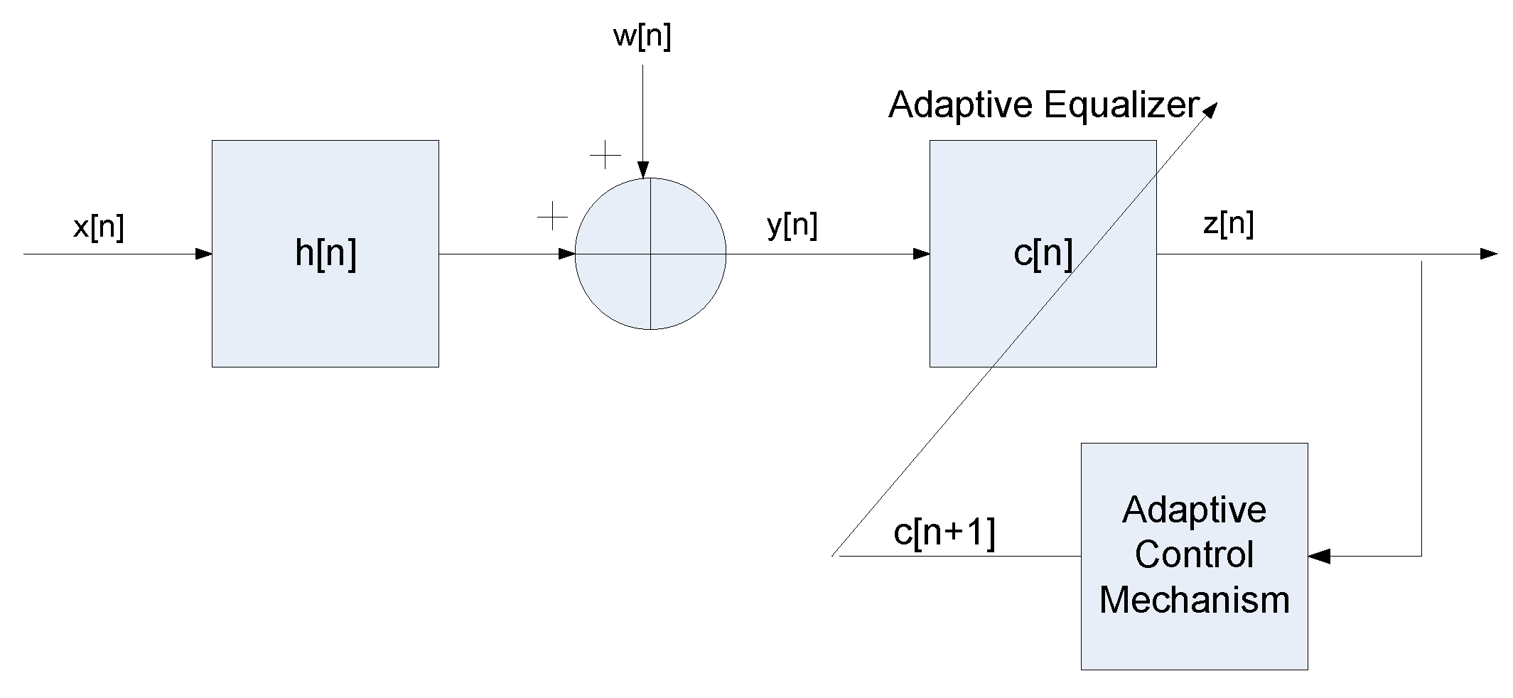
Let us consider the following system (Figure 1 recalled from [22]), where we make the following assumptions according to [22]:

• The input sequence $x\left[n\right]$ can be written as $x\left[n\right]=x_r\left[n\right]+j{x}_i\left[n\right]$ where $x_r\left[n\right]$ and $x_i\left[n\right]$ are the real and imaginary parts of $x\left[n\right]$ respectively. $x_r\left[n\right]$ and $x_i\left[n\right]$ are independent, $E\left[x\left[n\right]x^{*}\left[n\right]\right]={\sigma }_x^2$ and $E\left[x\right[n\left]\right]=0$ (where $E\left[\right(·\left)\right]$ stands for the expectation operator on $(·)$ and ${\left(\right)}^{*}$ is the conjugate operation on ()). In addition: $E\left[x_i^2\left[n\right]\right]={\sigma }_{x_i}^2$, $E\left[x_r^2\left[n\right]\right]={\sigma }_{x_r}^2$, $E\left[x_i^G\left[n\right]\right]=E\left[x_r^G\left[n\right]\right]$ where G is a positive and even integer.
• The unknown channel $h\left[n\right]$ is a possibly nonminimum phase linear time-invariant filter in which the transfer function has no “deep zeros”; namely, the zeros lie sufficiently far from the unit circle.
• The filter $c\left[n\right]$ is a tap-delay line.
• $w\left[n\right]=0$

The equalized output sequence can be written as:

$$z\left[n\right]=y\left[n\right]\ast c\left[n\right]=\left(x\left[n\right]\ast h\left[n\right]\right)\ast c\left[n\right]=x\left[n\right]\ast \left(\delta \left[n\right]+\xi \left[n\right]\right)=x\left[n\right]+x\left[n\right]\ast \xi \left[n\right]=x\left[n\right]+p\left[n\right]$$

(1)

with

$$p\left[n\right]=x\left[n\right]\ast \xi \left[n\right];h\left[n\right]\ast c\left[n\right]=\delta \left[n\right]+\xi \left[n\right]$$

(2)

where “∗” stands for the convolutional operation, $\xi \left[n\right]$ stands for the difference (error) between the ideal and the used value for $c\left[n\right]$ following (3) and $\delta$ is the Kronecker delta function. The equalizer’s coefficients are updated according to [23]:

$$\underline{c}[n+1]=\underline{c}\left[n\right]-\mu \frac{\partial F\left[n\right]}{\partial z\left[n\right]}{\underline{y}}^{*}\left[n\right]$$

(3)

where $\mu$ is the step-size parameter, $F\left[n\right]$ is the cost function and $\underline{c}\left[n\right]$ is the equalizer vector where the input vector is $\underline{y}\left[n\right]={[y\left[n\right]...y[n-N+1]]}^T$. The operator ${\left(\right)}^T$ denotes for transpose of the function () and N is the equalizer’s tap length. In [1], a closed-form approximated expression was derived for the residual inter-symbol-interference (ISI) applicable for a blind adaptive equalizer where the cost function $F\left[n\right]$ is a polynomial function of the equalized output sequence of order up to three:

$$ISI=10{log}_{10}\left(m_p\right)-10{log}_{10}\left({\sigma }_{x_r}^2\right)$$

(4)

where $E\left[p_r^2\left[n\right]\right]=m_p$, ($p\left[n\right]=p_r\left[n\right]+j{p}_i\left[n\right]$) and $m_p$ is obtained by:

$$\begin{array}{c}{m}_p=min\left[So{l}_1^{m{p}_1},So{l}_2^{m{p}_1}\right]forSo{l}_1^{m{p}_1}>0andSo{l}_2^{m{p}_1}>0\\ or\\ m_p=max\left[So{l}_1^{m{p}_1},So{l}_2^{m{p}_1}\right]forSo{l}_1^{m{p}_1}·So{l}_2^{m{p}_1}<0\\ where\\ So{l}_1^{m{p}_1}=\frac{-B_1+\sqrt{B_1^2-4A_1{C}_{1}B}}{2A_1};So{l}_2^{m{p}_1}=\frac{-B_1-\sqrt{B_1^2-4A_1{C}_{1}B}}{2A_1}\end{array}$$

(5)

$$\begin{array}{c}{A}_1=\left(B\left(45{\sigma }_{x_r}^2{a}_3^2+18{\sigma }_{x_r}^2{a}_3{a}_{12}+6a_1{a}_3+9{\sigma }_{x_r}^2{a}_{12}^2+2a_1{a}_{12}\right)-2\left(3a_3+a_{12}\right)\right)\hfill \\ B_1=\left(B\left(12{\left({\sigma }_{x_r}^2\right)}^2{a}_3{a}_{12}+6{\left({\sigma }_{x_r}^2\right)}^2{a}_{12}^2+12{\sigma }_{x_r}^2{a}_1{a}_3+4{\sigma }_{x_r}^2{a}_1{a}_{12}+a_1^2+15E\left[x_r^4\right]a_3^2+\right.\right.\hfill \\ \left.\left.2E\left[x_r^4\right]a_3{a}_{12}+E\left[x_r^4\right]a_{12}^2\right)-2\left(a_1+3{\sigma }_{x_r}^2{a}_3+{\sigma }_{x_r}^2{a}_{12}\right)\right)\hfill \\ C_1=\left(2{\left({\sigma }_{x_r}^2\right)}^2{a}_1{a}_{12}+{\sigma }_{x_r}^2{a}_1^2+2E\left[x_r^4\right]{\sigma }_{x_r}^2{a}_3{a}_{12}+E\left[x_r^4\right]{\sigma }_{x_r}^2{a}_{12}^2+2E\left[x_r^4\right]a_1{a}_3+E\left[x_r^6\right]a_3^2\right)\hfill \\ B=\mu N{\sigma }_x^2\sum _{k=0}^{k=R-1}{\left|h_k\left[n\right]\right|}^2\hfill \end{array}$$

(6)

R is the channel length, $x_r=x_r\left[n\right]$ and $a_1$, $a_{12}$, $a_3$ are properties of the chosen equalizer and found by:

$$Re\left(\frac{\partial F\left(n\right)}{\partial z\left(n\right)}\right)=\left(a_1\left(z_r\right)+a_3{\left(z_r\right)}^3+a_{12}\left(z_r\right){\left(z_i\right)}^2\right)$$

(7)

where $Re(·)$ is the real part of $(·)$ and $z_r$, $z_i$ are the real and imaginary parts of the equalized output $z\left[n\right]$ respectively. In this paper we use Godard’s algorithm [2]. Thus we have:

$$\frac{\partial F\left[n\right]}{\partial z\left[n\right]}=\left({\left|z\left[n\right]\right|}^2-\frac{E\left[{\left|x\left[n\right]\right|}^4\right]}{E\left[{\left|x\left[n\right]\right|}^2\right]}\right)z\left[n\right]$$

(8)

where $|\left(\right)|$ stands for the absolute value of (). Please note that for Godard’s algorithm [2] we have that:

$$a_3=a_{12}=1;a_3=-\frac{E\left[{\left|x\left[n\right]\right|}^4\right]}{E\left[{\left|x\left[n\right]\right|}^2\right]}$$

(9)

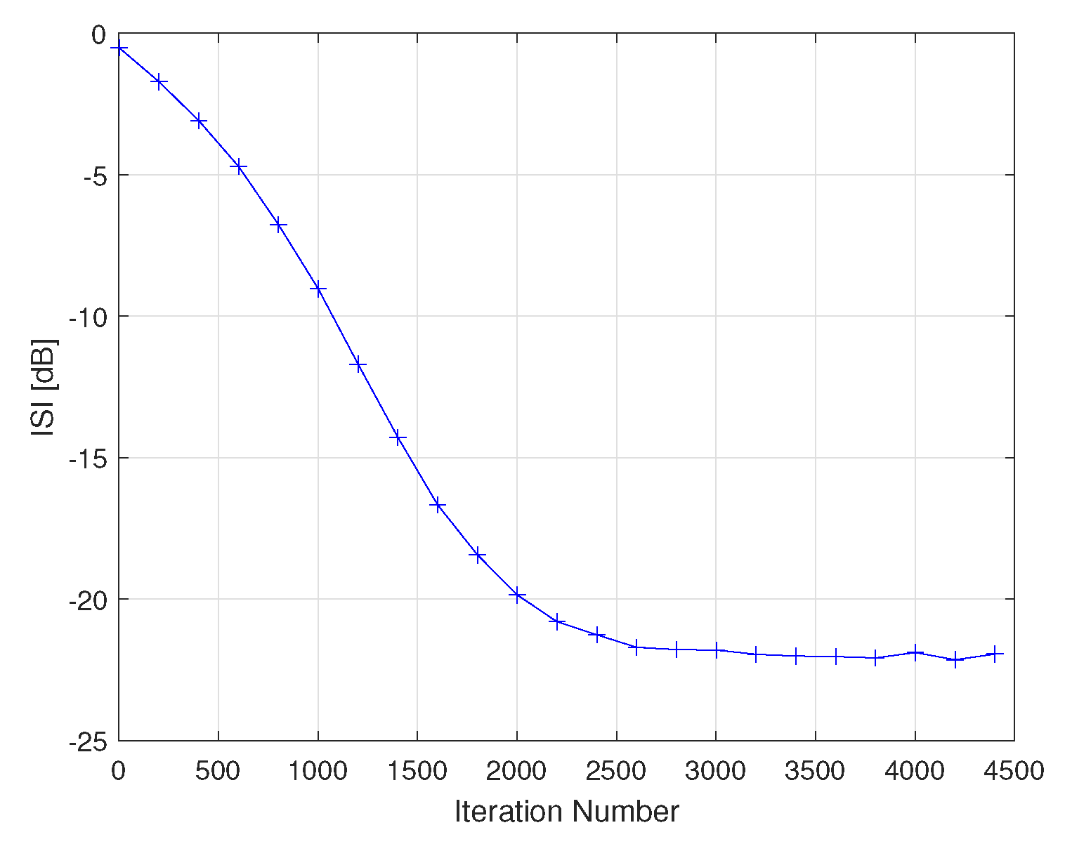
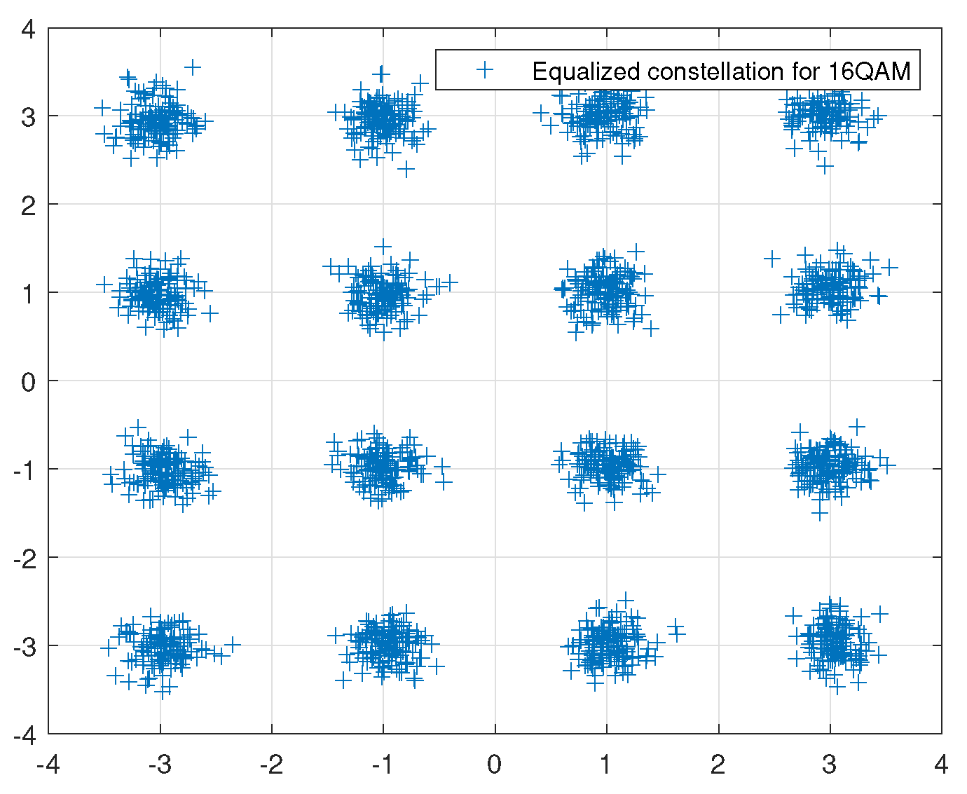
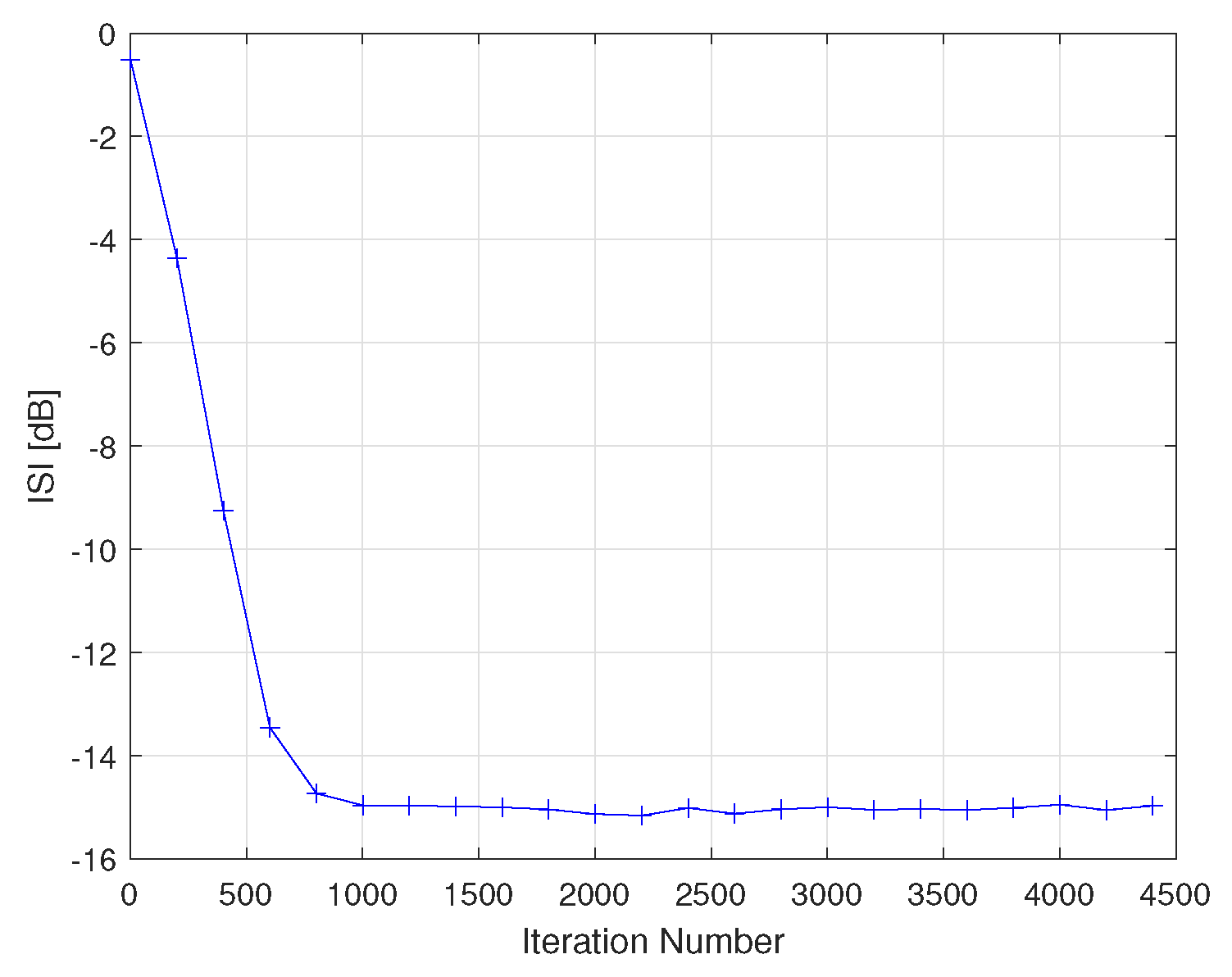
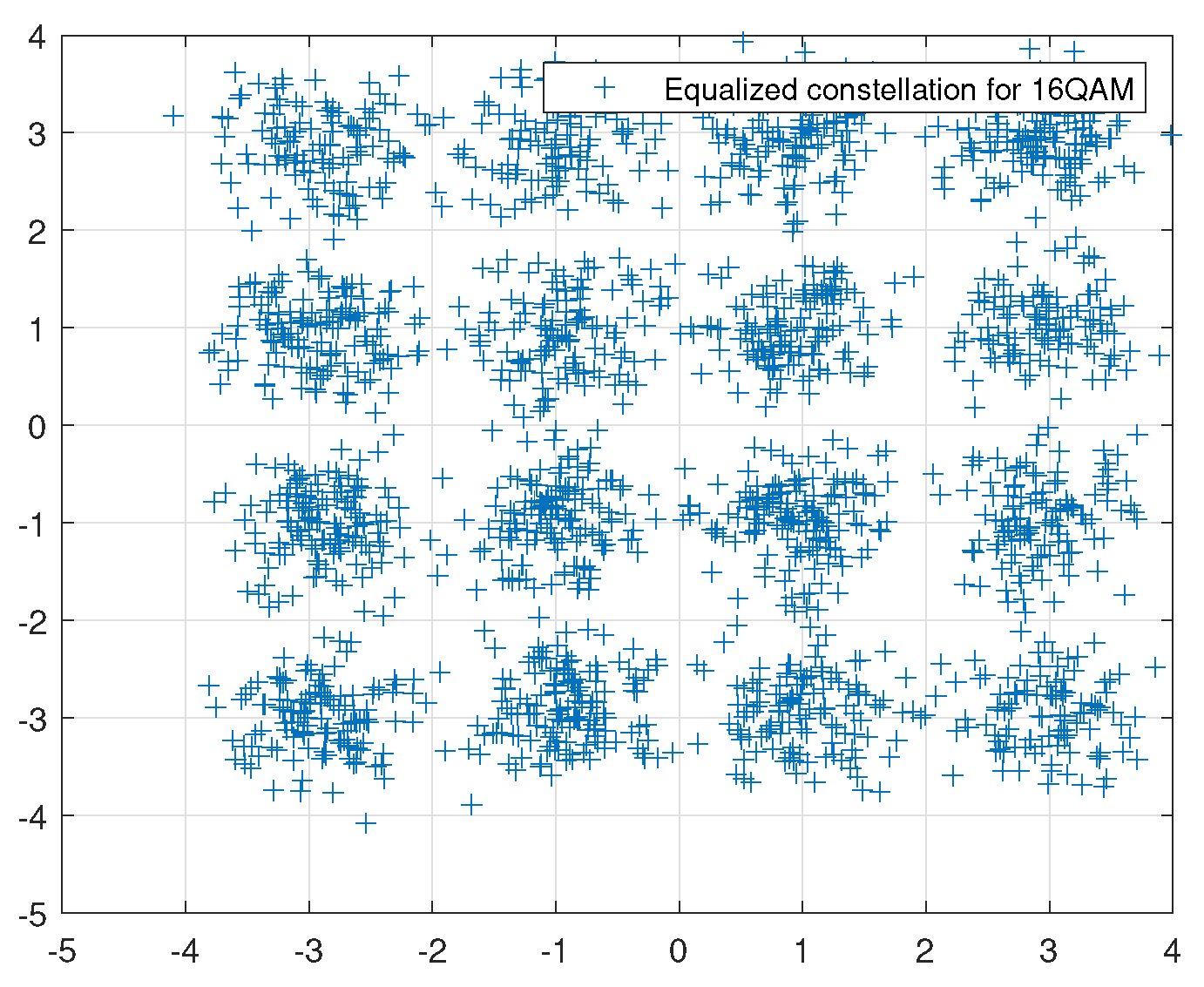
According to [1], when the convolutional noise power $m_p$ is a very small value, the solution for $m_p$ may be given by: $m_p\cong -\frac{C_{1}B}{B_1}$. Obviously, this solution for $m_p$ is less accurate compared to the solution derived from (5). It should be pointed out that the step-size parameter $\mu$ and the equalizer’s tap length N are associated with the function B (6). Thus, if the desired residual ISI is set in (5), we may derive the expected value for B (6) and thus design the system parameters ($\mu$ and N). However, via the function B (6), we have only the outcome of $\mu N$. Thus, if we set a value for the step-size parameter, we also have set automatically a value for the equalizer’s tap length via $\mu N$. Nevertheless, this value N, may not be large enough to compensate for the channel distortions. For example, Figure 2 describes the equalizer’s performance from the residual ISI point of view as a function of the iteration number for Godard’s [2] algorithm, for $\mu =0.00003$ and for $N=13$. Figure 3 describes the equalized constellation output for the 16QAM (Quadrature Amplitude Modulation) input source (a modulation using ± {1,3} levels for in-phase and quadrature components) for $\mu =0.00003$ and $N=13$. According to Figure 2, the residual ISI at the convergence state is approximately $-22$ [dB]. The calculated value for B is $B=0.0039$ where the channel is defined as:

CH1 (initial ISI = 0.88): The channel parameters are determined according to [1]:

$$h\left[n\right]=[0.4851,-0.72765,-0.4851]where\sum _{k=0}^{k=R-1}{\left|h_k\left[n\right]\right|}^2\simeq 1.$$

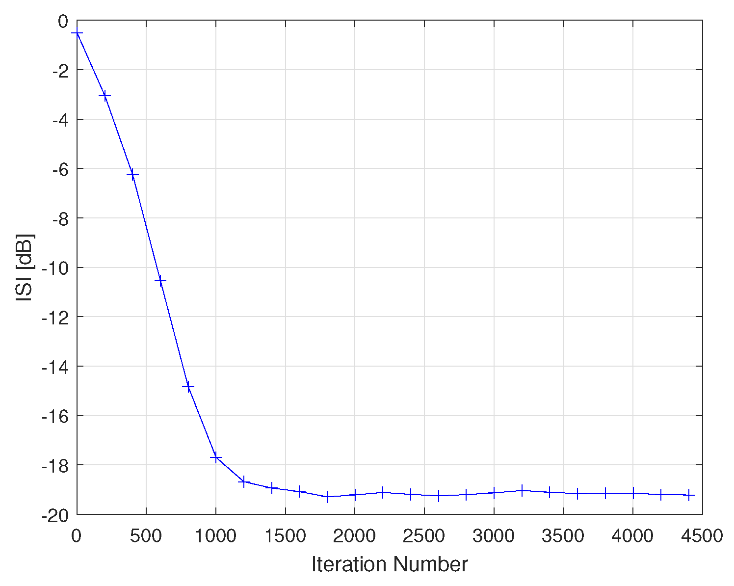
Next, according to (6), $\mu N=B/\left({\sigma }_x^2{\sum }_{k=0}^{k=R-1}{\left|h_k\left[n\right]\right|}^2\right)=0.00039$ since ${\sigma }_x^2=10$ for the 16QAM input sequence. Now, the value of $0.00039$ for $\mu N$ can also be obtained approximately by using $\mu =0.000056$ with $N=7$ or by using $\mu =0.000078$ with $N=5$. Figure 4 and Figure 5 describe the equalizer’s performance from the residual ISI point of view as a function of the iteration number for Godard’s [2] algorithm, for $\mu =0.000056$ with $N=7$ and for $\mu =0.000078$ with $N=5$ respectively. Figure 6 describes the equalized constellation output for the 16QAM input source for $\mu =0.000078$ and $N=5$. Please note that for the three cases: case1 where $\mu =0.00003$ with $N=13$, case2 where $\mu =0.000056$ with $N=7$ and case3 where $\mu =0.000078$ with $N=5$, the value for B is approximately the same. Thus, the equalizer’s performance should have been the same for the three cases. However, this is not what we received. According to Figure 4 and Figure 5, the residual ISI at the convergence state is higher than $-22$ [dB] which implies having some degradation in the equalization performance from the residual ISI point of view. In addition, according to Figure 6, the equalized constellation output is not clear as it is in Figure 3. As a matter of fact, Figure 6 implies that the system suffers from a higher symbol error rate compared to the results from Figure 3. The explanation for not having the same equalization performance for the three cases may be due to the fact that the equalizer’s tap length is not long enough to compensate for the channel distortions. Thus, it is important to have an additional tool that can indicate something on the required equalizer’s tap length that has to be used in the system.

Theorem 1.

The equalizer’s tap length should be set according to:

$$\begin{array}{c}N>>\left|\frac{V_2}{V_1}\right|\\ with\\ V_1=-6a_3{m}_p^2-2a_{12}{m}_p^2-2a_1{m}_p-6{\sigma }_{x_r}^2{a}_3{m}_p-2{\sigma }_{x_i}^2{a}_{12}{m}_p\\ V_2=3{\sigma }_{x_r}^2{a}_3{m}_p-3\frac{E\left[x_r^4\right]}{{\sigma }_{x_r}^2}{a}_3{m}_p\end{array}$$

(10)

Proof of Theorem 1.

The expression for $m_p$ was obtained in [1] via the following expression [1]:

$$\begin{array}{c}E\left[\Delta p_r^2\right]\simeq -2\left(a_{3}3m_p^2+a_{12}{m}_p^2+a_{12}{m}_p{\sigma }_{x_i}^2+3a_{3}E\left[p_r^2{x}_r^2\right]+a_1{m}_p\right)B+B^2\tilde{B}\\ \tilde{B}=15m_p^3{a}_3^2+2a_3{a}_{12}3m_p^3+2a_1{a}_{3}3m_p^2+15a_3^{2}E\left[x_r^2{p}_r^4\right]\\ +2a_3{a}_{12}3m_p^2{\sigma }_{x_i}^2+a_{12}^{2}3m_p^3+2a_1{a}_{12}{m}_p^2\\ +12a_3{a}_{12}E\left[x_r^2{p}_r^2\right]m_p+6a_{12}^2{m}_{p}E\left[x_i^2{p}_i^2\right]+a_1^2{m}_p\\ +12a_1{a}_{3}E\left[x_r^2{p}_r^2\right]+2a_1{a}_{12}{m}_p{\sigma }_{x_i}^2+15a_3^{2}E\left[x_r^4{p}_r^2\right]\\ +12a_3{a}_{12}E\left[x_r^2{p}_r^2\right]{\sigma }_{x_i}^2+a_{12}^2{m}_{p}E\left[x_i^4\right]+a_{12}^{2}3m_p^2{\sigma }_{x_r}^2\\ +2a_1{a}_{12}{m}_p{\sigma }_{x_r}^2+2a_3{a}_{12}{m}_{p}E\left[x_r^4\right]+6a_{12}^{2}E\left[x_i^2{p}_i^2\right]{\sigma }_{x_r}^2\\ +a_1^2{\sigma }_{x_r}^2+2a_1{a}_{3}E\left[x_r^4\right]+2a_1{a}_{12}{\sigma }_{x_i}^2{\sigma }_{x_r}^2+a_3^{2}E\left[x_r^6\right]+2a_3{a}_{12}{\sigma }_{x_i}^{2}E\left[x_r^4\right]+a_{12}^{2}E\left[x_i^4\right]{\sigma }_{x_r}^2\end{array}$$

(11)

where $E\left[\Delta p_r^2\right]=E\left[p_r^2\left[n+1\right]\right]-E\left[p_r^2\left[n\right]\right]$. Please note that $E\left[\Delta p_r^2\right]$ was set to zero in [1] since at the convergence state, the variance of the convolutional noise at time index n and $n+1$ are approximately the same. In addition, the following approximations were done in [1]:

$$\begin{array}{c}E\left[p_r^2{x}_r^2\right]=E\left[p_i^2{x}_i^2\right]\simeq m_p{\sigma }_{x_r}^2\\ E\left[x_r^2{p}_r^4\right]\simeq 3{\sigma }_{x_r}^2{m}_p^2\\ E\left[x_r^4{p}_r^2\right]\simeq E\left[x_r^4\right]m_p\end{array}$$

(12)

Still, according to (2), $x_r$ and $p_r$ are related. Thus, more accurate expressions for (12) can be obtained. In this work, we also use (11) with $E\left[\Delta p_r^2\right]=0$. Unlike the author in [1], we do not use the assumptions of (12). In this work, we derive new expressions for $E\left[p_r^2{x}_r^2\right]$, $E\left[x_r^2{p}_r^4\right]$ and $E\left[x_r^4{p}_r^2\right]$. In order to do this, we need first to see the connection between $m_p$ and $E\left[{\xi }_r^2\left[n\right]\right]$ where ${\xi }_r\left[n\right]$ is the real part of $\xi \left[n\right]$. In the following we denote $\xi \left[n\right]$ as $\xi$. Based on (2), we may write:

$$p_r\left[n\right]=Re\left[{\sum }_k\left(x_r\left[n-k\right]+j{x}_i\left[n-k\right]\right)\left({\xi }_r\left[k\right]+j{\xi }_i\left[k\right]\right)\right]={\sum }_k{x}_r\left[n-k\right]{\xi }_r\left[k\right]-{\sum }_k{x}_i\left[n-k\right]{\xi }_i\left[k\right]$$

(13)

where $\xi \left[n\right]={\xi }_r\left[n\right]+j{\xi }_i\left[n\right]$. By using (13) we may write:

$$\begin{array}{c}E\left[p_r^2\right]=E\left[\left(\sum _{k,r}-\sum _{k,i}\right)\left(\sum _{m,r}-\sum _{m,i}\right)\right]=E\left[\sum _{k,r}\sum _{m,r}+\sum _{k,i}\sum _{m,i}\right]=\\ N{\sigma }_{x_r}^{2}E\left[{\xi }_r^2\right]+N{\sigma }_{x_i}^{2}E\left[{\xi }_i^2\right]=2N{\sigma }_{x_r}^{2}E\left[{\xi }_r^2\right]=m_p\\ \mathrm{where}\\ \sum _{k,r}=\sum _k{x}_r\left[n-k\right]{\xi }_r\left[k\right];\sum _{k,i}=\sum _k{x}_i\left[n-k\right]{\xi }_i\left[k\right]\\ E\left[\sum _{k,r}\sum _{m,r}\right]=\sum _k\sum _m{x}_r\left[n-k\right]x_r\left[n-m\right]{\xi }_r\left[k\right]{\xi }_r\left[m\right]=\sum _k{x}_r^2\left[n-k\right]{\xi }_r^2\left[k\right]=N{\sigma }_{x_r}^{2}E\left[{\xi }_r^2\right]\\ E\left[\sum _{k,i}\sum _{m,i}\right]=\sum _k\sum _m{x}_i\left[n-k\right]x_i\left[n-m\right]{\xi }_i\left[k\right]{\xi }_i\left[m\right]=\sum _k{x}_i^2\left[n-k\right]{\xi }_i^2\left[k\right]=N{\sigma }_{x_i}^{2}E\left[{\xi }_i^2\right]\\ E\left[{\xi }_r^2\right]=E\left[{\xi }_i^2\right]\end{array}$$

(14)

Based on (14) we have:

$$E\left[{\xi }_r^2\right]=\frac{m_p}{2N{\sigma }_{x_r}^2}$$

(15)

Next, we turn to derive the expression for $E\left[x_r^4{p}_r^2\right]$:

$$\begin{array}{c}E\left[x_r^4{p}_r^2\right]=E\left[x_r^4\left(\sum _{k,r}\sum _{m,r}+\sum _{k,i}\sum _{m,i}\right)\right]=E\left[x_r^4\sum _{k,r}\sum _{m,r}\right]+E\left[x_r^4\right]E\left[\sum _{k,i}\sum _{m,i}\right]=\\ \left(N-1\right){\sigma }_{x_r}^{2}E\left[x_r^4\right]E\left[{\xi }_r^2\right]+E\left[x_r^6\right]E\left[{\xi }_r^2\right]+E\left[x_r^4\right]N{\sigma }_{x_i}^{2}E\left[{\xi }_i^2\right]\\ \mathrm{where}\\ E\left[x_r^4\sum _{k,r}\sum _{m,r}\right]=E\left[\sum _k\sum _m{x}_r^4\left[n\right]x_r\left[n-k\right]x_r\left[n-m\right]{\xi }_r\left[k\right]{\xi }_r\left[m\right]\right]=E{\left(\sum _{k=m}\right)}_{k\ne 0}+E\sum _{k=m=0}\\ E{\left(\sum _{k=m}\right)}_{k\ne 0}=\left(N-1\right){\sigma }_{x_r}^{2}E\left[x_r^4\right]E\left[{\xi }_r^2\right]\\ E\sum _{k=m=0}=E\left[x_r^6\right]E\left[{\xi }_r^2\right]\\ E\left[x_r^4\right]E\left[\sum _{k,i}\sum _{m,i}\right]=E\left[x_r^4\right]N{\sigma }_{x_i}^{2}E\left[{\xi }_i^2\right]\end{array}$$

(16)

Based on (15) and (16) we have:

$$E\left[x_r^4{p}_r^2\right]=E\left[x_r^4\right]m_p-E\left[x_r^4\right]\frac{m_p}{2N}+E\left[x_r^6\right]\frac{m_p}{2N{\sigma }_{x_r}^2}$$

(17)

Now, in order to derive the expression for $E\left[x_r^2{p}_r^4\right]$, we need first to get the relationship between $E\left[p_r^4\right]$ and $E\left[{\xi }_r^4\right]$. By using (13) and (15), we may write:

$$\begin{array}{c}E\left[p_r^4\right]=E\left[\sum _{k,r}\sum _{m,r}\sum _{s,r}\sum _{t,r}\right]+E\left[\sum _{k,i}\sum _{m,i}\sum _{s,i}\sum _{t,i}\right]+E\left[\sum _{k,r}\sum _{m,r}\sum _{s,i}\sum _{t,i}\right]+E\left[\sum _{k,i}\sum _{m,i}\sum _{s,r}\sum _{t,r}\right]+\\ E\left[\sum _{k,r}\sum _{s,r}\sum _{m,i}\sum _{t,i}\right]+E\left[\sum _{k,i}\sum _{s,i}\sum _{m,r}\sum _{t,r}\right]+E\left[\sum _{k,r}\sum _{t,r}\sum _{m,i}\sum _{s,i}\right]+E\left[\sum _{k,i}\sum _{t,i}\sum _{m,r}\sum _{s,r}\right]=\\ 2NE\left[{\xi }_r^4\right]E\left[x_r^4\right]+3\left(N-1\right)\frac{m_p^2}{2N}+6\frac{m_p^2}{4}=3m_p^2\\ \mathrm{where}\\ E\left[\sum _{k,i}\sum _{m,i}\sum _{s,i}\sum _{t,i}\right]=E\left[\sum _{k,r}\sum _{m,r}\sum _{s,r}\sum _{t,r}\right]=\\ E\left[\sum _k\sum _m\sum _t\sum _s{x}_r\left[n-k\right]x_r\left[n-m\right]x_r\left[n-t\right]x_r\left[n-s\right]{\xi }_r\left[k\right]{\xi }_r\left[m\right]{\xi }_r\left[t\right]{\xi }_r\left[s\right]\right]=\\ E\sum _{k=m=t=s}+E{\left(\sum _{k=m}\sum _{t=s}\right)}_{k\ne t}+E{\left(\sum _{k=t}\sum _{m=s}\right)}_{k\ne s}+E{\left(\sum _{k=s}\sum _{m=t}\right)}_{k\ne m}=\\ NE\left[{\xi }_r^4\right]E\left[x_r^4\right]+3\left(N-1\right)N{\sigma }_{x_r}^2{\sigma }_{x_r}^{2}E\left[{\xi }_r^2\right]E\left[{\xi }_r^2\right]=\\ NE\left[{\xi }_r^4\right]E\left[x_r^4\right]+3\left(N-1\right)\frac{m_p^2}{4N}\\ \mathrm{and}\\ E\sum _{k=m=t=s}=NE\left[{\xi }_r^4\right]E\left[x_r^4\right]\\ E{\left(\sum _{k=m}\sum _{t=s}\right)}_{k\ne t}=E{\left(\sum _{k=t}\sum _{m=s}\right)}_{k\ne s}=E{\left(\sum _{k=s}\sum _{m=t}\right)}_{k\ne m}=\left(N-1\right)N{\sigma }_{x_r}^2{\sigma }_{x_r}^{2}E\left[{\xi }_r^2\right]E\left[{\xi }_r^2\right]\\ \mathrm{and}\mathrm{where}\\ E\left[\sum _{k,r}\sum _{m,r}\sum _{s,i}\sum _{t,i}\right]=E\left[\sum _{k,r}\sum _{m,r}\right]E\left[\sum _{s,i}\sum _{t,i}\right]=N{\sigma }_{x_r}^{2}E\left[{\xi }_r^2\right]N{\sigma }_{x_i}^{2}E\left[{\xi }_i^2\right]=N{\sigma }_{x_r}^2\frac{m_p}{2N{\sigma }_{x_r}^2}N{\sigma }_{x_i}^2\frac{m_p}{2N{\sigma }_{x_r}^2}=\frac{m_p^2}{4}\\ E\left[\sum _{k,r}\sum _{m,r}\sum _{s,i}\sum _{t,i}\right]=E\left[\sum _{k,i}\sum _{m,i}\sum _{s,r}\sum _{t,r}\right]=E\left[\sum _{k,r}\sum _{s,r}\sum _{m,i}\sum _{t,i}\right]=\\ E\left[\sum _{k,i}\sum _{s,i}\sum _{m,r}\sum _{t,r}\right]=E\left[\sum _{k,r}\sum _{t,r}\sum _{m,i}\sum _{s,i}\right]=E\left[\sum _{k,i}\sum _{t,i}\sum _{m,r}\sum _{s,r}\right]\end{array}$$

(18)

Now by using (17) we may write:

$$E\left[{\xi }_r^4\right]=\frac{3m_p^2}{4N^{2}E\left[x_r^4\right]}$$

(19)

Next we turn to derive the expression for $E\left[x_r^2{p}_r^4\right]$. By using (13), (15) and (19) we have:

$$\begin{array}{c}E\left[x_r^2{p}_r^4\right]=E\left[x_r^2\sum _{k,r}\sum _{m,r}\sum _{s,r}\sum _{t,r}\right]+E\left[x_r^2\sum _{k,i}\sum _{m,i}\sum _{s,i}\sum _{t,i}\right]+E\left[x_r^2\sum _{k,r}\sum _{m,r}\sum _{s,i}\sum _{t,i}\right]+\\ E\left[x_r^2\sum _{k,i}\sum _{m,i}\sum _{s,r}\sum _{t,r}\right]+E\left[x_r^2\sum _{k,r}\sum _{s,r}\sum _{m,i}\sum _{t,i}\right]+E\left[x_r^2\sum _{k,i}\sum _{s,i}\sum _{m,r}\sum _{t,r}\right]+\\ E\left[x_r^2\sum _{k,r}\sum _{t,r}\sum _{m,i}\sum _{s,i}\right]+E\left[x_r^2\sum _{k,i}\sum _{t,i}\sum _{m,r}\sum _{s,r}\right]=\\ E\left[x_r^6\right]\frac{3m_p^2}{4N^{2}E\left[x_r^4\right]}+{\sigma }_{x_r}^{2}3m_p^2+3E\left[x_r^4\right]\frac{m_p^2}{N{\sigma }_{x_r}^2}-3E\left[x_r^4\right]\frac{m_p^2}{2N^2{\sigma }_{x_r}^2}-\frac{3}{N}{\sigma }_{x_r}^2{m}_p^2+\frac{3}{4N^2}{\sigma }_{x_r}^2{m}_p^2\\ \mathrm{where}\\ E\left[x_r^2\sum _{k,r}\sum _{m,r}\sum _{s,r}\sum _{t,r}\right]=E\left[\sum _k\sum _m\sum _t\sum _s{x}_r\left[n-k\right]x_r\left[n-m\right]x_r\left[n-t\right]x_r\left[n-s\right]x_r^2\left[n\right]{\xi }_r\left[k\right]{\xi }_r\left[m\right]{\xi }_r\left[t\right]{\xi }_r\left[s\right]\right]=\\ E\sum _{k=m=t=s}+E{\left(\sum _{k=m}\sum _{t=s}\right)}_{k\ne t}+E{\left(\sum _{k=t}\sum _{m=s}\right)}_{k\ne s}+E{\left(\sum _{k=s}\sum _{m=t}\right)}_{k\ne m}=\\ \left(N-1\right)E\left[x_r^4\right]{\sigma }_{x_r}^{2}E\left[{\xi }_r^4\right]+E\left[x_r^6\right]E\left[{\xi }_r^4\right]+3\left(N-2\right)\left(N-1\right){\sigma }_{x_r}^2{\sigma }_{x_r}^2{\sigma }_{x_r}^{2}E\left[{\xi }_r^2\right]E\left[{\xi }_r^2\right]+\\ \left(3\right)2\left(N-1\right){\sigma }_{x_r}^{2}E\left[x_r^4\right]E\left[{\xi }_r^2\right]E\left[{\xi }_r^2\right]\\ \mathrm{and}\\ E\sum _{k=m=t=s}=\left(N-1\right)E\left[x_r^4\right]{\sigma }_{x_r}^{2}E\left[{\xi }_r^4\right]+E\left[x_r^6\right]E\left[{\xi }_r^4\right]\\ E{\left(\sum _{k=m}\sum _{t=s}\right)}_{k\ne t}=\left(N-2\right)\left(N-1\right){\sigma }_{x_r}^2{\sigma }_{x_r}^2{\sigma }_{x_r}^{2}E\left[{\xi }_r^2\right]E\left[{\xi }_r^2\right]+2\left(N-1\right){\sigma }_{x_r}^{2}E\left[x_r^4\right]E\left[{\xi }_r^2\right]E\left[{\xi }_r^2\right]\\ E{\left(\sum _{k=m}\sum _{t=s}\right)}_{k\ne t}=E{\left(\sum _{k=t}\sum _{m=s}\right)}_{k\ne s}=E{\left(\sum _{k=s}\sum _{m=t}\right)}_{k\ne m}\\ \mathrm{and}\mathrm{where}\\ E\left[x_r^2\sum _{k,i}\sum _{m,i}\sum _{s,i}\sum _{t,i}\right]=E\left[x_r^2\right]E\left[\sum _{k,i}\sum _{m,i}\sum _{s,i}\sum _{t,i}\right]=E\left[x_r^2\right]\left(NE\left[{\xi }_i^4\right]E\left[x_i^4\right]+3\left(N-1\right)\frac{m_p^2}{4N}\right)=\\ E\left[x_r^2\right]\left(N\frac{3m_p^2}{4N^{2}E\left[x_r^4\right]}E\left[x_i^4\right]+3\left(N-1\right)\frac{m_p^2}{4N}\right)=E\left[x_r^2\right]\left(\frac{3m_p^2}{4N}+3\left(N-1\right)\frac{m_p^2}{4N}\right)={\sigma }_{x_r}^2\frac{3m_p^2}{4}\\ E\left[x_r^2\sum _{k,r}\sum _{m,r}\sum _{s,i}\sum _{t,i}\right]=E\left[x_r^2\sum _{k,r}\sum _{m,r}\right]E\left[\sum _{s,i}\sum _{t,i}\right]=\\ N{\sigma }_{x_i}^{2}E\left[{\xi }_i^2\right]\left(\left(N-1\right){\sigma }_{x_r}^2{\sigma }_{x_r}^{2}E\left[{\xi }_r^2\right]+E\left[x_r^4\right]E\left[{\xi }_r^2\right]\right)=\\ N{\sigma }_{x_i}^2\frac{m_p}{2N{\sigma }_{x_r}^2}\left(\left(N-1\right){\sigma }_{x_r}^2{\sigma }_{x_r}^2\frac{m_p}{2N{\sigma }_{x_r}^2}+E\left[x_r^4\right]\frac{m_p}{2N{\sigma }_{x_r}^2}\right)=\frac{m_p}{2}\left(\left(N-1\right){\sigma }_{x_r}^2\frac{m_p}{2N}+E\left[x_r^4\right]\frac{m_p}{2N{\sigma }_{x_r}^2}\right)\\ \mathrm{where}\\ E\left[x_r^2\sum _{k,r}\sum _{m,r}\right]=E\left[\sum _k\sum _m{x}_r^2\left[n\right]x_r\left[n-k\right]x_r\left[n-m\right]{\xi }_r\left[k\right]{\xi }_r\left[m\right]\right]=E{\left(\sum _{k=m}\right)}_{k\ne 0}+E\sum _{k=m=0}\\ E{\left(\sum _{k=m}\right)}_{k\ne 0}=\left(N-1\right){\sigma }_{x_r}^2{\sigma }_{x_r}^{2}E\left[{\xi }_r^2\right];E\sum _{k=m=0}=E\left[x_r^4\right]E\left[{\xi }_r^2\right];E\left[\sum _{s,i}\sum _{t,i}\right]=N{\sigma }_{x_i}^{2}E\left[{\xi }_i^2\right]\\ \mathrm{and}\\ E\left[x_r^2\sum _{k,r}\sum _{m,r}\sum _{s,i}\sum _{t,i}\right]=E\left[x_r^2\sum _{k,i}\sum _{m,i}\sum _{s,r}\sum _{t,r}\right]=E\left[x_r^2\sum _{k,r}\sum _{s,r}\sum _{m,i}\sum _{t,i}\right]=\\ E\left[x_r^2\sum _{k,i}\sum _{s,i}\sum _{m,r}\sum _{t,r}\right]=E\left[x_r^2\sum _{k,r}\sum _{t,r}\sum _{m,i}\sum _{s,i}\right]=E\left[x_r^2\sum _{k,i}\sum _{t,i}\sum _{m,r}\sum _{s,r}\right]\end{array}$$

(20)

Next we turn to derive the expression for $E\left[x_r^2{p}_r^2\right]$. By using (13)–(15) we may write:

$$\begin{array}{c}E\left[x_r^2{p}_r^2\right]=E\left[x_r^2\sum _{k,r}\sum _{m,r}\right]+E\left[x_r^2\right]E\left[\sum _{k,i}\sum _{m,i}\right]=\\ \\ {\sigma }_{x_r}^2{m}_p-{\sigma }_{x_r}^2\frac{m_p}{2N}+E\left[x_r^4\right]\frac{m_p}{2N{\sigma }_{x_r}^2}\\ \mathrm{where}\\ E\left[x_r^2\right]E\left[\sum _{k,i}\sum _{m,i}\right]={\sigma }_{x_r}^{2}N{\sigma }_{x_i}^{2}E\left[{\xi }_i^2\right]={\sigma }_{x_r}^{2}N{\sigma }_{x_i}^2\frac{m_p}{2N{\sigma }_{x_r}^2}={\sigma }_{x_i}^2\frac{m_p}{2}\\ E\left[x_r^2\sum _{k,r}\sum _{m,r}\right]=E\left[\sum _k\sum _m{x}_r^2\left[n\right]x_r\left[n-k\right]x_r\left[n-m\right]{\xi }_r\left[k\right]{\xi }_r\left[m\right]\right]=E{\left(\sum _{k=m}\right)}_{k\ne 0}+E\sum _{k=m=0}=\\ \left(N-1\right){\sigma }_{x_r}^2{\sigma }_{x_r}^{2}E\left[{\xi }_r^2\right]+E\left[x_r^4\right]E\left[{\xi }_r^2\right]=\left(N-1\right){\sigma }_{x_r}^2\frac{m_p}{2N}+E\left[x_r^4\right]\frac{m_p}{2N{\sigma }_{x_r}^2}\\ \mathrm{and}\\ E{\left(\sum _{k=m}\right)}_{k\ne 0}=\left(N-1\right){\sigma }_{x_r}^2{\sigma }_{x_r}^{2}E\left[{\xi }_r^2\right];E\sum _{k=m=0}=E\left[x_r^4\right]E\left[{\xi }_r^2\right]\end{array}$$

(21)

Now we substitute the expressions for $E\left[p_r^2{x}_r^2\right]$ (21), $E\left[x_r^2{p}_r^4\right]$ (20), $E\left[x_r^4{p}_r^2\right]$ (17) and $E\left[p_i^2{x}_i^2\right]$ ($E\left[p_i^2{x}_i^2\right]=E\left[p_r^2{x}_r^2\right]$) into (11) and obtain:

$$\begin{array}{c}E\left[\Delta p_r^2\right]\simeq Vb+b^{2}S\\ \mathrm{where}\\ V=V_{1}N+V_2\\ V_1=-6a_3{m}_p^2-2a_{12}{m}_p^2-2a_1{m}_p-6{\sigma }_{x_r}^2{a}_3{m}_p-2{\sigma }_{x_i}^2{a}_{12}{m}_p\\ V_2=3{\sigma }_{x_r}^2{a}_3{m}_p-3\frac{E\left[x_r^4\right]}{{\sigma }_{x_r}^2}{a}_3{m}_p\\ S=A_1{N}^2+A_{2}N+A_3\\ A_1=2{\sigma }_{x_i}^2{\sigma }_{x_r}^2{a}_1{a}_{12}+12{\sigma }_{x_i}^2{\sigma }_{x_r}^2{a}_3{a}_{12}{m}_p+2{\sigma }_{x_i}^2{a}_1{a}_{12}{m}_p+6{\sigma }_{x_i}^2{a}_3{a}_{12}{m}_p^2+\\ 2E\left[x_r^4\right]{\sigma }_{x_i}^2{a}_3{a}_{12}+6{\sigma }_{x_r}^4{a}_{12}^2{m}_p+{\sigma }_{x_r}^2{a}_1^2+12{\sigma }_{x_r}^2{a}_1{a}_3{m}_p+2{\sigma }_{x_r}^2{a}_1{a}_{12}{m}_p+\\ 45{\sigma }_{x_r}^2{a}_3^2{m}_p^2+12{\sigma }_{x_r}^2{a}_3{a}_{12}{m}_p^2+9{\sigma }_{x_r}^2{a}_{12}^2{m}_p^2+E\left[x_r^4\right]{\sigma }_{x_r}^2{a}_{12}^2+a_1^2{m}_p+\\ 6a_1{a}_3{m}_p^2+2E\left[x_r^4\right]a_1{a}_3+2a_1{a}_{12}{m}_p^2+15a_3^2{m}_p^3+15E\left[x_r^4\right]a_3^2{m}_p+\\ E\left[x_r^6\right]a_3^2+6a_3{a}_{12}{m}_p^3+2E\left[x_r^4\right]a_3{a}_{12}{m}_p+3a_{12}^2{m}_p^3+E\left[x_r^4\right]a_{12}^2{m}_p\\ A_2=3E\left[x_r^4\right]a_{12}^2{m}_p-\frac{15}{2}E\left[x_r^4\right]a_3^2{m}_p-45{\sigma }_{x_r}^2{a}_3^2{m}_p^2-3{\sigma }_{x_r}^2{a}_{12}^2{m}_p^2-\\ 3{\sigma }_{x_r}^4{a}_{12}^2{m}_p-6{\sigma }_{x_r}^2{a}_3{a}_{12}{m}_p^2+45\frac{E\left[x_r^4\right]}{{\sigma }_{x_r}^2}{a}_3^2{m}_p^2+3\frac{E\left[x_r^4\right]}{{\sigma }_{x_r}^2}{a}_{12}^2{m}_p^2-\\ 6{\sigma }_{x_r}^2{a}_1{a}_3{m}_p+\frac{15}{2}\frac{E\left[x_r^6\right]}{{\sigma }_{x_r}^2}{a}_3^2{m}_p+6\frac{E\left[x_r^4\right]}{{\sigma }_{x_r}^2}{a}_3{a}_{12}{m}_p^2-\\ 6{\sigma }_{x_i}^2{\sigma }_{x_r}^2{a}_3{a}_{12}{m}_p+6\frac{E\left[x_r^4\right]}{{\sigma }_{x_r}^2}{a}_1{a}_3{m}_p+6E\left[x_r^4\right]\frac{{\sigma }_{x_i}^2}{{\sigma }_{x_r}^2}{a}_3{a}_{12}{m}_p\\ A_3=\frac{45}{4}{\sigma }_{x_r}^2{a}_3^2{m}_p^2-\frac{45}{2}\frac{E\left[x_r^4\right]}{{\sigma }_{x_r}^2}{a}_3^2{m}_p^2+\frac{45}{4}\frac{E\left[x_r^6\right]}{E\left[x_r^4\right]}{a}_3^2{m}_p^2\\ b=\mu {\sigma }_x^2\sum _{k=0}^{k=R-1}{\left|h_k\left[n\right]\right|}^2\end{array}$$

(22)

Next we set $E\left[\Delta p_r^2\right]=0$ and with the help of (22) we obtain for $b\ne 0$:

$$b=-\frac{V}{S}=-\frac{V_{1}N+V_2}{A_1{N}^2+A_{2}N+A_3}$$

(23)

Now, according to B (6), we have a linear relation between the step-size parameter $\mu$ and the equalizer’s tap length N which was obtained in [1] under the assumption that the equalizer reaches a relative low residual ISI with the selected equalizer’s tap length N. Therefore, if we have that:

$$\begin{array}{c}\left|A_1\right|>\left|A_2\right|;\left|A_1\right|>\left|A_3\right|\\ \left|V_{1}N\right|>>\left|V_2\right|\Rightarrow N>>\left|\frac{V_2}{V_1}\right|\end{array}$$

(24)

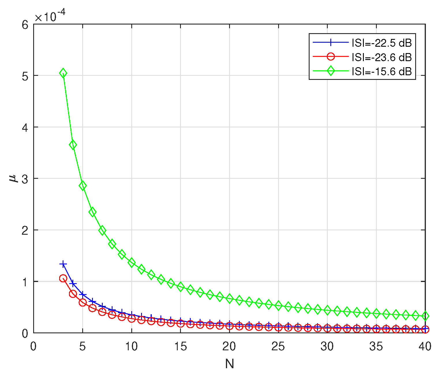
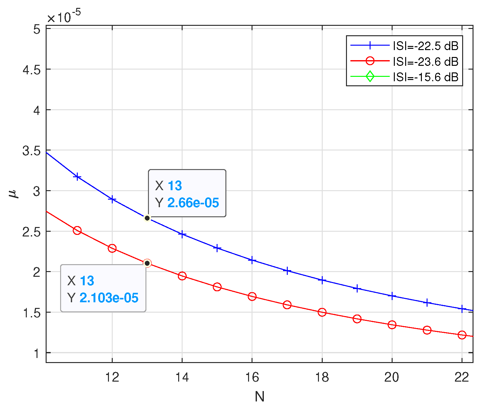
We obtain a linear relation between the step-size parameter $\mu$ and the equalizer’s tap length N and obtain a condition on the parameter N. Please note that for $m_p\to 0$, the inequalities $\left|A_1\right|>\left|A_2\right|$ and $\left|A_1\right|>\left|A_3\right|$ are always true. Figure 7 describes the step-size parameter $\mu$ calculated via (23) for the 16QAM input case, valid for CH1 and for Godard’s algorithm, as a function of the equalizer’s tap length N for three levels of residual ISI. It should be pointed out that when the equalizer leaves the system with a residual ISI of $-15.6$ dB, the system will suffer from a relative high symbol error rate compared to the case where the residual ISI is $-23.6$ dB or $-22.5$ dB. According to Figure 7, there is a range of values for N, where the relation between the step-size parameter $\mu$ and the equalizer’s tap length N is approximately linear.

Now, let us examine the expression of $\left|\frac{V_2}{V_1}\right|$ (24) for three cases of residual ISI (three cases of $m_p$), for the 16QAM input case, CH1 and for Godard’s algorithm:

case1: $\mathrm{ISI}=-22.5$ dB ($m_p=0.027992$):

$$N>>\left|\frac{V_2}{V_1}\right|=0.69445\to 20\left|\frac{V_2}{V_1}\right|\simeq 14$$

case2: $\mathrm{ISI}=-23.6$ dB ($m_p=0.0218233$):

$$N>>\left|\frac{V_2}{V_1}\right|=0.69694\to 20\left|\frac{V_2}{V_1}\right|\simeq 14$$

case3: $\mathrm{ISI}=-15.6$ dB ($m_p=0.1378045$):

$$N>>\left|\frac{V_2}{V_1}\right|=0.65295\to 20\left|\frac{V_2}{V_1}\right|\simeq 13$$

According to Figure 7, a tap length of $N=13$ or $N=14$ is lying approximately on the linear curve of the step-size parameter $\mu$ as a function of the equalizer’s tap length N. □

3. Discussion

In the previous section we have shown that by multiplying the expression of $\left|\frac{V_2}{V_1}\right|$ by twenty gives a value for N that is lying approximately on the linear curve of $\mu$ as a function of N. Now, let us choose $N=13$ for the three cases of the desired residual ISI from the previous section ($ISI=-22.5$ dB, $ISI=-23.6$ dB, $ISI=-15.6$ dB) and calculate the step-size parameter $\mu$ via (4)–(6) for the 16QAM input case, CH1 and Godard’s [2] algorithm. According to (4)–(6):

• case1: $\mathrm{ISI}=-22.5$ dB ($m_p=0.027992$): $B=3.2913\times {10}^{-3}\to \mu =2.5318\times {10}^{-5}$
• case2: $\mathrm{ISI}=-23.6$ dB ($m_p=0.0218233$): $B=2.6003\times {10}^{-3}\to \mu =2.0002\times {10}^{-5}$
• case3: $\mathrm{ISI}=-15.6$ dB ($m_p=0.1378045$): $B=1.3002\times {10}^{-2}\to \mu =1.0002\times {10}^{-4}$

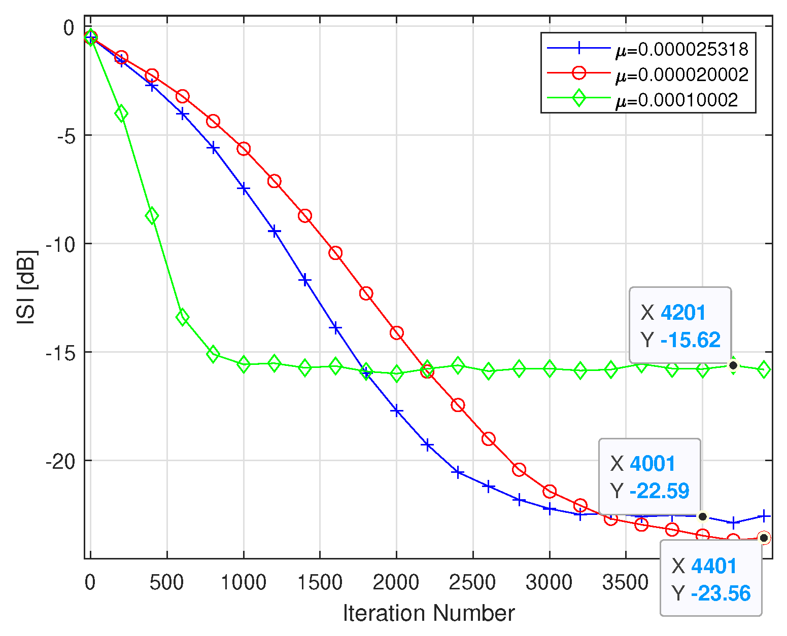
Next, we will show that the obtained values for $\mu$ via (4)–(6) for $N=13$ really achieve the desired residual ISI. Figure 8 shows the simulated equalization performance from the residual ISI point of view for the 16QAM input case, CH1, $N=13$ and for Godard’s [2] algorithm. According to Figure 8, the obtained values for $\mu$ via (4)–(6) really achieve the desired residual ISI for $N=13$.

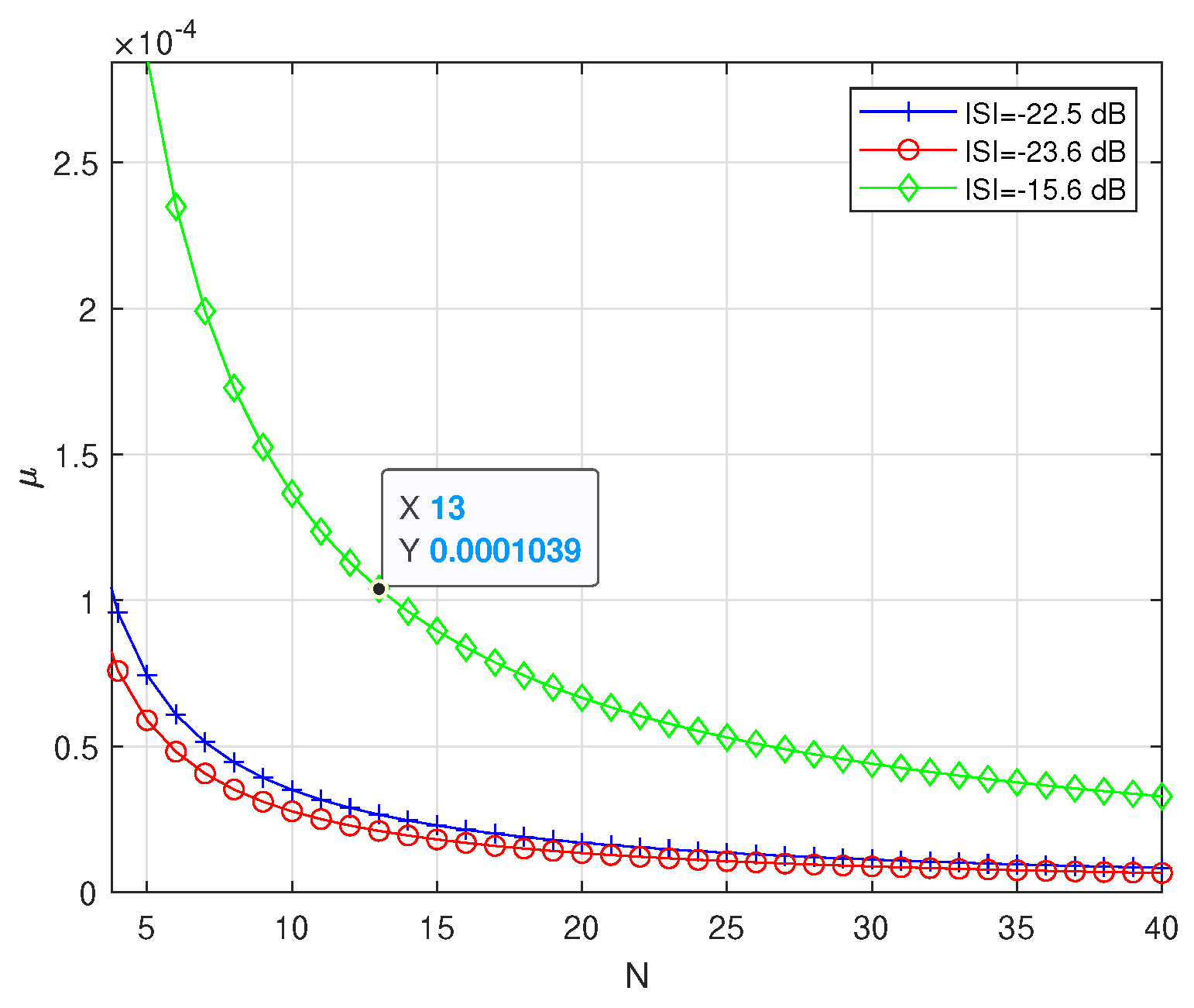
Now, let us compare the values for the step-size parameter $\mu$ obtained via (4)–(6) with those obtained via Figure 7 for $N=13$. Figure 9 and Figure 10 are zoomed in versions of Figure 7.

According to Figure 9 and Figure 10, there is a high correlation between the obtained values for $\mu$ via (4)–(6) with those obtained from Figure 9 and Figure 10 for $N=13$. Thus, multiplying the expression of $\left|\frac{V_2}{V_1}\right|$ (24) by twenty gives a good working value for N for CH1. However, since CH1 is considered as an easy channel, the expression of $\left|\frac{V_2}{V_1}\right|$ (24) should be multiplied by a factor greater than twenty (maybe thirty or more) for harder channels.

Please note that for small values for $m_p$, the expression of $\left|\frac{V_2}{V_1}\right|$ is approximately independent with $m_p$. The equalizer’s tap length should be set large enough such that it can compensate for the channel distortions regardless of the desired residual ISI. Thus, the equalizer’s tap length N should be derived for the low valued $m_p$ case.

References

- Pinchas, M. A Closed Approximated Formed Expression for the Achievable Residual Intersymbol Interference Obtained by Blind Equalizers. Signal Process. 2010, 90, 1940–1962. [Google Scholar] [CrossRef]
- Godard, D.N. Self recovering equalization and carrier tracking in two-dimenional data communication system. IEEE Trans. Commun. 1980, 28, 1867–1875. [Google Scholar] [CrossRef]
- Nikias, C.L.; Petropulu, A.P. (Eds.) Higher-Order Spectra Analysis a Nonlinear Signal Processing Framework; Prentice-Hall: Enlewood Cliffs, NJ, USA, 1993; Chapter 9; pp. 419–425. [Google Scholar]
- Haykin, S. Adaptive Filter Theory. In Blind deconvolution; Haykin, S., Ed.; Prentice-Hall: Englewood Cliffs, NJ, USA, 1991; Chapter 20. [Google Scholar]
- Pinchas, M. A novel expression for the achievable MSE performance obtained by blind adaptive equalizers. Signal Image Video Process. 2013, 7, 67–74. [Google Scholar] [CrossRef]
- Shalvi, O.; Weinstein, E. New criteria for blind deconvolution of nonminimum phase systems (channels). IEEE Trans. Inf. Theory 1990, 36, 312–321. [Google Scholar] [CrossRef]
- Gul, M.M.U.; Sheikh, S.A. Design and implementation of a blind adaptive equalizer using Frequency Domain Square Contour Algorithm. Digit. Signal. Process. 2010, 20, 1697–1710. [Google Scholar]
- Sheikh, S.A.; Fan, P. New Blind Equalization techniques based on improved square contour algorithm. Digit. Signal. Process. 2008, 18, 680–693. [Google Scholar] [CrossRef]
- Thaiupathump, T.; He, L.; Kassam, S.A. Square contour algorithm for blind equalization of QAM signals. Signal Process. 2006, 86, 3357–3370. [Google Scholar] [CrossRef]
- Sharma, V.; Raj, V.N. Convergence and performance analysis of Godard family and multimodulus algorithms for blind equalization. IEEE Trans. Signal Process. 2005, 53, 1520–1533. [Google Scholar] [CrossRef]
- Yuan, J.T.; Lin, T.C. Equalization and Carrier Phase Recovery of CMA and MMA in BlindAdaptive Receivers. IEEE Trans. Signal Process. 2010, 58, 3206–3217. [Google Scholar] [CrossRef]
- Yuan, J.T.; Tsai, K.D. Analysis of the multimodulus blind equalization algorithm in QAM communication systems. IEEE Trans. Commun. 2005, 53, 1427–1431. [Google Scholar] [CrossRef]
- Wu, H.C.; Wu, Y.; Principe, J.C.; Wang, X. Robust switching blind equalizer for wireless cognitive receivers. IEEE Trans. Wirel. Commun. 2008, 7, 1461–1465. [Google Scholar]
- Pinchas, M.; Bobrovsky, B.Z. A Maximum Entropy approach for blind deconvolution. Signal Process. 2006, 86, 2913–2931. [Google Scholar] [CrossRef]
- Abrar, S.; Nandi, A.S. Blind Equalization of Square-QAM Signals: A Multimodulus Approach. IEEE Trans. Commun. 2010, 58, 1674–1685. [Google Scholar] [CrossRef]
- Vanka, R.N.; Murty, S.B.; Mouli, B.C. Performance comparison of supervised and unsupervised/blind equalization algorithms for QAM transmitted constellations. In Proceedings of the 2014 International Conference on Signal Processing and Integrated Networks (SPIN), Noida, India, 20–21 February 2014; pp. 316–321. [Google Scholar]
- Ram Babu, T.; Kumar, P.R. Blind Channel Equalization Using CMA Algorithm. In Proceedings of the 2009 International Conference on Advances in Recent Technologies in Communication and Computing, Kottayam, Kerala, India, 27–28 October 2009; pp. 680–683. [Google Scholar]
- Qin, Q.; Huahua, L.; Tingyao, J. A new study on VCMA-based blind equalization for underwater acoustic communications. In Proceedings of the Proceedings 2013 International Conference on Mechatronic Sciences, Electric Engineering and Computer (MEC), Shengyang, China, 20–22 December 2013; pp. 3526–3529. [Google Scholar]
- Miranda, M.D.; Silva, M.T.M.; Nascimento, V.H. Avoiding Divergence in the Shalvi Weinstein Algorithm. IEEE Trans. Signal Process. 2008, 56, 5403–5413. [Google Scholar] [CrossRef]
- Pinchas, M. Symbol Error Rate as a Function of the Residual ISI Obtained by Blind Adaptive Equalizers for the SIMO and Fractional Gaussian Noise Case. Math. Probl. Eng. 2013, 2013, 860389. [Google Scholar] [CrossRef]
- Pinchas, M. Residual ISI Obtained by Blind Adaptive Equalizers and Fractional Noise. Math. Probl. Eng. 2013, 2013, 972174. [Google Scholar] [CrossRef]
- Goldberg, H.; Pinchas, M. A Novel Technique for Achieving the Approximated ISI at the Receiver for a 16QAM Signal sent via a FIR Channel based only on the Received Information and Statistical Techniques. Entropy 2020, 22, 708. [Google Scholar] [CrossRef] [PubMed]
- Nandi, A.K. (Ed.) Blind Estimation Using Higher-Order Statistics; Kluwer Academic: Boston, MA, USA, 1999; Chapter 2. [Google Scholar]
Figure 1.
Block diagram of the system.
Figure 2.
Equalizer’s performance from the residual inter-symbol-interference (ISI) point of view for and .
Figure 3.
Equalized Constellation output for and .
Figure 4.
Equalizer’s performance from the residual ISI point of view for and .
Figure 5.
Figure 6.
Figure 7.
The step-size parameter calculated via (23) for the 16QAM input case, valid for CH1 and for Godard’s algorithm, as a function of the equalizer’s tap length for three levels of residual ISI.
Figure 8.
Equalizer’s performance from the residual ISI point of view for .
Figure 9.
Figure 10.
Publisher’s Note: MDPI stays neutral with regard to jurisdictional claims in published maps and institutional affiliations. |
© 2020 by the author. Licensee MDPI, Basel, Switzerland. This article is an open access article distributed under the terms and conditions of the Creative Commons Attribution (CC BY) license (https://creativecommons.org/licenses/by/4.0/).
Share and Cite
MDPI and ACS Style
Pinchas, M. The Tap-Length Associated with the Blind Adaptive Equalization/Deconvolution Problem . Eng. Proc. 2020, 3, 2. https://0-doi-org.brum.beds.ac.uk/10.3390/IEC2020-06968
AMA Style
Pinchas M. The Tap-Length Associated with the Blind Adaptive Equalization/Deconvolution Problem . Engineering Proceedings. 2020; 3(1):2. https://0-doi-org.brum.beds.ac.uk/10.3390/IEC2020-06968
Chicago/Turabian StylePinchas, Monika. 2020. "The Tap-Length Associated with the Blind Adaptive Equalization/Deconvolution Problem " Engineering Proceedings 3, no. 1: 2. https://0-doi-org.brum.beds.ac.uk/10.3390/IEC2020-06968