Drinking Water Tank Level Analysis with ARIMA Models: A Case Study †


1
Department of Civil Engineering, University of Salerno, 84084 Fisciano, Italy
2
Department of Information and Electrical Engineering and Applied Mathematics, University of Salerno, 84084 Fisciano, Italy
*
Author to whom correspondence should be addressed.
†
Presented at the 4th EWaS International Conference: Valuing the Water, Carbon, Ecological Footprints of Human Activities, Online, 24–27 June 2020.
Environ. Sci. Proc. 2020, 2(1), 33; https://0-doi-org.brum.beds.ac.uk/10.3390/environsciproc2020002033
Published: 22 August 2020
(This article belongs to the Proceedings of The 4th EWaS International Conference: Valuing the Water, Carbon, Ecological Footprints of Human Activities)
Abstract
:The operational management of tanks for urban water distribution networks is usually a critical element due to the dynamic nature of the water demand and the age of the distribution networks themselves. Today, in a context of water resource scarcity, optimal management is a key point for the sustainable management of urban systems. For this purpose, it is useful to implement predictive tools, able to provide short-term forecasts to inform urban water managers on the most suitable procedure to be applied in the case of routine or critical events. A possible approach is to use autoregressive integrated moving average (ARIMA) models, which combine the autoregression and the moving average approaches, with the possibility to work on a differenced series of the data. They can further embed a seasonal- component (Seasonal ARIMA models), to account for possible periodic patterns in the observed data. In this study, the data of water levels measured from May 2018 to 10 January 2019 in a water storage tank in the area of Benevento, Campania region (Italy), were considered as a case study. The standard ARIMA techniques were applied to find the best model for this dataset, according to “Deviance Information Criterion” (DIC) and “Bayesian Information Criterion” (BIC) optimization. The results are discussed, shedding light on the behaviour of the time series with reference to the management of the infrastructure and the dataset. The residual analysis, carried out to check if the autocorrelation was still present and if the residuals were normally distributed, revealed a narrow distribution. Small values were found throughout the dataset, except for a few periods, corresponding to the imputed data. This application represents a preliminary step of more detailed research that will be carried out to detect the best model for forecasting tank levels for the case study to help to manage the urban water supply.
1. Introduction
The management of water distribution networks (WDNs) relies on water utility operations consisting of usually quick responses to either water demand or source variations as well as the effects of network aging [1,2]. Recently, the development of real-time control (RTC) strategies based on the use of measurement devices, with compact technology at affordable prices, has been facilitated by their straightforward implementation in Internet of Things (IoT) technologies as well as in Supervisory Control and Data Acquisition (SCADA) systems [3]. IoT allows automatic WDN monitoring and control as well as SMS alerting by operating on object components, interconnected through low-cost wired and wireless network sensors [4,5]. SCADA systems consist of distributed control systems that allow devices to be turned on or off remotely while displaying real-time operations in a graphical user interface (GUI) for high-level process supervisory management [6,7].
In this evolving context, storage tanks play a key role, actually acting as lungs [8]—that is, by balancing instantaneous flow variations in the water demand pattern as well as compensating abrupt interruptions of the water feed to the storage tank, as in cases of drought periods or electricity shortages in pumping stations delivering water, when the tank level fluctuates within a fixed range of levels. Water tank levels can be modelled through hydraulic models when the water demand and the management rules and operations are known, but in practical applications, the latter facts are not always fully known. Water demand/tank level prediction and forecasting are therefore a crucial step for supporting decision making regarding operating actions.
From a “modellistic” point of view, the AutoRegressive Integrated Moving Average (ARIMA) typology of models is well established, having been applied in the field of water demand forecasting for a long time [8,9,10,11]. This is justified by the fact that the model follows the trend at different time scales. Despite the applications in urban water demand, there is a gap in the literature concerning the use of ARIMA models for tank water levels [12]. In [13], the link between the water supply, consumer demand and water level at the tank is, however, discussed, with the aim of providing a practical tool for water utilities to take prompt action based on water level variations [14]. The definition of ARIMA models or, more generally, time-series analysis techniques applied to water levels would allow the definition of water leakages at the tank as well, helping to save water, on one hand, and treatment costs related to chlorination or purifying techniques. This is an aspect of paramount importance as the circumstance in which the tank is not able to serve due to water scarcity is not rare, whereas there is a waste of the resource when the water inflow is not controlled [14].
2. Methodology
In this paper, we assess the performance of one of the most conventional linear models, widely used in the literature for the forecasting and management of several datasets: the Box–Jenkins/ARIMA model (see, for instance, [13,15,16,17,18]).
The order of an ARIMA model is represented by the notation ARIMA (p, d, q), where p, d and q are, respectively, the order of the autoregressive part, the order of the differencing and the order of the moving-average process. The general source formula is:
in which Yt is the value of the series observed at the time t, B is the delay operator, and are the autoregressive and the moving average polynomials and et is the difference between the observed value Yt and the forecast at the time t. In the case study presented in this paper, the chosen model is ARIMA (2, 1, 2), according to “Deviance Information Criterion” (DIC) and “Bayesian Information Criterion” (BIC) optimization. The choice was performed with the aid of the statistical program “R”.
3. Dataset Analysis
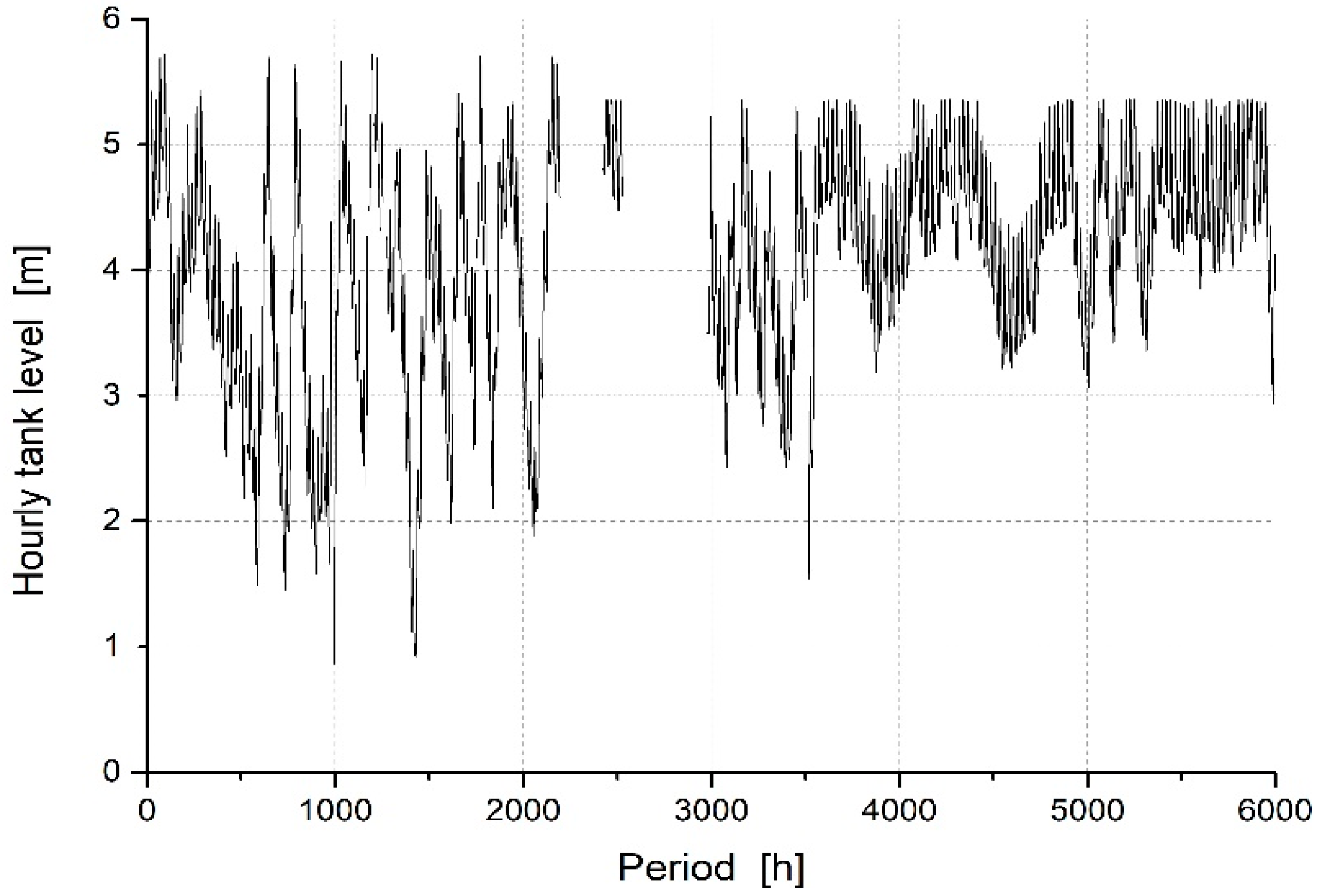
This statistical study was performed on the time series of the levels observed at the Gesuiti water tank, located in the neighbourhood of Pezzapiana, of the water supply system of the town of Benevento, Italy. The data were measured almost continuously and with a time interval never smaller than 5 min (minimum of 12 samples per hour), from 10:00 of 5 May 2018 to 9:00 of 10 January 2019. Hourly averages were calculated with the available data, resulting in a number of 6000 periods in total. A plot of the input dataset is shown in Figure 1. It can be noticed that the maximum levels observed are never larger than zmax = 5.72 m. This is basically due to the presence of an automatic system of water outlet—that is, a tank spillway—which is allocated at an elevation of 5.80 m, consistent with the observed value of zmax.
Two large intervals of data were missing, from 19:00 of 4 August 2018 to 9:00 of 14 August 2018, and from 16:00 of 18 August 2018 to 13:00 of 6 September 2018. Since the dataset needs to be continuous for the Time Series Analysis (TSA) techniques, a preliminary Deterministic Decomposition model (DD-TSA) [15] was calibrated on the first 2193 data, in order to impute the missing data.
When the number of missing measurements was smaller than 10, the missing data were imputed simply with the last available data. On the contrary, for the two large intervals described above, the results of the DD-TSA were used.
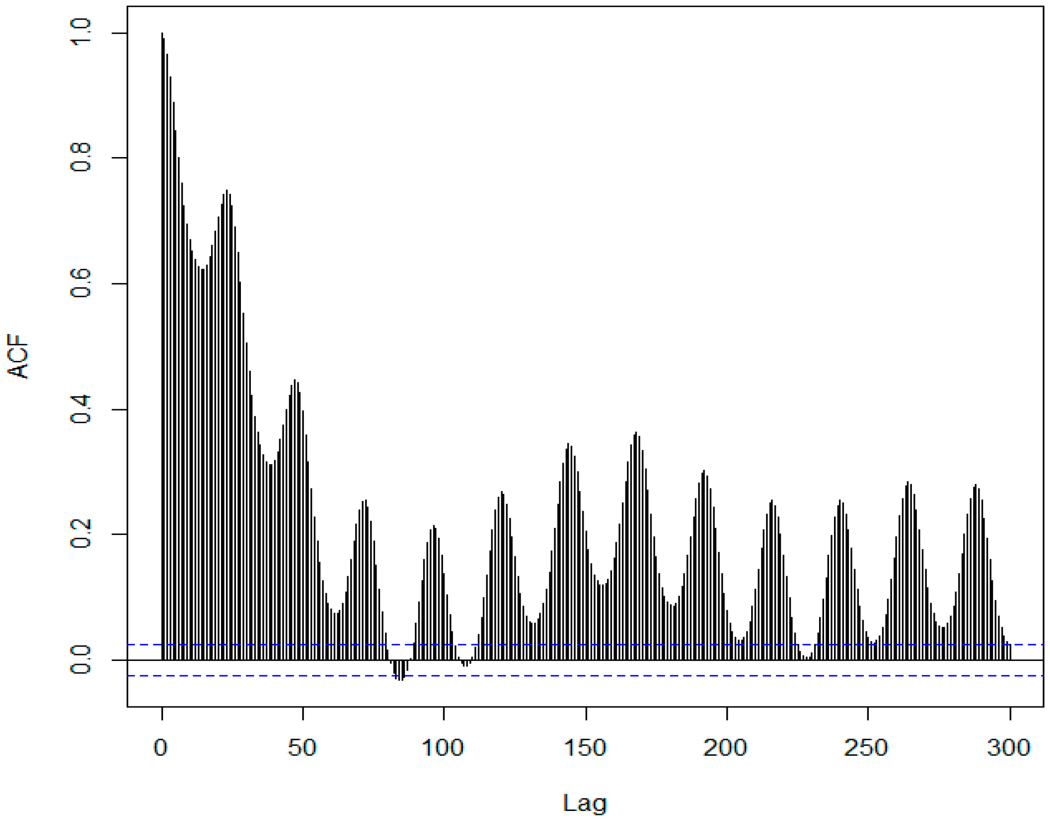
The summary statistics of the reconstructed calibration dataset are reported in Table 1. Figure 2 and Figure 3 report, respectively, the autocorrelation function and the histogram of the data. The correlogram reported in Figure 2 shows that there is a daily seasonality (lag = 24). In addition, a relative maximum is observed for lag = 168, meaning that a weekly seasonality could be explored as well.
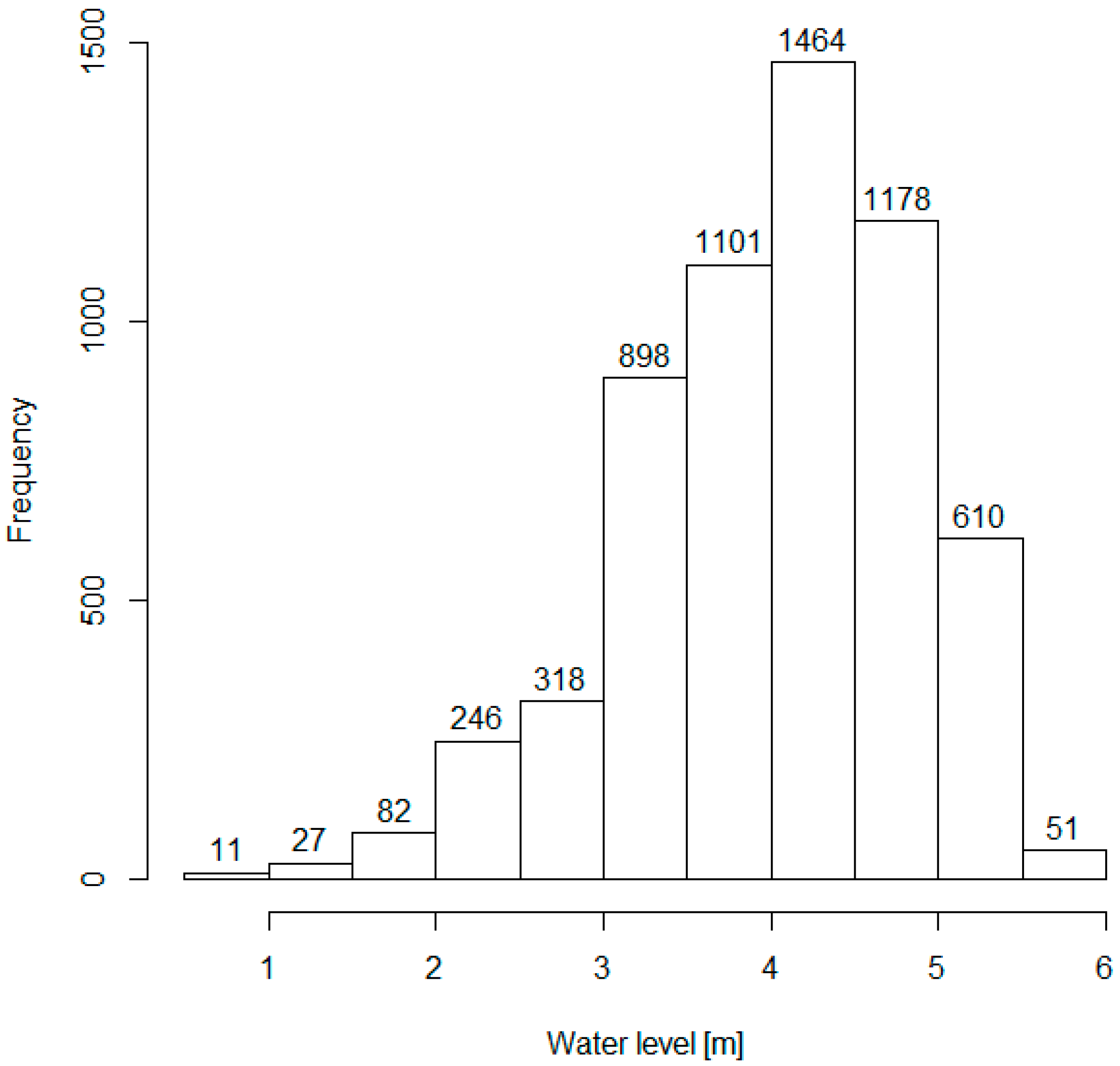
The distribution of the data reported in Figure 3 is skewed, due to the typical daily pattern of a water tank. The left tail has a low frequency occurrence because the situation of low storage in the tank is uncommon. A marked drop in frequency can be observed on the right side of the distribution, the range of water levels between 5 m and 6 m, because of the presence of the spillway, previously mentioned. The mode of the distribution is not centred but skewed to the right as the range 4–4.50 likely represents the optimal storage level at which the tank operates for water distribution.
4. ARIMA Model Calibration
As mentioned above, the adopted model is ARIMA (2, 1, 2). This model embeds a differentiation in the data of order 1. Autoregressive and moving average terms are included, both of them of order 2. The prediction provided by the model for a generic period t is described by the following equation:
This model provides one-step-ahead simulation.
Coefficients were estimated using the likelihood maximization as technique for parameter estimation, in the calibration dataset. Calculations have been performed by means of the statistical program “R”. Table 2 shows the estimated values of the coefficients of the model.
The plot of the estimated hourly water tank levels is reported in Figure 4. It can be noticed that the slope of the data is very similar to the one shown in Figure 1. The simulated data present a stationary behaviour in two time ranges, in the period 2194 to 2424 and the period 2527 to 2980. This is due to the fact that these ranges are the ones in which the dataset was reconstructed, imputing missing data with the DD-TSA model.
5. Results and Discussion
The ARIMA (2, 1, 2) model exhibits excellent performance when comparing the estimations with the measurements in the calibration dataset. Despite a few outliers, probably related to sudden spikes in the calibration dataset, the simulations are always very close to the measurements. This result can be quantitatively summarized in the residual analysis.
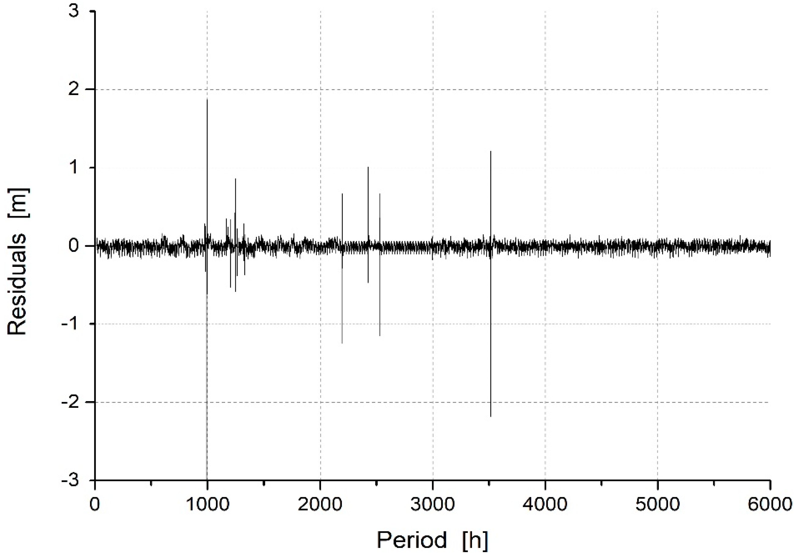
In Figure 5, the residuals of the model—the differences between the observed and simulated data—are plotted. Residuals larger than 0.5 m in absolute value are always related to periods in which the measurements were missing, and the estimated levels are compared with the imputations.
In Figure 6, a histogram of the residuals of the model is presented. A very narrow distribution of the residuals is obtained, as can be expected when looking at the plot in Figure 5, since the largest part of the data is gathered in a ±0.5 m interval with respect to zero. Basically, the model has very small residuals throughout the dataset, except for a few periods, corresponding to the imputed data.
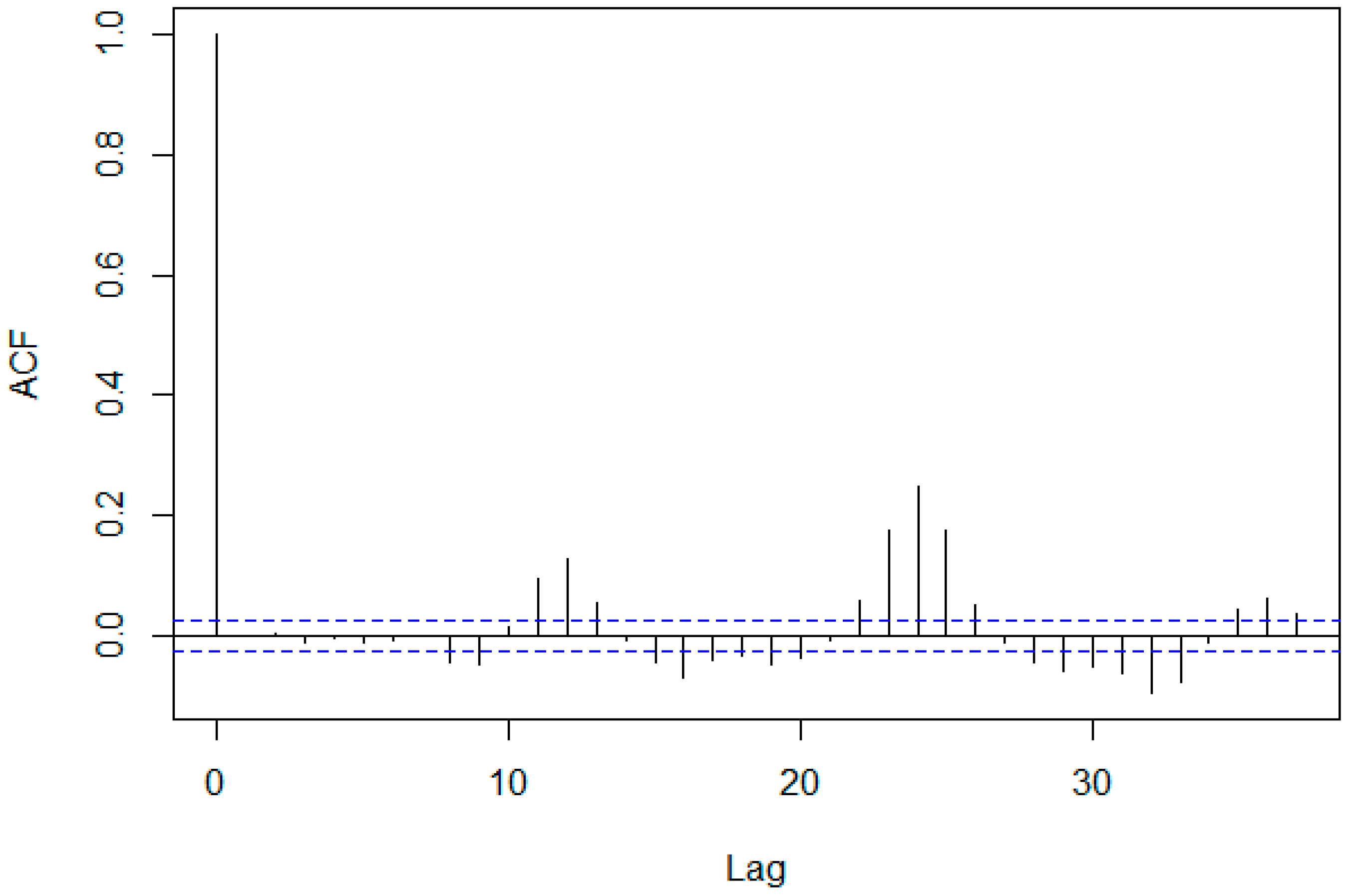
The autocorrelation of the residuals is shown in Figure 7. The values are very low, except for two relative maxima for lag = 12 and lag = 24. This result confirms the good performance of the ARIMA model and suggests further applications for which a seasonal model could be tested.
The statistics of the residuals are reported in Table 3. Besides the interesting result of very small mean and median values, it is valuable to confirm the presence of outliers by looking at the minimum and maximum values.
6. Conclusions
Today, in a context of water resource scarcity, optimal management is of paramount importance for the sustainable management of urban water networks. The management relies on water utility operations consisting of usually quick responses to either water demand or source variations as well as the effects of network aging.
In this framework, the present work aimed at the simulation of drinking water tank levels by time series analysis to support water distribution managers. The case study referred to the time series of the levels observed at the Gesuiti water tank, belonging to the water supply system of the town of Benevento, Italy. Since two large intervals of data were missing, data imputation was necessary to obtain a continuous series. This was achieved by the use of a preliminary DD-TSA model. ARIMA (2, 1, 2) was chosen as the optimal statistical model for the purpose, according to the BIC and DIC criteria.
The analysis of the model residuals showed a good agreement between the observed and simulated data. The residuals appeared with a zero mean value and a very moderate correlation at lag 12 and 24, which would suggest a seasonal component to be accounted for in the model description, which is foreseen in order to improve the data simulation for future applications.
Author Contributions
All authors have read and agreed to the published version of the manuscript. C.G., A.L., S.M. and G.V. conceived and designed the experiments; S.M. performed the experiments; C.G., A.L., S.M. and G.V. analysed the data and prepared the manuscript.
Funding
This research received no external funding.
Acknowledgments
The authors wish to thank GESESA S.p.A and Eng. Alessandro Gnerre for having provided the data.
Conflicts of Interest
The authors declare no conflict of interest.
References
- Bello, O.; Abu-Mahfouz, A.M.; Hamam, Y.; Page, P.R.; Adedeji, K.B.; Piller, O. Solving management problems in water distribution networks: A survey of approaches and mathematical models. Water 2019, 11, 562. [Google Scholar] [CrossRef]
- Viccione, G.; Ingenito, L.; Evangelista, S.; Cuozzo, C. Restructuring a water distribution network through the reactivation of decommissioned water tanks. Water 2019, 11, 1740. [Google Scholar] [CrossRef]
- Creaco, E.; Campisano, A.; Fontana, N.; Marini, G.; Page, P.R.; Walski, T. Real time control of water distribution networks: A state-of-the-art review. Water Res. 2019, 161, 517–530. [Google Scholar] [CrossRef] [PubMed]
- Madala, K.; Divya Bharathi, D.; Polavarapu, S.C. An internet of things for water utility monitoring and control. Int. J. Eng. Technol. 2018, 7, 20–23. [Google Scholar] [CrossRef]
- Koo, D.; Piratla, K.; Matthews, C.J. Towards Sustainable Water Supply: Schematic Development of Big Data Collection Using Internet of Things (IoT). Procedia Eng. 2015, 118, 489–497. [Google Scholar] [CrossRef]
- Candelieri, A. Clustering and support vector regression for water demand forecasting and anomaly detection. Water 2017, 9, 224. [Google Scholar] [CrossRef]
- Kang, D. Real-time optimal control of water distribution systems. Procedia Eng. 2014, 70, 917–923. [Google Scholar] [CrossRef]
- Tripathi, A.; Kaur, S.; Sankaranarayanan, S.; Narayanan, L.K.; Tom, R.J. Water demand prediction for housing apartments using time series analysis. Int. J. Intell. Inf. Technol. 2019, 15, 57–75. [Google Scholar] [CrossRef]
- Muhammad, A.U.; Li, X.; Feng, J. Artificial Intelligence Approaches for Urban Water Demand Forecasting: A Review. In International Conference on Machine Learning and Intelligent Communications; Zhai, X., Chen, B., Zhu, K., Eds.; Springer: Cham, Switzerland, 2019; Volume 294, pp. 595–622. [Google Scholar] [CrossRef]
- Zhao, L.; Zhang, J.; Chen, T. Application of product seasonal ARIMA model to the forecast of urban water supply. J. Water Resour. Water Eng. 2011, 22, 58–62. [Google Scholar]
- Billings, R.B.; Jones, C.V. Forecasting Urban Water Demand; American Water Works Association: Denver, CO, USA, 2008; ISBN 978-1-58231-537-1. [Google Scholar]
- Guarnaccia, C.; Tepedino, C.; Viccione, G.; Quartieri, J. Short-Term Forecasting of Tank Water Levels Serving Urban Water Distribution Networks with ARIMA Models. In Frontiers in Water-Energy-Nexus—Nature-Based Solutions, Advanced Technologies and Best Practices for Environmental Sustainability; Advances in Science, Technology & Innovation; Naddeo, V., Balakrishnan, M., Choo, K.H., Eds.; Springer: Cham, Switzerland, 2018. [Google Scholar] [CrossRef]
- Viccione, G.; Guarnaccia, C.; Mancini, S.; Quartieri, J. On the use of ARIMA models for short-term water tank levels forecasting. Water Supply 2020, 20, 787–799. [Google Scholar] [CrossRef]
- Viccione, G.; Pellecchia, V.; Parente, G. Una proposta per la riduzione delle portate di sfioro nei serbatoi di testata. In Proceedings of the VIII Seminario Tecnologie e Strumenti Innovativi per le Infrastrutture Idrauliche “TeSI”, Naples, Italy, 8–9 July 2019. [Google Scholar]
- Guarnaccia, C.; Quartieri, J.; Mastorakis, N.E.; Tepedino, C. Development and Application of a Time Series Predictive Model to Acoustical Noise Levels. WSEAS Trans. Syst. 2014, 13, 745–756. [Google Scholar]
- Guarnaccia, C.; Quartieri, J.; Rodrigues, E.R.; Tepedino, C. Acoustical noise analysis and prediction by means of multiple seasonality time series model. Int. J. Math. Models Methods Appl. Sci. 2014, 8, 384–393. [Google Scholar]
- Guarnaccia, C.; Quartieri, J.; Tepedino, C.; Rodrigues, E.R. A time series analysis and a non-homogeneous Poisson model with multiple change-points applied to acoustic data. Appl. Acoust. 2016, 114, 203–212. [Google Scholar] [CrossRef]
- Guarnaccia, C.; Mancini, S.; Quartieri, J.; Breton, J.G.C.; Breton, R.M.C. Prediction of CO concentrations in Monterrey, Mexico, by means of ARIMA models. WSEAS Trans. Environ. Dev. 2018, 14, 653–661. [Google Scholar]
Figure 1.
1-h averaged water tank levels, with evidence of missing data.

Figure 2.
Autocorrelation of the data as a function of the lag.

Figure 3.
Histogram of the data.

Figure 4.
Simulated hourly water tank levels, with ARIMA (2, 1, 2) model.

Figure 5.
Difference between observed and simulated hourly water tank levels.

Figure 6.
Histogram of the residuals of the ARIMA (2, 1, 2) model.

Figure 7.
Autocorrelation function (ACF) of the residuals of the ARIMA (2, 1, 2) model.


Table 1.
Descriptive statistics for the calibration dataset of water levels observed at the tank of Gesuiti.
Table 1.
Descriptive statistics for the calibration dataset of water levels observed at the tank of Gesuiti.
| Sample Size | Mean (m) | Std. Dev. (m) | Median (m) | Min (m) | Max (m) | Skewness | Kurtosis |
|---|---|---|---|---|---|---|---|
| 5986 | 4.00 | 0.85 | 4.12 | 0.87 | 5.72 | −0.63 | 0.28 |
Table 2.
Estimated coefficients of the ARIMA (2, 1, 2) model.
| Estimated Value | 1.7362 | −0.8146 | −1.1330 | 0.2334 |
Table 3.
Summary statistics of the residuals of ARIMA (2, 1, 2) model.
| Mean (m) | Std. Dev. (m) | Median (m) | Min (m) | Max (m) | Skewness | Kurtosis |
|---|---|---|---|---|---|---|
| 0.00 | 0.08 | 0.00 | −3.10 | 1.87 | −9.16 | 434.27 |
Publisher’s Note: MDPI stays neutral with regard to jurisdictional claims in published maps and institutional affiliations. |
© 2020 by the authors. Licensee MDPI, Basel, Switzerland. This article is an open access article distributed under the terms and conditions of the Creative Commons Attribution (CC BY) license (https://creativecommons.org/licenses/by/4.0/).
Share and Cite
MDPI and ACS Style
Guarnaccia, C.; Longobardi, A.; Mancini, S.; Viccione, G. Drinking Water Tank Level Analysis with ARIMA Models: A Case Study. Environ. Sci. Proc. 2020, 2, 33. https://0-doi-org.brum.beds.ac.uk/10.3390/environsciproc2020002033
AMA Style
Guarnaccia C, Longobardi A, Mancini S, Viccione G. Drinking Water Tank Level Analysis with ARIMA Models: A Case Study. Environmental Sciences Proceedings. 2020; 2(1):33. https://0-doi-org.brum.beds.ac.uk/10.3390/environsciproc2020002033
Chicago/Turabian StyleGuarnaccia, Claudio, Antonia Longobardi, Simona Mancini, and Giacomo Viccione. 2020. "Drinking Water Tank Level Analysis with ARIMA Models: A Case Study" Environmental Sciences Proceedings 2, no. 1: 33. https://0-doi-org.brum.beds.ac.uk/10.3390/environsciproc2020002033