
Determination of Satellite-Derived PM2.5 for Kampala District, Uganda


1
Department of Geomatics and Land Management, Makerere University, Kampala 7062, Uganda
2
Department of Computer Science, Makerere University, Kampala 7062, Uganda
*
Author to whom correspondence should be addressed.
Geomatics 2022, 2(1), 125-143; https://0-doi-org.brum.beds.ac.uk/10.3390/geomatics2010008
Submission received: 4 January 2022
/
Revised: 6 March 2022
/
Accepted: 7 March 2022
/
Published: 10 March 2022
Abstract
:Ground monitoring stations are widely used to monitor particulate matter (PM2.5). However, they are expensive to maintain and provide information localized to the stations, and hence are limited for large-scale use. Analysis of in situ PM2.5 shows that it varies spatially and temporally with distinct seasonal differences. This study, therefore, explored the use of satellite images (Sentinel-2 and Landsat-8) for determining the spatial and temporal variations in PM2.5 for Kampala District in Uganda. Firstly, satellite-derived aerosol optical depth (AOD) was computed using the Code for High Resolution Satellite mapping of optical Thickness and aNgstrom Exponent algorithm (CHRISTINE code). The derived AOD was then characterised with reference to meteorological factors and then correlated with in situ PM2.5 to determine satellite-derived PM2.5 using geographically weighted regression. In the results, correlating in situ PM2.5 and AOD revealed that the relationship is highly variable over time and thus needs to be modelled for each satellite’s overpass time, rather than having a generic model fitting, say, a season. The satellite-derived PM2.5 showed good model performance with coefficient of correlation (R2) values from 0.69 to 0.89. Furthermore, Sentinel-2 data produced better predictions, signifying that increasing the spatial resolution can improve satellite-derived PM2.5 estimations.
1. Introduction
Increased rates of urbanisation and population density have contributed to the high levels of air pollution in most cities and urban areas [1]. This is because urbanisation is characterized by high motor vehicle traffic and exhaust emissions, which are invariably responsible for high particulate matter concentrations and other severe environmental concerns in urban areas [2,3]. Particulate matter with a diameter less than 2.5 microns (PM2.5) has been identified as the leading air pollutant contributing to worldwide mortality rates and hence is a major threat to humans [4,5]. This is because these particles have a small diameter that is highly inhalable and thus they have been associated with several cardiovascular complications such as lung cancer, severe respiratory infections and stroke, which are more prominent among vulnerable groups such as children and the elderly [6,7,8,9]. Therefore, this conglomeration of factors has drawn the attention of many scholars, researchers and the public to address the issue of monitoring PM2.5.
Monitoring of PM2.5 has been mainly carried out using measurements from standalone devices or through a network of ground monitoring stations [10,11]. Ground stations offer two main advantages. Firstly, they can continuously measure pollution 24 h a day, providing average capacities hourly, daily, monthly or any time. Secondly, they can make observations under various environmental conditions [12]. In recent years, as in many African cities, there have been efforts to understand the state of urban air quality and exposure to PM2.5 concentrations in Kampala city using low-cost air quality sensors (LCAQS) [7,13,14]. Although LCAQS have become instrumental in monitoring PM2.5 concentrations in Kampala, they have not been fully utilised due to a lack of viable operating mechanisms and issues related to data gaps and data quality [15]. There is also still a scarcity of air pollution data and well-established ground station networks in most parts of Kampala District, resulting in hitches in understanding the spatial distribution of pollutant concentrations and trends [14]. Therefore, this paucity of information and the limited capacity to build efficient downstream data science applications have inspired the need to explore remote sensing techniques for monitoring PM2.5 [16]. Remote sensing provides a synoptic view of the regions, especially in the rural areas and developing countries, that may not have the capacity to build and maintain a dense ground station network [11]. Satellites operate by measuring aerosol properties, also known as the aerosol optical depth (AOD), which can be correlated with in situ PM2.5 to model satellite-derived PM2.5 [17,18,19].
The contributions of this article are, therefore, firstly, to provide an understanding of the spatial and temporal variations in aerosol optical depth, as well as its relationship with meteorological factors. Secondly, from the AOD characterisations, we modelled the relationship between AOD and in situ PM2.5, and used this relationship to estimate satellite-derived PM2.5. The rest of the article is structured as follows: the materials and methods are presented in Section 2, while results and discussions are in Section 3 and Section 4, respectively. Finally, Section 5 contains the conclusions and recommendations for future work.
2. Materials and Methods
2.1. Study Domain
The study focused on Kampala District because it is the capital city of Uganda and has the highest number of ground monitoring stations in the country. Kampala is about 189 km2 and is located in the central region of Uganda, where it experiences both the wet seasons from March to May (MAM) and September to November (SON), and the dry seasons from December to February (DJF) and June to August (JJA). According to census data projections [20], Kampala’s population was estimated to be 1,650,800 and this population has been projected to rise to about 1,927,400 by 2030 (reflecting a projected increment of approximately 7%). Kampala’s daytime population has also increased significantly to about 4.5 million due to the high number of commuters in the city [21]. This continuous increase in population density in the city has become one of the major driving forces of increased vehicle traffic and, consequently, increased exhaust fumes and smoke, resulting in increased contamination of outdoor air quality in the city. Kampala District has two local networks of ground PM2.5 monitoring stations coordinated by Kampala Capital City Authority (KCCA) and Makerere University in Uganda. The KCCA network (https://www.kcca.go.ug/kampala-air-quality-monitoring-network accessed on 10 April 2021) commenced operations in 2019 and currently operates 25 ground monitoring stations. The Makerere University network is coordinated by AIRQO (https://airqo.africa/ accessed on 15 April 2021), a university-based startup, and operates 17 monitoring stations. Apart from PM2.5, these stations also measure PM10 concentrations. In addition to the pollution monitoring stations, there are also 6 weather stations in each of the district’s divisions (Nakawa, Makindye, Central, Kawempe and Rubaga divisions) that are responsible for monitoring the meteorological conditions in the area. These weather stations are coordinated by the Trans-African Hydro-Meteorological Observatory (TAHMO) initiative (https://portal.tahmo.org/ accessed on 15 April 2021). Figure 1 shows the location of Kampala District and the distribution of PM2.5 monitoring stations and meteorological stations.
2.2. Data
2.2.1. In Situ PM2.5 Data
In situ PM2.5 data were collected from the ground monitoring stations for the period from January 2019 to March 2021. Kampala District has a number of static low-cost pollution monitors deployed on permanent structures such as buildings and poles. These monitors have been locally and uniquely designed to withstand various environmental and physical conditions. The devices measure PM2.5 concentrations using nephelometer (light-scattering) technology (with a dual plan-tower PMS5003 sensor) that has an effective measurement range of 0–500 μg/m3 [15]. These ground monitoring stations collect data every 90 s, which is transmitted in real-time via a local global system for mobile communications (GSM) to a cloud-based platform [15]. This real-time transmission of data provides an effective mechanism for monitoring and managing public health and environmental issues. Moreover, the devices operate on solar energy and collect the location data (latitude, longitude) of the monitoring stations.
2.2.2. Satellite Data
The study made use of the Landsat-8 and Sentinel-2 satellite images that are freely available and can be downloaded from the USGS-earth explorer website (https://earthexplorer.usgs.gov/ accessed on 5 April 2021). The Landsat-8 satellite circles the Earth in a sun-synchronous orbit with a repeat cycle of 16 days [22,23]. It was launched in 2013 and carries onboard the Operational Land Imager (OLI) instrument with 9 spectral bands and a thermal infra-red sensor with two thermal bands (Band 10 and 11) [23,24]. The satellite has a swath width of approximately 183 km [25]. On the other hand, the Sentinel-2 satellite comprises a constellation of two twin polar-orbiting satellites (Sentinel-2A and Sentinel-2B) placed in the same sun-synchronous orbit [26]. Sentinel-2 satellites have a swath width of 290 km and a high revisit time (i.e., 10 days at the equator with one satellite, and 5 days with 2 satellites, resulting in 2–3 days at mid-latitudes) [23]. Sentinel-2 satellites carry a Multi-Spectral Instrument (MSI), which samples 13 spectral bands with spatial resolution ranging from 10 m to 60 m [26].
Estimation of AOD from these satellite images is highly dependent on the availability of cloud-free images; therefore, cloud-free images or those with limited cloud cover coverage in the study area were selected for use in this study. Fifty-three Sentinel-2 and Landsat-8 images were downloaded for the period of 2019–2021. However, only the 9 images with the least cloud cover were retained for use in this study. The selection of this study period (i.e., 2019–2021) was based on when ground monitoring of PM2.5 concentrations commenced in Kampala District.
2.2.3. Meteorological Data
Meteorological parameters were accessed from the 6 weather stations in Kampala District. The data used from these stations were filtered to coincide with the satellite overpass time (i.e., 8:20 UTC and 8:00 UTC for Sentinel-2 and Landsat-8, respectively).
2.3. Methods
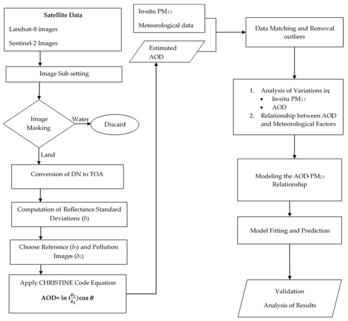
In this study, we used the Code for High Resolution Satellite mapping of optical Thickness and aNgstrom Exponent algorithm (CHRISTINE code) [27] to retrieve the AOD from the satellite images and performed a hotspot analysis to evaluate the spatial and temporal variations in AOD. To estimate the satellite-derived PM2.5, firstly, the AOD was correlated with in situ PM2.5 and additional parameters of the meteorological data. Geographically weighted regression (GWR) was then applied to the AOD–PM2.5 relationship to determine the satellite-derived PM2.5. Figure 2 shows the flow chart for the methodology used to achieve the study objectives.
To retrieve the AOD, satellite images were first prepared by calibrating the images’ digital number values to the top of atmosphere (TOA) reflectance, and then the reflectance standard deviations were computed.
2.3.1. Conversion of Digital Number to TOA Reflectance
Sentinel-2 Level 1C data are provided as a TOA product. The Landsat-8 imagery, on the other hand, needed calibration of the DN values to TOA reflectance using Equation (1):
where Lλ is the TOA reflectance, ML is the band-specific multiplicative rescaling factor from the metadata (RADIANCE_MULT_BAND_X, where X is the band number), AL is the band-specific additive rescaling factor from the metadata (RADIANCE_ADD_BAND_X, where X is the band number), QCAL is the quantized and calibrated standard product pixel values (DN) and ⊖ is the scene centre’s sun elevation angle in degrees provided in the metadata (SUN_ELEVATION).
Lλ = MLQCAL + AL/sin⊖
2.3.2. Computation of Reflectance Standard Deviations
Reflectance standard deviations are major inputs into the CHRISTINE code to retrieve the AOD from satellite images. The algorithm uses a contrast reduction principle over a computational grid superimposed onto the satellite images [27]. In this study, computational grid sizes of 17 by 17 pixels and 6 by 6 pixels were used for Sentinel-2 and Landsat-8 images, respectively. Different grid sizes were used to ensure that the area covered by the computational grid in both sensors was comparable. The use of standard deviations in the computation of AOD aimed at modelling the spatial correlation of AOD within the study area.
2.3.3. Estimation of Aerosol Optical Depth (AOD)
Selection of Reference and Pollution Images
The CHRISTINE code algorithm requires the selection of reference and pollution images. The reference image refers to the image with the lowest PM2.5 concentration as recorded by the ground monitoring stations. The reference image should also be cloud-free or have the lowest percentage of cloud cover, with known and available meteorological data [28]. On the other hand, the pollution image represents the image date for which the pollution data are to be determined. In light of these prerequisites, the Landsat-8 and Sentinel-2 images collected on 5 January 2019 were selected as the reference images. Reference images were selected for each sensor to eliminate errors and biases that may have arisen due to differences in sensor geometries and resolutions. Table 1 shows the particulars of the selected pollution and reference images used in this study.
Retrieval of AOD
AOD was determined by applying the CHRISTINE Code equation (see Equation (2)) to the selected reference and pollution images. In this study, the green band was used because the effects of atmospheric aerosols are stronger and more easily perceived than other wavelengths and hence, they are the best for AOD retrieval [27,28]. Additionally, the green band is not obfuscated by the substantial molecular optical thickness and is sensitive to the presence of inhalable fine particles with a size of around 2 mm [27,28]. For each of the selected images, the satellite-derived AOD was computed, and the resulting AOD maps were classified according to the AOD classification classes defined by [27].
∆τ = ln [δ₁/δ₂] cos⊖v
2.3.4. Data Matching and Integration
All the datasets (i.e., in situ PM2.5 concentrations, meteorological data and derived AOD) were transformed into the WGS84 geographic coordinate system. The datasets were then matched both spatially and temporally to reduce the impact of data noise and spatial instability in the subsequent analysis [29]. Since the meteorological data and in situ PM2.5 concentrations were acquired from different monitoring stations, the PM2.5 monitoring sites were spatially linked to the nearest meteorological station. As a result, the in situ PM2.5 concentrations and meteorological data were then registered into the same monitoring site and thus, spatial matching of datasets collocated the variables to the PM2.5 ground receiving stations. On the other hand, temporal matching involved the extraction of PM2.5 concentrations and meteorological variables coincident with the satellite overpass time. Additionally, extreme (outliers) and nominal values of both the AOD and PM2.5 concentrations were also eliminated.
For the daily PM2.5 concentrations, the number of daily records is a vital consideration to ensure the accuracy of GWR modelling [30]. From our preliminary trials, the daily threshold of 30 records that were within a period 30 min before and after the satellite overpass time were manually selected to ensure a sufficient number of validated daily records. The average of these records was used as the station’s PM2.5 measurement record at each image acquisition date (satellite overpass time). For the Sentinel-2 and Landsat-8 AOD products, insignificant pixel values (i.e., in the range of 0 to 0.05), mainly due to cloud cover, were also excluded from the data subsets to reduce noise and bias in GWR modelling. However, this can greatly reduce the number of validated records for GWR modelling [30].
2.3.5. Analysis of In Situ PM2.5 and AOD Variations
Following the computation of AOD for all the years in the study period, characterisation of the variations in in situ PM2.5 and AOD was carried out. This analysis was carried out by evaluating the trends in the in situ PM2.5 concentrations and satellite-derived AOD. Moreover, the relationship between AOD and environmental factors (meteorological variables) was evaluated through linear and nonlinear relationship techniques. The spatial characterisation was carried out through hotspot analysis to determine areas of high aerosol concentrations and those with a low aerosol content. Characteristics of the locations for the identified hotspot areas were also evaluated to better understand the aerosol concentrations in these areas.
2.3.6. Estimation of PM2.5 Concentrations
Having estimated the AOD and analysed its variations, the next step was to determine PM2.5 using the relationship between AOD and in situ PM2.5 measurements. Firstly, the AOD–PM2.5 relationship was modelled using two model setups, i.e., seasonal and time-specific models. Modelling the AOD–PM2.5 relationship under the two model setups was carried out through multiple regression analysis. The adjusted R2 and the multiple correlation coefficient in each of the setups were used as measures of the strength of the relationship. Finally, an analysis of these statistics (i.e., the correlation coefficient and adjusted R2) was carried out. The model setup with the highest correlation coefficient and adjusted R2 values was chosen to estimate the satellite-derived PM2.5.
The data were randomly divided into two subsets, i.e., 80% for model fitting and prediction, and 20% of the data for validation of the results. Next, the geographical weighted regression in Equation (3) was applied to estimate the satellite-derived PM2.5 concentrations over the study area.
where PM2.5s represents the daily PM2.5 concentration at location s(i, j), b0 and b1–bn denote the intercepts and slopes for each independent variable (AOD, temperature (TEMP), relative humidity (RH), air pressure (AP) and wind speed (WS)) and ε stands for the error term.
PM2.5s = b0(i,j) + b1(i,j)AOD + b2(i,j)TEMP +… + bn(i,j)WS + ɛs
The GWR model was used due to its ability to estimate PM2.5 distributions on a large scale, and to examine the spatial variability and nonstationarity of variables [31]. GWR was also selected because it requires fewer data compared with other models such as machine learning algorithms [32]. This factor was especially crucial in this study, given the limited number of PM2.5 ground monitoring stations in the study area.
Validation of the estimated PM2.5 was determined using the coefficient of correlation between the predicted and observed values. Moreover, the root mean square error (RMSE) values were computed and used to assess the degree of variation between the observed and predicted PM2.5 values.
3. Results
3.1. Analysis of In Situ PM2.5
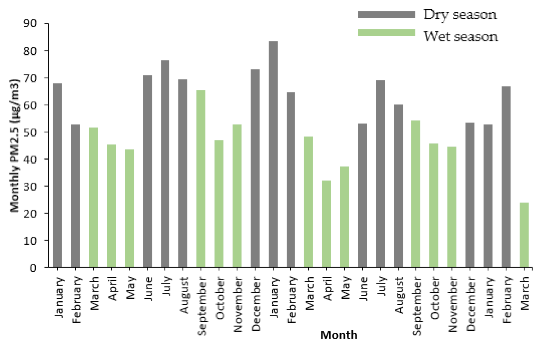
Figure 3 shows the averages of the monthly in situ PM2.5 concentrations recorded by the measuring stations within the study period. From Figure 3, it is evident that the lowest PM2.5 concentrations occurred within the wet-season months of April, May, October and November. Whereas at the beginning of the wet season, PM2.5 concentrations were relatively high (March for MAM and September for SON), they showed a declining trend in PM2.5 heading into the wet season. Conversely, the highest PM2.5 concentrations occurred during the dry months of December, January, February, June, July and August (DJF and JJA). These observations illustrate the clear seasonal cycle experienced in the study area, with notably high PM2.5 during the dry seasons and low PM2.5 concentrations during the wet seasons.
3.2. Variations in AOD
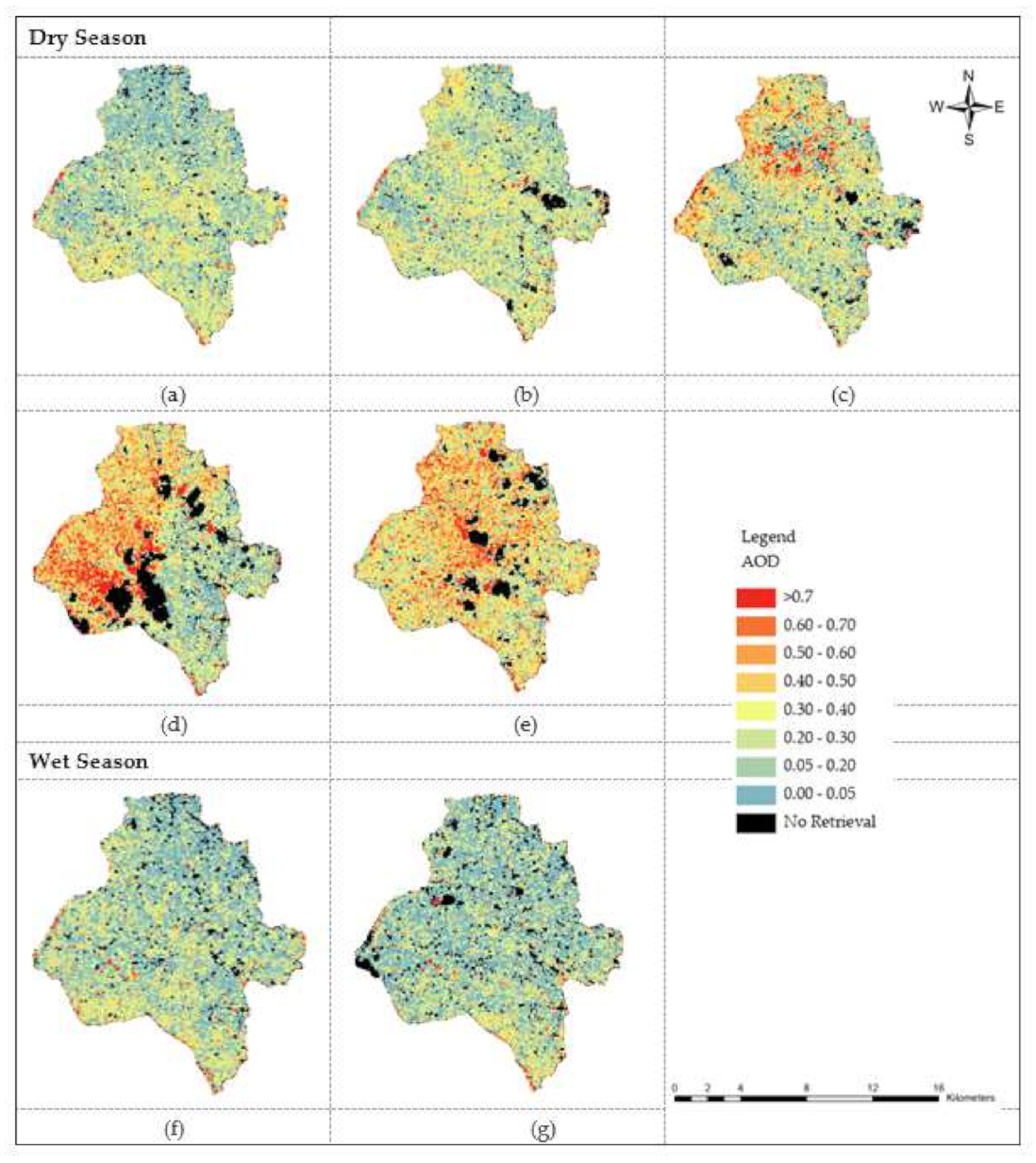
Having examined the seasonal cycle of ground PM2.5 concentrations, we then set out to determine if the satellite-derived AOD and the consequently derived PM2.5 captured these instances. Figure 4 shows the results of AOD retrieval for the selected images over the study area.
AOD is a dimensionless quantity, and the measurements were classified into AOD classes, including the “no retrieval class” as defined by [27]. The “no retrieval” class is also referred to as the unclassified class and represents areas where the CHRISTINE code decision criteria based on the Ångstrom power-law could not identify and isolate the reductions in contrast; hence the AOD values could not be computed in these areas [27]. Therefore, the “no retrieval” class includes areas such as those affected by cloud cover, since such areas exhibit very low contrast. Furthermore, the CHRISTINE code is restricted to highly contrasted areas.
From the seasonal patterns observed in the ground-based PM2.5 observations, satellite images acquired in the months of December, January and February lie within the dry season, while those acquired in September and March lie in the wet season. Therefore, to understand variations in the AOD estimates, the changes in aerosol concentrations were analysed temporally (for the dry and wet seasons) and spatially. The temporal/seasonal analysis of AOD variations showed that, in general, the highest aerosol loading was experienced in the dry season and the lowest aerosol concentrations were in the wet season, as shown in the images acquired in these seasons (Figure 4). This, therefore, shows that satellite observations are able to depict the seasonal dynamics of the observations from the ground monitoring stations.
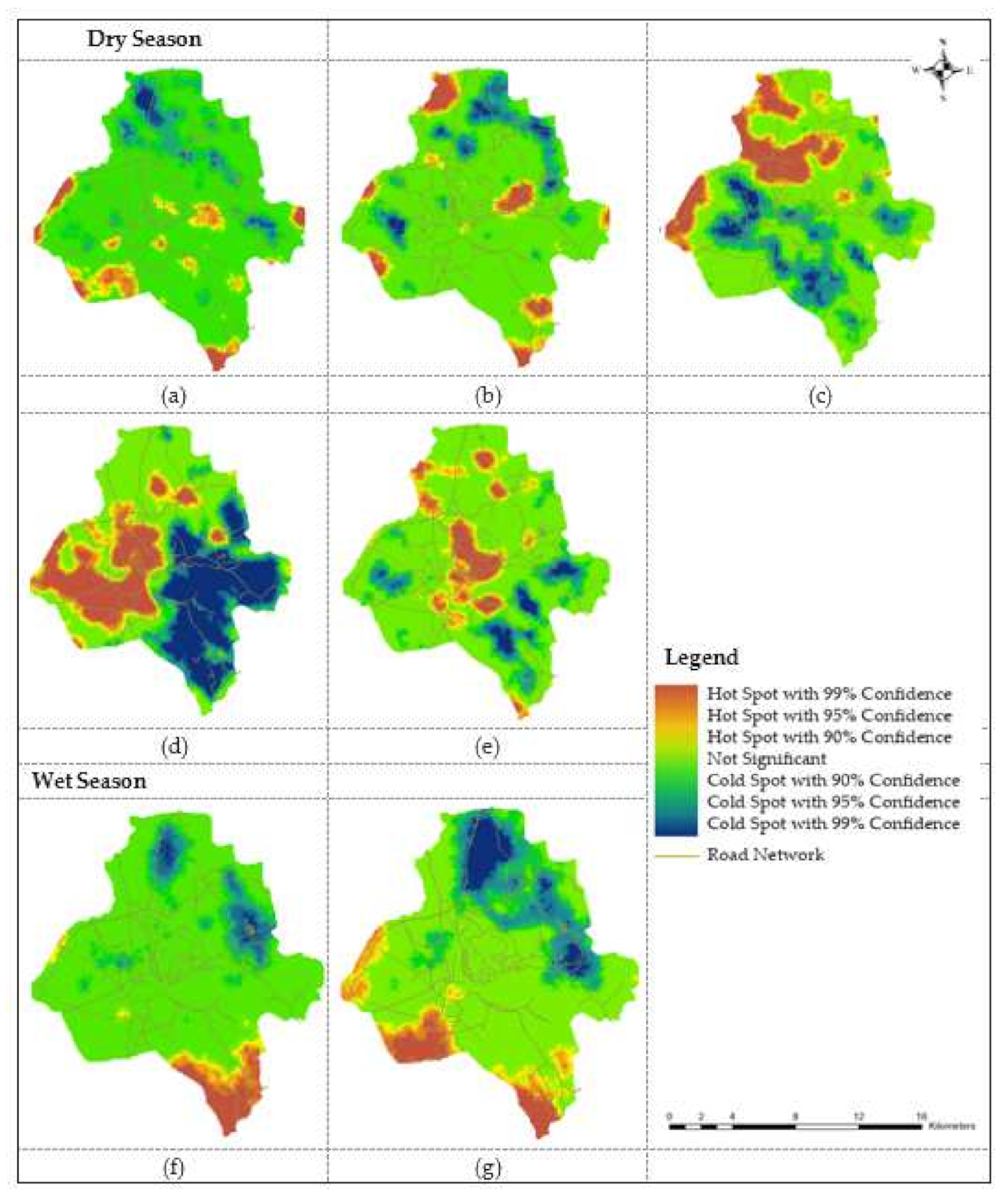
Analysing the spatial variations in AOD was achieved through the identification of major AOD hotspot areas in the study area. The results revealed that the AOD measurements varied spatially throughout the study period, as seen in Figure 5. Therefore, the hotspot areas’ spatial distribution and location were not constant over the entire study period. These areas were observed to be at varying locations for each image acquisition date. This is due to the varying anthropogenic activities or pollution sources in the different locations in the study area at the time of satellite overpass. Figure 5 also reveals that with satellite measurements, both the hotspots’ locations and extents can be captured at the time of satellite overpass as compared with in situ measurements, where the identification of hotspots and their spatial distribution are limited to the locations of the monitoring stations.
3.3. Relationship between AOD and Meteorological Factors
Satellite observations (aerosol properties) were taken under various environmental and meteorological conditions. Therefore, to evaluate and understand the variations in AOD, these factors need to be considered. Moreover, temporal analysis of the variations in in situ PM2.5 and AOD concentrations revealed seasonal patterns, and hence the relationship between AOD and meteorological factors was also evaluated on the basis of the two seasons experienced in Kampala District. For this analysis, the data variables were thus aggregated into two seasons.
3.3.1. Wet Season
Analysis of the relationship between the AOD and the meteorological variables was carried out through linear and nonlinear regression analysis. The linear regression analysis (Table 2) showed that there is generally a poor linear relationship between AOD and meteorological variables, as revealed by the weak linear coefficients of correlation (R).
Further analysis using the nonlinear relationship showed an improvement in the relationship, as shown by the nonlinear correlation coefficients, indicating that their relationship is nonlinear.
3.3.2. Dry Season
In the dry season, the linear relationship between AOD and meteorological factors (Table 3) showed an improvement in the correlation coefficients compared with the wet season. Wind speed was observed to have a positive correlation with AOD, indicating that an increase in wind speed increases the amount of aerosols in the atmosphere. Air pressure and relative humidity showed weak negative and positive correlation coefficients with AOD, respectively, indicating that they have small and insignificant linear influences on the variations in atmospheric aerosols. Similarly, temperature showed no linear relationship with AOD concentrations.
A nonlinear evaluation of this relationship using the Random Forest algorithm also showed a significant improvement in the nature and strength of the relationship (as shown by the nonlinear correlation coefficient, R).
3.4. PM2.5 Estimation
The relationship between AOD and in situ PM2.5 was used to estimate satellite-derived PM2.5 concentrations. From an analysis of the variations in in situ PM2.5 concentrations and AOD, it was revealed that the measurements have a seasonal pattern and hence need to be accounted for when modelling the AOD–PM2.5 relationship.
3.4.1. Modelling the AOD–PM2.5 Relationship
Modelling of the AOD–PM2.5 relationship was based on two model setups i.e., the seasonal and time-specific models. Evaluation of these model setups based on the correlation coefficients and adjusted R2 values was carried out to select the model that best represents the relationship.
The seasonal model setup modelled the AOD–PM2.5 relationship for the dry and wet seasons by aggregating all data into the two seasons, i.e., the dry and wet seasons. The results in Table 4 show that the AOD–PM2.5 relationship varied across the wet season and dry season, with correlation coefficients (R) of 0.58 and 0.40 for the wet and dry seasons, respectively. These correlations are, however, weak, implying that much of the variation in the PM2.5 concentrations cannot be explained by the AOD and meteorological factors when the data are aggregated into longer periods (seasons). From the adjusted R2 values, it can also be observed that these variables (AOD and meteorological factors) could explain 10% and 25% of the variations in PM2.5 with the seasonal model setup for the dry season and wet season, respectively.
With the time-specific model setup, the data were disaggregated into individual days, i.e., at each satellite overpass time, rather than aggregating the data into seasons. As a result, a general improvement in the strength of the AOD–PM2.5 relationship shown by the correlation coefficients (R) and adjusted R2 was observed, as seen in Table 5. The results indicate that considering the time-specific measurements minimises the effects of environmental changes such as land cover changes on the AOD–PM2.5 relationship, since the measurements are over a short period. This is also because AOD is a columnar measurement that is taken under the influence of various atmospheric and weather conditions that vary over shorter periods; hence, the time interval components need to be accounted for.
Therefore, compared with the seasonal model setup, the time-specific model setup yielded better relationships between AOD and in situ PM2.5, and thus was adopted in the subsequent processes of estimating PM2.5 concentrations from satellite observations.
3.4.2. Model Fitting
The relationship between the AOD and in situ PM2.5 at each satellite overpass time was used to estimate the PM2.5 concentrations by applying geographically weighted regression. The relationship at each satellite overpass time was used to reduce the biases resulting from the seasonal differences because the AOD and PM2.5 were observed to vary rapidly over short time intervals. The model estimation results show that the model performed considerably well at predicting PM2.5 concentrations for each of the time-specific image acquisition dates (satellite overpass time) over the study period, with R2 values ranging from 0.69 to 0.89, as seen in Table 6. This also means that the variables could explain much of the variability (i.e., 69% to 89%) in the PM2.5 concentrations. Since the data were divided into two subsets, i.e., 80% for model fitting and 20% for validation, PM2.5 estimation for the satellite overpass time of 31 December 2019 was eliminated because of the limited in situ observations for both model fitting and validation.
3.5. Validation
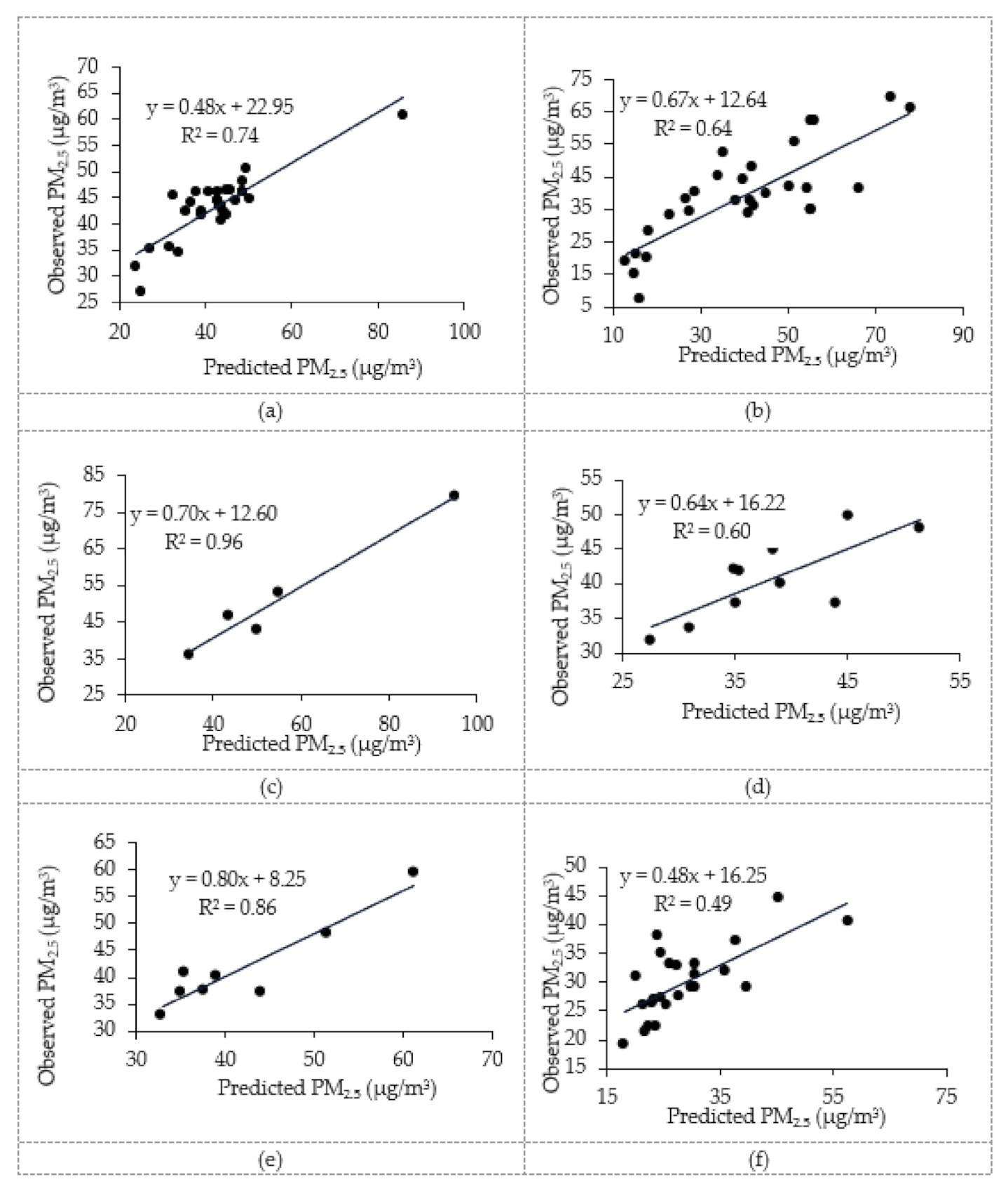
The validation results in Figure 6 show a moderately good agreement between the observed (in situ) and predicted PM2.5 values.
From Figure 6, it can be seen that the R2 values were affected by sample size; therefore, the root mean square error (RMSE) values were computed and used to assess the accuracy of the results (Table 7). The results show that the RMSE values at each satellite overpass time throughout the study period were lower than the minimum observed PM2.5 values, indicating that the satellite-derived PM2.5 values represent the ground measurements [33].
Moreover, since images from two sensors (i.e., Sentinel-2 and Landsat-8) were used in this study, the sensors’ performance was evaluated using images taken on the same day, and only 9 February 2020 date a matching set of images. The time lag between the Sentinel-2 and Landsat-8 overpass times in Kampala is approximately 18 min, and this accounts for the variation in the in situ PM2.5 concentrations. Due to the high variability in PM2.5 concentrations, a considerable difference was observed in situ, as seen in Table 8.
Table 8 shows that both the prediction and validation models performed better when using Sentinel-2 data products, with an RMSE of 8.53 μg/m3 compared with the Landsat-8 data with an RMSE of 13.38 μg/m3
3.6. Distribution of Derived PM2.5 Concentrations
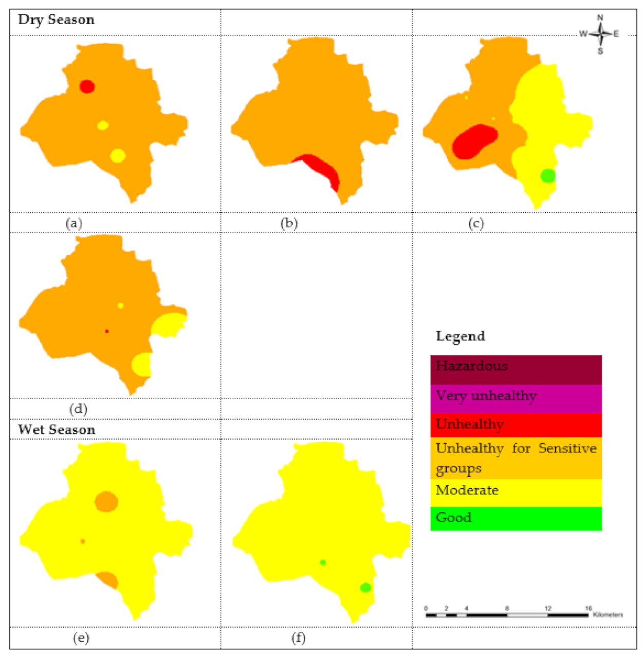
For the distribution of PM2.5 estimates, the inverse distance weighting (IDW) interpolation technique was used to generate a surface representing the distribution of PM2.5 estimates for Kampala. The concentration estimates (satellite-derived PM2.5) were categorised as per the Environmental Protection Agency (EPA) Air Quality Index (AQI) scale, as shown in Figure 7. Similar to the ground PM2.5 observations, the estimated PM2.5 results showed that the concentrations were high (generally unhealthy for sensitive groups) in the dry season months compared with the wet season months (i.e., the have generally moderate concentrations). This also depicts the seasonal patterns in satellite-derived PM2.5 that were observed with the in situ PM2.5 measurements and the satellite AOD.
4. Discussion
In the in situ results, the PM2.5 measurements varied spatially and temporarily, with a distinct seasonal pattern. The assessment of the satellite-derived AOD and the subsequently derived PM2.5 showed that these spatial and temporal nuances can be accurately captured. Analysing both the in situ PM2.5 and AOD variations revealed that the highest aerosol loading was experienced in the months of December, January and February, which are within the dry season. This is because the dry season is composed of high temperatures, resulting in uneven heating and temperature differences that facilitate increased chemical reactions and turbulence between particles, leading to the accumulation and formation of secondary aerosols in the atmosphere [34]. On the other hand, low AOD and in situ PM2.5 values were observed in the months of March, April, May, September and November, which are within the wet season that has a high moisture content. During the wet season, the high moisture content holds the aerosols together and as the moisture increases, the droplets fall to the ground. Hence, the aerosol load is very low due to the increased washing-off effect of the rain [35]. Additionally, analysis of the spatial variations in the AOD showed that the aerosol concentrations varied spatially, with high AOD (hotspots) concentrations along transport routes and road junctions and their surrounding environs. This pattern is similar to the temporal and spatial distribution of aerosol concentrations reported by [7,14]. The high levels of aerosol loading along major transport routes, junctions and city centres resulted from heavy vehicle traffic emissions, especially during the rush hours [36]. Moreover, along transport routes, dust is blown by moving vehicles, thus contributing to the high levels of aerosol concentrations in the lower atmosphere. This therefore implies that the characteristics of the locations and anthropogenic activities are responsible for the spatial distribution and amount of aerosol content in the area.
To precisely characterise the variations in the satellite observations, meteorological factors were also considered. Analysis of the relationship between the AOD and the meteorological variables for the wet season revealed that there is generally a poor linear relationship between the AOD and the meteorological variables. This is because the meteorological factors vary significantly over a short period, thus exerting both positive and negative influences on the variations in AOD over time. This, therefore, suggests that the relationship is nonlinear, as evidenced by the strong nonlinear coefficients of correlation, and thus may not be explained by linear relationships [37]. In the dry season, the linear relationship between AOD and meteorological factors was observed to be very poor for air pressure, relative humidity and temperature, similar to the case of the wet season, but with an improvement in the correlation coefficient for wind speed. This is because wind speed creates favourable conditions for the diffusion process of aerosol concentrations and increases the blowing-off effect, thus indirectly increasing the accumulation of aerosol concentrations in the atmosphere [35]. Conclusively, the most dominant factor affecting the aerosol variations in Kampala District is wind speed. Whereas poor linear relationships were observed between the AOD and meteorological variables, strong nonlinear relationships were observed, as shown by the nonlinear coefficients of correlation. These findings, therefore, indicate that meteorological factors exert both positive and negative impacts (complex relationships) on the variations in AOD, depending on the changes in environmental conditions and seasons, and thus cannot be explained using linear relationships [38].
In modelling the AOD–PM2.5 relationship, the R2 values and correlation coefficients were lowest for the seasonal model as compared with the time-specific model. This may be attributed to the observational noise arising from land-use changes, atmospheric reactions and other environmental changes that could have taken place between the months considered, since all data were aggregated into the two seasons experienced in the study area. These changes, in turn, lead to variations in the composition of atmospheric particles that further affect the aerosol concentrations and the AOD–PM2.5 relationship [35]. Hence, much of the variation in PM2.5 for the dry and wet seasons could not be easily explained by the aggregated AOD and meteorological data. This also implies that the AOD–PM2.5 relationship is affected not only by meteorological factors but also by the cumulative effects of various environmental factors over the proceeding days [34]. However, with the time-specific model setup, an improvement in the correlation statistics (higher correlation coefficients and R2 values) for the AOD–PM2.5 relationship was observed. This is because the time interval between the acquisition times for the measurements considered in this relationship was reduced. Therefore, the impact of environmental changes such as land-use changes was minimised. Hence, the variables could explain more of the variations in PM2.5 compared with the seasonal model and thus this model setup was adopted to estimate the PM2.5 concentrations for Kampala District.
GWR was then used to estimate the satellite-derived PM2.5, and an assessment of the model’s performance revealed that compared with in situ PM2.5, R2 ranged from 0.69 to 0.89. According to the R2 and RMSE, the estimated PM2.5 results were comparable with the in situ data measurements, showing that the satellite measurements represented the ground observations. Similar to the in situ PM2.5 variations, the distribution of the estimated PM2.5 showed that high (unhealthy concentrations) PM2.5 estimates are experienced in the dry season and low PM2.5 concentrations (moderate concentrations) in the wet season. The distribution of estimated PM2.5 showed that high PM2.5 estimates are found along transport routes, implying that the primary sources of PM2.5 are vehicle exhaust fumes and secondary particles such as sulphates and nitrates from chemical reactions between particles in the atmosphere. This spatial distribution of estimated PM2.5 also reveals that local anthropogenic emissions and activities are responsible for most of the air pollution concentrations within Kampala District.
Validation of these results showed that the predictions made from Sentinel-2 data had minimal variations from the in situ measurements compared with those from Landsat-8 data. This means that Sentinel-2 data products can predict PM2.5 concentrations with much higher accuracy and consistency. This was attributed to the higher spatial resolution of Sentinel-2 (i.e., a spatial resolution of 10 m) compared with 30 m for Landsat-8. Therefore, the spatial resolution of a sensor can potentially improve the prediction accuracy of PM2.5 concentrations.
5. Conclusions
Sentinel-2 and Landsat-8 images were used in this study to derive the AOD and subsequently estimate the satellite-derived PM2.5 of Kampala District. Modelling of the AOD–PM2.5 relationship revealed that the relationship varies across time, depending on the prevalent environmental conditions and is stronger when shorter periods are considered. This implies that best results will be achieved when AOD–PM2.5 is modelled on the basis of satellite overpasses rather than modelling the relationship across longer time periods such as seasons.
The predicted PM2.5 results were found to be comparable with in situ data measurements, showing that satellite measurements can be modelled accurately to represent ground observations. It was also observed that increasing the spatial resolution potentially increases the estimation accuracy of satellite-derived PM2.5 concentrations.
With the advent of UAV technology, targeted monitoring could be explored at the identified hotspot areas for further assessment and timely intervention at a much higher spatial resolution. This could also counter the effect of cloud cover, which is a significant limitation to using satellite images with low and medium spatial resolution. The study also recommends upscaling of the research to analyse the regional PM2.5 mass concentrations and determine the major contributors to the regional air pollution concentrations. Although satellite data are instrumental in monitoring and complementing in situ PM2.5 measurements, the estimates are limited to the satellite overpass times. Cloud cover and limited in situ PM2.5 measurements were the main challenges affecting the accuracy of estimating PM2.5 concentrations from satellite observations.
Author Contributions
Conceptualization, C.A. and A.G.; data curation, C.A.; formal analysis, C.A.; funding acquisition, A.G.; investigation, C.A.; methodology, C.A.; project administration, A.G.; resources, E.B. and A.M.; software, A.M.; supervision, A.G. and E.B.; validation, C.A.; visualisation, C.A. and A.G.; writing—original draft, C.A.; writing—review and editing, C.A., A.G., E.B. and A.M. All authors have read and agreed to the published version of the manuscript.
Funding
This research was funded by the RCMRD/GMES and Africa Research grant.
Institutional Review Board Statement
Not applicable.
Informed Consent Statement
Not applicable.
Data Availability Statement
Remote sensing data (both Landsat-8 and Sentinel-2) can be accessed from the USGS website (https://earthexplorer.usgs.gov/ accessed on 5 April 2021). The meteorological data were retrieved from the six weather stations of the Trans-African Hydro-Meteorological Observatory (TAHMO) Network (https://portal.tahmo.org/ accessed on 15 April 2021). Finally, the in situ PM2.5 data were obtained from the ground monitoring stations managed by AirQO (https://airqo.africa/ accessed on 15 April 2021) and Kampala Capital City Authority (https://www.kcca.go.ug/kampala-air-quality-monitoring-network accessed on 10 April 2021).
Acknowledgments
The authors would like to acknowledge the comments from the anonymous reviewers, whose contribution has gone a long way to improving the original draft.
Conflicts of Interest
The authors declare no conflict of interest.
References
- Fernández-Pacheco, V.M.; López-Sánchez, C.A.; Álvarez-Álvarez, E.; López, M.J.S.; García-Expósito, L.; Yudego, E.A.; Carús-Candás, J.L. Estimation of PM10 Distribution using Landsat5 and Landsat8 Remote Sensing. Proceedings 2018, 2, 1430. [Google Scholar] [CrossRef] [Green Version]
- Jiang, Q.; Christakos, G. Space-time mapping of ground-level PM2.5 and NO2 concentrations in heavily polluted northern China during winter using the Bayesian maximum entropy technique with satellite data. Air Qual. Atmos. Health 2017, 11, 23–33. [Google Scholar] [CrossRef]
- Xu, X.; Zhang, C. Estimation of ground-level PM2.5 concentration using MODIS AOD and corrected regression model over Beijing, China. PLoS ONE 2020, 15, e1–e15. [Google Scholar] [CrossRef] [PubMed]
- Bevan, G.H.; Al-Kindi, S.G.; Brook, R.D.; Münzel, T.; Rajagopalan, S. Ambient Air Pollution and Atherosclerosis. Arterioscler. Thromb. Vasc. Biol. 2021, 41, 628–637. [Google Scholar] [CrossRef] [PubMed]
- Xiao, L.; Christakos, G.; He, J.Y.; Lang, Y.C. Space-time ground-level PM2.5 distribution at the Yangtze River delta: A comparison of Kriging, LUR, and combined BME-LUR techniques. J. Environ. Inform. 2020, 36, 33–42. [Google Scholar] [CrossRef]
- Gupta, A.; Moniruzzaman, M.; Hande, A.; Rousta, I.; Olafsson, H.; Mondal, K.K. Estimation of particulate matter (PM2.5, PM10) concentration and its variation over urban sites in Bangladesh. SN Appl. Sci. 2020, 2, 1993. [Google Scholar] [CrossRef]
- Kirenga, B.J.; Meng, Q.; Van Gemert, F.; Aanyu-Tukamuhebwa, H.; Chavannes, N.; Katamba, A.; Obai, G.; Van Der Molen, T.; Schwander, S.; Mohsenin, V. The state of ambient air quality in two ugandan cities: A pilot cross-sectional spatial assessment. Int. J. Environ. Res. Public Health 2015, 12, 8075–8091. [Google Scholar] [CrossRef] [Green Version]
- Li, J.; Carlson, B.E.; Lacis, A.A. How well do satellite AOD observations represent the spatial and temporal variability of PM2.5 concentration for the United States? Atmos. Environ. 2015, 102, 260–273. [Google Scholar] [CrossRef]
- Manisalidis, I.; Stavropoulou, E.; Stavropoulos, A.; Bezirtzoglou, E. Environmental and Health Impacts of Air Pollution: A Review. Front. Public Heal. 2020, 8, 14. [Google Scholar] [CrossRef] [Green Version]
- Sotoudeheian, S.; Arhami, M. Estimating ground-level PM10 using satellite remote sensing and ground-based meteorological measurements over Tehran. J. Environ. Heal. Sci. Eng. 2014, 12, 122. [Google Scholar] [CrossRef] [Green Version]
- Othman, N.; Mat Jafri, M.Z.; San, L.H. Estimating Particulate Matter Concentration over Arid Region Using Satellite Remote Sensing: A Case Study in Makkah, Saudi Arabia. Mod. Appl. Sci. 2010, 4, 131–142. [Google Scholar] [CrossRef] [Green Version]
- Gupta, P.; Christopher, S.A. Particulate matter air quality assessment using integrated surface, satellite, and meteorological products: Multiple regression approach. J. Geophys. Res. Atmos. 2009, 114, 1–13. [Google Scholar] [CrossRef] [Green Version]
- Schwander, S.; Okello, C.D.; Freers, J.; Chow, J.C.; Watson, J.G.; Corry, M.; Meng, Q. Ambient particulate matter air pollution in Mpererwe district, Kampala, Uganda: A pilot study. J. Environ. Public Health 2014, 2014, 763934. [Google Scholar] [CrossRef] [PubMed] [Green Version]
- Singh, A.; Ng’ang’a, D.; Gatari, M.J.; Kidane, A.W.; Alemu, Z.A.; Derrick, N.; Webster, M.J.; Bartington, S.E.; Thomas, G.N.; Avis, W.; et al. Air quality assessment in three east african cities using calibrated low-cost sensors with a focus on road-based hotspots. Environ. Res. Commun. 2021, 3, 075007. [Google Scholar] [CrossRef]
- Coker, E.S.; Amegah, A.K.; Mwebaze, E.; Ssematimba, J.; Bainomugisha, E. A land use regression model using machine learning and locally developed low cost particulate matter sensors in Uganda. Environ. Res. 2021, 199, 111352. [Google Scholar] [CrossRef] [PubMed]
- Tian, X.; Liu, Q.; Song, Z.; Dou, B.; Li, X. Aerosol Optical Depth Retrieval from Landsat 8 OLI Images over Urban Areas Supported by MODIS BRDF/Albedo Data. IEEE Geosci. Remote Sens. Lett. 2018, 15, 976–980. [Google Scholar] [CrossRef]
- Wei, X.; Chang, N.B.; Bai, K.; Gao, W. Satellite remote sensing of aerosol optical depth: Advances, challenges, and perspectives. Crit. Rev. Environ. Sci. Technol. 2020, 50, 1640–1725. [Google Scholar] [CrossRef]
- Zou, B.; Chen, J.; Zhai, L.; Fang, X.; Zheng, Z. Satellite based mapping of ground PM2.5 concentration using generalized additive modeling. Remote Sens. 2017, 9, 1. [Google Scholar] [CrossRef] [Green Version]
- Chen, Y.; Han, W.; Chen, S.; Tong, L. Estimating ground-level PM2.5 concentration using Landsat 8 in Chengdu, China. Remote Sens. Atmos. Clouds Precip. V 2014, 9259, 925917. [Google Scholar] [CrossRef]
- Uganda Bureau of Statistics (UBOS). Uganda’s Census Projection 2019–2040. Available online: http://npcsec.go.ug/wp-content/uploads/2013/06/2019-SUPRE.pdf (accessed on 2 March 2021).
- Kampala Capital City Authority (KCCA). Strategic Plan 2014/15–2018/19; KCCA: Kampala, Uganda, 2014. [Google Scholar]
- Alvarez-Mendoza, C.I.; Teodoro, A.C.; Torres, N.; Vivanco, V. Assessment of remote sensing data to model PM10 estimation in cities with a low number of air quality stations: A case of study in Quito, Ecuador. Environ. MDPI 2019, 6, 85. [Google Scholar] [CrossRef] [Green Version]
- Li, Z.; Roy, D.P.; Zhang, H.K.; Vermote, E.F.; Huang, H. Evaluation of Landsat-8 and Sentinel-2A aerosol optical depth retrievals across Chinese cities and implications for medium spatial resolution urban aerosol monitoring. Remote Sens. 2019, 11, 122. [Google Scholar] [CrossRef] [PubMed] [Green Version]
- Jin, Y.; Hao, Z.; Chen, J.; He, D.; Tian, Q.; Mao, Z.; Pan, D. Retrieval of Urban Aerosol Optical Depth from Landsat 8 OLI in Nanjing, China. Remote Sens. 2021, 13, 415. [Google Scholar] [CrossRef]
- Radoux, J.; Chomé, G.; Jacques, D.C.; Waldner, F.; Bellemans, N.; Matton, N.; Lamarche, C.; D’Andrimont, R.; Defourny, P. Sentinel-2′s potential for sub-pixel landscape feature detection. Remote Sens. 2016, 8, 488. [Google Scholar] [CrossRef] [Green Version]
- Hawryło, P.; Wezyk, P. Predicting growing stock volume of scots pine stands using Sentinel-2 satellite imagery and airborne image-derived point clouds. Forests 2018, 9, 274. [Google Scholar] [CrossRef] [Green Version]
- Sifakis, N.I.; Iossifidis, C. CHRISTINE Code for High ResolutIon Satellite mapping of optical ThIckness and ÅNgstrom Exponent. Part I: Algorithm and code. Comput. Geosci. 2014, 62, 136–141. [Google Scholar] [CrossRef]
- Sifakis, N.I.; Iossifidis, C.; Kontoes, C. CHRISTINE Code for High ResolutIon Satellite mapping of optical ThIckness and ÅNgstrom Exponent. Part II: First application to the urban area of Athens, Greece and comparison to results from previous contrast-reduction codes. Comput. Geosci. 2014, 62, 142–149. [Google Scholar] [CrossRef]
- Zhu, W.; Zhang, Q.; Cai, K.; Wang, L.; Li, S. Estimations of PM 2.5 concentrations based on the geographically weighted regression from Himawari-8 AOD. In Proceedings of the IOP Conference Series: Earth and Environmental Science, Banda Aceh, Indonesia, 26–27 December 2018; Volume 199, pp. 2–9. [Google Scholar]
- Jiang, M.; Sun, W.; Yang, G.; Zhang, D. Modelling seasonal GWR of daily PM2.5 with proper auxiliary variables for the Yangtze River Delta. Remote Sens. 2017, 9, 346. [Google Scholar] [CrossRef] [Green Version]
- Hu, X.; Waller, L.A.; Al-Hamdan, M.Z.; Crosson, W.L.; Estes, M.G.; Estes, S.M.; Quattrochi, D.A.; Sarnat, J.A.; Liu, Y. Estimating ground-level PM2.5 concentrations in the southeastern U.S. using geographically weighted regression. Environ. Res. 2013, 121, 1–10. [Google Scholar] [CrossRef]
- Chu, Y.; Liu, Y.; Li, X.; Liu, Z.; Lu, H.; Lu, Y.; Mao, Z.; Chen, X.; Li, N.; Ren, M.; et al. A review on predicting ground PM2.5 concentration using satellite aerosol optical depth. Atmosphere 2016, 7, 129. [Google Scholar] [CrossRef] [Green Version]
- Bai, Y.; Wu, L.; Qin, K.; Zhang, Y.; Shen, Y.; Zhou, Y. A geographically and temporally weighted regression model for ground-level PM2.5 estimation from satellite-derived 500 m resolution AOD. Remote Sens. 2016, 8, 262. [Google Scholar] [CrossRef] [Green Version]
- Li, J.; Ge, X.; He, Q.; Abbas, A. Aerosol optical depth (AOD): Spatial and temporal variations and association with meteorological covariates in Taklimakan desert, China. Peer J. 2021, 9, e10542. [Google Scholar] [CrossRef] [PubMed]
- Chen, Z.; Chen, D.; Zhao, C.; Kwan, M.P.; Cai, J.; Zhuang, Y.; Zhao, B.; Wang, X.; Chen, B.; Yang, J.; et al. Influence of meteorological conditions on PM2.5 concentrations across China: A review of methodology and mechanism. Environ. Int. 2020, 139, 105558. [Google Scholar] [CrossRef] [PubMed]
- Cho, H.S.; Choi, M.J. Effects of compact Urban development on air pollution: Empirical evidence from Korea. Sustainabilty 2014, 6, 5968–5982. [Google Scholar] [CrossRef] [Green Version]
- Yan, S.; Cao, H.; Chen, Y.; Wu, C.; Hong, T.; Fan, H. Spatial and temporal characteristics of air quality and air pollutants in 2013 in Beijing. Environ. Sci. Pollut. Res. 2016, 23, 13996–14007. [Google Scholar] [CrossRef]
- Chen, T.; He, J.; Lu, X.; She, J.; Guan, Z. Spatial and temporal variations of PM2.5 and its relation to meteorological factors in the urban area of Nanjing, China. Int. J. Environ. Res. Public Health 2016, 13, 921. [Google Scholar] [CrossRef]
Figure 1.
Distribution of PM2.5 ground monitoring stations and weather stations within Kampala District.
Figure 1.
Distribution of PM2.5 ground monitoring stations and weather stations within Kampala District.

Figure 2.
Methodology flow chart used to achieve the study objectives.

Figure 3.
Averaged monthly ground PM2.5 concentrations for the study period (January 2019 to March 2021).
Figure 3.
Averaged monthly ground PM2.5 concentrations for the study period (January 2019 to March 2021).

Figure 4.
Estimated satellite AOD at satellite overpass time for each of the selected Landsat-8 and Sentinel-2 images. (a–e) AOD estimates for images acquired in the dry season, i.e., on 31 December 2019, 9 February 2020, 9 February 2020 (OLI), 29 January 2021 and 28 February 2021, respectively. (f,g) AOD estimates for images acquired in the wet season, i.e., on 21 September 2020 and 25 March 2021, respectively.

Figure 5.
AOD hotspot and coldspot maps for Kampala District at the time of satellite overpass. (a–e) Hotspot and coldspot areas of images within the dry season months of December, February and January (i.e., on 31 December 2019, 9 February 2020, 9 February 2020 (OLI), 29 January 2021 and 28 February 2021, respectively). (f,g) Hotspot and coldspot areas of images acquired in the wet season months of September and March (i.e., on 21 September 2020 and 25 March 2021, respectively).

Figure 6.
Comparison between observed (in situ) and estimated PM2.5 using the linear relationship for each of the image acquisition dates. (a–f) Correlations between the observed and predicted PM2.5 for the images acquired on 28 February 2021, 29 January 2021, 9 February 2020, 9 February 2021 (OLI), 25 March 2021 and 21 September 2020, respectively.

Figure 7.
Estimated PM2.5 concentrations as per the Air Quality Index (AQI) for each of the image dates used in this study: (a) 9 February 2020 (OLI), (b) 9 February 2020, (c) 29 January 2021, (d) 28 February 2021, (e) 21 September 2020 and (f) 25 March 2021.
Figure 7.
Estimated PM2.5 concentrations as per the Air Quality Index (AQI) for each of the image dates used in this study: (a) 9 February 2020 (OLI), (b) 9 February 2020, (c) 29 January 2021, (d) 28 February 2021, (e) 21 September 2020 and (f) 25 March 2021.


Table 1.
Reference and pollution images used in the study.
| Image Date | Satellite Mission | Average PM2.5 (μg/m3) | Scene Cloud Cover (%) | Band Used | Resolution (m) | Comment |
|---|---|---|---|---|---|---|
| 25 March 2021 | Sentinel-2 | 20.45 | 9 | Band 3 (Green) | 10 | Pollution Image |
| 28 February 2021 | Sentinel-2 | 40.46 | 1 | Band 3 (Green) | 10 | Pollution Image |
| 29 January 2021 | Sentinel-2 | 39.23 | 3 | Band 3 (Green) | 10 | Pollution Image |
| 21 September 2020 | Sentinel-2 | 28.97 | 1 | Band 3 (Green) | 10 | Pollution Image |
| 9 February 2020 | Sentinel-2 | 44.36 | 13 | Band 3 (Green) | 10 | Pollution Image |
| 9 February 2020 | Landsat-8 | 53.27 | 3 | Band 3 (Green) | 30 | Pollution Image |
| 31 December 2019 | Sentinel-2 | 44.20 | 2 | Band 3 (Green) | 10 | Pollution Image |
| 5 January 2019 | Sentinel-2 | 4.07 | 1 | Band 3 (Green) | 10 | Reference Image for Sentinel-2 Images |
| 5 January 2019 | Landsat-8 | 4.13 | 4 | Band 3 (Green) | 30 | Reference Image for Landsat-8 Image |
Table 2.
Correlations between AOD and meteorological factors in the wet season.
| Meteorological Factor | Linear Correlation Coefficients, R | Nonlinear Correlation Coefficients, R |
|---|---|---|
| Wind Speed | −0.02 | 0.90 |
| Air Pressure | 0.05 | 0.88 |
| Temperature | −0.03 | 0.80 |
| Relative Humidity | 0.09 | 0.94 |
Table 3.
Correlations between AOD and meteorological factors in the dry season.
| Meteorological Factor | Linear Correlation Coefficients, R | Nonlinear Correlation Coefficients, R |
|---|---|---|
| Wind Speed | 0.51 | 0.89 |
| Air Pressure | −0.25 | 0.86 |
| Temperature | 0.01 | 0.89 |
| Relative Humidity | 0.21 | 0.87 |
Table 4.
Regression statistics for the AOD–PM2.5 relationship in the dry and wet seasons (seasonal model setup).
Table 4.
Regression statistics for the AOD–PM2.5 relationship in the dry and wet seasons (seasonal model setup).
| Dry Season | Wet Season | ||
|---|---|---|---|
| Regression Statistics | Regression Statistics | ||
| Multiple R | 0.40 | Multiple R | 0.58 |
| Adjusted R2 | 0.10 | Adjusted R2 | 0.25 |
Table 5.
Regression results for the AOD–PM2.5 relationships (time-specific model setup).
| Image Acquisition Date | AOD—PM2.5 | |
|---|---|---|
| Multiple R | Adjusted R2 | |
| 31 December 2019 | 0.87 | 0.75 |
| 29 January 2021 | 0.81 | 0.65 |
| 28 February 2021 | 0.65 | 0.43 |
| 9 February 2020 | 0.70 | 0.49 |
| 21 September 2020 | 0.66 | 0.44 |
| 25 March 2021 | 0.62 | 0.39 |
| 9 February 2020 (OLI) | 0.79 | 0.63 |
Table 6.
GWR model statistics.
| Image Acquisition Date | Model R2 |
|---|---|
| 28 February 2021 | 0.71 |
| 29 January 2021 | 0.69 |
| 9 February 2020 | 0.82 |
| 9 February 2020 (OLI) | 0.89 |
| 21 September 2020 | 0.69 |
| 25 March 2021 | 0.71 |
Table 7.
Validation and RMSE results for the 2019–2021 study period.
| Image Acquisition Date | Validation (R2) | RMSE (μg/m3) | Minimum Observed PM2.5 (μg/m3) |
|---|---|---|---|
| 28 February 2021 | 0.74 | 6.54 | 27.40 |
| 29 January 2021 | 0.64 | 10.56 | 14.88 |
| 9 February 2020 | 0.96 | 8.53 | 32.62 |
| 21 September 2020 | 0.49 | 6.40 | 22.13 |
| 25 March 2021 | 0.86 | 3.71 | 14.50 |
| 9 February 2020 (OLI) | 0.60 | 13.38 | 26.84 |
Table 8.
Comparison of estimated PM2.5 based on Sentinel-2 and Landsat-8 images acquired on 9 February 2020.
Table 8.
Comparison of estimated PM2.5 based on Sentinel-2 and Landsat-8 images acquired on 9 February 2020.
| Sensor | Acquisition Time (UTC) | In Situ PM2.5 (μg/m3) | Estimated PM2.5 (μg/m3) | Model R2 | Validation R2 | RMSE (μg/m3) |
|---|---|---|---|---|---|---|
| Sentinel-2 | 08:19:53.9 | 44.36 | 45.16 | 0.82 | 0.96 | 8.53 |
| Landsat-8 | 08:01:22.7 | 53.27 | 41.56 | 0.89 | 0.60 | 13.38 |
Publisher’s Note: MDPI stays neutral with regard to jurisdictional claims in published maps and institutional affiliations. |
© 2022 by the authors. Licensee MDPI, Basel, Switzerland. This article is an open access article distributed under the terms and conditions of the Creative Commons Attribution (CC BY) license (https://creativecommons.org/licenses/by/4.0/).
Share and Cite
MDPI and ACS Style
Atuhaire, C.; Gidudu, A.; Bainomugisha, E.; Mazimwe, A. Determination of Satellite-Derived PM2.5 for Kampala District, Uganda. Geomatics 2022, 2, 125-143. https://0-doi-org.brum.beds.ac.uk/10.3390/geomatics2010008
AMA Style
Atuhaire C, Gidudu A, Bainomugisha E, Mazimwe A. Determination of Satellite-Derived PM2.5 for Kampala District, Uganda. Geomatics. 2022; 2(1):125-143. https://0-doi-org.brum.beds.ac.uk/10.3390/geomatics2010008
Chicago/Turabian StyleAtuhaire, Christine, Anthony Gidudu, Engineer Bainomugisha, and Allan Mazimwe. 2022. "Determination of Satellite-Derived PM2.5 for Kampala District, Uganda" Geomatics 2, no. 1: 125-143. https://0-doi-org.brum.beds.ac.uk/10.3390/geomatics2010008