
Detection of Snow Cover from Historical and Recent AVHHR Data—A Thematic TIMELINE Processor


German Remote Sensing Data Center (DFD), Earth Observation Center (EOC), German Aerospace Center (DLR), Oberpfaffenhofen, 82234 Wessling, Germany
*
Author to whom correspondence should be addressed.
Geomatics 2022, 2(1), 144-160; https://0-doi-org.brum.beds.ac.uk/10.3390/geomatics2010009
Submission received: 12 February 2022
/
Revised: 9 March 2022
/
Accepted: 17 March 2022
/
Published: 18 March 2022
Abstract
:Global snow cover forms the largest and most transient part of the cryosphere in terms of area. On the local and regional scale, small changes can have drastic effects such as floods and droughts, and on the global scale is the planetary albedo. Daily imagery of snow cover forms the basis of long-term observation and analysis, and only optical sensors offer the necessary spatial and temporal resolution to address decadal developments and the impact of climate change on snow availability. The MODIS sensors have been providing this daily information since 2000; before that, only the Advanced Very High-Resolution Radiometer (AVHRR) from the National Oceanographic and Atmospheric Administration (NOAA) was suitable. In the TIMELINE project of the German Aerospace Center, the historic AVHRR archive in HRPT (High Resolution Picture Transmission) format is processed for the European area and, among other processors, one output is the thematic product ‘snow cover’ that will be made available in 1 km resolution since 1981. The snow detection is based on the Normalized Difference Snow Index (NDSI), which enables a direct comparison with the MODIS snow product. In addition to the NDSI, ERA5 re-analysis data on the skin temperature and other level 2 TIMELINE products are included in the generation of the binary snow mask. The AVHRR orbit segments are projected from the swath projection into LAEA Europe, aggregated into daily coverages, and from this, the 10-day and monthly snow covers are finally calculated. In this publication, the snow cover algorithm is presented, as well as the results of the first validations and possible applications of the final product.
1. Introduction
The importance of the product “Area covered by snow” is emphasized by the fact that it is considered one of 54 Essential Variables (EV) by the Global Climate Observing System (GCOS) [1]. As part of the cryosphere, snow forms its largest component in terms of area, but it is also the most short-lived part of the cryosphere. The analysis of the development of the snow cover between different years, as well as within different years, enables statements on the development and the recognition of trends. Due to the short lifespan of the snow cover and its spatial heterogeneity, both a high repetition rate and an appropriate geometric resolution are required. Therefore, medium-resolution optical remote sensing systems are most suitable for providing this information [2]. The National Snow and Ice Data Center (NSIDC) has provided daily data on global snow cover since 2000 from the Moderate-resolution Imaging Spectroradiometer (MODIS) on the Terra satellite. Since 2002, these data have been made available by MODIS on the Aqua satellite [3]. Although MODIS already covers a large period of time, other sensors must be used for periods that are further in the past, such as climatologically relevant periods.
In 2013, the Earth Observation Center (EOC) of the German Aerospace Center (DLR), initiated the TIMELINE project which stands for “TIMe Series Processing of Medium Resolution Earth Observation Data assessing Long-Term Dynamics In our Natural Environment”. The objective is to generate a long and homogenized National Oceanic and Atmospheric Administration (NOAA) and Meteorological Operation Satellite (MetOP) Advanced Very High Resolution Radiometer (AVHRR) time series over Europe and North Africa using the historical AVHRR archive dating back to 1982 [4]. The AVHRR sensor has a long history in determining snow cover through multispectral classification [5] but also in detecting sea ice [6] and estimating the snow–water equivalent [7]. Above all, the snow-covered area is often a by-product of processors for cloud detection, such as the SPARC algorithm [8] or the APOLLO algorithm [9] developed at DLR. However, the studies with AVHRR data on snow covered areas mostly take place on a regional scale, such as on the Tibetan Plateau [10], in Turkey [11], or in the Alps [12,13]. In complex terrain, attempts are often made to obtain information at a subpixel level [10,14]. Since AVHRR data are often used to extend the MODIS time series, there are also different approaches to harmonize the two datasets, such as in Central Asia [10,15].
In the TIMELINE project, the processors are divided into three levels. The snow cover processor presented in this article is made available as a Level 2 and a Level 3 product. The initial data set is the Level 1b product, which is atmospherically corrected in the satellite swath projection. In addition, the processor requires preceding products such as the cloud mask [16] and the water mask [17]. Both the use of the AVHRR sensor to determine snow cover and the analysis of the time series of snow cover are established methods. The novelty of the TIMELINE project and the snow product is that there is no medium-resolution time series for Europe that covers this long period of almost 40 years and is based on data recorded several times a day (high temporal resolution). This and the associated opportunities are unique. While the MODIS snow product delivers different results for the Terra and Aqua platforms [3], our unique characteristic is that the harmonization of 12 platforms (NOAA-07 to NOAA-19, NOAA-13 never became operational) leads to platform-independent results [4]. Such a time series is of immense importance for research into climate change, as it almost doubles the previous standard for daily recorded medium-resolution snow cover (the MODIS time series for the last 21 years). In addition, the derivation of the snow product, which is based on the MODIS NDSI-NDVI algorithm [3,18], allows a direct comparison and an expansion of the two products. Our research question is the following: Can the TIMELINE AVHRR snow product be used to complete the MODIS snow cover time series available since 2000 up to the 1980s? In the following we will show the theoretical basis and the methodology of the Level 2 and Level 3 products, as well as the first results of the validation with the MODIS snow product.
2. Materials and Methods
2.1. Normalized Difference Snow Index (NDSI)
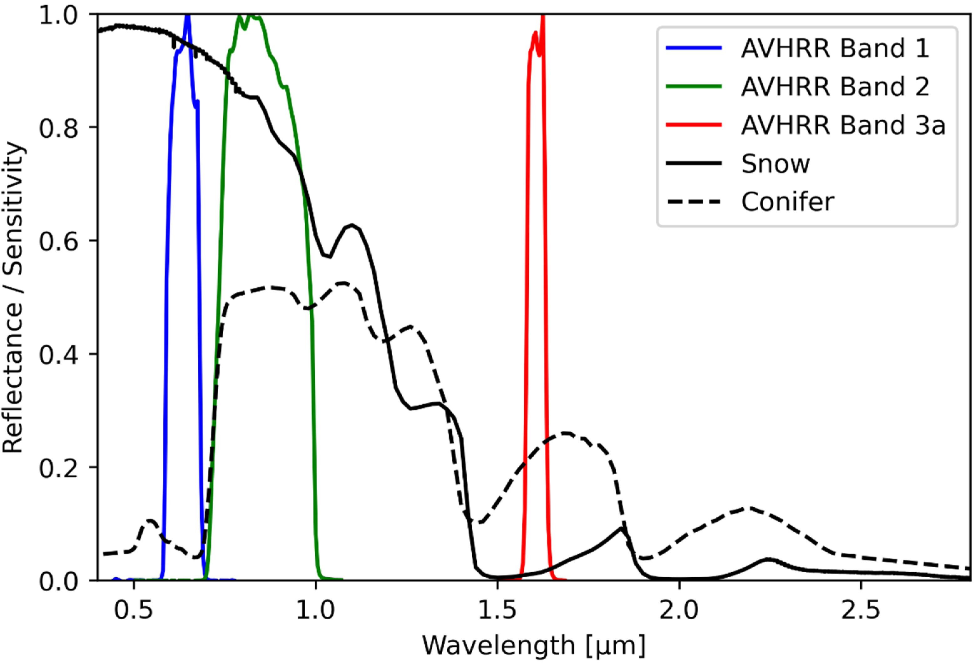
A very common method for detecting snow surfaces from the reflective part of the electromagnetic spectrum is to use snow’s unique spectral properties. Figure 1 shows the typical reflection properties of snow compared to vegetation (conifers in this example). In addition, the spectral response functions of the first three bands of the sensor AVHRR/3 (on NOAA-17) are shown.
In the reflection spectrum of snow, there is almost complete reflection in the visible spectral range (VIS: 0.38–0.78 µm). The reflection decreases rapidly in the near infrared (NIR: 0.78–1.4 µm), and in the short-wavelength infrared (SWIR: 1.4–3.0 µm), the radiation is almost completely absorbed. This extremely different reflection between VIS and SWIR is used in many methods for determining snow surfaces. Most methods for distinguishing between clouds and snow use a decision tree with fixed thresholds [8,9], which have to be adjusted individually depending on the region under consideration, such as the Alps [12,13]. The snow products from MODIS [3] are no longer based on fixed threshold values; instead, a normalized index is used that still maps the reflection gradient between VIS and SWIR well, even with lower reflections. Equation (1) shows the calculation of the Normalized Difference Snow Index (NDSI) [18] based on the AVHRR/3 spectral bands:
where is the atmospherically corrected reflectance in AVHRR Band 1 and the reflectance in Band 3a. The third generation of the AVHRR sensor has two options for using band 3: With variant 3a, the spectral range between 1.58 and 1.64 µm is recorded, but with variant 3b, however, the mid-wavelength infrared (MWIR) is between 3.55 and 3.93 µm. The two bands cannot be operated synchronously, so that there is either reflectance data or thermal data. This causes a problem in the NDSI calculation, since the reflectance data of band 3a is required (Equation (2)). This problem is solved by determining the reflective component of band 3b. The blackbody radiation of the brightness temperature determined from band 5 is used for this from the wavelength range of band 3b. This radiation is then subtracted from the recorded radiation of band 3b and normalized using the solar irradiance [8]:
where is the recorded radiance of band 3b (units: ), is the blackbody radiance at wavelength and temperature (i.e., brightness temperature of band 5), is the solar radiance corrected for the Earth–sun distance, and is the cosine of the sun zenith angle. The sensor-specific values of the wavenumbers and the solar radiance for the calculation of are taken from Trishchenko (2006) [19].
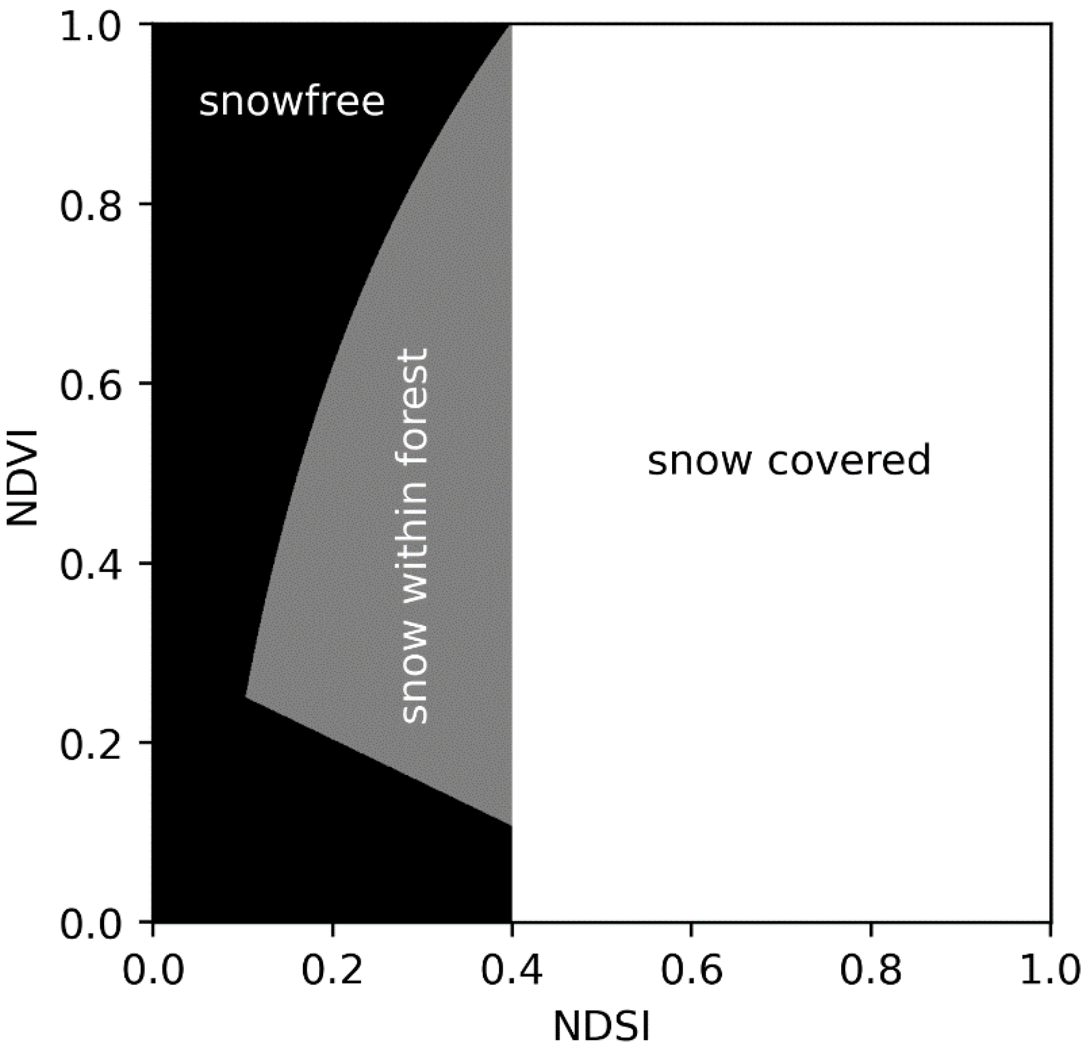
From the NDSI, the percentage of area covered with snow can also be determined. The NDSI threshold of 0.4 corresponds to a fractional snow cover of 50%, and all NDSI values above this threshold indicate more than 50% snow coverage [3,20,21]. Version 5 of the MODIS snow product used this threshold value to make a binary classification between snow (NDSI ≥ 0.4) and non-snow (NDSI < 0.4). Since version 6 (the latest version is 6.1), there is no longer a binary distinction, but all positive NDSI values are displayed in the “NDSI_snow_cover” layer, scaled between 0 and 100. This is due to the fact that a strict threshold value of 0.4 can lead to an underestimation of the detected snow surfaces in (especially coniferous) forests, which has been found by Klein et al. (1998) [22] by combining a snow reflectance model with a canopy reflectance model (GeoSAIL). Therefore, in addition to the NDSI, the Normalized Difference Vegetation Index (NDVI) is now also used to identify these snow areas in forests. The NDVI is calculated using Equation (3):
where is the atmospherically corrected reflectance in AVHRR Band 1 and the reflectance in Band 2. Based on NDSI and NDVI, depending on the NDVI value, a linear () and an exponential function () is used to create an area for the “snow within forest” class. The following functions (4a) to (4c) are based on Klein et al. (1998) [22]:
Based on the decision from Equation (4c), the area that forms the “snow within forest” class is shown in Figure 2. This additional area is also used for processing the AVHRR data.
2.2. Snow Cover—TIMELINE Level 2 Processor
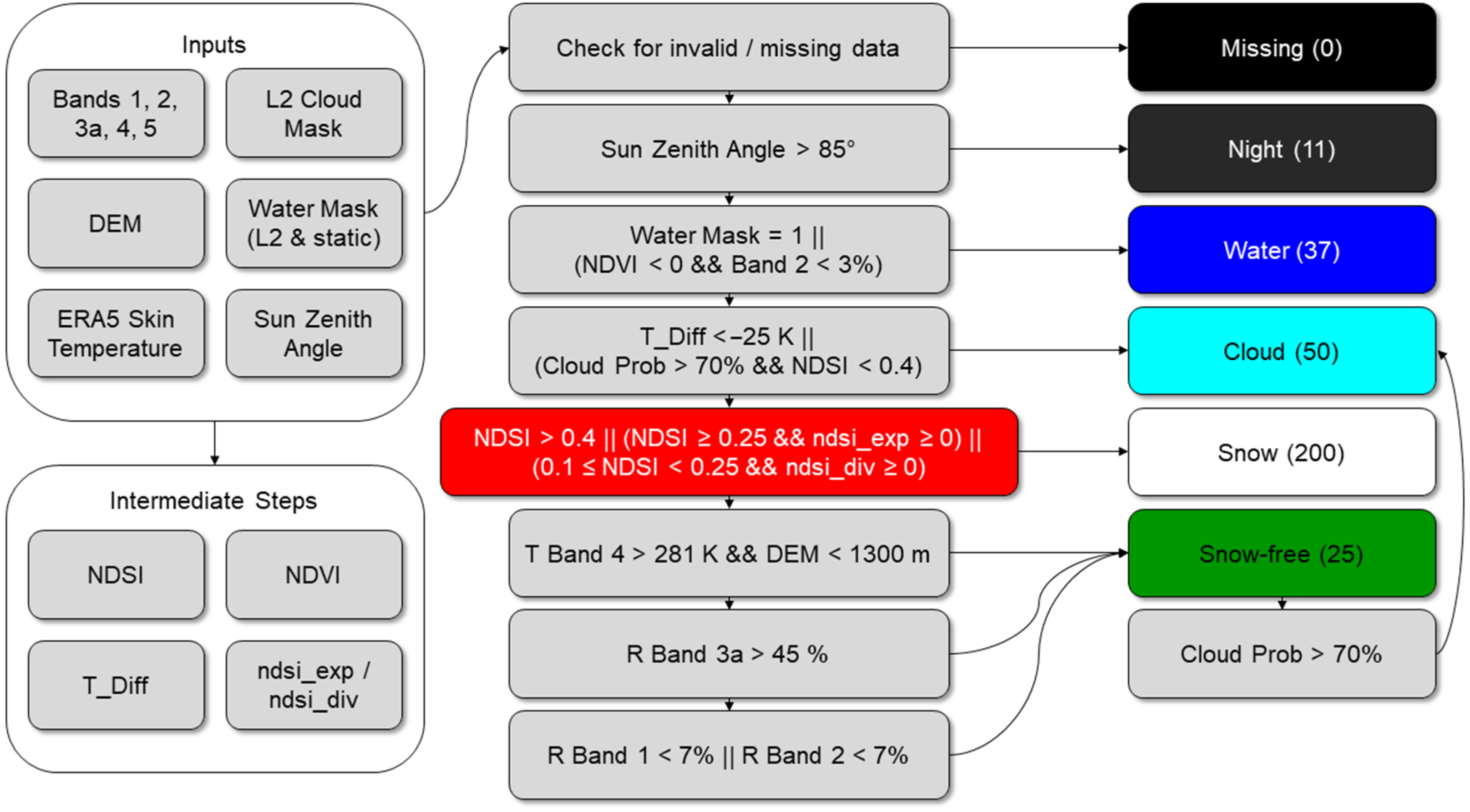
Based on the atmospherically corrected reflectance of the AVHRR Level 1b product, the Level 2 cloud mask [16], the Level 2 water mask [17], a static water mask, and ERA5 reanalysis data on the skin temperature [23] are required as input data. The reanalysis data are needed because distinguishing between clouds and snow using AVHRR is often challenging [24]. Therefore, the hourly skin temperature data are interpolated to the exact mean acquisition time of the scene, and the data set is converted into the swath projection of the orbit. The skin temperature is also linearly interpolated spatially in order to then create a difference raster between the brightness temperature of band 4 and the skin temperature. The cloud mask of APOLLO_NG [16] no longer specifies exact classes like APOLLO [9] but follows a probabilistic approach and provides probabilities for the occurrence of clouds.
This probabilistic cloud mask, the water masks (L2 product and static water mask), the calculated temperature difference, and the NDSI/NDVI classification explained in the previous chapter form the basis of the Level 2 snow processor. The steps are shown in Figure 3.
The first part of the processing is the masking of obvious cloud and water areas. This is performed with the Level 2 products mentioned, the static ocean/sea water mask, the NDVI, and the temperature difference. Areas with a solar zenith angle greater than 85° are classified as “night”. Then, according to Equation (4c), a provisional snow determination takes place. All land areas outside are classified as “snow free”. In the second part of the snow determination, additional probability thresholds are used, and snow pixels are re-classified if necessary. First, a temperature-height screen is applied: If the brightness temperature of band 4 is above 281 K and the terrain altitude is below 1300 m, the pixel is assigned to the “snow-free” class. The next screen concerns high SWIR reflectance: Pixels with more than 45% reflectance are determined as “snow free”. The last screen concerns the reflection in the visible range: If this is below 7% in band 1 or 2, the pixel is also declared as “snow-free”. For all remaining “snow-free” pixels, the cloud mask is used again, and all pixels with a cloud probability of over 70% are assigned to the “cloud” class. The cloud probability is an output layer of the Level 2 product cloud mask, which is computed with the probabilistic cloud processor APOLLO_NG [16]. The threshold value for the cloud probability of 70% was determined empirically, since clouds are best recognized here, and snow surfaces in this value range are usually not misclassified as clouds.
This division into classes forms the output layer “snow_mask” of the Level 2 product. In addition, the layer “raw_ndsi” is provided, which contains the raw NDSI values—the basis for snow determination. In addition, a “snow_quality_flag” layer is supplied, which hierarchically maps the quality of the classification in big-endian 8-bit coding (Table 1). The threshold values correspond to those of the MODIS snow product [3]. The daily aggregation of the Level 2 products in the Level 3 processor is based on this layer.
As can be seen from Table 1, the “snow_quality_flag” layer usually contains the same information as the “snow_mask” layer (Figure 3), but these are hierarchically structured and some differ: For example, if the brightness temperature of band 4 exceeds 281 K, the pixel is only reclassified to “snow free” if the elevation is below 1300 m—however, quality bit 5 is set in any case. If bit 4 is set, this does not cause a reclassification, but has a major impact on the detection of snow, since large sun zenith angles lead to poorer snow detection. Wang & Zender (2010) [25] have already determined quality losses from a sun zenith angle of more than 55°. However, since this threshold value would mean a large loss in surface area in winter, a sun zenith angle of over 70° was chosen for the MODIS snow product [3], from which point the quality flag is set. This is due to the unreliable albedo from 70°, which has been proven by radiative transfer and BRDF modelling [26,27,28,29]. The same is true for large satellite zenith angles, since at AVHRR/3, the pixel size increases from 1.08 km in nadir to 6.15 km at the edge (across-track) [30], and with it, the length of the path through the atmosphere. Since the cloud processor, for example, also has problems in these extreme peripheral areas of the scene (satellite zenith angle of ~68°), the flag “unfavorable illumination and/or observation geometry” was set for areas when the satellite zenith angle exceeds the empirically determined threshold of 65°.
2.3. Snow Cover—TIMELINE Level 3 Processor
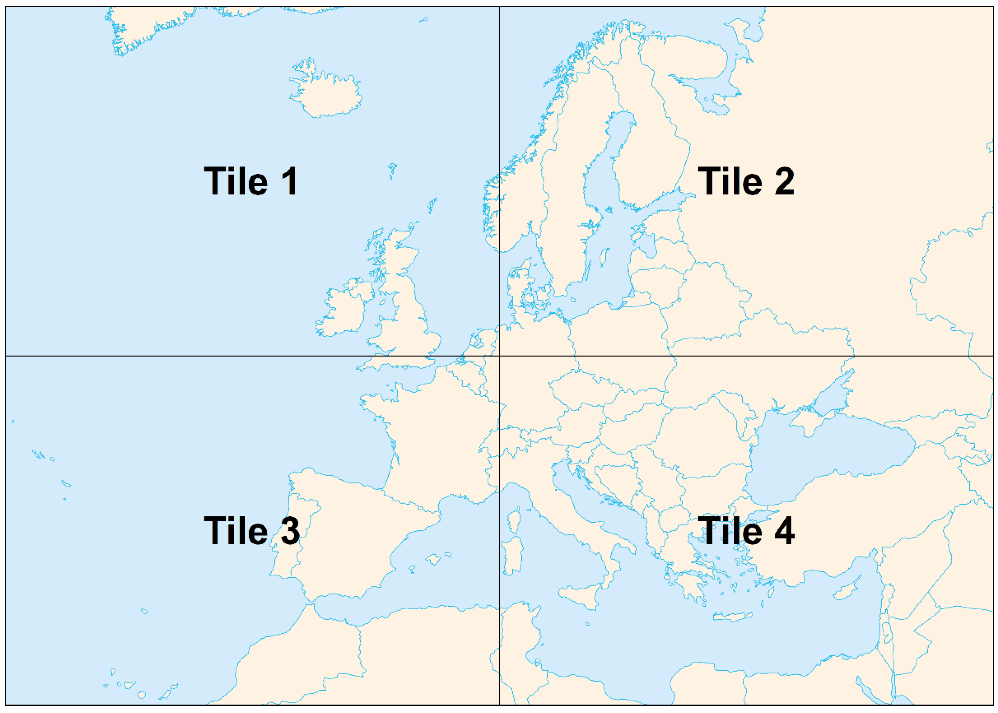
In contrast to the Level 2 products, the Level 3 products are available in geographical projection. ETRS89-extended/LAEA Europe (EPSG: 3035) was chosen as the target coordinate system, whereby the extent of the TIMELINE area (Europe, Middle East, and North Africa) was divided into four tiles (Figure 4).
The basis of all Level 3 products is the daily composite of all scenes available on that day. These are first projected into the respective tile. An output pixel size of 1000 m is selected, and “nearest neighbor” is selected as the resampling method. Only the “snow_mask” and “snow_quality_flag” layers are projected, with a no-data value of 0 or 255 being set. This gives the “snow_quality_flag” the highest value at this point, which is critical for further processing, since the processor is looking for the lowest value to fill the day composite. Two three-dimensional arrays are then created and filled with the two projected layers. The position with the minimum value is now searched for in the “snow_quality_flag” stack, and the final “snow_mask” is filled with the corresponding values of the “snow_mask” stack.
In addition to the daily composites, a 10-day product and a monthly product are also created. For this purpose, stacks are formed from 10 consecutive days or the whole month. From this, the minimum snow cover, the maximum snow cover, and the snow cover percentage of each pixel (without cloud cover) for the period under consideration are determined.
2.4. Validation with MODIS
The daily MODIS snow products [3] from Terra (MOD10A1, obtained from http://nsidc.org/data/MOD10A1, accessed on 19 December 2021) and Aqua (MYD10A1, obtained from http://nsidc.org/data/MYD10A1, accessed on 19 December 2021) in the latest version 6.1 are used to validate the snow mask. The entire TIMELINE area is covered by about 27 MODIS tiles (h16v01 to h21v05). These are downloaded, mosaicked, and converted into the target projection and pixel size for the period to be compared. A confusion matrix (Table 2) of the classes “snow” and “snow-free” is now created for all pixels that are cloud-free both in the AVHRR data and in the MODIS data.
The following indicators of classification accuracy can be determined from the confusion matrix: the true positive rate (), the true negative rate (), the positive predictive value (), the negative predictive value (), and the accuracy () [31]. The following Equations (5a)–(5e) show their determination from the confusion matrix:
3. Results
The Level 2 processor is applicable to all AVHRR Level 1B data of the TIMELINE Project, which is available at the German Aerospace Center (DLR) in the Local Area Coverage (LAC) with a 1 km spatial resolution. In the LAC mode, the recording time is limited to 10 min, but usually, the area is sufficient for the meridional expansion of the TIMELINE area (Figure 4). Although a channel in the SWIR (band 3a) is required for the NDSI calculation (Equation (1)), it can be calculated according to Equation (2) from the band 3b. We can therefore use the entire AVHRR archive that ranges from October 1981 to December 2018—this is a time series of 37 years. Since only a small part of the entire data set could be used for processor development, we chose 2009 as the test year. The winter of 2009 (and spring transition) showed all imaginable snow conditions in the examination area. For this period, MODIS data of the Terra and Aqua platforms are also available, which are used for validation.
3.1. Timeline Snow Cover—Level 2 and Level 3 Products
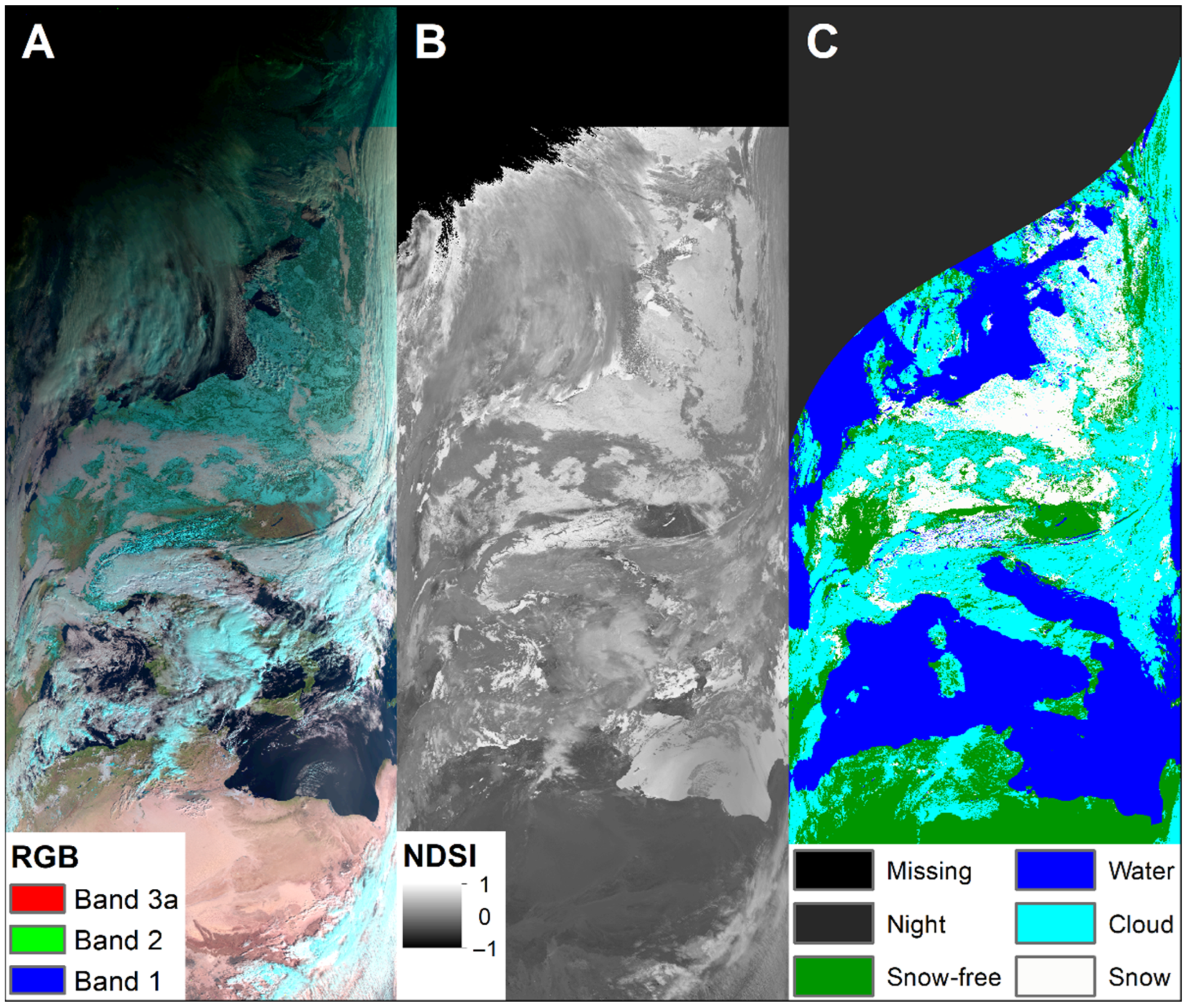
For testing, we focused on the months of January to April 2009. For the snow cover classifications, only day recordings can be used. However, since the number of Level 2 products created is very large (241 in January), Figure 5 shows an example of the processing steps from a scene on 8 January 2009.
Figure 5A shows snow-covered areas in the color cyan due to the RGB channel combination making clouds appear gray or white. In the upper section of Figure 5B (beginning of the recording), one can see a sharp transition due to the switching from band 3b (night mode) to band 3a (day mode). The NDSI image of Figure 5B also highlights the problem associated with this index for snow detection: In addition to snow, this index also takes a high value for water surfaces and some clouds [24]. The final classification result shows a satisfactory snow mask for this scene in Figure 5C. Clouds over seas were eliminated by the static water mask.
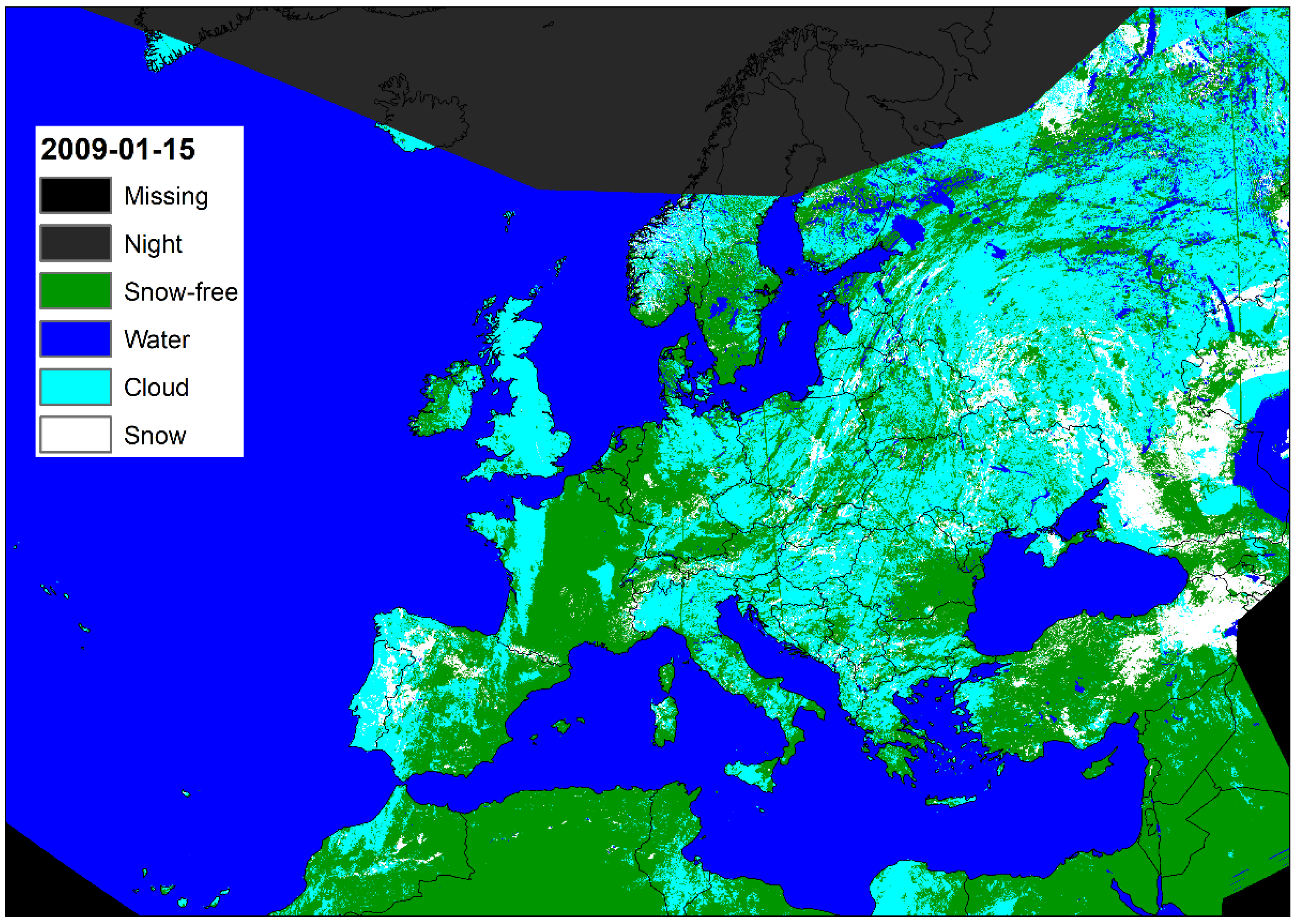
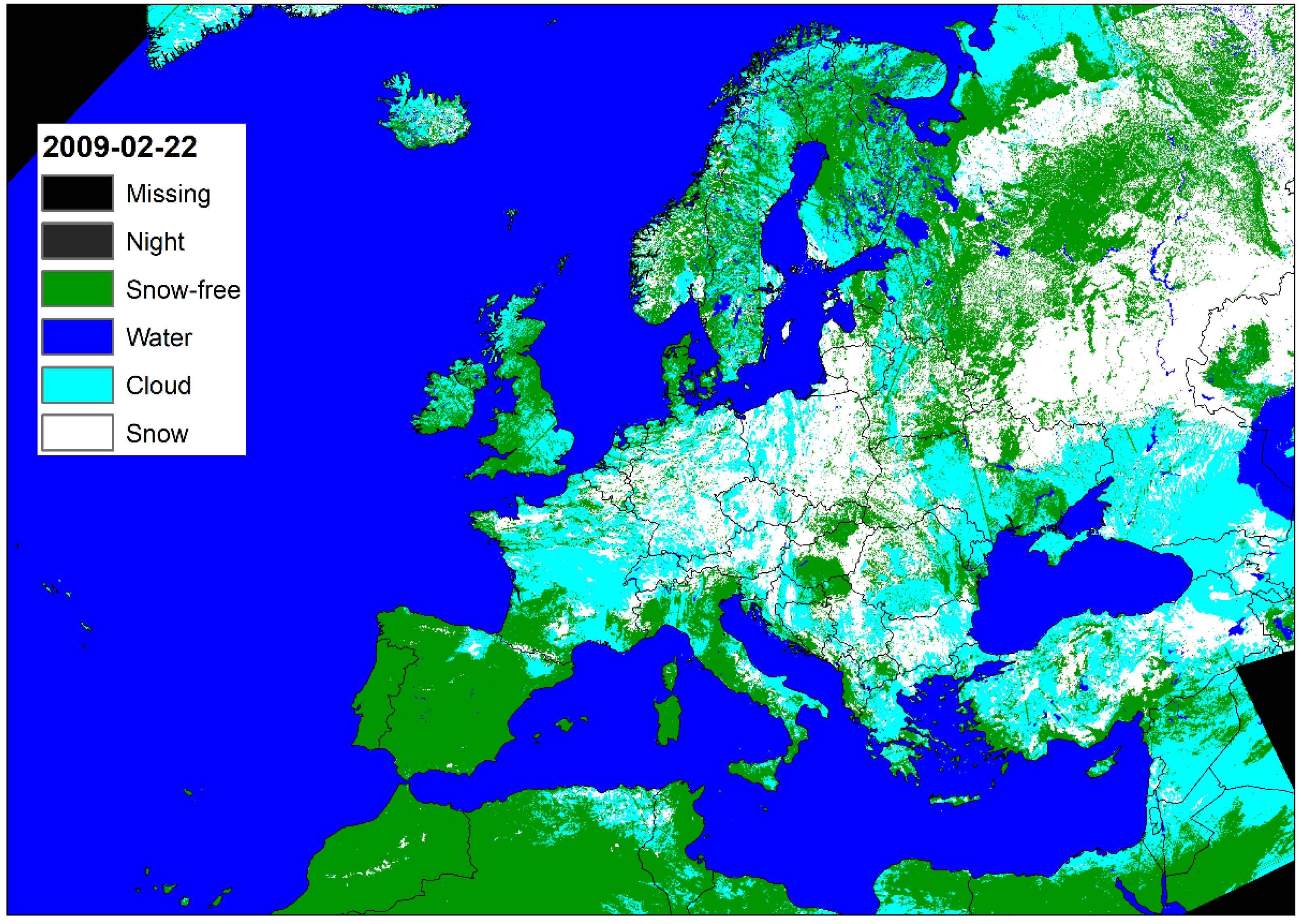
As examples for daily Level 3 products, 15 January 2009 (mid-winter) and 22 February 2009 (maximum snow coverage) were selected and are shown in Figure 6 and Figure 7.
Figure 6 and Figure 7 show linear artifacts in the overlap area of two level 2 products, which are due to insufficient cloud recognition on the image edge. The problem occurs with absolute satellite zenith angles larger than 65° and is labelled as a “bad satellite-viewing-geometry” in the quality layer (which also applies to a sun-zenith angle greater than 70°). It is also striking that wide parts of Fenno Scandia and northern Russia were classified as “snow-free”, which is unlikely at this season. In addition to the poor observation geometry, this is also due to a low reflection in the visible spectral range, whereby these areas are reclassified to “snow-free” despite a high NDSI. This leads to the accuracy analysis, which was carried out for these 4 months with MODIS snow data.
3.2. Validation Result
For validation, the daily MODIS snow products of Terra (MOD10A1) and Aqua (MYD10A1) had to be prepared first. For this purpose, the data of 27 MODIS tiles of both platforms were downloaded for the first 120 days of 2009. Then, the information of the layer “NDSI_snow_cover” was translated to the classes of the AVHRR snow product (Figure 3). The data of Terra and Aqua were then united to close possible data gaps through clouds [32]. Finally, the 27 tiles were mosaicked and transferred to the TIMELINE projection (Figure 4). The pixel size of 500 m was also scaled to 1 km, using a nearest neighbor resample algorithm. All preprocessing was performed with GDAL [33].
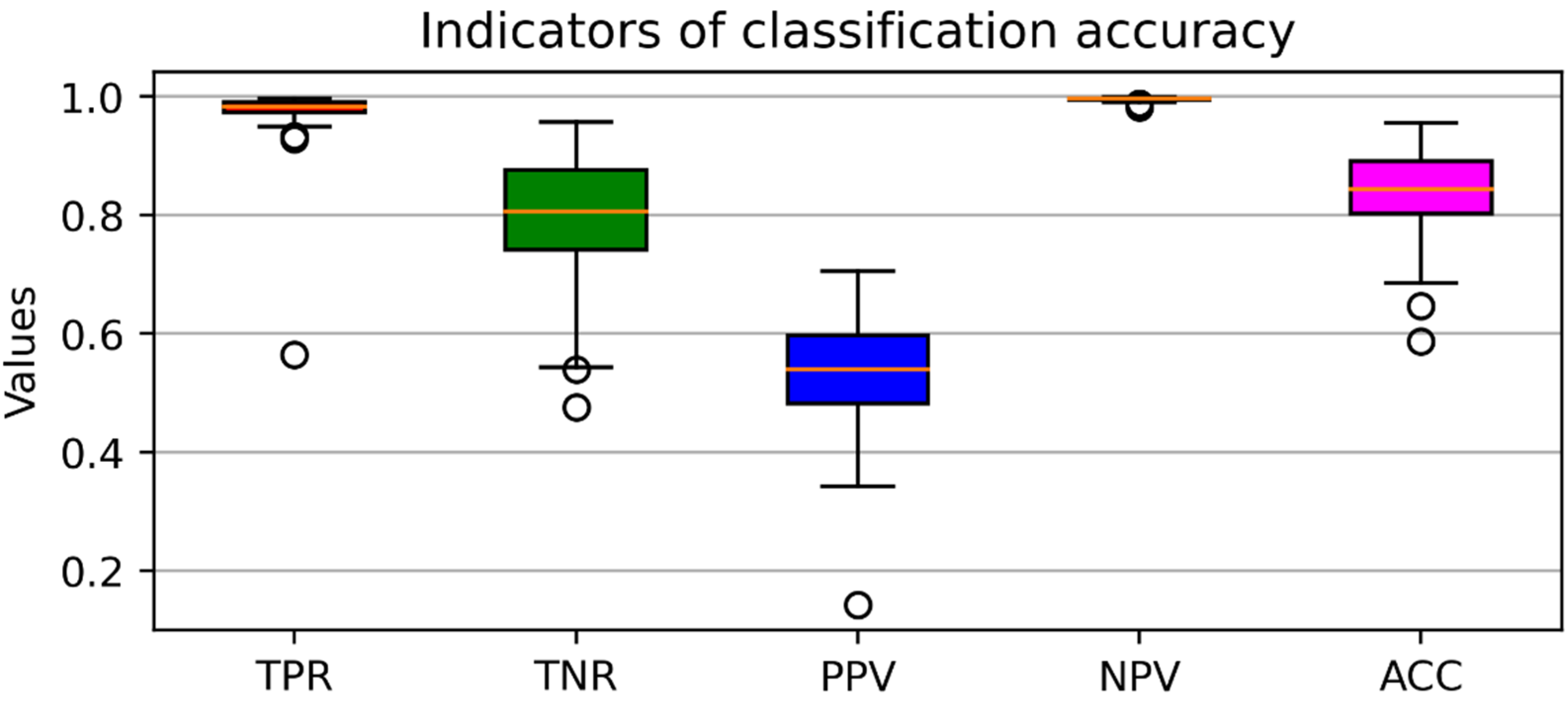
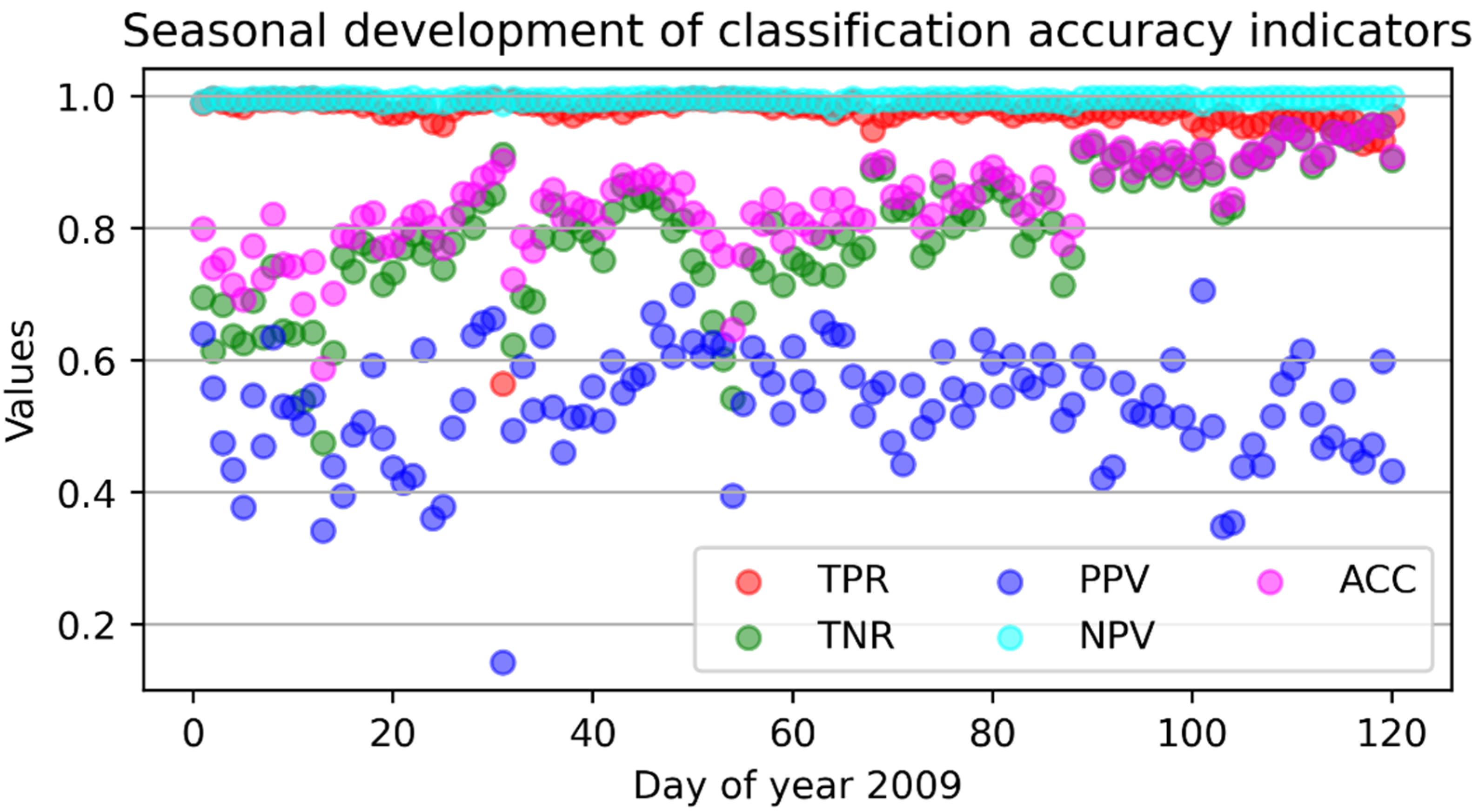
A confusion matrix (according to Table 2) was created for each day, which contains all pixels that have either the “snow” or “snow-free” classes in both the MODIS dataset and the AVHRR dataset. The “snow” class is considered a “true” value, and the “snow-free” class is considered a “false” value. Figure 8 shows the boxplots of the classification indicators of true positive rate (TPR), true negative rate (TNR), positive predictive value (PPV), negative predictive value (NPV), and accuracy (ACC) for all 120 days.
Figure 8 shows that the true positive rate (TPR) and negative predictive value (NPR) indicators are always close to 1 (100%). This is due to the fact that the proportion of snow-free areas in the entire TIMELINE area is always very high, even in winter–especially in northern Africa and the Middle East. Only the indicators true negative rate (TNR), positive predictive value (PPV) and accuracy (ACC) are suitable for a differentiated consideration of the results. Figure 9 therefore shows their seasonal development over the months of January to April.
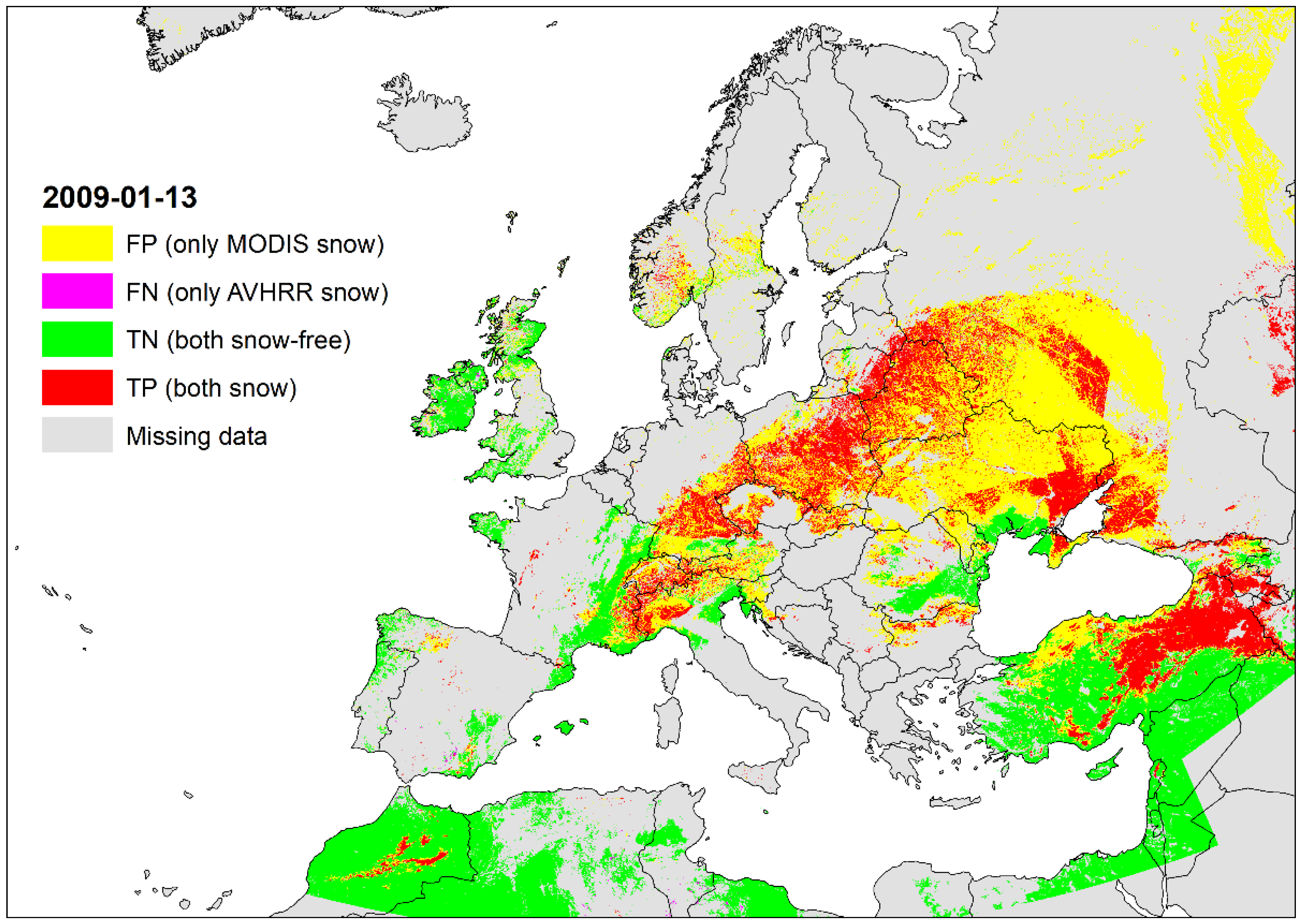
While no seasonality was found for the positive predictive value (PPV) indicator, it exists for true negative rate (TNR) and accuracy (ACC). There is an increase in both over time. On the one hand, this is due to the general decrease in snow cover, but on the other hand, it is also due to its better detection. So, it is worth having a closer look at the difference grids for the lowest and highest values of TNR, PPV, and ACC, respectively. The date 13 January 2009 stands out as a negative example, as this is when TNR, PPV, and ACC reach their lowest values. Figure 10 shows the misclassifications.
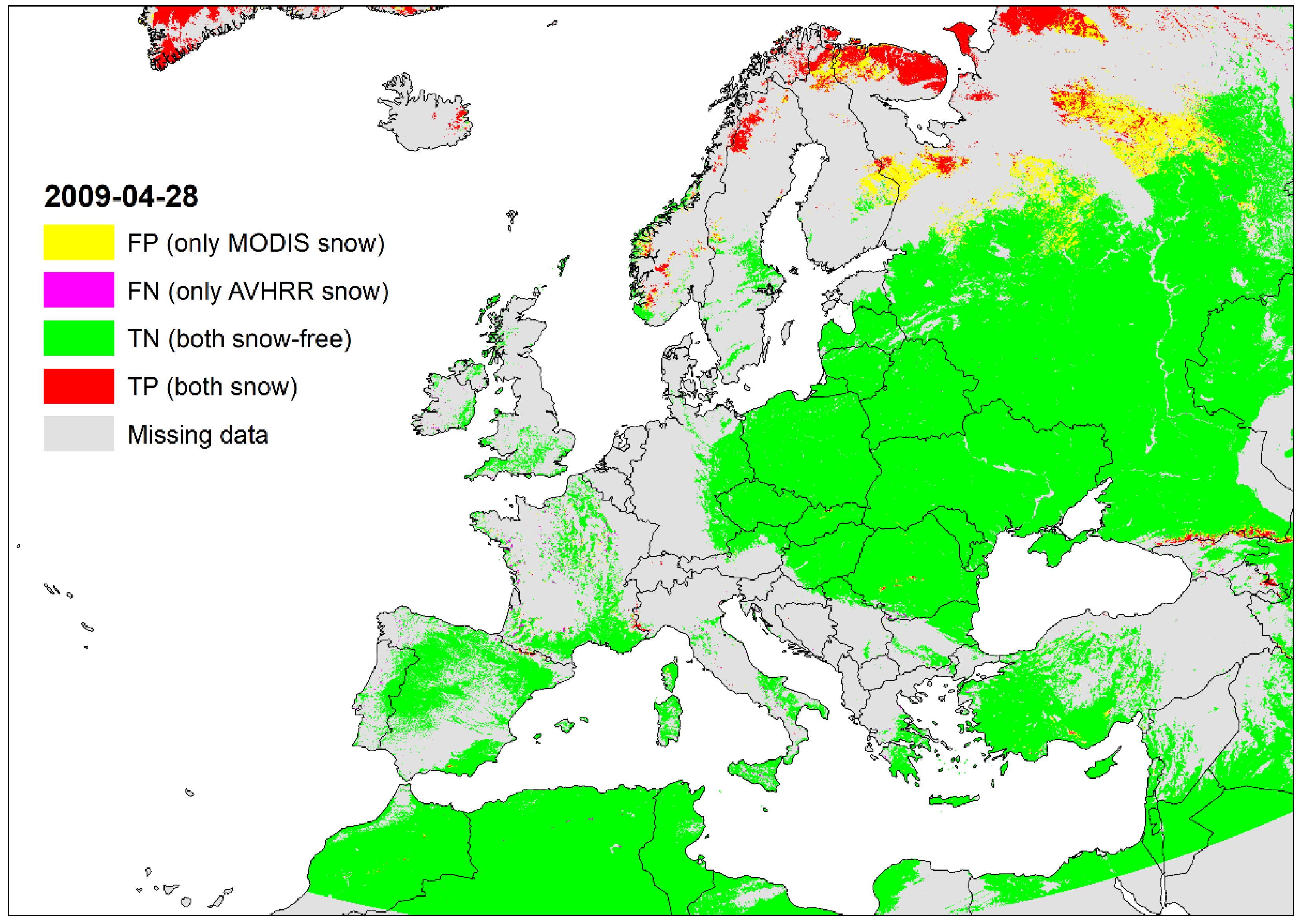
Figure 10 shows a large underestimation of snow cover by AVHRR in large parts of Eastern Europe (Ukraine, Belarus, Russia), as well as in the Alps. Due to the earlier point in time in the year (low sun altitude), this is again mainly due to the poor observation and illumination geometry. The later the time in the year, the better the illumination conditions and thus the results. Thus, on 28 April 2009, TNR and ACC show their highest (best) value (Figure 11).
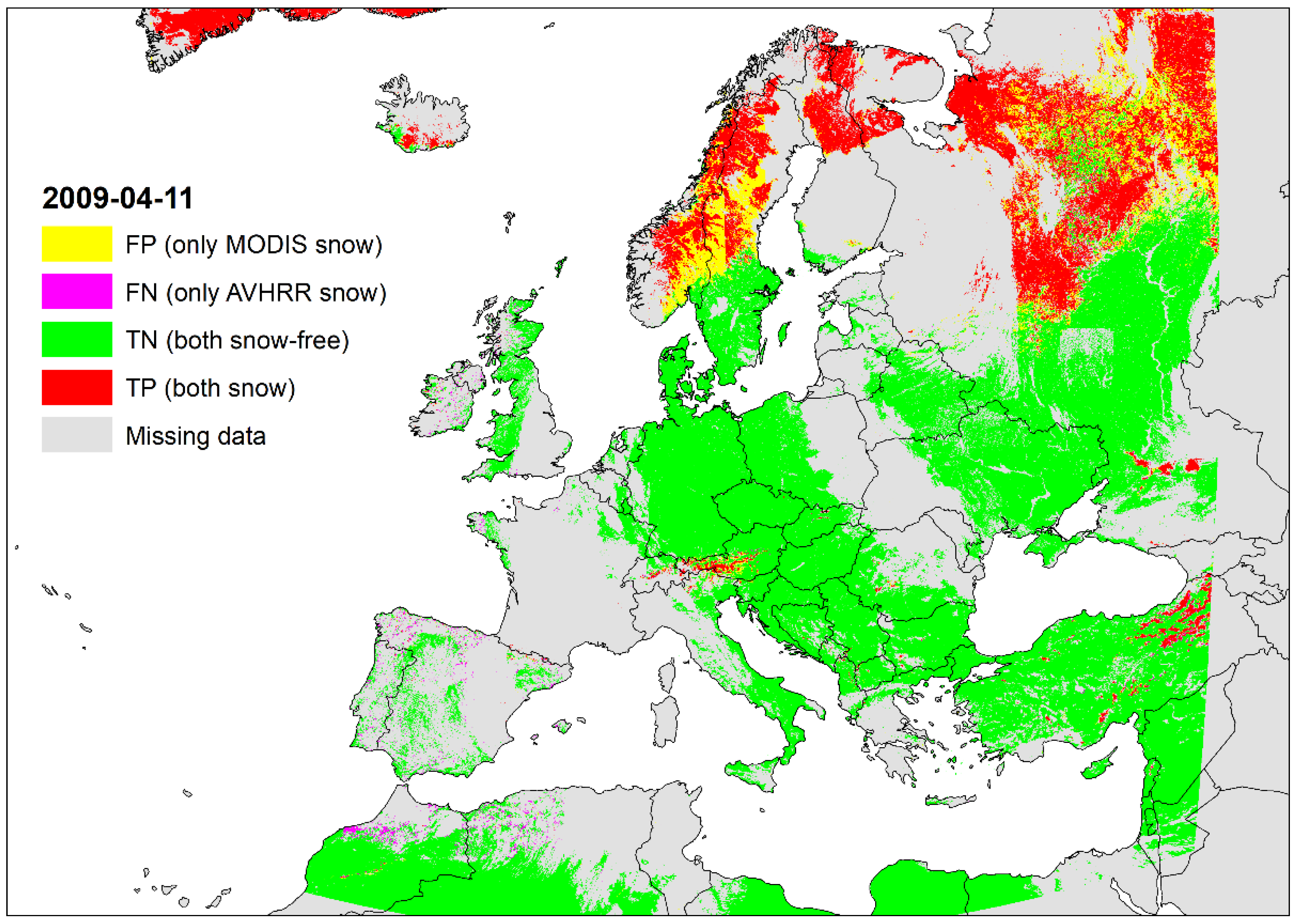
PPV also has its maximum in spring: on 11 April 2009. The snow cover is only underestimated in small areas of Scandinavia, the remaining areas are mapped well (Figure 12).
The examination of the difference grid shows that the improvement in the indicators is related to a better recognition of the snow surface and is independent of an increase in the “snow-free” area.
4. Discussion
Numerous methods have been developed to detect snow from AVHRR data. Snow cover is usually a by-product of cloud masking, as both classes have similar spectral properties [9,34,35,36]. The determination of the classes “snow” and “snow-free” is carried out either via a hierarchical classification [9], via probabilities (or scores) [8,13,37], or from multichannel thresholds combined with indices [38,39]. Although good results were achieved with hierarchical approaches [40], it turned out early on that they are not suitable for the present AVHRR data set. At least for the test period considered, we often received unusually low snow reflections in the VIS spectral range (far below the 80% given in Figure 1) for areas with a high sun zenith angle. This may be due to too much impact from the harmonization factors applied to the data set [4,41]. Since the SPARC algorithm [8,13], like APOLLO [9], also works with fixed reflection threshold values of the reflective bands, these were discarded, and an index-based algorithm was chosen with regard to comparability with MODIS [24]. The NDSI method makes snow detection independent of absolute reflection and BRDF effects over snow, which are known to have a strong influence on AVHRR [42]. Numerous evaluated threshold values [3,8,9,24] were used in the post-classification to eliminate particularly low reflections in the VIS, excessive brightness temperatures and too high reflections in the SWIR, which makes the result comparable with other methods for snow cover detection from AVHRR data.
The results of the validation against the MODIS snow product show that the classification quality increases with increasing sun elevation (decreasing sun zenith angle). Sun zenith angles of more than 70° are generally not well suited for determining snow from optical remote sensing data [25]. Due to the mentioned underestimation of the reflection in the VIS of the Level 1b products due to atmospheric correction and harmonization, snow-covered areas are reclassified as “snow-free”. In addition, there are already inaccuracies in the Level 2 products used, so that cloud detection in the area of the scene edges (satellite zenith angle > 65°) can fail or snow areas can be recognized as clouds. The larger area at the edge of the scene and the longer path through the atmosphere also lead to a loss in radiation, particularly in the short-wave spectrum. There, the VIS-reflections can fall below the threshold of 7% and be reassigned to the “snow-free” class. This can be seen in Figure 12 in the area of Sweden and Norway, where both a large sun zenith angle and peripheral areas of a scene (high satellite zenith angle) lead to incorrect classification.
This leads to the question of how we can solve the identified problems? A drastic possibility would be that all “inaccurate” Level 2 scene excerpts—which do not meet the quality standards mentioned in Table 1—are excluded from the Level 3 product generation. However, this would mean an immense loss of information, since large areas of the snow-covered northern hemisphere would not be mapped. Eliminating the VIS threshold would improve snow detection, but this decision should be made using a larger data set (several years, platforms, and sensor generations). The Level 3 processor is currently being implemented in the TIMELINE processing environment [4], and then the entire data set will be processed with it. This will give us more information on how good the results are for the different platforms and sensor versions. High-resolution Landsat data will then be used for validation, which will enable subpixel analysis [43,44].
When the entire data series has been processed, a daily cloud-free AVHRR product covering a unique time series of almost 40 years is created from the daily data analogous to DLR’s Global SnowPack [45]. This enables the observation of hydrological processes at the catchment area level [15,46,47] and, for example, the investigation of snow changes in mountains [11,12], which was previously not possible for this long period of time. The data can also be used with other environmental data for hydrological modeling in order to investigate the occurrence of extreme situations in climatologically relevant periods [48,49].
5. Conclusions
In this manuscript, the first results of the thematic snow cover processor of the TIMELINE project were presented. In TIMELINE, a data set from almost 40 years of AVHRR data is reprocessed according to up-to-date processing methods. One of the thematic products is snow cover, the largest and most ephemeral part of the cryosphere. The results for the test period presented here (the first 4 months of 2009) show good agreement between AVHRR snow cover and the daily MODIS product used as a reference. In general, however, AVHRR underestimates snow under poor lighting conditions (high sun zenith angle). The processor is now applied to the entire dataset to re-validate the results and adjust them if necessary. The time series created in this way will offer a variety of options for investigating the change in snow cover for a wide variety of questions.
Author Contributions
Conceptualization, S.R. and A.J.D.; methodology, S.R. and A.J.D.; software, S.R.; validation, S.R.; formal analysis, S.R. and A.J.D.; investigation, S.R. and A.J.D.; resources, S.R.; data curation, A.J.D.; writing—original draft preparation, S.R.; writing—review and editing, S.R. and A.J.D.; visualization, S.R.; supervision, A.J.D.; project administration, A.J.D.; funding acquisition, A.J.D. All authors have read and agreed to the published version of the manuscript.
Funding
This research received no external funding.
Institutional Review Board Statement
Not applicable.
Informed Consent Statement
Not applicable.
Data Availability Statement
The TIMELINE Level 2 data used will be made available via the EOC GeoService portal (https://geoservice.dlr.de/web/) in the near future, as will the snow cover data generated (Level 2 and Level 3). The ECMWF Reanalysis v5 (ERA5) data are available from https://www.ecmwf.int/en/forecasts/dataset/ecmwf-reanalysis-v5 (accessed on 1 June 2021).
Acknowledgments
This work was funded by the German Aerospace Center (DLR). We thank DLR headquarters for the funding of the TIMELINE project. The authors would like to thank the editors and three anonymous reviewers who, with their suggestions and comments, significantly improved the quality of the manuscript.
Conflicts of Interest
The authors declare no conflict of interests.
References
- Intergovernmental Oceanographic Commission (IOC). The Global Observing System for Climate; GCOS-No. 200; World Meteorological Organization (WMO): Geneva, Switzerland, 2016. [Google Scholar]
- Dietz, A.J.; Kuenzer, C.; Gessner, U.; Dech, S. Remote Sensing of Snow—A Review of Available Methods. Int. J. Remote Sens. 2012, 33, 4094–4134. [Google Scholar] [CrossRef]
- Hall, D.K.; Riggs, G.A.; Salomonson, V.V.; DiGirolamo, N.E.; Bayr, K.J. MODIS Snow-Cover Products. Remote Sens. Environ. 2002, 83, 181–194. [Google Scholar] [CrossRef] [Green Version]
- Dech, S.; Holzwarth, S.; Asam, S.; Andresen, T.; Bachmann, M.; Boettcher, M.; Dietz, A.; Eisfelder, C.; Frey, C.; Gesell, G.; et al. Potential and Challenges of Harmonizing 40 Years of AVHRR Data: The TIMELINE Experience. Remote Sens. 2021, 13, 3618. [Google Scholar] [CrossRef]
- Harrison, A.R.; Lucas, R.M. Multi-Spectral Classification of Snow Using NOAA AVHRR Imagery. Int. J. Remote Sens. 1989, 10, 907–916. [Google Scholar] [CrossRef]
- Lindsay, R.W.; Rothrock, D.A. Arctic Sea Ice Albedo from AVHRR. J. Climate 1994, 7, 1737–1749. [Google Scholar] [CrossRef] [Green Version]
- Dozier, J.; Schneider, S.R.; McGinnis, D.F. Effect of Grain Size and Snowpack Water Equivalence on Visible and Near-Infrared Satellite Observations of Snow. Water Resour. Res. 1981, 17, 1213–1221. [Google Scholar] [CrossRef] [Green Version]
- Khlopenkov, K.V.; Trishchenko, A.P. SPARC: New Cloud, Snow, and Cloud Shadow Detection Scheme for Historical 1-Km AVHHR Data over Canada. J. Atmos. Ocean. Technol. 2007, 24, 322–343. [Google Scholar] [CrossRef]
- Gesell, G. An Algorithm for Snow and Ice Detection Using AVHRR Data An Extension to the APOLLO Software Package. Int. J. Remote Sens. 1989, 10, 897–905. [Google Scholar] [CrossRef]
- Zhu, J.; Shi, J. An Algorithm for Subpixel Snow Mapping: Extraction of a Fractional Snow-Covered Area Based on Ten-Day Composited AVHRR\/2 Data of the Qinghai-Tibet Plateau. IEEE Geosci. Remote Sens. Mag. 2018, 6, 86–98. [Google Scholar] [CrossRef]
- Akyürek, Z.; Şorman, A.Ü. Monitoring Snow-Covered Areas Using NOAA-AVHRR Data in the Eastern Part of Turkey. Hydrol. Sci. J. 2002, 47, 243–252. [Google Scholar] [CrossRef] [Green Version]
- Hüsler, F.; Jonas, T.; Riffler, M.; Musial, J.P.; Wunderle, S. A Satellite-Based Snow Cover Climatology (1985–2011) for the European Alps Derived from AVHRR Data. Cryosphere 2014, 8, 73–90. [Google Scholar] [CrossRef] [Green Version]
- Hüsler, F.; Jonas, T.; Wunderle, S.; Albrecht, S. Validation of a Modified Snow Cover Retrieval Algorithm from Historical 1-Km AVHRR Data over the European Alps. Remote Sens. Environ. 2012, 121, 497–515. [Google Scholar] [CrossRef]
- Foppa, N.; Wunderle, S.; Oesch, D.; Kuchen, F. Operational Sub-Pixel Snow Mapping over the Alps with NOAA AVHRR Data. Ann. Glaciol. 2004, 38, 245–252. [Google Scholar] [CrossRef] [Green Version]
- Peters, J.; Bolch, T.; Gafurov, A.; Prechtel, N. Snow Cover Distribution in the Aksu Catchment (Central Tien Shan) 1986–2013 Based on AVHRR and MODIS Data. IEEE J. Sel. Top. Appl. Earth Obs. Remote Sens. 2015, 8, 5361–5375. [Google Scholar] [CrossRef]
- Klüser, L.; Killius, N.; Gesell, G. APOLLO_NG—A Probabilistic Interpretation of the APOLLO Legacy for AVHRR Heritage Channels. Atmos. Meas. Tech. 2015, 8, 4155–4170. [Google Scholar] [CrossRef] [Green Version]
- Dietz, A.; Klein, I.; Gessner, U.; Frey, C.; Kuenzer, C.; Dech, S. Detection of Water Bodies from AVHRR Data—A TIMELINE Thematic Processor. Remote Sens. 2017, 9, 57. [Google Scholar] [CrossRef] [Green Version]
- Hall, D.K.; Riggs, G.A. Normalized-Difference Snow Index (NDSI). In Encyclopedia of Snow, Ice and Glaciers; Singh, V.P., Singh, P., Haritashya, U.K., Eds.; Encyclopedia of Earth Sciences Series; Springer: Dordrecht, The Netherlands, 2011; ISBN 978-90-481-2641-5. [Google Scholar]
- Trishchenko, A.P. Solar Irradiance and Effective Brightness Temperature for SWIR Channels of AVHRR/NOAA and GOES Imagers. J. Atmos. Ocean. Technol. 2006, 23, 198–210. [Google Scholar] [CrossRef]
- Salomonson, V.V.; Appel, I. Estimating Fractional Snow Cover from MODIS Using the Normalized Difference Snow Index. Remote Sens. Environ. 2004, 89, 351–360. [Google Scholar] [CrossRef]
- Salomonson, V.V.; Appel, I. Development of the Aqua MODIS NDSI Fractional Snow Cover Algorithm and Validation Results. IEEE Trans. Geosci. Remote Sens. 2006, 44, 1747–1756. [Google Scholar] [CrossRef]
- Klein, A.G.; Hall, D.K.; Riggs, G.A. Improving Snow Cover Mapping in Forests through the Use of a Canopy Reflectance Model. Hydrol. Process. 1998, 12, 1723–1744. [Google Scholar] [CrossRef]
- Copernicus Climate Change Service. ERA5-Land Hourly Data from 2001 to Present; European Commission: Brussels, Belgium, 2019. [Google Scholar]
- Villaescusa-Nadal, J.L.; Vermote, E.; Franch, B.; Santamaria-Artigas, A.E.; Roger, J.-C.; Skakun, S. MODIS-Based AVHRR Cloud and Snow Separation Algorithm. IEEE Trans. Geosci. Remote Sens. 2022, 60, 5400513. [Google Scholar] [CrossRef]
- Wang, X.; Zender, C.S. MODIS Snow Albedo Bias at High Solar Zenith Angles Relative to Theory and to In Situ Observations in Greenland. Remote Sens. Environ. 2010, 114, 563–575. [Google Scholar] [CrossRef] [Green Version]
- Lucht, W. Expected Retrieval Accuracies of Bidirectional Reflectance and Albedo from EOS-MODIS and MISR Angular Sampling. J. Geophys. Res. 1998, 103, 8763–8778. [Google Scholar] [CrossRef] [Green Version]
- Schaaf, C.B.; Gao, F.; Strahler, A.H.; Lucht, W.; Li, X.; Tsang, T.; Strugnell, N.C.; Zhang, X.; Jin, Y.; Muller, J.-P.; et al. First Operational BRDF, Albedo Nadir Reflectance Products from MODIS. Remote Sens. Environ. 2002, 83, 135–148. [Google Scholar] [CrossRef] [Green Version]
- Wang, Z. The Solar Zenith Angle Dependence of Desert Albedo. Geophys. Res. Lett. 2005, 32, L05403. [Google Scholar] [CrossRef]
- Liu, J.; Schaaf, C.; Strahler, A.; Jiao, Z.; Shuai, Y.; Zhang, Q.; Roman, M.; Augustine, J.A.; Dutton, E.G. Validation of Moderate Resolution Imaging Spectroradiometer (MODIS) Albedo Retrieval Algorithm: Dependence of Albedo on Solar Zenith Angle: VALIDATION OF MODIS ALBEDO ON SZN. J. Geophys. Res. 2009, 114. [Google Scholar] [CrossRef]
- Klaes, K.D. The EUMETSAT Polar System. In Comprehensive Remote Sensing; Elsevier: Amsterdam, The Netherlands, 2018; pp. 192–219. ISBN 978-0-12-803221-3. [Google Scholar]
- Fawcett, T. An Introduction to ROC Analysis. Pattern Recognit. Lett. 2006, 27, 861–874. [Google Scholar] [CrossRef]
- Hall, D.K.; Riggs, G.A.; Foster, J.L.; Kumar, S.V. Development and Evaluation of a Cloud-Gap-Filled MODIS Daily Snow-Cover Product. Remote Sens. Environ. 2010, 114, 496–503. [Google Scholar] [CrossRef] [Green Version]
- Rouault, E.; Warmerdam, F.; Schwehr, K.; Kiselev, A.; Butler, H.; Łoskot, M. GDAL; Zenodo: Genève, Switzerland, 2022. [Google Scholar]
- Saunders, R.W.; Kriebel, K.T. An Improved Method for Detecting Clear Sky and Cloudy Radiances from AVHRR Data. Int. J. Remote Sens. 1988, 9, 123–150. [Google Scholar] [CrossRef]
- Allen, R.C.; Durkee, P.A.; Wash, C.H. Snow/Cloud Discrimination with Multispectral Satellite Measurements. J. Appl. Meteorol. 1990, 29, 994–1004. [Google Scholar] [CrossRef] [Green Version]
- Derrien, M.; Farki, B.; Harang, L.; LeGléau, H.; Noyalet, A.; Pochic, D.; Sairouni, A. Automatic Cloud Detection Applied to NOAA-11 /AVHRR Imagery. Remote Sens. Environ. 1993, 46, 246–267. [Google Scholar] [CrossRef]
- Musial, J.P.; Hüsler, F.; Sütterlin, M.; Neuhaus, C.; Wunderle, S. Probabilistic Approach to Cloud and Snow Detection on Advanced Very High Resolution Radiometer (AVHRR) Imagery. Atmos. Meas. Tech. 2014, 7, 799–822. [Google Scholar] [CrossRef] [Green Version]
- Voigt, S.; Koch, M.; Baumgartner, M.F. Operational Monitoring of Snow Cover in the Swiss Alps Using Real-Time NOAA-AVHRR Data. In Proceedings of the IEEE 1999 International Geoscience and Remote Sensing Symposium, IGARSS’99 (Cat. No.99CH36293). Hamburg, Germany, 28 June–1 July; IEEE: Hamburg, Germany, 1999; Volume 2, pp. 1077–1079. [Google Scholar]
- Voigt, S.; Koch, M.; Baumgartner, M. A Multichannel Threshold Technique for NOAA AVHRR Data to Monitor the Extent of Snow Cover in the Swiss Alps. In Interactions between the Cryosphere, Climate and Greenhouse Gases; IAHS-AISH Publication: Wallingford, UK, 1999; pp. 35–43. [Google Scholar]
- Dietz, A.; Conrad, C.; Kuenzer, C.; Gesell, G.; Dech, S. Identifying Changing Snow Cover Characteristics in Central Asia between 1986 and 2014 from Remote Sensing Data. Remote Sens. 2014, 6, 12752–12775. [Google Scholar] [CrossRef] [Green Version]
- Steven, M.D.; Malthus, T.J.; Baret, F.; Xu, H.; Chopping, M.J. Intercalibration of Vegetation Indices from Different Sensor Systems. Remote Sens. Environ. 2003, 88, 412–422. [Google Scholar] [CrossRef]
- Zhonghai, J.; Simpson, J.J. Bidirectional Anisotropic Reflectance of Snow and Sea Ice in AVHRR Channel 1 and 2 Spectral Regions. I. Theoretical Analysis. IEEE Trans. Geosci. Remote Sens. 1999, 37, 543–554. [Google Scholar] [CrossRef]
- Hao, X.; Huang, G.; Che, T.; Ji, W.; Sun, X.; Zhao, Q.; Zhao, H.; Wang, J.; Li, H.; Yang, Q. The NIEER AVHRR Snow Cover Extent Product over China—A Long-Term Daily Snow Record for Regional Climate Research. Earth Syst. Sci. Data 2021, 13, 4711–4726. [Google Scholar] [CrossRef]
- Huang, X.; Liang, T.; Zhang, X.; Guo, Z. Validation of MODIS Snow Cover Products Using Landsat and Ground Measurements during the 2001–2005 Snow Seasons over Northern Xinjiang, China. Int. J. Remote Sens. 2011, 32, 133–152. [Google Scholar] [CrossRef]
- Dietz, A.J.; Kuenzer, C.; Dech, S. Global SnowPack: A New Set of Snow Cover Parameters for Studying Status and Dynamics of the Planetary Snow Cover Extent. Remote Sens. Lett. 2015, 6, 844–853. [Google Scholar] [CrossRef]
- Notarnicola, C.; Duguay, M.; Moelg, N.; Schellenberger, T.; Tetzlaff, A.; Monsorno, R.; Costa, A.; Steurer, C.; Zebisch, M. Snow Cover Maps from MODIS Images at 250 m Resolution, Part 1: Algorithm Description. Remote Sens. 2013, 5, 110–126. [Google Scholar] [CrossRef] [Green Version]
- Matikainen, L.; Kuittinen, R.; Vepsäläinen, J. Estimating Drainage Area-Based Snow-Cover Percentages from NOAA AVHRR Images. Int. J. Remote Sens. 2002, 23, 2971–2988. [Google Scholar] [CrossRef]
- Rößler, S.; Witt, M.S.; Ikonen, J.; Brown, I.A.; Dietz, A.J. Remote Sensing of Snow Cover Variability and Its Influence on the Runoff of Sápmi’s Rivers. Geosciences 2021, 11, 130. [Google Scholar] [CrossRef]
- Jain, S.K.; Goswami, A.; Saraf, A.K. Accuracy Assessment of MODIS, NOAA and IRS Data in Snow Cover Mapping under Himalayan Conditions. Int. J. Remote Sens. 2008, 29, 5863–5878. [Google Scholar] [CrossRef]
Figure 1.
Reflective properties of snow compared to vegetation. The spectral response functions (sensitivity) for the AVHRR bands 1 to 3a are shown, with channels 1 and 2 being available for all AVHRR sensors, but channel 3a only for the third generation (AVHRR/3) and on MetOP-A and -B.
Figure 1.
Reflective properties of snow compared to vegetation. The spectral response functions (sensitivity) for the AVHRR bands 1 to 3a are shown, with channels 1 and 2 being available for all AVHRR sensors, but channel 3a only for the third generation (AVHRR/3) and on MetOP-A and -B.

Figure 2.
NDSI thresholds for detecting snow. The area was expanded based on the NDVI values for the “snow in the forest” class.
Figure 2.
NDSI thresholds for detecting snow. The area was expanded based on the NDVI values for the “snow in the forest” class.

Figure 3.
Flowchart of the TIMELINE Snow Mask Processor. The central NDSI-based snow recognition is highlighted with red color.
Figure 3.
Flowchart of the TIMELINE Snow Mask Processor. The central NDSI-based snow recognition is highlighted with red color.

Figure 4.
Tiling scheme of the TIMELINE area in ETRS89-extended/LAEA Europe projection.

Figure 5.
Example of a Level 2 snow cover product in satellite swath projection from 8 January 2009 (recording time 09:15:00–09:26:26 UTC); Platform NOAA-17; Sensor AVHRR/3. (A) RGB composite from the Level 1b bands 3a, 2, 1; (B) from band 1 and band 3a calculated NDSI (gradient of black, −1, towards white, +1); (C) snowmask created according to the sheme presented in Figure 3.

Figure 6.
Example of a daily Level 3 product for 15 January 2009 (mid-winter).

Figure 7.
Example of a Daily Level 3 product for 22 February 2009 (maximum snow coverage).

Figure 8.
Boxplots showing the variance of classification accuracy indicators during the first 120 days of the test year 2009.
Figure 8.
Boxplots showing the variance of classification accuracy indicators during the first 120 days of the test year 2009.

Figure 9.
The development of classification accuracy indicators over the months January to April 2009 (i.e., the first 120 days of the year).
Figure 9.
The development of classification accuracy indicators over the months January to April 2009 (i.e., the first 120 days of the year).

Figure 10.
Daily composite of the classification accuracy for 13 January 2009–the date with the fewest matches between MODIS and AVHRR (TNR: 47.5%, PPV: 34.25%, and ACC: 58.67%).
Figure 10.
Daily composite of the classification accuracy for 13 January 2009–the date with the fewest matches between MODIS and AVHRR (TNR: 47.5%, PPV: 34.25%, and ACC: 58.67%).

Figure 11.
Daily composite of the classification accuracy for 28 April 2009—the date with the best matches between MODIS and AVHRR in terms of TNR (95.67%) and ACC (95.58%).
Figure 11.
Daily composite of the classification accuracy for 28 April 2009—the date with the best matches between MODIS and AVHRR in terms of TNR (95.67%) and ACC (95.58%).

Figure 12.
Daily composite of the classification accuracy for 11 April 2009—the date with the best matches between MODIS and AVHRR in terms of PPV (70.54%).
Figure 12.
Daily composite of the classification accuracy for 11 April 2009—the date with the best matches between MODIS and AVHRR in terms of PPV (70.54%).


Table 1.
Description of the bits in the layer “snow_quality_flag”.
| Bit | Value | Description |
|---|---|---|
| 1 | 128 | Missing data or night (solar zenith angle > 85°) |
| 2 | 64 | Pixel covered with clouds |
| 3 | 32 | Pixel classified as water |
| 4 | 16 | Unfavorable illumination and/or observation geometry (sun zenith angle > 70°, satellite zenith angle > 65°) |
| 5 | 8 | Brightness temperature of Band 4 too high (>281 K) |
| 6 | 4 | SWIR reflectance too high (>25%–reclassified to “snow free” if >45%) |
| 7 | 2 | VIS Reflectance too low (<7% in Band 1 or 2) |
| 8 | 1 | Pixels classified as “snow free” |
Table 2.
Confusion matrix to determine classification accuracy with MODIS data.
| MODIS | |||
|---|---|---|---|
| Snow | Snow-Free | ||
| AVHRR | Snow | TP (true positive) | FP (false positive) |
| Snow-free | FN (false negative) | TN (true negative) | |
Publisher’s Note: MDPI stays neutral with regard to jurisdictional claims in published maps and institutional affiliations. |
© 2022 by the authors. Licensee MDPI, Basel, Switzerland. This article is an open access article distributed under the terms and conditions of the Creative Commons Attribution (CC BY) license (https://creativecommons.org/licenses/by/4.0/).
Share and Cite
MDPI and ACS Style
Rößler, S.; Dietz, A.J. Detection of Snow Cover from Historical and Recent AVHHR Data—A Thematic TIMELINE Processor. Geomatics 2022, 2, 144-160. https://0-doi-org.brum.beds.ac.uk/10.3390/geomatics2010009
AMA Style
Rößler S, Dietz AJ. Detection of Snow Cover from Historical and Recent AVHHR Data—A Thematic TIMELINE Processor. Geomatics. 2022; 2(1):144-160. https://0-doi-org.brum.beds.ac.uk/10.3390/geomatics2010009
Chicago/Turabian StyleRößler, Sebastian, and Andreas J. Dietz. 2022. "Detection of Snow Cover from Historical and Recent AVHHR Data—A Thematic TIMELINE Processor" Geomatics 2, no. 1: 144-160. https://0-doi-org.brum.beds.ac.uk/10.3390/geomatics2010009