
Density, Enthalpy of Vaporization and Local Structure of Neat N-Alkane Liquids
by
 , , , and
Gerrick E. Lindberg
1,2,* ,
,
Joseph L. Baker
3,
Jennifer Hanley
4,5,
William M. Grundy
4,5 and
Caitlin King
1,2 1
Center for Materials Interfaces in Research and Applications, Department of Applied Physics and Materials Science, Northern Arizona University, Flagstaff, AZ 86011, USA
2
Department of Chemistry, Northern Arizona University, Flagstaff, AZ 86011, USA
3
Department of Chemistry, The College of New Jersey, Ewing, NJ 08628, USA
4
Lowell Observatory, Flagstaff, AZ 86001, USA
5
Department of Astronomy and Planetary Science, Northern Arizona University, Flagstaff, AZ 86011, USA
*
Author to whom correspondence should be addressed.
Liquids 2021, 1(1), 47-59; https://0-doi-org.brum.beds.ac.uk/10.3390/liquids1010004
Submission received: 30 May 2021
/
Revised: 13 July 2021
/
Accepted: 3 August 2021
/
Published: 6 August 2021
Abstract
:The properties of alkanes are consequential for understanding many chemical processes in nature and industry. We use molecular dynamics simulations with the Amber force field GAFF2 to examine the structure of pure liquids at each respective normal boiling point, spanning the 15 n-alkanes from methane to pentadecane. The densities predicted from the simulations are found to agree well with reported experimental values, with an average deviation of 1.9%. The enthalpies of vaporization have an average absolute deviation from experiment of 10.4%. Radial distribution functions show that short alkanes have distinct local structures that are found to converge with each other with increasing chain length. This provides a unique perspective on trends in the n-alkane series and will be useful for interpreting similarities and differences in the n-alkane series as well as the breakdown of ideal solution behavior in mixtures of these molecules.
1. Introduction
Alkanes are common in nature and are frequently used in various applications in chemical industries [1]. While it’s not feasible to list all scientific and technological areas that involve alkanes, a few examples can provide a useful perspective on how the study of alkanes at the molecular scale can have a significant impact across many sectors of science and the economy. In particular, we wish to highlight that alkanes frequently occur in heterogeneous systems, composed of many molecules and phases at a wide range of pressures and temperatures. Petroleum is composed overwhelmingly of hydrocarbons and often a significant portion are alkanes [2]. The process of refining and cracking crude oil entails an examination of alkane behavior in numerous environments and conditions [2]. Methane and other small hydrocarbons occur in Earth’s atmosphere and are consequential greenhouse gases [3,4]. Alkanes are much more reactive than CO2, however, so they have far shorter lifetimes in the atmosphere [3]. Their reactivity is important for their use in synthetic organic chemistry as well as linked to their hypothesized roles in the natural formation of complex organic molecules particularly in abiotic conditions. Venturing beyond Earth, these molecules are common in many extraterrestrial environments, comprising a significant portion of some planetary surfaces and atmospheres [5,6,7]. Many of these examples feature complex mixtures of molecules, so the use and evaluation of robust, transferable force fields for such systems is an opportunity to look at more realistic systems without the need for time consuming parameterization or slower simulation protocols. Additionally, they often serve as the first molecules introduced in organic chemistry courses. Beyond pedagogical convenience, they are also important models of the driving forces underlying the behavior of hydrophobic molecules, particularly as they relate to biological questions, like protein folding [8,9,10], protein-protein interactions [8,9,10], lipid structure and dynamics [11,12,13], and other topics. As such, their behavior provides context for the properties of hydrophobic molecules and is relevant for understanding a diverse set of natural and technological processes.
Despite their apparent simplicity and ubiquitous prevalence, alkanes remain a frequent topic of inquiry. Here we focus on normal alkanes, n-alkanes, which are hydrocarbon molecules with a linear chain of fully saturated carbon atoms. These molecules have general molecular formulas of the form CH3-(Cn-2H2n-4)-CH3 or more compactly CnH2n+2, where n is the number of carbon atoms in the molecule. The structure of n-alkanes was the topic of some of the first X-ray diffraction studies of aliphatic molecules in liquids [14]. These studies helped establish and inform our understanding of molecular structure, like bond lengths, angles, and dihedral angles. Many of the small n-alkane liquids have received significant attention. For example, Habenschuss et al. used X-ray diffraction to study the structure of liquid methane [15]. Despite methane itself appearing spherically symmetric in X-ray experiments, intermolecular structural correlations revealed distributions indicative of tetrahedral molecular symmetry [15]. Similar studies have been reported for ethane [16], propane [17], n-butane [18], n-pentane [19], and so on. A common thread through these studies is that n-alkanes have increasing molecular flexibility with length and present richly complicated intermolecular structures. These studies go beyond understanding just the structure of the molecule itself but reveal correlations between multiple molecules. This permits the elucidation of solvation structure when n-alkanes are used as the solvent. Additionally, it has permitted the exploration of processes like solvation and desolvation of solutes, wetting and dewetting of surfaces, nucleation, etc. Indeed, in this work, we are particularly interested in the intermolecular structure of alkane liquids as a path to understand the thermodynamics of these systems. This liquid structure provides a new perspective on n-alkanes as solvents, but also on features specific to liquid phase behavior.
There have been numerous molecular simulation studies of n-alkanes, both examining their specific properties and as model systems to evaluate force fields and other aspects of simulation protocols [9,12,20,21,22,23,24,25,26]. Density is frequently presented, because it is straightforward to determine, a holistic measure of force field performance, and typically unambiguously comparable with experimental results. Many force fields, developed with different philosophies and parameterized using many different strategies, have been shown to accurately reproduce experimental densities for these systems [9]. Many force fields are specifically tuned to reproduce the density at some state point for the system of interest, but general force fields are constructed to on average provide adequate description of molecular interactions so that thermodynamic and dynamic behavior is suitably reproduced. As such, density serves as an important test of the performance of a molecular model.
In this work, we perform molecular dynamics simulations to examine the density and radial distribution functions of pure n-alkane liquids, from methane to pentadecane, to understand similarities and differences in the local structure of these liquids. We are specifically interested in the variation of liquid structure as the number of carbon atoms in the alkane increases. We find that there are several signatures of convergence with respect to chain length, depending on the property examined. This set of molecules is known to have trends in many thermodynamic properties with increasing n, which are often used to understand how intermolecular forces and molecular size affect thermodynamic properties (indeed they are often presented in general and organic chemistry to help new students understand relationships between molecule structure and emergent properties). Further, while this study does not directly consider mixtures, the convergence of properties for pure n-alkanes can be used to anticipate the onset, or conversely the breakdown, of ideal solution principles in mixtures.
2. Materials and Methods
2.1. Simulation Methods
2.1.1. Liquid Simulation Details and Protocol
The starting structures for each n-alkane were imported from the WebMO chemical structure database [27]. WebMO was used to set up and execute Gaussian calculations using Gaussian version 16 [28]. The molecular structure was optimized and then the electrostatic potential was calculated using Hartree–Fock theory with a 6-31G* basis. The atomic partial charges for each n-alkane were then assigned using the RESP method [29] as implemented in the AmberTools program Antechamber. AmberTools and Amber version 20 were used for all parameterization and simulation steps in this study, unless otherwise stated [30]. The second generation general Amber force field (GAFF2) was used to describe the van der Waals, bond, angle, and dihedral interaction terms in all molecules [31]. The starting parameter files for simulations were constructed using the AmberTools program tLEaP [30]. Starting configurations containing 1000 molecules of an n-alkane were prepared using the Packmol utility to randomly place the molecules in a cubic simulation cell [32]. The starting box size was selected to obtain starting densities of about 0.1 g/mL. This size is chosen to balance the desire to reduce so-called ‘bad contacts’ (arrangements of molecules in relatively high energy configurations resulting in large forces that are difficult to relax to equilibrium) in the starting configuration with the practical limitation of obtaining a configuration quickly.
Each system was first relaxed using 10,000 minimization steps, where the initial 10 steps use the steepest descent algorithm and the remaining use the conjugate gradient method. Second, to obtain the approximate liquid density, each n-alkane system was equilibrated in the NPT (isobaric, isothermal) ensemble at the experimental normal (1 bar) boiling point for the molecule for approximately 10 ns. The boiling points for each n-alkane at 1 bar are listed in Table 1. All simulations use a time step of 1 fs. The temperature is maintained with the Langevin thermostat with a collision frequency of 5 ps−1. In all isobaric simulations, the pressure was controlled with the isotropic Berendsen barostat using a relaxation time of 1 ps. Third, each system was annealed for 20 ns in the NVT (isochoric, isothermal) ensemble 200 K above the normal boiling point of the molecule. This is intended to remove spurious effects that may have resulted from the randomly generated starting configuration. Fourth, the system was equilibrated for 20 ns in the NPT ensemble at the experimental normal boiling point of the molecule using the same parameters as step 2. An additional simulation was initiated from the end of this 20 ns simulation 10 K below the boiling point for each alkane for the numerical determination of the entropy of binding (discussed more below). Fifth and last, production for each system at the boiling point and 10 K below was performed by simulating for 100 ns in the NPT ensemble. These production simulations are analyzed for the properties reported here.
2.1.2. Gas Simulation Details and Protocol
We also performed gas phase simulations for the calculation of the enthalpy of vaporization, . We generally followed the method described by Wang and Tingjun (in Wang and Tingjun this is called protocol 4 or “P4”) [24]. For each alkane, a single molecule was placed in a 100 Å box and simulated NVT at the experimental boiling point for 1.1 ns. The last 1 ns was used for the calculation of required average quantities. Otherwise, the simulation parameters were the same as previously described for liquids.
2.2. Analysis of Simulations
2.2.1. Density
The mass density is included in the standard output from Amber molecular dynamics simulations performed in the NPT ensemble. The values reported here are calculated by averaging the production simulations.
2.2.2. Enthalpy of Vaporization ()
The enthalpy of vaporization, , is the enthalpy difference between the gas and liquid at a given state point. That is
where the subscripts indicate the given phase. In this work, we followed a protocol to approximate Equation (1) developed by Wang and Tingjun [24]. More information and discussion can be found in their original paper [24], but briefly they showed that can be predicted from molecular dynamics with the expression
where is the average potential energy of the gas phase simulation, is the average potential energy of the liquid simulation per molecule, is the gas constant, is the difference in average temperatures from the simulations in each phase (that is, ), and is the number of atoms in the molecule. Wang and Tingjun found that can be better estimated from an ensemble of minimized energies obtained from gas phase dynamics, but in this work we used the energies directly from the dynamics.
2.2.3. Radial Distribution Functions, Free Energy of Binding, and Entropy of Binding
The radial distribution functions are calculated using the AmberTools simulation analysis tool cpptraj [34]. We consider two types of radial distribution functions: those between all carbon atoms in a system and those between a specific carbon in the chain and all other carbon atoms. Subsequent thermodynamic analysis uses the radial distribution function calculated between all carbon atoms in the system. The free energy of binding, ΔGbind, is determined from the maximum value in the radial distribution function as
where kB is Boltzmann’s constant, T is the temperature, and RDFmax is the maximum value in the radial distribution function for that molecule. In this context, the term binding is used to describe the non-specific intermolecular association of pairs of molecules. The total average binding free energy is calculated as n ΔGbind, where n is the number of carbon atoms in the molecule and ΔGbind is obtained from Equation (3). The entropy of binding is estimated numerically from the relationship
ΔGbind = −kBT ln(RDFmax),
This derivative is evaluated numerically for each molecule with two simulations performed at the boiling point and 10 K below the boiling point.
3. Results
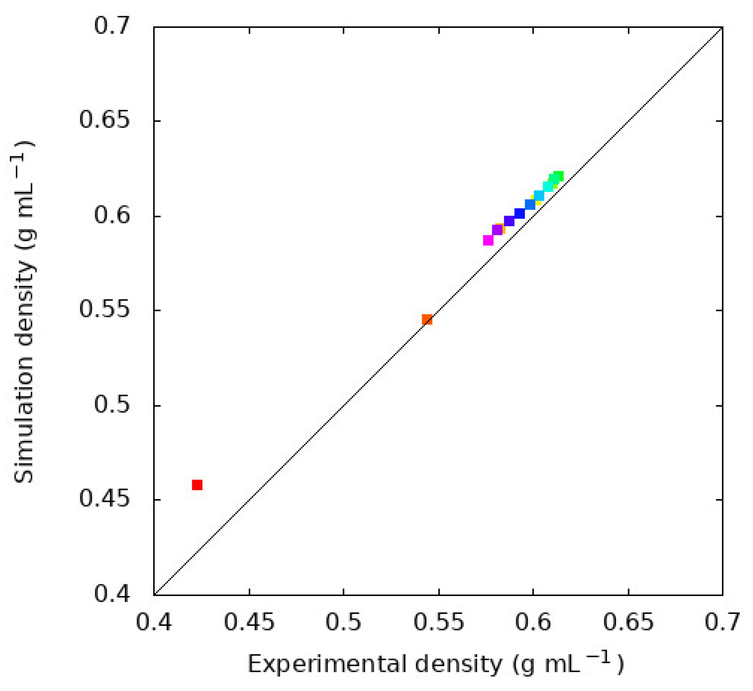
The density and are often viewed as important evaluations of the quality of a molecular model, especially the non-bonded terms. Figure 1 shows the density of each n-alkane at the normal (1 bar) boiling point. Figure 2 compares the simulations reported here with experimental densities via a parity plot. Table 2 compares from our simulations compared with experimental values.
Structure of the liquids is evaluated using radial distribution functions. In Figure 3, we examine the radial distribution functions between all carbon atoms within a system. Further, in Figure 4, we examine the local structure around specific carbon atoms. These compare the structure around the terminal carbon with all other carbon atoms (Figure 4a), around the second carbon from the end (Figure 4b), around the third carbon from the end (Figure 4c), and so on. Both ends of each alkane are symmetric, so neither are shown. Only the longest alkane, pentadecane, has an interior carbon that is eight bonds from a terminal carbon, so it is the only molecule in Figure 4h.
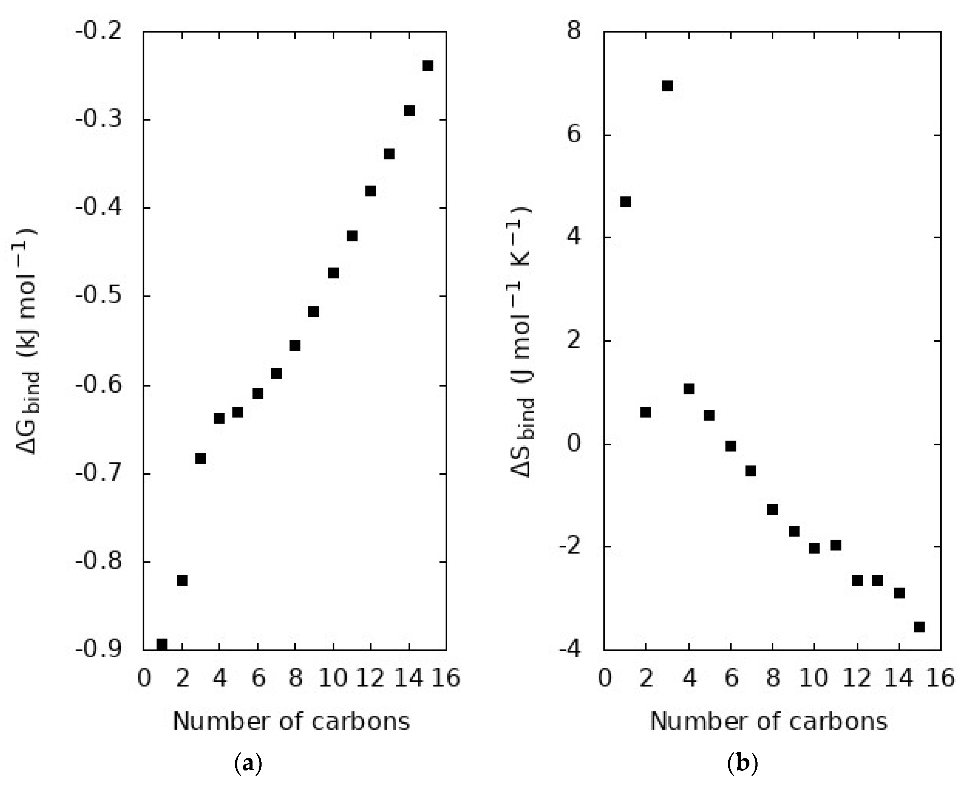
We examined the free energy and entropy of binding in Figure 5. The free energy of binding is calculated from the maximum value in the radial distribution functions shown in Figure 3. The entropy of binding is determined from the free energy of binding in Figure 5a as well as the analysis of another simulation 10 K below the boiling point of the molecule. Figure 5a is the average free energy binding a carbon from a molecule in the liquid, so we also examine n ΔGbind in Figure 6, as a measure of the total average binding free energy holding each molecule in solution.
4. Discussion
4.1. Density, , and Evaluation of the GAFF2 Force Field for N-Alkanes
Figure 2 shows that the GAFF2 force field with RESP charges faithfully reproduces n-alkane liquid densities at the normal boiling point. The density emerges as a complex result of the interaction potential for a given molecule, so this is often regarded as an important measure of the quality of a force field. We find that all simulations overestimate the density with an average overestimation of 1.9% for all 15 molecules. The largest deviation between simulation and experiment is observed for methane, with the simulations overestimating the density by 8%. The GAFF2, and its first-generation predecessor GAFF, force field are developed with the goal of simulating organic molecules in biological contexts, so the deviation of methane can be rationalized. Methane is the shortest alkane and while it does appear in natural biological processes it is distinct from the relatively longer, greasy sp3 carbon chains where carbon more often appears in biologically relevant molecules. This is reflected in the training set of molecules used to parameterize GAFF, which includes many sp3 hybridized carbons, but not methane [31]. Indeed, we find that, without methane, the average deviation between experiment and simulation drops to 1.4%.
Table 2 shows as predicted by our simulations compared with experimental values from the NIST database. The average absolute deviation between simulation and experimental value is 10.4%. The errors are not uniformly distributed, however, with progressive underestimation of the increase in for longer alkanes. For short hydrocarbons, the simulations overestimate and for longer alkanes the enthalpy increases less steeply than experiment. This presents a more complex picture of the fidelity of GAFF2 to reproduce alkane properties than the density. Like the density, shorter alkanes are seen to deviate most from experiment. There are entire studies dedicated to optimizing protocols for the calculation of , so there remains some opportunity to refine the protocol. For example, Wang and Tingjun showed that the result is sensitive to thermostat and many aspects of how configurations are collected and prepared [24].
GAFF2 is the second-generation general Amber force field which is designed to model organic molecules, especially in biological environments [30]. It evolved in functional form and parameterization strategy from the OPLS force fields [20], which focuses on functional group parameterization. This means that the interaction parameters used here are not tuned specifically to these n-alkanes, but rather to all hydrocarbons with similar atom types. This grants credibility to the use of GAFF2 for systems and conditions like those considered in this work, which admittedly deviate far from the biological systems that motivated the original development of GAFF2.
When Jorgensen et al. introduced the OPLS/AA force field, they included ethane, propane, and butane in the training set of more than 50 organic molecules [20]. In their evaluation of the force field, they found that densities deviated by 2% for all molecules, or 1% for just the three n-alkanes tested, and deviated by 3% for all molecules or 1% for the alkanes. OPLS/AA differs from many other force fields because it specifically targeted parameterization for the liquid phase, which resulted in better performance. In a broader assessment of force fields spanning more types of molecules, GAFF was found to have an average error of 4.43% and 16.43% from experiments for density and , respectively [24]. Caleman et al. developed a protocol for testing force fields that included density and with many small molecules and applied it to GAFF, OPLS/AA, and CGenFF [36]. They found percent deviations in density of 4%, 2%, and 2% and in of 17%, 11%, and 7%, for each force field, respectively. Our results are closer on average to the experiment for many of these force fields, but n-alkanes are less of a challenge than the diverse collection of molecules included in many of these studies.
4.2. Average Structure in N-Alkane Liquids
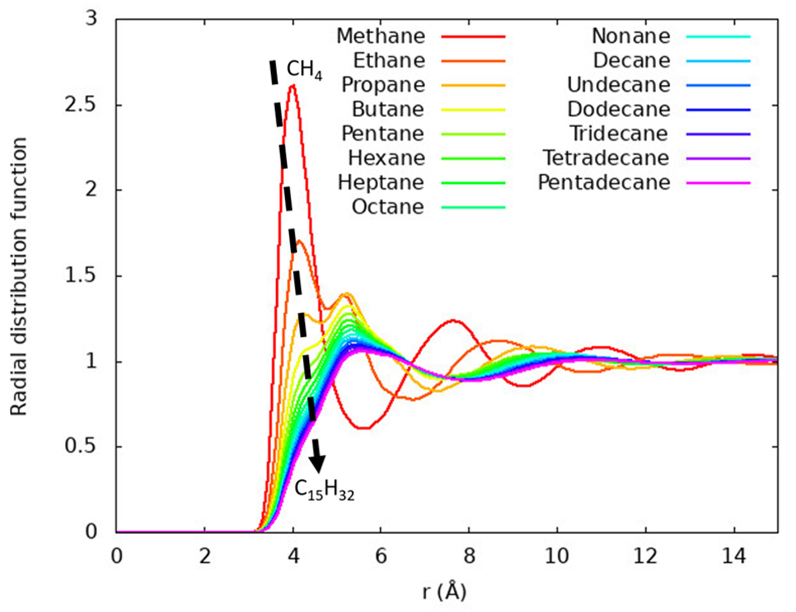
Figure 3 shows the carbon-carbon radial distribution function of each n-alkane liquid at its respective normal boiling point. In these, the radial distribution function is calculated between all carbons. Methane has a prominent maximum at about 4 Å that corresponds to the most likely separation between nearest neighbor pairs of methane molecules. This is like other studies of liquid methane and other molecules well described as a spherical Lennard-Jones particle [15,37,38,39]. The longer alkanes have peaks at about 4 and 5 Å. For ethane, the ~4 Å peak is larger in magnitude than the ~5 Å peak, but from propane to larger alkanes the ~5 Å peak is found to be larger in magnitude. For the longest alkanes considered, the ~4 Å peak becomes difficult to distinguish from the ~5 Å feature. It is common for short entries in a homologous molecular series to have distinct fluid behavior [40].
4.3. Local Structure in N-Alkane Liquids
The process of averaging over all carbon atoms in a system can obscure features arising from molecular arrangements specific to certain regions of the molecule. In Figure 4, we show the radial distribution function of each carbon progressing from the terminal carbon (Figure 4a) to the interior carbons. The short alkanes are still seen to be distinct, but they become more similar as the alkane length increases. Interestingly, the terminal carbon atoms are seen to have a more distinct ~4 Å peak for all alkanes, though this feature is less pronounced for the longer alkanes. The interior, non-terminal carbon atoms are generally observed to have similar local environments. At lower temperatures, this may provide insight into the nucleation process for n-alkanes as they crystallize, since the nucleation process in n-alkanes is known to entail elongation of the chains and then alignment to form the crystal lattice [41]. The distinct structure observed near the chain ends would likely be a useful metric for understanding phase transitions in these systems.
4.4. Thermodynamics of Binding
The radial distribution function reveals information about the spherically averaged intermolecular structure of the system, with the RDF maximum corresponding to the most likely separation of the pair of particles analyzed. ‘Inversion’ of the radial distribution function according to Equation (3) yields the free energy surface governing the behavior of that pair of particles. Therefore, the maximum in the radial distribution function corresponds to a minimum in the free energy of binding. This quantity is related to the work required to bring two particles together from infinite separation. Figure 5a shows that ΔGbind between carbon atoms becomes more positive with the increasing length of the alkane. Similar to the distinct shape of the radial distribution functions, CH4 and C2H6, the short alkanes, are observed to have ΔGbind values distinct from the longer alkanes. After C3H8, ΔGbind is found to increase less steeply, following an apparently different trend. This change in slope corresponds to the shift in the most prominent peak from ~4 to ~5 Å in the radial distribution function seen in Figure 3, showing that not only does the local structure shift but also the strength with which neighbors bind each other.
In Figure 5b, we examine the entropy change associated with this process. Like the discussion of ΔGbind in the previous paragraph, ΔSbind is related to the change in entropy when a molecule is taken from infinite separation into the condensed phase. The ΔSbind is found to generally decrease with increasing molecule length. Interestingly, ΔSbind is positive for small alkanes, from methane to pentane, but then crosses over to become negative from hexane on. The trends in structure of n-alkanes are closely linked to their increasing flexibility with length [25,42,43]. Feng et al. showed that there is a smooth trend in structural properties that can be partially understood from the context of the flexibility of the n-alkane chain [25]. The shorter alkanes have minimal variation in their length, as measured for example by radius of gyration or end-to-end length [25], but this molecular flexibility plays an increasingly important role in the structural properties of longer n-alkanes. There is not a distinct transition point from inflexible to flexible, but rather increasing flexibility with chain length like the trend seen in Figure 5b.
4.5. Consideration of Longer N-Alkanes
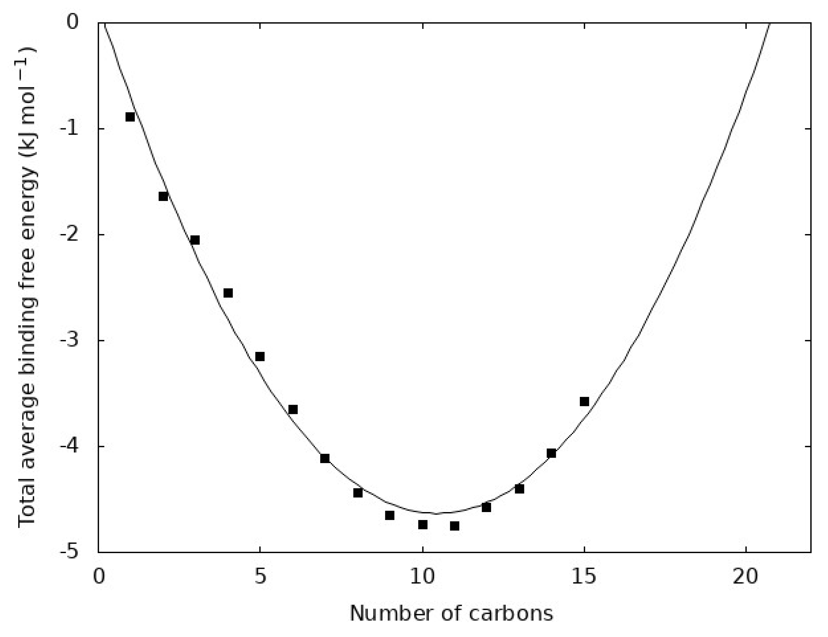
The quantity ΔGbind is related to the free energy holding one carbon atom from a given n-alkane in the liquid. Each molecule, however, contains n carbon atoms, so it is natural to assume that n ΔGbind can be a measure of the average total free energy holding a molecule within the liquid. This quantity is shown in Figure 6 for each n-alkane. We observe that it is well fit by a quadratic function. The line in Figure 6 extrapolates the total average binding free energy to determine the chain length where the free energy is zero. This yields roots of 0 and 21, which are the closest integer values. The value 21 corresponds to C21H44 and it is interesting to note that other studies have found dramatic changes in the dynamics and kinetics near this chain length. This is further evidenced by the fact that paraffin waxes are primarily composed of alkanes ranging from 20 to 40 carbon atoms [1,44,45] and this extrapolated point in our data near C20H42 may be unique evidence of a transition in the n-alkane series from small molecule to polymer-like behavior.
It is tempting to assume that n-alkanes beyond pentadecane could be estimated by simply extrapolating from the trends outlined here to longer n-alkanes. This is expected to be true to some extent, but at some point, there is a crossover from small molecule-like behavior to polymer-like behavior. Such a transition is often characterized by slowed molecular transport (often quantified by viscosity or molecular diffusion constant) induced by entanglement of the polymer chains. This transition has been observed to occur in n-alkanes slightly longer than the ones examined here [41], which also fits with broader polymer theory [46]. However, since this study focuses on behavior at the boiling point, polymer-like behavior would be unlikely to manifest even if modestly longer n-alkanes are considered.
5. Conclusions
We have found that GAFF2 with charges parameterized with RESP reproduces liquid densities at the normal boiling point of n-alkanes from methane to pentadecane within an average deviation of 2%. All deviations in density are positive but deviations in are more complex. is overestimated for short alkanes but the increase with chain length is too small so it is underestimated for long alkanes. This suggests that revisiting the parameterization of aliphatic molecules could be a way to improve this force field for these types of molecules. We examine the local structure and resulting thermodynamics and show that the shortest n-alkanes have a distinct liquid structure, but based on radial distribution functions, the series is found to converge to similar distribution functions for longer alkane chains. Further, we found that the molecular structure around terminal carbon atoms depends sensitively on the chain length, but interior carbon atoms have a more uniform local solvation structure. Finally, we found that the binding free energy between carbon atoms becomes less favorable with increasing chain length. The longer alkanes have more carbon atoms “holding” onto each other, so the net free energy holding molecules in the condensed phase does not necessarily become less favorable.
This study supports using GAFF2 to model these systems, despite the disparity in some cases between the environments and physical conditions envisioned when the force field was developed. There are undeniably specialized force fields [22,47,48] or even less empirical methods like ab initio molecular dynamics that can be used for these systems, but there are advantages to GAFF2. The diverse range of molecules that can be described by GAFF2, or conversely the difficulty of parameterizing new molecules or functional groups within the framework of more sophisticated force fields, makes GAFF2 a useful tool for atypical molecules. Additionally, since GAFF2 employs relatively simple functional forms, it can feasibly consider larger systems, which are often beyond practical limits for more computationally intensive methods. Therefore, approaches like those that we have presented here are an important tool for studying complex, heterogeneous systems like those where alkanes often occur.
Author Contributions
Conceptualization, G.E.L., J.L.B., J.H. and W.M.G.; methodology, G.E.L. and J.L.B.; validation, G.E.L. and C.K.; formal analysis, G.E.L.; investigation, G.E.L. and C.K.; resources, G.E.L. and J.LB.; data curation, G.E.L. and J.L.B.; writing—original draft preparation, G.E.L.; writing—review and editing, G.E.L., J.LB., J.H., W.M.G. and C.K.; visualization, G.E.L.; supervision, G.E.L.; project administration, G.E.L., J.H. and W.M.G.; funding acquisition, G.E.L., J.H. and W.M.G. All authors have read and agreed to the published version of the manuscript.
Funding
This research was partially funded by NASA, under grant numbers SSW-80NSSC18K0203 and SSW-80NSSC19K0556. The simulation setup and analysis were mostly performed on the Northern Arizona University supercomputer, Monsoon. The quantum chemistry calculations were performed on The College of New Jersey’s ELSA high performance computing cluster. This cluster is funded by the National Science Foundation under grant numbers OAC-1828163 and OAC-1826915.
Data Availability Statement
The information required to reproduce the simulations and all thermodynamic properties are provided within the article.
Conflicts of Interest
The authors declare no conflict of interest. The funders had no role in the design of the study; in the collection, analyses, or interpretation of data; in the writing of the manuscript, or in the decision to publish the results.
References
- Freund, M.; Csikos, R.; Keszthelyi, S.; Mozes, G. Paraffin Products; Properties, Technologies, Applications; Elsevier Scientific Publishing Company: Amsterdam, The Netherlands, 1982. [Google Scholar]
- Mango, F.D. The Light Hydrocarbons in Petroleum: A Critical Review. Org. Geochem. 1997, 26, 417–440. [Google Scholar] [CrossRef]
- Saunois, M.; Stavert, A.R.; Poulter, B.; Bousquet, P.; Canadell, J.G.; Jackson, R.B.; Raymond, P.A.; Dlugokencky, E.J.; Houweling, S.; Patra, P.K.; et al. The Global Methane Budget 2000–2017. Earth Syst. Sci. Data 2020, 12, 1561–1623. [Google Scholar] [CrossRef]
- Jackson, R.B.; Saunois, M.; Bousquet, P.; Canadell, J.G.; Poulter, B.; Stavert, A.R.; Bergamaschi, P.; Niwa, Y.; Segers, A.; Tsuruta, A. Increasing Anthropogenic Methane Emissions Arise Equally from Agricultural and Fossil Fuel Sources. Environ. Res. Lett. 2020, 15, 071002. [Google Scholar] [CrossRef]
- Cruikshank, D.P.; Pendleton, Y.J.; Grundy, W.M. Organic Components of Small Bodies in the Outer Solar System: Some Results of the New Horizons Mission. Life 2020, 10, 126. [Google Scholar] [CrossRef] [PubMed]
- MacKenzie, S.M.; Birch, S.P.D.; Horst, S.; Sotin, C.; Barth, E.; Lora, J.M.; Trainer, M.G.; Corlies, P.; Malaska, M.J.; Sciamma-O’Brien, E.; et al. Titan: Earth-like on the Outside, Ocean World on the Inside. Planet. Sci. J. 2021, 2, 112. [Google Scholar] [CrossRef]
- Engle, A.E.; Hanley, J.; Dustrud, S.; Thompson, G.; Lindberg, G.E.; Grundy, W.M.; Tegler, S.C. Phase Diagram for the Methane-Ethane System and Its Implications for Titan’s Lakes. Planet. Sci. J. 2021, 2, 118. [Google Scholar] [CrossRef]
- Hillyer, M.B.; Gibb, B.C. Molecular Shape and the Hydrophobic Effect. Annu. Rev. Phys. Chem. 2016, 67, 307–329. [Google Scholar] [CrossRef] [Green Version]
- Papavasileiou, K.D.; Peristeras, L.D.; Bick, A.; Economou, I.G. Molecular Dynamics Simulation of Pure N-Alkanes and Their Mixtures at Elevated Temperatures Using Atomistic and Coarse-Grained Force Fields. J. Phys. Chem. B 2019, 123, 6229–6243. [Google Scholar] [CrossRef] [PubMed]
- Nicholls, A.; Sharp, K.A.; Honig, B. Protein Folding and Association: Insights from the Interfacial and Thermodynamic Properties of Hydrocarbons. Proteins 1991, 11, 281–296. [Google Scholar] [CrossRef]
- Goodsaid-Zalduondo, F.; Engelman, D.M. Conformation of Liquid N-Alkanes. Biophys. J. 1981, 35, 587–594. [Google Scholar] [CrossRef] [Green Version]
- Izvekov, S.; Voth, G.A. A Multiscale Coarse-Graining Method for Biomolecular Systems. J. Phys. Chem. B 2005, 109, 2469–2473. [Google Scholar] [CrossRef]
- Klauda, J.B.; Brooks, B.R.; MacKerell, A.D., Jr.; Venable, R.M.; Pastor, R.W. An Ab Initio Study on the Torsional Surface of Alkanes and Its Effect on Molecular Simulations of Alkanes and a DPPC Bilayer. J. Phys. Chem. B 2005, 109, 5300–5311. [Google Scholar] [CrossRef] [PubMed]
- Bochyński, Z.; Drozdowsκi, H. Structure and Molecular Correlation of Liquid Alkanes. Acta Phys. Pol. A 1995, 88, 1089–1096. [Google Scholar] [CrossRef]
- Habenschuss, A.; Johnson, E.; Narten, A.H. X-ray Diffraction Study and Models of Liquid Methane at 92 K. J. Chem. Phys. 1981, 74, 5234–5241. [Google Scholar] [CrossRef]
- Sandler, S.I.; Lombardo, M.G.; Wong, D.S.-H.; Habenschuss, A.; Narten, A.H. X-ray Diffraction Study and Models of Liquid Ethane at 105 and 181 K. J. Chem. Phys. 1982, 77, 2144–2152. [Google Scholar] [CrossRef]
- Habenschuss, A.; Narten, A.H. X-ray Diffraction Study of Liquid Propane at 92 and 228 K. J. Chem. Phys. 1986, 85, 6022–6026. [Google Scholar] [CrossRef]
- Habenschuss, A.; Narten, A.H. X-ray Diffraction Study of Liquid N-butane at 140 and 267 K. J. Chem. Phys. 1989, 91, 4299–4306. [Google Scholar] [CrossRef]
- Bochyński, Z.; Drozdowski, H. X-Ray Scattering in Liquid Pentane. Phys. Chem. Liq. 2001, 39, 189–199. [Google Scholar] [CrossRef]
- Jorgensen, W.L.; Maxwell, D.S.; Tirado-Rives, J. Development and Testing of the OPLS All-Atom Force Field on Conformational Energetics and Properties of Organic Liquids. J. Am. Chem. Soc. 1996, 118, 11225–11236. [Google Scholar] [CrossRef]
- Luettmer-Strathmann, J.; Schoenhard, J.A.; Lipson, J.E.G. Thermodynamics of N-Alkane Mixtures and Polyethylene−n-Alkane Solutions: Comparison of Theory and Experiment. Macromolecules 1998, 31, 9231–9237. [Google Scholar] [CrossRef]
- Sun, H. COMPASS: An Ab Initio Force-Field Optimized for Condensed-Phase ApplicationsOverview with Details on Alkane and Benzene Compounds. J. Phys. Chem. B 1998, 102, 7338–7364. [Google Scholar] [CrossRef]
- Schuler, L.D.; Daura, X.; van Gunsteren, W.F. An Improved GROMOS96 Force Field for Aliphatic Hydrocarbons in the Condensed Phase. J. Comput. Chem. 2001, 22, 1205–1218. [Google Scholar] [CrossRef]
- Wang, J.; Hou, T. Application of Molecular Dynamics Simulations in Molecular Property Prediction I: Density and Heat of Vaporization. J. Chem. Theory Comput. 2011, 7, 2151–2165. [Google Scholar] [CrossRef] [PubMed] [Green Version]
- Feng, H.; Gao, W.; Su, L.; Sun, Z.; Chen, L. MD Simulation Study of the Diffusion and Local Structure of N-Alkanes in Liquid and Supercritical Methanol at Infinite Dilution. J. Mol. Model. 2017, 23, 195. [Google Scholar] [CrossRef] [PubMed]
- Gyawali, G.; Sternfield, S.; Kumar, R.; Rick, S.W. Coarse-Grained Models of Aqueous and Pure Liquid Alkanes. J. Chem. Theory Comput. 2017, 13, 3846–3853. [Google Scholar] [CrossRef] [PubMed]
- Schmidt, J.R.; Polik, W.F. WebMO Enterprise; WebMO LLC: Holland, MI, USA, 2020. [Google Scholar]
- Frisch, M.J.; Trucks, G.W.; Schlegel, H.B.; Scuseria, G.E.; Robb, M.A.; Cheeseman, J.R.; Scalmani, G.; Barone, V.; Petersson, G.A.; Nakatsuji, H.; et al. Gaussian16; Gaussian Inc.: Wallingford, CT, USA, 2016. [Google Scholar]
- Bayly, C.I.; Cieplak, P.; Cornell, W.; Kollman, P.A. A Well-Behaved Electrostatic Potential Based Method Using Charge Restraints for Deriving Atomic Charges: The RESP Model. J. Phys. Chem. 1993, 97, 10269–10280. [Google Scholar] [CrossRef]
- Case, D.A.; Belfon, K.; Ben-Shalom, I.; Brozell, S.R.; Cerutti, D.; Cheatham, T.; Cruzeiro, V.W.; Darden, T.; Duke, R.E.; Giambasu, G.; et al. Amber 2020; University of California: San Francisco, CA, USA, 2020. [Google Scholar]
- Wang, J.; Wolf, R.M.; Caldwell, J.W.; Kollman, P.A.; Case, D.A. Development and Testing of a General Amber Force Field. J. Comput. Chem. 2004, 25, 1157–1174. [Google Scholar] [CrossRef] [PubMed]
- Martínez, L.; Andrade, R.; Birgin, E.G.; Martínez, J.M. PACKMOL: A Package for Building Initial Configurations for Molecular Dynamics Simulations. J. Comput. Chem. 2009, 30, 2157–2164. [Google Scholar] [CrossRef] [PubMed]
- Burgess, D.R., Jr. Thermochemical Data. In NIST Chemistry WebBook; Linstrom, P.J., Mallard, W.G., Eds.; National Institute of Standards and Technology: Gaithersburg, MD, USA, 2021. [Google Scholar]
- Roe, D.R.; Cheatham, T.E. PTRAJ and CPPTRAJ: Software for Processing and Analysis of Molecular Dynamics Trajectory Data. J. Chem. Theory Comput. 2013, 9, 3084–3095. [Google Scholar] [CrossRef] [PubMed]
- Tobler, F.C. Correlation of the Density of the Liquid Phase of Pure N-Alkanes with Temperature and Vapor Pressure. Ind. Eng. Chem. Res. 1998, 37, 2565–2570. [Google Scholar] [CrossRef]
- Caleman, C.; van Maaren, P.J.; Hong, M.; Hub, J.S.; Costa, L.T.; van der Spoel, D. Force Field Benchmark of Organic Liquids: Density, Enthalpy of Vaporization, Heat Capacities, Surface Tension, Isothermal Compressibility, Volumetric Expansion Coefficient, and Dielectric Constant. J. Chem. Theory Comput. 2012, 8, 61–74. [Google Scholar] [CrossRef]
- Tchouar, N.; Benyettou, M.; Kadour, F.O. Thermodynamic, Structural and Transport Properties of Lennard-Jones Liquid Systems. A Molecular Dynamics Simulations of Liquid Helium, Neon, Methane and Nitrogen. Int. J. Mol. Sci. 2003, 4, 595–606. [Google Scholar] [CrossRef] [Green Version]
- Tchouar, N.; Benyettou, M.; Baghli, H. A Reversible Algorithm for Nosé Molecular Dynamics Simulations. Equilibrium Properties of Liquid Methane. J. Mol. Liq. 2007, 136, 5–10. [Google Scholar] [CrossRef]
- Petz, J.I. X-Ray Determination of the Structure of Liquid Methane. J. Chem. Phys. 1965, 43, 2238–2243. [Google Scholar] [CrossRef]
- Assael, M.J.; Dymond, J.H.; Exadaktilou, D. An Improved Representation Forn-Alkane Liquid Densities. Int. J. Thermophys. 1994, 15, 155–164. [Google Scholar] [CrossRef]
- Kraack, H.; Deutsch, M.; Sirota, E.B. N-Alkane Homogeneous Nucleation: Crossover to Polymer Behavior. Macromolecules 2000, 33, 6174–6184. [Google Scholar] [CrossRef]
- Lal, M.; Spencer, D. “Monte Carlo” Computer Simulation of Chain Molecules. Mol. Phys. 1973, 26, 1–6. [Google Scholar] [CrossRef]
- Romain, P.D.; Van, H.T.; Patterson, D. Effects of Molecular Flexibility and Shape on the Excess Enthalpies and Heat Capacities of Alkane Systems. J. Chem. Soc. Lond. Faraday Trans. 1 1979, 75, 1700–1707. [Google Scholar] [CrossRef]
- Sanjay, M.; Simanta, B.; Kulwant, S. Paraffin Problems in Crude Oil Production and Transportation: A Review. SPE Prod. Facil. 1995, 10, 50–54. [Google Scholar] [CrossRef]
- Anufriev, R.V.; Volkova, G.I.; Vasilyeva, A.A.; Petukhova, A.V.; Usheva, N.V. The Integrated Effect on Properties and Composition of High-Paraffin Oil Sludge. Procedia Chem. 2015, 15, 2–7. [Google Scholar] [CrossRef] [Green Version]
- Ding, Y.; Kisliuk, A.; Sokolov, A.P. When Does a Molecule Become a Polymer? Macromolecules 2004, 37, 161–166. [Google Scholar] [CrossRef]
- Martin, M.G.; Siepmann, J.I. Transferable Potentials for Phase Equilibria. 1. United-Atom Description of N-Alkanes. J. Phys. Chem. B 1998, 102, 2569–2577. [Google Scholar] [CrossRef]
- Martin, M.G. Comparison of the AMBER, CHARMM, COMPASS, GROMOS, OPLS, TraPPE and UFF Force Fields for Prediction of Vapor–liquid Coexistence Curves and Liquid Densities. Fluid Phase Equilib. 2006, 248, 50–55. [Google Scholar] [CrossRef]
Figure 1.
Density of each n-alkane liquid at the respective experimental normal boiling point of each molecule.
Figure 1.
Density of each n-alkane liquid at the respective experimental normal boiling point of each molecule.
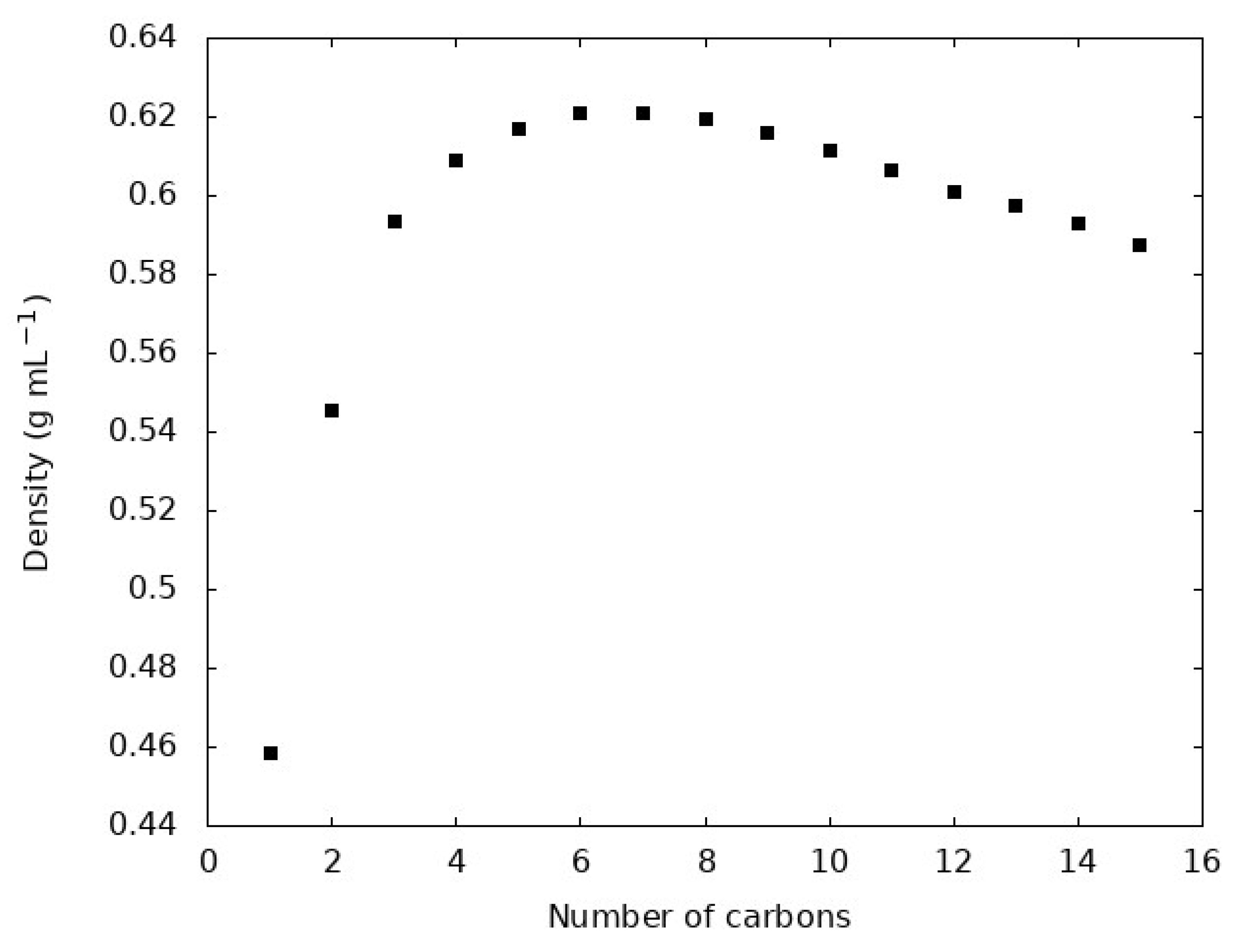
Figure 2.
Comparison of experimental and simulated densities. The line along the diagonal is indicative of perfect agreement between experimental and simulated values, so points above the line represent the simulations overestimating the density of a liquid. The experimental n-alkane densities are obtained from Tobler [35]. The colors indicate the molecule and are the same as Figure 3. The largest deviation is observed for CH4 with the simulations overestimating the density by 8%. All simulations result in higher densities than the experimental results, with an average deviation of 1.9% across all liquids.

Figure 3.
Radial distribution functions between all carbon atoms for each n-alkane excluding intramolecular pairs. The radial distribution functions have prominent peaks near 4 and 5 Å, with longer alkane chain lengths corresponding to increased prominence of the ~5 Å peak. Longer alkanes are seen to converge to generally similar distribution functions. The dashed arrow indicates the convergence from sharply peaked methane to the less structured distribution of pentadecane.

Figure 4.
Radial distribution functions between specific carbons and all other carbons. Intramolecular pairs are excluded. The first panel (a) is the radial distribution function from the terminal carbon(s) to all other carbons, the second panel (b) is the carbon(s) next to the terminal carbon to all other carbons, the third panel (c) is the second carbon(s) from the terminal carbon to all other carbons, the fourth panel (d) is the third carbon(s) from the terminal carbon to all other carbons, the fifth panel (e) is the fourth carbon(s) from the terminal carbon to all other carbons, the sixth panel (f) is the fifth carbon(s) from the terminal carbon to all other carbons, the seventh panel (g) is the sixth carbon(s) from the terminal carbon to all other carbons, and the eighth panel (h) is the seventh carbon from the terminal carbon to all other carbons. The colors indicate the molecule and are the same as Figure 3. Only distinct radial distribution functions are shown, so only one ethane radial distribution function is included because the two carbon atoms are symmetrically equivalent. The radial distribution functions are observed to be more structured near the terminal carbons and become progressively smoother for interior carbon atoms.
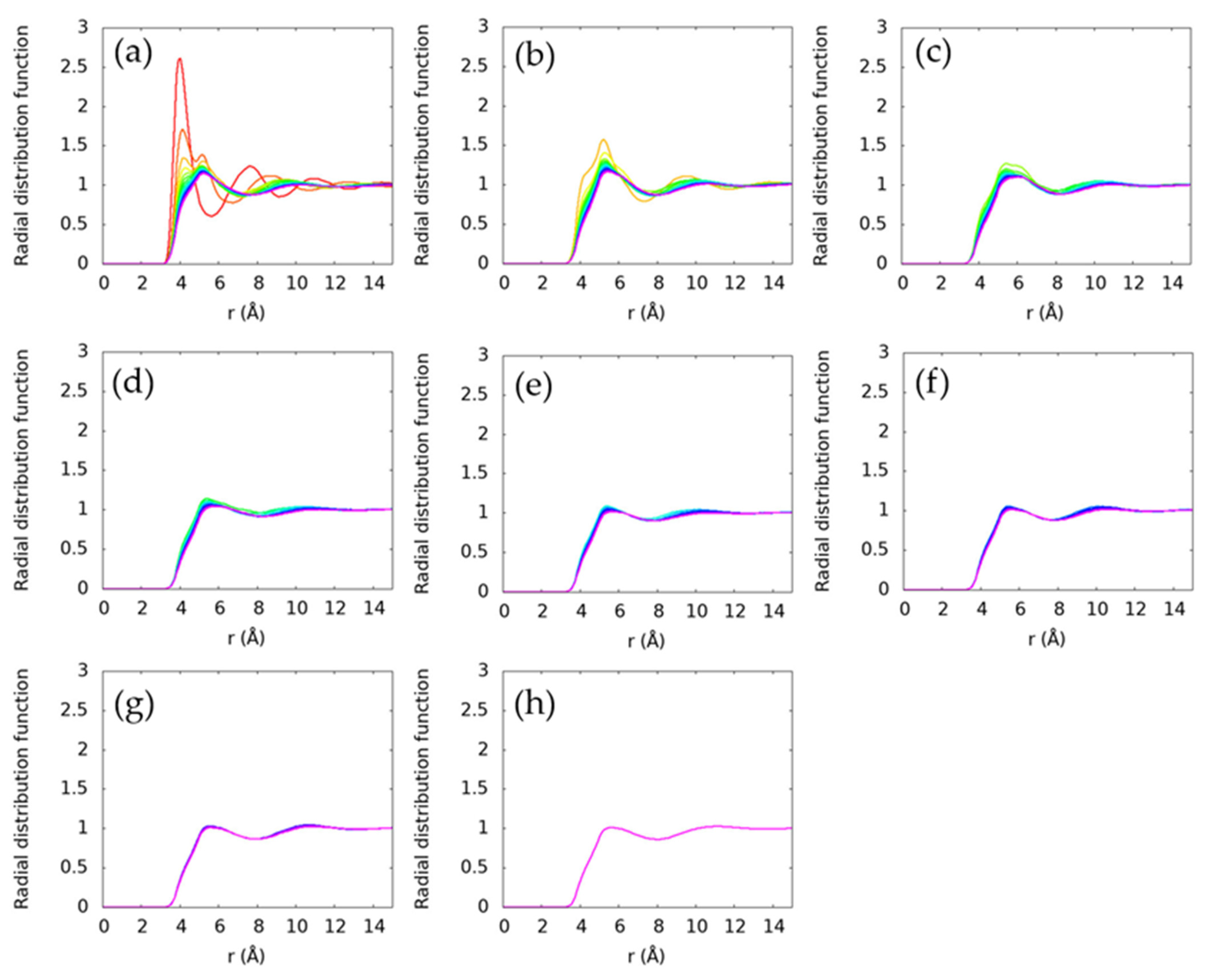
Figure 5.
Free energy (a) and entropy (b) of binding for each n-alkane at the boiling point of each molecule. The free energy of binding, ΔGbind, is determined from the maximum in the carbon radial distribution functions shown in Figure 3. The entropy of binding, ΔSbind, is numerically estimated using the binding free energy in panel (a) and similar analysis of another simulation 10 K below the boiling point.

Figure 6.
Total average binding free energy for each n-alkane. The total average binding free energy is n ΔGbind where n is the number of carbon atoms in the molecule and ΔGbind is from Figure 5a. The points show the value for each n-alkane and the line is a best fit quadratic function.
Figure 6.
Total average binding free energy for each n-alkane. The total average binding free energy is n ΔGbind where n is the number of carbon atoms in the molecule and ΔGbind is from Figure 5a. The points show the value for each n-alkane and the line is a best fit quadratic function.


Table 1.
Experimental boiling points of each species at 1 bar.
| Molecule | Boiling Point (K) a |
|---|---|
| Methane | 111. ± 2 |
| Ethane | 184.6 ± 0.6 |
| Propane | 231.1 ± 0.2 |
| Butane | 273. ± 1 |
| Pentane | 309.2 ± 0.2 |
| Hexane | 341.9 ± 0.3 |
| Heptane | 371.5 ± 0.3 |
| Octane | 398.7 ± 0.5 |
| Nonane | 423.8 ± 0.3 |
| Decane | 447.2 ± 0.3 |
| Undecane | 468. ± 2 |
| Dodecane | 489. ± 2 |
| Tridecane | 507. ± 2 |
| Tetradecane | 523. ± 10 |
| Pentadecane | 540. ± 20 |
a Boiling points are obtained from the NIST Thermochemical database [33].
Table 2.
Simulated and experimental enthalpy of vaporization, , for each n-alkane at the respective boiling point.
Table 2.
Simulated and experimental enthalpy of vaporization, , for each n-alkane at the respective boiling point.
| Molecule | Simulated | Experiment a | Percent Difference |
|---|---|---|---|
| Methane | 2.33 ± 0.02 | 2.06 | 13% |
| Ethane | 3.88 ± 0.05 | 3.75 | 3% |
| Propane | 5.25 ± 0.08 | 4.55 | 15% |
| Butane | 6.5 ± 0.1 | 5.47 | 20% |
| Pentane | 7.3 ± 0.1 | 6.33 | 16% |
| Hexane | 8.3 ± 0.2 | 7.41 | 13% |
| Heptane | 9.4 ± 0.2 | 8.60 | 10% |
| Octane | 10.2 ± 0.2 | 9.80 | 4% |
| Nonane | 11.1 ± 0.2 | 11.11 | 0.3% |
| Decane | 12.2 ± 0.3 | 12.26 | −0.4% |
| Undecane | 12.1 ± 0.3 | 13.48 | −10% |
| Dodecane | 13.1 ± 0.3 | 14.58 | −10% |
| Tridecane | 13.9 ± 0.3 | 15.94 | −13% |
| Tetradecane | 14.9 ± 0.4 | 17.11 | −13% |
| Pentadecane | 15.6 ± 0.4 | 18.19 | −14% |
a Experimental values are obtained from the NIST Thermochemical database [33].
Publisher’s Note: MDPI stays neutral with regard to jurisdictional claims in published maps and institutional affiliations. |
© 2021 by the authors. Licensee MDPI, Basel, Switzerland. This article is an open access article distributed under the terms and conditions of the Creative Commons Attribution (CC BY) license (https://creativecommons.org/licenses/by/4.0/).
Share and Cite
MDPI and ACS Style
Lindberg, G.E.; Baker, J.L.; Hanley, J.; Grundy, W.M.; King, C. Density, Enthalpy of Vaporization and Local Structure of Neat N-Alkane Liquids. Liquids 2021, 1, 47-59. https://0-doi-org.brum.beds.ac.uk/10.3390/liquids1010004
AMA Style
Lindberg GE, Baker JL, Hanley J, Grundy WM, King C. Density, Enthalpy of Vaporization and Local Structure of Neat N-Alkane Liquids. Liquids. 2021; 1(1):47-59. https://0-doi-org.brum.beds.ac.uk/10.3390/liquids1010004
Chicago/Turabian StyleLindberg, Gerrick E., Joseph L. Baker, Jennifer Hanley, William M. Grundy, and Caitlin King. 2021. "Density, Enthalpy of Vaporization and Local Structure of Neat N-Alkane Liquids" Liquids 1, no. 1: 47-59. https://0-doi-org.brum.beds.ac.uk/10.3390/liquids1010004