Article

A Co-Infection Model for Onchocerciasis and Lassa Fever with Optimal Control Analysis

by
Kabiru Michael Adeyemo
1,
Kayode Oshinubi
2,
Umar Muhammad Adam
3 and
Adejimi Adeniji
4,*
1
Department of Mathematics, Hallmark University, Ijebu-Itele 122101, Nigeria
2
School of Informatics, Computing, and Cyber Systems, Northern Arizona University, Flagstaff, AZ 86011, USA
3
Department of Mathematics, Federal University, Dutse 720222, Nigeria
4
Department of Mathematics and Statistics, Tshwane University of Technology, Pretoria 0083, South Africa
*
Author to whom correspondence should be addressed.
Submission received: 24 October 2023 / Revised: 16 December 2023 / Accepted: 5 January 2024 / Published: 10 January 2024

Abstract

:
A co-infection model for onchocerciasis and Lassa fever (OLF) with periodic variational vectors and optimal control is studied and analyzed to assess the impact of controls against incidence infections. The model is qualitatively examined in order to evaluate its asymptotic behavior in relation to the equilibria. Employing a Lyapunov function, we demonstrated that the disease-free equilibrium (DFE) is globally asymptotically stable; that is, the related basic reproduction number is less than unity. When it is bigger than one, we use a suitable nonlinear Lyapunov function to demonstrate the existence of a globally asymptotically stable endemic equilibrium (EE). Furthermore, the necessary conditions for the presence of optimum control and the optimality system for the co-infection model are established using Pontryagin’s maximum principle. The model is quantitatively analyzed by studying how sensitive the basic reproduction number is to the model parameters and the model simulation using Runge–Kutta technique of order 4 is also presented to study the effects of the treatments. We deduced from the quantitative analysis that, if there is an effective treatment and diagnosis of those exposed to and infected with the disease, the spread of the viral disease can be effectively managed. The results presented in this work will be useful for the proper mitigation of the disease.

1. Introduction

Onchocerciasis is a neglected tropical illness caused by the filarial worm parasite Onchocerca Volvulus [1,2,3,4]. The disease is spread from person to person through frequent bites from black flies, and is particularly prevalent in sub-Saharan Africa. However, another word for it is riverine blindness, which infers that the disease burden is higher in regions near rivers, as the presence of riverine hatching sites for black flies has a substantial impact on the incidence of onchocerciasis infection in a community. The disease is more common in adults under the age of 30. Many researchers have worked on numerous ways of reducing the spread of the disease using different modeling approaches, both mathematically and statistically, suggesting ways of mitigating the disease. The modeling of different kinds of viral diseases extended to optimal control and the study of the co-infection of infectious disease dynamics have been the subjects of several studies (see [5,6,7,8,9,10,11,12]). In [2], the authors used a computer algebra system (CAS) simulation procedure to study the model to prevent onchocerciasis using macrofilaricide, which kills the adult worms. The study provided in [3] looked at the effects of four distinct methods of control on disease spread. Ref. [13] used a microsimulation model to assess the time required to combine annual ivermectin therapy and vector control in the West African onchocerciasis Control Programme. For example, in [14], scientists performed a skin snip survey in west Africa to assess the impact of larviciding on the suppression of black flies. The Arena virus (Lassa virus) causes Lassa fever, a viral disease. It is zoonotic and acute, causing severe hemorrhagic fever with symptoms like nausea, sore throat, vomiting, chest and stomach discomfort, muscle cramps, fever, and ocular discharges. When humans come into contact with the virus on these contaminated surfaces, they can become infected indirectly. Rodents can also become infected because they share rubbish, eat on surfaces polluted with infectious rodent excretions, and do not die from disease but carry the infection and continue to spread it throughout their lives. Infections can be regularly diagnosed throughout the year; however, peak times in tropical regions have been seen between January and May throughout the period of drought [15,16,17]. Ref. [15] created a mathematical representation of Lassa fever transmission and dynamics in two interacting populations. In another breakthrough, [18] created a mathematical model for Lassa fever transmission dynamics, examined endemic stability, determined the stability of the disease-free equilibrium, and estimated the threshold value. Our work is motivated based on the research in [19], wherein the authors consider the co-infection model of malaria–Lassa using optimal control. The developed model reflected seasonal fluctuation in vectors and showed that co-infection with malaria and Lassa fever increased mortality in infected patients. Research on the optimal control of the co-infection of diseases has been highly explored; however, to the best of the authors’ understanding, optimal control analysis is not currently used in the literature to study the co-infection of onchocerciasis and Lassa fever. This study investigates the global stability properties and optimal control analysis of onchocerciasis–Lassa fever co-infection in three interacting populations of humans (the host), black-flies (the vector), and rodents, which incorporate periodic variational vectors and diagnostic factors for the treatment of onchocerciasis–Lassa fever co-infection. To show the novelty of our work in this paper, and to the best of our knowledge, this is the first time that research has sought to understand the co-infection model for onchocerciasis and Lassa fever dynamics and its optimal control. We use a search engine procedure, such as Google scholar, Web of Science, and Scopus search, to validate the novelty of this research. The key findings of this research help us understand that, in the process of disease mitigation, treatment is more likely to reduce the infection. With the treatment procedure comes the tool of insecticides that also enhance the process of mitigation, i.e., this process has a positive implication in ensuring that the community is onchocerciasis–Lassa-free. Another mitigation method from this research is the optimal control investigation and sensitivity analysis. The optimal control and sensitivity analysis shows the effect of the control parameters on the basic reproduction number, which efficiently inform the public and health officials of the possibility of reducing the infection and transmission rates where the disease is predominant.
The remainder of the paper is structured as follows: Section 2 contains the model’s formulation as well as its basic features. Section 3 qualitatively analyzes the co-infection scenario without controls. Section 4 considers the optimal control model, whereas the numerical simulation of the model and the discussion of the results are presented in Section 5. The concluding remarks, limitations, future work, and key results are discussed in Section 6.

2. OLF Co-Infection Model

This work sought to study the transmission dynamics of OLF co-infection in three interacting populations of humans (the host), black flies (the vector), and rodents, which incorporate periodic variational vectors [19,20,21], because we know that zoonotic and vector-borne diseases have some environmental drivers and diagnostic factors for the treatment of onchocerciasis–Lassa fever co-infection, and we formulate a model which subdivides the total human and rodent population sizes at time t and discrete age c i and d j denoted by N h ( t , c i ) = N s s ( t , c i ) + N s e ( t , c i ) + N s i ( t , c i ) + N s r ( t , c i ) + N e s ( t , c i ) + N i s ( t , c i ) + N r s ( t , c i ) + N r r ( t , c i ) , N r ( t , d j ) = S r ( t , d j ) + E r ( t , d j ) + I r ( t , d j ) with i = 0 , 1 , 2 , . . . , L , j = 0 , 1 , 2 , . . . , T and c L and d T are the maximum age of humans and rodents in the population. Similarly, the total black fly population size at time t is denoted by N b ( t ) = S b ( t ) + E b ( t ) + I b ( t ) .
The state variables N s e ,   N s i and N s r denote the number of people in the human population that were exposed to Lassa fever, infected by Lassa fever, and recovered from Lassa fever, respectively, but susceptible to onchocerciasis. Moreover, N e s ,   N i s and N r s represents those exposed, infected and recovered from onchocerciasis, respectively, but susceptible to Lassa fever. It is imperative to note that N r r denotes the number of those that recovered from both diseases. However, N s s represents the number of those susceptible to both diseases. The rodent population was classified as S r ,   E r , and I r , representing those that were susceptible, exposed, and infected, respectively. Furthermore, the black fly population was classified as S b ,   E b , and I b , denoting those that were susceptible, exposed, and infected, respectively. Let λ B ( t ) = c 0 ( c i ) ( 1 + b cos ( 2 π t + T ) ) I b be the onchocerciasis infection rate, where c 0 ( c i ) = c b ( c i ) N h ( t , c i ) , b N h ( t , c i ) is the contact rate between humans and black flies, and b is the rate at which humans are being bitten by black flies. Similarly, λ a ( t ) = ρ 0 ( c i ) ( 1 + w 2 ( d j ) cos ( 2 π t + T ) ) I r ( t , d j ) and λ b ( t ) = σ 0 ( c i ) ( 1 + w 1 ( c i ) cos ( 2 π t + T ) ) N s i ( t , c i ) are the forces of infection for Lassa fever, where σ 0 = d 1 ( c i ) N h ( t , c i ) and ρ 0 = d 2 ( c i ) N h ( t , c i ) . In the black fly and rodent populations λ b ( t ) = ϕ 0 ( 1 + b cos ( 2 π t + T ) ) and λ r ( t ) = β 0 ( d j ) ( 1 + w 2 ( d j ) cos ( 2 π t + T ) ) , ϕ 0 = σ b N b and β 0 ( d j ) = β r ( d j ) N r ( t , d j ) . The subscripts r , b represent the Lassa fever (rodent) and onchocerciasis (black fly), respectively. Ribavirin (anti-viral drug) is effective when it is administered early. It is assumed that both exposed and infectious humans are treated at rates of γ 1 ( c i ) α ( c i ) N s e ( t , c i ) and η 1 ( c i ) σ ( c i ) N s i ( t , c i ) , respectively. N r r ( t , c i ) represents those who are infected with both diseases.
The formulation of the compartmental model is based on the following assumptions because of our knowledge of both diseases and the research performed in [19]:
  • Every person is born with the ability to catch Lassa fever and onchocerciasis, implying that humans are at risk of contracting the diseases.
  • Once susceptible people become sick, they transform into exposed people with immunity but are not yet contagious.
  • Only individuals who are exposed to the virus become contagious.
  • Infectious individuals can die naturally or as a consequence of the disease, and if they do otherwise, they can recover as a result of treatment.
  • That person could simultaneously contract both Lassa fever and onchocerciasis.
  • All rodents including black flies have vulnerability during birth.
  • Each type of rodent species may perish spontaneously or as a result of hunting and the application of pesticides.
  • Infected sensitive rodents are exposed but not contagious rodents.
  • Only exposed rodents and black flies become infected.
  • Infected rodents become infected when they consume or consume fluids from ill rodents.
  • Afflicted rodents and black flies are infectious for life, implying that there is no recovered class for rodent and black fly populations.
Following that, we obtain a 14-dimensional system of ODEs that explains disease spread as follows:
d N s s t , c i d t = ζ c i i = 0 L j = 0 T λ a + λ b N s s t , c i i = 0 L λ B N s s t , c i I b μ c i N s S t , c i + γ b c i N r S t , c i d N s e t , c i d t = i = 0 L j = 0 T λ a + λ b N S s t , c i i = 0 L ϑ b c i λ B N S e t , c i I b μ c i + γ v c i α c i + τ c i N S e t , c i d N s i t , c i d t = i = 0 L τ c i N s e t , c i i = 0 L ϑ b c i λ B N s i t , c i I b μ c i + η v c i σ c i N s i t , c i d N s r t , c i d t = i = 0 L γ v c i α c i N s e t , c i + η v c i σ c i N s i t , c i μ c i N s r t , c i d N e s t , c i d t = i = 0 L λ B N s s t , c i I b i = 0 L j = 0 T ϑ r c i λ a + λ b N e s t , c i μ c i + τ b c i N e S t , c i d N i s t , c i d t = i = 0 L τ b c i N e S t , c i i = 0 L j = 0 T ϑ r c i λ a + λ b N i S t , c i μ c i + ϵ b c i β b c i N i s t , c i d N r s t , c i d t = i = 0 L ϵ b c i β b c i N i s t , c i γ b c i + μ c i N r s t , c i d N r r t , c i d t = i = 0 L ϑ b c i λ B N s e t , c i + N s i t , c i I b μ c i N r r t , c i + i = 0 L j = 0 T ϑ r c i λ a + λ b N e s t , c i + N i s t , c i d S r t , d j d t = Λ r d j 1 + ξ r cos ( 2 π t + T ) j = 0 T λ r S r t , d j I r t , d j μ r d j + δ r d j S r t , d j d E r t , d j d t = j = 0 T λ r S r t , d j I r t , d j α r d j + μ r d j + δ r d j E r t , d j d I r t , d j d t = j = 0 T α r d j E r t , d j μ r d j + δ r d j I r t , d j d S b d t = ς b 1 + κ b cos ( 2 π t + T ) λ b S b N i s t , c i μ b S b d E b d t = λ b S b N i s t , c i μ b + α b E b d I b d t = α b E b μ b I b
and the ICs
N s s ( 0 , c i ) = N 0 s s ( c i ) , N s e ( 0 , c i ) = N 0 s e ( c i ) , N s i ( 0 , c i ) = N 0 s i ( c i ) , N s r ( 0 , c i ) = N 0 s r ( c i ) , N e s ( 0 , c i ) = N 0 e s ( c i ) , N i s ( 0 , c i ) = N 0 i s ( c i ) , N r s ( 0 , c i ) = N 0 r s ( c i ) , S r ( 0 , d j ) = S 0 r , E r ( 0 , d j ) = E 0 r , I r ( 0 , d j ) = I 0 r , S b ( 0 ) = S 0 b , E b ( 0 ) = E 0 b , I b ( 0 ) = I 0 b
In Table 1, we present the definition of the parameters of model (1), and in Table 2, we present the parameter values used for the quantitative aspect of the research.

Basic Model Features Model (1) without Controls

The respective results which guarantee the OLF-model co-infection model, governed by model (1), represent a mathematically well-posed and feasible region Ω defined by
Ω = Ω h × Ω r × Ω b R + 8 × R + 3 × R + 3
where Ω h = { N s s ( t , c i ) , N s e ( t , c i ) , N s i ( t , c i ) , N s r ( t , c i ) , N e s ( t , c i ) , N i s ( t , c i ) , N r s ( t , c i ) , N r r ( t , c i ) R 8 : N h ( t , c i ) i = 0 L ζ ( c i ) μ ( c i ) } ,
Ω r = { S r ( t , d j ) , E r ( t , d j ) , I r ( t , d j ) , R + 3 : N r ( t , d j ) j = 0 T Λ r ( d j ) ( 1 + ξ r cos ( 2 π t + T ) ) μ r ( d j ) + δ r ( d j ) }
and
Ω b = { S b ( t ) ,   E b ( t ) ,   I b ( t ) , R + 3 : N b ( t ) ς b ( 1 + κ b cos ( 2 π t + T ) ) μ b }
Theorem 1.
The feasible region Ω defined by Ω = { N s s ( t , c i ) , N s e ( t , c i ) , N s i ( t , c i ) , N s r ( t , c i ) , N e s ( t , c i ) , N i s ( t , c i ) , N r s ( t , c i ) , N r r ( t , c i ) , S r ( t , d j ) , E r ( t , d j ) , I r ( t , d j ) , S b ( t ) E b ( t ) , I b ( t ) R 14 : N h ( 0 , c i ) N h ( t , c i ) i = 0 L ζ ( c i ) μ ( c i ) , N r ( 0 , d j ) N r ( t , d j ) j = 0 T Λ r ( d j ) ( 1 + ξ r cos ( 2 π t + T ) ) μ r ( d j ) + δ r ( d j ) , N b ( 0 ) N b ( t ) ς b ( 1 + κ b cos ( 2 π t + T ) ) μ b } with IC’s N s s ( 0 , c i ) 0 , N s e ( 0 , c i ) 0 , N s i ( 0 , c i ) 0 , N s r ( 0 , c i ) 0 , N e s ( 0 , c i ) 0 , N i s ( 0 , c i ) 0 , N r s ( 0 , c i ) 0 , N r r ( 0 , c i ) 0 , S r ( 0 , d j ) 0 , E r ( 0 , d j ) 0 , I r ( 0 , d j ) 0 , S b ( 0 ) 0 , E b ( 0 ) 0 , I b ( 0 ) 0 is a non-negative variant for model (1).
Proof. 
If N h ( t , c i ) = N s s ( t , c i ) + N s e ( t , c i ) + N s i ( t , c i ) + N s r ( t , c i ) + N e s ( t , c i ) ,   N i s ( t , c i ) + N r s ( t , c i ) + N r r ( t , c i ) represent the sum of the population of human, the sum population of the rodent is N r ( t , d j ) = S r ( t , d j ) + E r ( t , d j ) + I r ( t , d j ) and the complete size of black fly community is N b ( t ) = S b ( t ) + E b + I b . Then, from model (1)
d N h ( t , c i ) d t ζ ( c i ) i = 0 L μ ( c i ) N h ( t , c i )
d N r d t Λ r ( d j ) ( 1 + ξ r cos ( 2 π t + T ) ) i = 0 L ( μ r ( d j ) + δ r ( d j ) ) N r ( t , d j )
d N b d t ς b ( 1 + κ b cos ( 2 π t + T ) ) μ b N b
Considering the inequalities of the ODE of (3), (4), and (5), respectively,
N h ( t , c i ) e μ h ( c i ) t N h ( 0 , c i ) + i = 0 L Λ ( c i ) μ h ( c i ) e μ h ( c i ) t i = 0 L Λ ( c i ) μ h ( c i )
so that
N h ( t , c i ) N h ( 0 , c i ) e μ h ( c i ) t + i = 0 L Λ ( c i ) μ h ( c i ) i = 0 L Λ ( c i ) μ h ( c i ) e μ h ( c i ) t
this implies
N h ( t , c i ) i = 0 L Λ ( c i ) μ h ( c i ) ( 1 e μ h ( c i ) t ) + N h ( 0 , c i ) e μ h ( c i ) t
similarly, for Equation (4), we have
N r ( t , d j ) e ( μ r ( d j ) + δ r ( d j ) ) t j = 0 T N r ( 0 , d j ) + Λ r ( d j ) ( 1 + ξ r cos ( 2 π t + T ) ) μ r ( d j ) + δ r ( d j ) e ( μ r ( d j ) + δ r ( d j ) ) t Λ r ( d j ) ( 1 + ξ r cos ( 2 π t + T ) ) μ r ( d j ) + δ r ( d j )
so that
N r ( t , d j ) j = 0 T N r ( 0 , d j ) e ( μ r ( d j ) + δ r ( d j ) ) t + Λ r ( d j ) ( 1 + ξ r cos ( 2 π t + T ) ) μ r ( d j ) + δ r ( d j ) Λ r ( d j ) ( 1 + ξ r cos ( 2 π t + T ) ) μ r ( d j ) + δ r ( d j ) e ( μ r ( d j ) + δ r ( d j ) ) t
this implies
N r ( t , d j ) j = 0 T Λ r ( d j ) ( 1 + ξ r cos ( 2 π t + T ) ) μ r ( d j ) + δ r ( d j ) ( 1 e ( μ r ( d j ) + δ r ( d j ) ) t ) + N r ( 0 , d j ) e ( μ r ( d j ) + δ r ( d j ) ) t
Also,
N b ( t ) e μ b t N b ( 0 ) + ς b ( 1 + κ b cos ( 2 π t + T ) ) μ b e μ b t ς b ( 1 + κ b cos ( 2 π t + T ) ) μ b
so that
N b ( t ) N b ( 0 ) e μ b t + Λ m μ b ς b ( 1 + κ b cos ( 2 π t + T ) ) μ b e μ b t
this implies
N b ( t ) ς b ( 1 + κ b cos ( 2 π t + T ) ) μ b ( 1 e μ b t ) + N b ( 0 ) e μ b t .
Taking the limits of Equations (6)–(8) as t gives N h ( t , c i ) i = 0 L ζ ( c i ) μ h ( c i ) , N r ( t , d j ) j = 0 T Λ r ( d j ) ( 1 + ξ r cos ( 2 π t + T ) ) μ r ( d j ) + δ r ( d j ) and N b ( t ) ς b ( 1 + κ b cos ( 2 π t + T ) ) μ b . Thus, the following feasible region Ω = { N s s ( t , c i ) ,   N s e ( t , c i ) ,   N s i ( t , c i ) ,   N s r ( t , c i ) ,   N e s ( t , c i ) , N i s ( t , c i ) ,   N r s ( t , c i ) ,   N r r ( t , c i ) ,   S r ( t , d j ) ,   E r ( t , d j ) ,   I r ( t , d j ) ,   S b ,   E b ,   I b R 14 : N h ( t , c i ) i = 0 L ζ ( c i ) μ ( c i ) , N r ( t , d j ) j = 0 T Λ r ( d j ) ( 1 + ξ r cos ( 2 π t + T ) ) μ r ( d j ) + δ r ( d j ) , N b ( t ) ς b ( 1 + κ b cos ( 2 π t + T ) ) μ b } . □

3. Analysis of Model (1) with Non-Controls

It is crucial to remember that, given the recruiting terms, there are no trivial equilibrium locations, ζ ( c i ) , Λ r ( d j ) ( 1 + ξ r cos ( 2 π t + T ) ) and Λ b ( 1 + ξ b cos ( 2 π t + T ) ) that are non-zero. This implies that the equilibrium points ( N s s ( t , c i ) ,   N s e ( t , c i ) ,   N s i ( t , c i ) ,   N s r ( t , c i ) ,   N e s ( t , c i ) , N i s ( t , c i ) ,   N r s ( t , c i ) ,   N r r ( t , c i ) ,   I r ( t , d j ) ,   E r ( t , d j ) ,   I r ( t , d j ) ,   I b ,   E b ,   I b ) ( 0 , 0 , 0 , 0 , 0 , 0 , 0 , 0 , 0 , 0 , 0 , 0 , 0 , 0 ) .
Subsequently, we shall analyze model (1) by showing the existence of the endemic equilibrium and the stability properties of both the DFE and EE through the basic reproduction number of the model.

3.1. Disease-Free Equilibrium ϵ 0

The disease-free equilibrium point, ϵ 0 for the OLF-model (2.1) implies that N s s * ( c i ) 0 ,   N e s * ( c i ) = N i s * ( c i ) = N * s e ( c i ) = N s i * ( c i ) = N r r * ( c i ) = 0 ,   S d * ( d j ) 0 ,   E d * ( d j ) = I d * ( d j ) = 0 ,   S m * 0 ,   E b * = I b * = 0 and putting these into (2.1) yields N r s * ( c i ) = 0 ,   N s r * = 0 ,   N s s * ( c i ) = ζ ( c i ) μ ( c i ) , S d * = Λ r ( 1 + ξ r cos ( 2 π t + T ) ) μ r + δ r and S b * = ς b ( 1 + κ b cos ( 2 π t + T ) ) μ b , respectively. Consequently, we obtain ϵ 0 as
ϵ 0 = ζ ( c i ) μ ( c i ) , 0 , 0 , 0 , 0 , 0 , 0 , 0 , Λ r ( d j ) ( 1 + ξ r cos ( 2 π t + T ) ) μ r ( d j ) + δ r ( d j ) , 0 , 0 , ς b ( 1 + κ b cos ( 2 π t + T ) ) μ b , 0 , 0

3.2. Basic Reproduction Number, R 0 L ( t , c ) and R 0 B ( t , a )

The R 0 for Lassa fever and onchocerciasis represented as R 0 L ( t , a ) and R 0 B ( t , a ) can be obtained through the next-generation matrix approach described in [17].
Basic reproduction R 0 is a measure of how contagious an infectious disease is. This shows how many new infections, on average, one infected individual can cause in a community that is fully vulnerable to the illness. A high R 0 value indicates that the disease is more contagious and can spread more quickly. Understanding R 0 is important for developing effective strategies to prevent and control infectious diseases, which is the reason it necessitates the subsequent section, and we will evaluate the sensitivity of the parameters in the model.
R 0 L , the spectral radius, FV 1 , is given as
R 0 L ( a , t ) = i = 0 L σ 0 ( c i ) ( 1 + w 1 ( c i ) cos ( 2 π t + T ) ) ζ ( c i ) τ ( c i ) R r f
where R r f = μ ( c i ) ( η v ( c i ) σ ( c i ) + μ ( c i ) ) ( γ v ( c i ) α ( c i ) + τ ( c i ) + μ ( c i ) ) , and, using a similar argument, the R 0 for onchocerciasis is obtained as
R 0 B ( a , t ) = i = 0 L τ b ( c i ) σ 0 ( c i ) ( 1 + b cos ( 2 π t + T ) ) ζ ( c i ) ς b ( 1 + κ b cos ( 2 π t + T ) ) α b ϕ 0 μ ( c i ) ( τ b ( c i ) + μ ( c i ) ) ( ϵ b ( c i ) β b ( c i ) + μ ( c i ) ) μ b ( α b + μ b ) μ b
R 0 B ( a , t ) = R h b R b b
where R b b = ς b ( 1 + κ b cos ( 2 π t T ) ) α b ϕ 0 μ b ( α b + μ b ) μ b and R h m = τ b ( c i ) σ 0 ( c i ) ( 1 + b cos ( 2 π t T ) ) ζ ( c i ) μ ( c i ) ( τ b ( c i ) + μ ( c i ) ) ( ϵ b ( c i ) β b ( c i ) + μ ( c i ) )

3.2.1. Analysis of the R 0 ’s Sensitivity, R 0 L ( t , c )

Observing the partial derivative of the R 0 with respect to each of its parameters gives the sensitivity analysis. It tells us the parameters that have the greatest impact on the spread of the disease and evaluates how the uncertainty of the parameters can affect the dynamics of the epidemic. The sensitivity index of the R 0 , R 0 L ( t , c ) with respect to its parameters, say Q, is given by:
S Q R 0 L ( t , c ) = R 0 L ( t , c ) Q · Q R 0 L ( t , c )
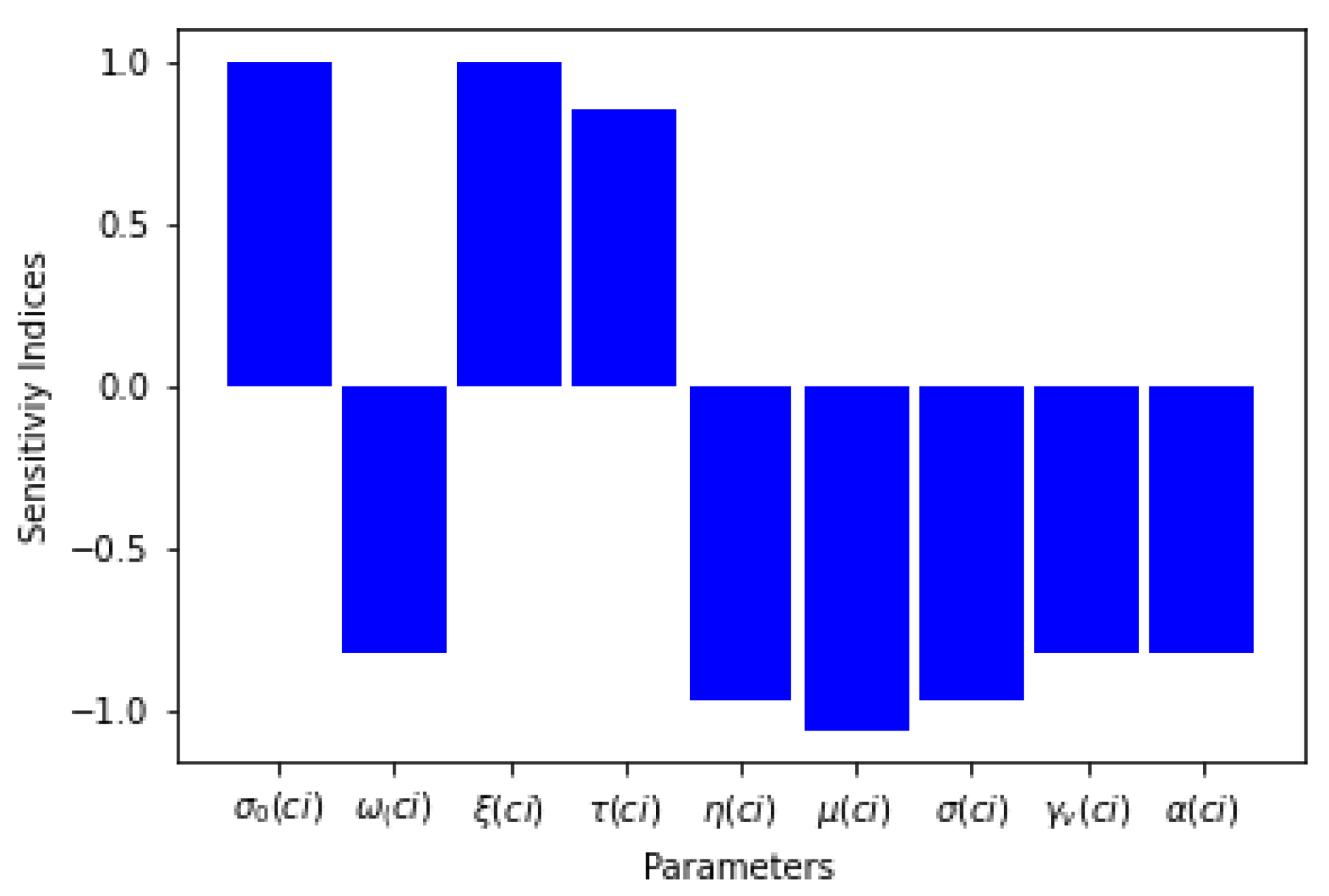
Six of the sensitivity indices are negative while the others are positive, as can be seen in Table 3. The sensitivity analysis of the basic reproduction number shows that there is a direct relationship between R 0 L ( t , c ) and the proportion of effective treatment of infectious humans for Lassa fever, the recruitment term of susceptible humans, and the progression rate of Lassa fever in the exposed human host while other parameters have an inverse relation with R 0 L ( t , c ) . Table 3 and Figure 1 present the sensitivity indices as they relate to R 0 L ( t , c ) .
What can be deduced from the sensitivity analysis of R 0 L ( t , c ) is that, if the rates of the proportions of effective treatment, diagnostic for treatment, and the treatment rate are increased for the human populations exposed to and infected by Lassa fever disease, the threshold parameter R 0 L ( t , c ) will decrease, which means that the spread of the disease will be curtailed.

3.2.2. Sensitivity Analysis of Basic Reproduction Number, R 0 B ( t , a )

The sensitivity index of the basic reproduction number, R 0 B ( t , a ) with respect to parameter its parameters say P is given by:
S P R 0 B ( t , a ) = R 0 B ( t , a ) P · P R 0 B ( t , a )
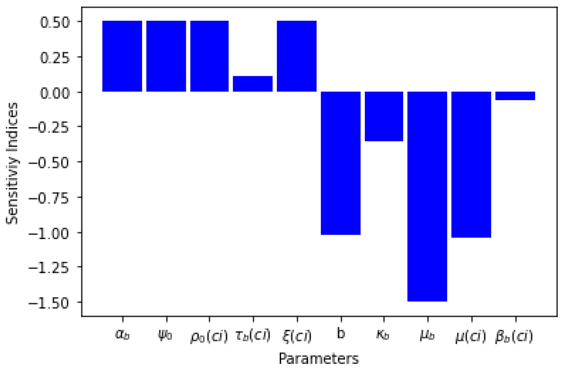
Five of the sensitivity indices are positive while other five are negative, as can be seen in Table 4. The sensitivity analysis of the basic reproduction number, R 0 B ( t , a ) shows that the bite rate, seasonal variation of black fly and treatment of infectious human for onchocerciasis have an inverse relation with R 0 B ( t , a ) . Table 4 and Figure 2 present the sensitivity indices as they relate to R 0 B ( t , a ) .
What can be deduced from the sensitivity analysis is that if the rate of treatment of infectious human for onchocerciasis is increased, the threshold parameter R 0 B ( t , a ) will decrease, which means the spread of the disease will be curtailed.
Treatment is critical in the treatment and management of onchocerciasis and Lassa fever. Treatment with the medicine ivermectin for onchocerciasis can efficiently destroy the microfilarial worms that cause the disease, limiting further transmission and lowering the risk of blindness. In addition to ivermectin, vector control strategies such as insecticide spraying can be used to limit the number of disease-carrying black flies. For Lassa fever, ribavirin is most effective when administered early in the course of the illness, which can significantly improve the patient outcomes. Additionally, supportive care, including fluid and electrolyte management, oxygen therapy, and the treatment of secondary infections, is essential for managing Lassa fever. The effective treatment of OLF can significantly reduce the burden of these diseases and improve the quality of life for the affected individuals. However, the treatment alone is not sufficient for controlling these diseases; comprehensive control strategies that include vector control and public health education are also essential.

3.3. Existence of Endemic Equilibrium

Using the basic reproduction number obtained from the model (1), we analyze the stability of the equilibrium point in the following result.
Theorem 2.
The OLF co-infection model (1) has no endemic equilibrium when R s 1 e ( c ) , R s 2 e ( c ) , R 0 B ( c ) ,   R b 1 e ( c ) , R b 2 e ( c ) < 1 and a unique endemic equilibrium exists when R s 1 e ( c ) , R s 2 e ( c ) , R 0 B ( c ) , R b 1 e ( c ) , R b 2 e ( c ) > 1 .
Proof. 
Let E e * * = ( N s s * * ( c i ) , N s e * * ( c i ) , N s i * * ( c i ) , N s r * * ( c i ) , N e s * * ( c i ) , N i s * * ( c i ) , N r s * * ( c i ) , S b * * , E b * * , I b * * , S r * * ( d j ) , E r * * ( d j ) , I r * * ( d j ) ) be a non-trivial equilibrium of the model (1). The steady state of the OLF co-infection model (1) are
N s s * * ( c ) = i = 0 L ζ ( c i ) ( R e b 2 2 ( c ) 1 ) μ ( c i ) R 0 B 2 ( c ) ( R e b 1 2 ( c ) 1 ) ,
N e s * * ( c ) = i = 0 L ζ ( c i ) ( γ b ( c i ) + μ ( c i ) ) ( μ ( c i ) + ϵ b ( c i ) β b ( c i ) ) ( R 0 B 2 ( c ) 1 ) τ b ( c i ) ϵ b ( c i ) β b ( c i ) R 0 B 2 ( c ) ( R b 1 e ( c ) 1 ) γ b ( c i ) ,
N i s * * ( c ) = i = 0 L ζ ( c i ) ( γ b ( c i ) + μ ( c i ) ) ( R 0 B 2 ( c ) 1 ) γ b ( c i ) R 0 B 2 ( c ) ( R b 1 e ( c ) 1 ) ,
N r s * * ( c ) = i = 0 L ζ ( c i ) ( R 0 B 2 ( c ) 1 ) R 0 B 2 ( c ) ( R e b 1 2 ( c ) 1 ) γ b ( c i ) ,
S b * * = i = 0 L ς ( c i ) ( 1 + κ cos ( 2 π t + T ) ) β b ( c i ) R 0 B 2 ( c ) ( R e b 1 2 ( c ) 1 ) γ b ( c i ) λ b ( γ b ( c i ) + μ ( c i ) ) ζ ( c i ) ( R 0 B 2 ( c ) 1 ) + R 0 B 2 ( c ) ( R e b 1 2 ( c ) 1 ) γ b ( c i ) B 0 ,
E b * * = i = 0 L ς b ϵ b ( c i ) β b ( c i ) λ b ( γ b ( c i ) + μ ( c i ) ) ζ ( c i ) ( R 0 B 2 ( c ) 1 ) R 0 B 2 ( c ) ( R e b 1 2 ( c ) 1 ) γ b ( c i ) ( μ b + α b ) ϵ b ( c i ) β b ( c i ) B 1 ,
I b * * = i = 0 L α b ϵ b ( c i ) β b ( c i ) ς b λ b ( γ b ( c i ) + μ ( c i ) ) ζ ( c i ) ( R 0 B 2 ( c ) 1 ) R 0 B 2 ( c ) ( R e b 1 2 ( c ) 1 ) μ b ( μ b + α b ) ϵ b ( c i ) β b ( c i ) B 1 ,
where
B 0 = ϵ b ( c i ) β b ( c i ) ( μ b + ξ b ς b ) and B 2 = λ b ( γ b ( c i ) + μ ( c i ) ) ζ ( c i ) ( R 0 B 2 ( c ) 1 ) + R 0 B 2 ( c ) ( R e b 1 2 ( c ) 1 ) γ b ( c i ) ϵ b ( c i ) β b ( c i ) μ b ,
R e b 1 2 ( c ) = i = 0 L ( μ ( c i ) μ b ( μ b + α b ) + α b λ B ς b ( 1 + κ b cos ( 2 π t + T ) ) θ b γ b ( c i ) α b λ B ς b ( 1 + κ b cos ( 2 π t + T ) ) τ b ( c i ) ϵ b ( c i ) β b ( c i ) ,
R e b 2 2 ( c ) = i = 0 L ( μ ( c i ) μ b ( μ b + α b ) R 0 B 2 ( c ) + α b λ B ς b ( 1 + κ b cos ( 2 π t + T ) ) ) θ b γ b ( c i ) α b λ B ς b ( 1 + κ b cos ( 2 π t + T ) ) τ b ( c i ) ϵ b ( c i ) β b ( c i ) ,
θ b = ( μ ( c i ) + τ b ( c i ) ) ( γ b ( c i ) + μ ( c i ) ) ( μ ( c i ) + ϵ b ( c i ) β b ( c i ) ) . Therefore,
I B * = N e s * + N i s * = i = 0 L ( γ b ( c i ) + μ ( c i ) ) ( μ ( c i ) + ϵ b ( c i ) β b ( c i ) ) ζ ( c i ) ( R 0 B 2 ( c ) 1 ) + θ k τ b ( c i ) ϵ b ( c i ) β b ( c i ) R 0 B 2 ( c ) γ b ( c i ) ( R e b 1 2 ( c ) 1 ) , where θ k = ζ ( c i ) ( γ b ( c i ) + μ ( c i ) ) ( R 0 B 2 ( c ) 1 ) τ b ( c i ) ϵ b ( c i ) β b ( c i )
For the Lassa fever class, it follows that:
N s s * * ( c ) = j = 0 T i = 0 L ζ ( c i ) μ ( c i ) R s 1 e ( c ) ( μ ( c i ) + γ 1 ( c i ) α ( c i ) + τ ( c i ) ) ( μ ( c i ) + η 1 ( c i ) σ ( c i ) ) λ a [ γ 1 ( c i ) α ( c i ) ( μ ( c i ) + η 1 ( c i ) σ ( c i ) ) + τ ( c i ) η 1 ( c i ) σ ( c i ) ] , N s e * * ( c ) = j = 0 T i = 0 L ( μ ( c i ) + η 1 ( c i ) σ ( c i ) ) ζ ( c i ) μ ( c i ) R s 1 e ( c ) γ 1 ( c i ) α ( c i ) ( μ ( c i ) + η 1 ( c i ) σ ( c i ) ) + τ ( c i ) η 1 ( c i ) σ ( c i ) , N s i * * ( c ) = i = 0 L j = 0 T τ ( c i ) μ ( c i ) ζ ( c i ) R s 1 e ( c ) γ 1 ( c i ) α ( c i ) ( μ ( c i ) + η 1 ( c i ) σ ( c i ) ) + τ ( c i ) η 1 ( c i ) σ ( c i ) , N s r * * ( c ) = i = 0 L j = 0 T ζ ( c i ) R s 1 e ( c i ) , S d * * ( e ) = j = 0 T Λ r ( d j ) ( 1 + ξ r cos ( 2 π t + T ) ) λ r R s 2 e ( c ) + μ r ( d j ) + δ r ( d j ) , E d * * ( e ) = j = 0 T λ r R s 2 e ( c ) Λ r ( d j ) ( 1 + ξ r cos ( 2 π t + T ) ) ( λ r R s 2 e ( c ) + μ r ( d j ) + δ r ( d j ) ) ( α r ( d j ) + μ r ( d j ) + δ r ( d j ) ) , I d * * ( e ) = α r ( d j ) Λ r ( d j ) ( 1 + ξ r cos ( 2 π t + T ) ) β 2 ( d j ) ( α r ( d j ) + μ r ( d j ) + δ r ( d j ) A d ( μ r ( d j ) + δ r ( d j ) ) ( α r ( d j ) + μ r ( d j ) + δ r ( d j ) ) β 2 ( d j ) w 2 ( d j ) = R s 2 e ( c )
where
R s 1 e ( c ) = i = 0 L j = 0 T λ a [ γ ( c i ) α ( c i ) ( μ ( c i ) + η 1 ( c i ) σ ( c i ) ) + τ ( c i ) η 1 ( c i ) σ ( c i ) ] ( μ ( c i ) + η 1 ( c i ) σ ( c i ) ) [ ( μ ( c i ) + γ 1 ( c i ) α ( c i ) + τ ( c i ) ) + μ ( c i ) λ a θ s ]
θ s = μ ( c i ) + γ 1 ( c i ) α ( c i ) , A d = Λ r ( d j ) ( 1 + ξ r cos ( 2 π t + T ) ) ( μ r ( d j ) + δ r ( d j ) )
Similarly,
I L * * = N s e * * ( c i ) + N s i * * ( c i ) = i = 0 L j = 0 T ( μ ( c i ) + η 1 ( c i ) σ ( c i ) ) μ ( c i ) R s 1 e ( c ) + τ ( c i ) μ ( c i ) R s 1 e ( c ) γ ( c i ) α ( c i ) ( μ ( c i ) + η 1 ( c i ) σ ( c i ) + τ ( c i ) η 1 ( c i ) σ ( c i ) ) .
The endemic state exists whenever R s 1 e ( c ) , R s 2 e ( c ) , R 0 B ( c ) , R b 1 e ( c ) , R b 2 e ( c ) > 1 . □

4. OLF Co-Infection Model Optimal Control

Into the model (1), we introduce preventative measures that are time-dependent v 1 ( t ) and the treatment v 2 ( t ) which employs the use of insecticide (or pesticide) v 3 ( t ) effort to curtail the transmission of OLF co-infection. The function 0 v 1 ( t ) 1 governs the measure regarding the utilization of face nets and long cloths for effective protection, as well as the use of rodent-proof containers, infection control measures such as complete equipment sterilization, improved home hygiene, and strict barrier nursing such as masks, gloves, gowns, and goggles to prevent human-to-human contact. The function 0 v 2 ( t ) 1 is the control in the treatment of OLF. The insecticide used for the black fly net is lethal to the black flies and other insects and repels the black flies, thus reducing the number that attempt to feed on people in the sleeping areas with the nets. Hence, the transition dynamics are given by
d N s s t , c i d t = ζ c i i = 0 L j = 0 T λ a + λ b N s s t , c i 1 v 1 i = 0 L λ B N s s t , c i I b 1 v 1 μ c i N s s t , c i + γ b c i N r s t , c i d N s e t , c i d t = i = 0 L j = 0 T λ a + λ b N s s t , c i 1 v 1 i = 0 L ϑ b c i λ B N s e t , c i I b 1 v 1 μ c i + γ 1 c i α c i v 2 + τ c i N s e t , c i d N s i t , c i d t = i = 0 L τ c i N S e t , c i i = 0 L ϑ b c i λ B N S i t , c i I b 1 v 1 μ c i + η 1 c i σ c i v 2 N s i t , c i d N s r t , c i d t = i = 0 L γ 1 c i α c i v 2 N s e t , c i + η 1 c i σ c i v 2 N s i t , c i μ c i N s r t , c i d N e s t , c i d t = i = 0 L λ B N s s t , c i I b 1 v 1 i = 0 L j = 0 T ϑ r c i λ a + λ b N e s t , c i 1 v 1 μ c i + τ b c i N e s t , c i d N i s t , c i d t = i = 0 L τ b c i N e S t , c i i = 0 L j = 0 T ϑ r c i λ a + λ b N i s t , c i 1 v 1 μ c i + ϵ b c i β b c i v 2 N i s t , c i d N r s t , c i d t = i = 0 L ϵ b c i β b c i v 2 N i s t , c i γ b c i + μ c i N r s t , c i d N r r t , c i d t = i = 0 L ϑ b c i λ B N s e t , c i + N s i t , c i 1 v 1 I b μ c i N r r t , c i + i = 0 L j = 0 T ϑ r c i λ a + λ b N e S t , c i + N i S t , c i 1 v 1 d S r t , d j d t = Λ r d j 1 + ξ r cos ( 2 π t + T ) j = 0 T λ r S r t , d j I r t , d j μ r d j + δ r d j + 1 v 3 S r t , d j d E r t , d j d t = j = 0 T λ r S r t , d j I r t , d j α r d j + μ r d j + δ r d j + 1 v 3 E r t , d j d I r t , d j d t = j = 0 T α r d j E r t , d j μ r d j + δ r d j + 1 v 3 I r t , d j d S b d t = ς b Λ r d j 1 + κ b cos ( 2 π t + T ) λ b S b N i s t , c i 1 v 1 μ b + 1 v 3 S b d E b d t = λ b S b N i S t , c i 1 v 1 μ b + α b + 1 v 3 E b d I b d t = α b E b μ b + 1 v 3 I b

4.1. Global Stability Analysis

This is achieved for both the disease-free and endemic equilibria for the special case with no loss of immunity acquired by the recovered individuals and no reduction in the black fly and rodent groups.
Theorem 3.
The disease-free equilibrium point ϵ 0 of the model (13) is globally asymptotically stable in Ω if R 0 L ( x ) 1 and R 0 B ( x ) 1 .
Proof. 
The Lyapunov function is given by
P = μ ( c i ) ( η 1 ( c i ) σ ( c i ) v 2 + μ ( c i ) ) N s e ( t , c i ) + σ 0 ( 1 + w 1 ( c i ) cos ( 2 π t + T ) ) ζ ( c i ) τ ( c i ) N s i ( t , c i ) τ ( c i ) + μ ( c i ) N h ( t , c i ) ( ϵ b ( c i ) β b ( c i ) v 2 + μ ( c i ) ) μ b ( α b + μ b ) N e s ( t , c i ) + τ b ( c i ) c 0 ( c i ) ( 1 + b cos ( 2 π t + T ) ) ζ ( c i ) α b ς b ( 1 + κ b cos ( 2 π t + T ) ) ϕ 0 N i s ( t , c i ) τ b + σ 0 ( 1 + w 1 ( c i ) cos ( 2 π t + T ) ) ζ ( c i ) τ ( c i ) I r ( t , d j ) μ r ( d j ) μ ( c i ) ( η 1 ( c i ) σ ( c i ) v 2 + μ ( c i ) ) ( γ 1 ( c i ) α ( c i ) v 2 + τ ( c i ) + μ ( c i ) ) + τ b ( c i ) c 0 ( c i ) ( 1 + b cos ( 2 π t + T ) ) ζ ( c i ) α b ς b ( 1 + κ b cos ( 2 π t + T ) ) ϕ 0 I b ( t ) μ ( c i ) N h ( t , c i ) ( τ b ( c i ) + μ ( c i ) ) ( ϵ b ( c i ) β b ( c i ) v 2 + μ ( c i ) ) μ b ( α b + μ b ) + σ 0 ( 1 + w 1 ( c i ) cos ( 2 π t + T ) ) ζ ( c i ) τ ( c i ) E r ( t , d j ) ( α r ( d j ) + μ r ( d j ) + δ r ( d j ) ) ( η 1 ( c i ) σ ( c i ) v 2 + μ ( c i ) ) ( γ 1 ( c i ) α ( c i ) v 2 + τ ( c i ) + μ ( c i ) ) + τ b ( c i ) c 0 ( c i ) ( 1 + b cos ( 2 π t + T ) ) ζ ( c i ) α b ς b ( 1 + κ b cos ( 2 π t + T ) ) ϕ 0 E b ( t ) μ ( c i ) N h ( t , c i ) ( τ b ( c i ) + μ ( c i ) ) ( ϵ b ( c i ) β b ( c i ) v 2 + μ ( c i ) ) μ b ( α b + μ b )
The time derivative of P yields
P ˙ = μ ( c i ) ( η 1 ( c i ) σ ( c i ) v 2 + μ ( c i ) ) i = 0 L j = 0 T ( λ a + λ b ) N s s ( t , c i ) ( 1 v 1 ) μ ( c i ) ( η 1 ( c i ) σ ( c i ) v 2 + μ ( c i ) ) j = 0 T ϑ b ( c i ) λ B N s e ( t , c i ) I b ( 1 v 1 ) μ ( c i ) ( η 1 ( c i ) σ ( c i ) v 2 + μ ( c i ) ) ( μ ( c i ) + γ 1 ( c i ) α ( c i ) v 2 + τ ( c i ) ) N s e ( t , c i ) + σ 0 ( 1 + w 1 ( c i ) cos ( 2 π t + T ) ) ζ ( c i ) τ ( c i ) τ ( c i ) i = 0 L τ ( c i ) i = 0 L ϑ b ( c i ) λ B N s i ( t , c i ) I b ( 1 v 1 ) σ 0 ( 1 + w 1 ( c i ) cos ( 2 π t + T ) ) ζ ( c i ) τ ( c i ) τ ( c i ) μ ( c i ) + η 1 ( c i ) σ ( c i ) v 2 N s i ( t , c i ) + μ ( c i ) N h ( t , c i ) ( ϵ b ( c i ) β b ( c i ) v 2 + μ ( c i ) ) ( α b + μ b ) λ B N s i ( t , c i ) I b ( 1 v 1 ) μ ( c i ) N h ( t , c i ) ( ϵ b ( c i ) β b ( c i ) v 2 + μ ( c i ) ) ( α b + μ b ) i = 0 L j = 0 T ϑ r ( d j ) ( λ a + λ b ) N e s ( t , c i ) ( 1 v 1 ) μ ( c i ) N h ( t , c i ) ( ϵ b ( c i ) β b ( c i ) v 2 + μ ( c i ) ) ( α b + μ b ) ( μ ( c i ) + τ b ( c i ) N e s ( t , c i ) ) + τ b ( c i ) c 0 ( c i ) c 0 ( c i ) ( 1 + b cos ( 2 π t + T ) ) ζ ( c i ) ς b α b ϕ 0 τ b ( c i ) × i = 0 L τ b ( c i ) N e s ( t , c i ) i = 0 L j = 0 T ϑ r ( d j ) ( λ a + λ b ) N i s ( t , c i ) ( 1 v 1 ) τ b ( c i ) c 0 ( c i ) ( 1 + b cos ( 2 π t + T ) ) ζ ( c i ) ς b α b ϕ 0 τ b ( c i ) μ ( c i ) + ϵ b ( c i ) β b ( c i ) v 2 N i s ( t , c i ) + σ 0 ( c i ) ( 1 + w 1 ( c i ) cos ( 2 π t + T ) ) ζ ( c i ) τ ( c i ) μ r ( d j ) μ ( c i ) ( η 1 ( c i ) σ ( c i ) v 2 + μ ( c i ) ) ( μ ( c i ) + γ 1 ( c i ) α ( c i ) v 2 + τ ( c i ) ) × j = 0 T α r ( d j ) E r ( t , d j ) ( μ ( d j ) + δ r ( d j ) ) I r ( t , d j ) + c 0 ( c i ) c 0 ( c i ) ( 1 + b cos ( 2 π t + T ) ) τ b ( c i ) ζ ( c i ) ς b ( 1 + κ b cos ( 2 π t + T ) ) α b ϕ 0 μ ( c i ) N h ( t , c i ) ( τ b ( c i ) + μ ( c i ) ) ( ϵ b ( c i ) β b ( c i ) v 2 + μ ( c i ) ) μ b 2 ( α b + μ b ) ( α b E b + μ b I b )
+ σ 0 ( c i ) ( 1 + w 1 ( c i ) cos ( 2 π t + T ) ) ζ ( c i ) τ ( c i ) ( α r ( d j ) + μ r ( d j ) + δ r ( d j ) ) ( η 1 ( c i ) σ ( c i ) v 2 + μ ( c i ) ) ( γ 1 ( c i ) α ( c i ) v 2 + τ ( c i ) μ ( c i ) ) × j = 0 T ( λ r ( t ) S r ( t , d j ) I r ( t , d j ) ( α r ( d j ) + μ r ( d j ) + δ r ( d j ) ) E r ( t , d j ) + τ b ( c i ) c 0 ( c i ) ( 1 + b cos ( 2 π t + T ) ) ζ ( c i ) ς b ( 1 + κ b cos ( 2 π t + T ) ) α b ϕ 0 λ h m μ ( c i ) N h ( t , c i ) ( τ b ( c i ) + μ ( c i ) ) ( ϵ b ( c i ) β b ( c i ) v 2 + μ ( c i ) ) μ b ( α b + μ b )
where
λ h b = λ b S b N i s ( t , c i ) ( 1 v 1 ) ( μ b + α b ) E b
Further simplification gives
P ˙ < μ ( c i ) ( η 1 ( c i ) σ ( c i ) v 2 + μ ( c i ) ) ( μ ( c i ) + γ 1 ( c i ) α ( c i ) v 2 + τ ( c i ) ) N s e ( t , c i ) + σ 0 ( 1 + w 1 ( c i ) cos ( 2 π t + T ) ) ζ ( c i ) τ ( c i ) N s e ( t , c i ) σ 0 ( 1 + w 1 ( c i ) cos ( 2 π t + T ) ) ζ ( c i ) τ ( c i ) ( η 1 ( c i ) σ ( c i ) v 2 ) N s i ( t , c i ) τ ( c i ) μ ( c i ) N h ( t , c i ) ( ϵ b ( c i ) β b ( c i ) v 2 + μ ( c i ) ) μ b ( α b + μ b ) ( μ ( c i ) + τ b ( c i ) ) N e s ( t , c i ) + τ b ( c i ) c 0 ( c i ) ( 1 + b cos ( 2 π t + T ) ) ϵ b ( c i ) β b ( c i ) v 2 ζ ( c i ) α b ϕ 0 N e s ( t , c i ) τ b ( c i ) c 0 ( c i ) ( 1 + b cos ( 2 π t + T ) ) ς b ( 1 + κ b ( 2 π t + T ) ) ζ ( c i ) α b ϕ 0 ( μ ( c i ) + ϵ b ( c i ) β b ( c i ) v 2 ) N i s ( t , c i ) τ b ( c i ) τ b ( c i ) c 0 ( c i ) ( 1 + b cos ( 2 π t + T ) ) ς b ( 1 + κ b ( 2 π t + T ) ) ζ ( c i ) α b ϕ 0 I b ( t ) μ ( c i ) N h ( t , c i ) ( μ ( c i ) + τ b ( c i ) ) ( ϵ b ( c i ) β b ( c i ) v 2 + μ ( c i ) ) μ b ( α b + μ b )
Equation (15) becomes
P ˙ < σ 0 w 1 ( c i ) ζ ( c i ) τ ( c i ) ( R 0 L ( x ) 1 ) N s e ( t , c i ) μ ( c i ) ( γ 1 ( c i ) α ( c i ) v 2 + τ ( c i ) + μ ( c i ) ) ( η 1 ( c i ) σ ( c i ) v 2 + μ ( c i ) ) 2 R 0 L ( x ) N s i ( t , c i ) τ ( c i ) + μ ( c i ) N h ( t , c i ) ( τ b ( c i ) + μ ( c i ) ) ( ϵ b ( c i ) β b ( c i ) v 2 + μ ( c i ) ) μ b ( α b + μ b ) ( R 0 B 2 ( x ) 1 ) N e s ( t , c i ) ( ϵ b ( c i ) β b ( c i ) v 2 + μ ( c i ) ) 2 μ ( c i ) N h ( t , c i ) ( τ b ( c i ) + μ ( c i ) ) μ b ( α b + μ b ) R 0 B 2 ( x ) τ b ( c i ) R 0 B 2 ( x ) I b ( t )
P ˙ < 0 if R 0 L ( x ) 1 and R 0 B ( x ) 1 .
The maximum invariant set: { ( N s s ( t , c i ) ,   N s e ( t , c i ) ,   N s i ( t , c i ) ,   N s r ( t , c i ) ,   N e s ( t , c i ) ,   N i s ( t , c i ) , N r s ( t , c i ) ,   N r r ( t , c i ) ,   S r ,   E r ,   I r ,   S b ,   E b ,   I b ) Ω : P ˙ = 0 } is the singleton ϵ 0 . In this set, N h ( t , c i ) Λ ( c i ) μ ( c i ) , N r ( t , d j ) Λ r ( d j ) ( 1 + ξ r cos ( 2 π t + T ) ) μ r ( d j ) + δ ( d j ) , and N b ( t ) ς b ( 1 + ξ r cos ( 2 π t + T ) ) μ b as t + . This shows that all solutions approach the disease-free stationary state. Thus, when R 0 B ( x ) , R 0 L ( x ) 1 both diseases will be eliminated from the system. If R 0 M ( x ) , R 0 L ( x ) > 1 , then P ˙ may be > 0 for N s e = N s i = N e s = N i s = I r = I b close to the disease-free state except for N s e = N s i = N e s = N i s = I r = I b = 0 . Thus, the disease-free state is globally asymptotically stable when R 0 B 2 ( x ) , R 0 L ( x ) 1 .
The nonlinear Lyapunov function of the Goh–Volterra type is used for the endemic equilibrium. See, for instance, [11] for the application of this Lyapunov function. □
Theorem 4.
The unique endemic equilibrium, E e , of the model (15) is globally asymptotically stable if R 0 B ( x ) > 1 , R 0 L ( x ) > 1 and 0 v 1 1 .
Proof. 
Let R 0 L ( x ) , R 0 B ( x ) > 1 and 0 v 1 1 so that a unique endemic equilibrium exists and consider the following nonlinear Lyapunov function defined by
N = N s s ( t , c i ) N s s * * ( c i ) N s s * * ( c i ) ln N s s ( t , c i ) N s s * * ( c i ) + N s e ( t , c i ) N s e * * ( c i ) N s e * * ( c i ) ln N s e ( t , c i ) N s e * * ( c i ) + N e s ( t , c i ) N e s * * ( c i ) N e s * * ( c i ) ln N e s ( t , c i ) N e s * * ( c i ) + μ ( c i ) + γ 1 ( c i ) α ( c i ) v 2 + τ ( c i ) τ ( c i ) N s i ( t , c i ) N s i * * ( c i ) N s i * * ( c i ) ln N s i ( t , c i ) N s i * * ( c i ) + μ ( c i ) + τ b ( c i ) τ b ( c i ) N i s ( t , c i ) N i s * * ( c i ) N i s * * ( c i ) ln N s i ( t , c i ) N i s * * ( c i ) + S r ( t , d j ) S r * * ( d j ) S r * * ( d j ) ln S r ( t , d j ) S r * * ( d j ) + E r ( t , d j ) E r * * ( d j ) E r * * ( d j ) ln E r ( t , d j ) E r * * ( d j ) + μ r ( d j ) + α r ( d j ) + δ r ( d j ) α ( d j ) I r ( t , d j ) I r * * ( d j ) I r * * ( d j ) ln I r ( t , d j ) I r * * ( d j ) + S b S b * * S b * * ln S b S b * * + E b E b * * E b * * ln E b E b * * + α b + μ b α b I b I b * * I b * * ln I b I b * *
with the Lyapunov time-derivative obtained as
N ˙ = N ˙ s s ( t , c i ) N s s * * ( c i ) N s s ( t , c i ) N ˙ s s ( t , c i ) + N ˙ s e ( t , c i ) N s e * * ( c i ) N s e ( t , c i ) N ˙ s e ( t , c i ) + N ˙ e s ( t , c i ) N e s * * ( c i ) N e s ( t , c i ) N ˙ e s ( t , c i ) + μ ( c i ) + γ 1 ( c i ) α ( c i ) v 2 + τ ( c i ) τ ( c i ) N ˙ s i ( t , c i ) N s i * * ( c i ) N s i ( t , c i ) N ˙ s i ( t , c i ) + μ ( c i ) + τ b ( c i ) τ b ( c i ) N ˙ i s ( t , c i ) N s i * * ( c i ) N i s ( t , c i ) N ˙ i s ( t , c i ) + S ˙ r ( t , d j ) S r * * ( d j ) S r ( t , d j ) S ˙ r ( t , d j ) + E ˙ r ( t , d j ) E r * * ( d j ) E r ( t , d j ) E ˙ r ( t , d j ) + μ r ( d j ) + α r ( d j ) + δ r ( d j ) α ( d j ) I ˙ r ( t , d j ) I r * * ( d j ) I r ( t , d j ) I ˙ r ( t , d j ) + S ˙ b S b * * S b S ˙ b + E ˙ b E b * * E b E ˙ b + α b + μ b α b I ˙ b I b * * I b I ˙ b
Using the appropriate equations of the model (15) in (18) further gives
N ˙ = i = 0 L ζ ( c i ) 1 + N s s * * ( c i ) N s s ( t , c i ) i = 0 L μ ( c i ) N s s ( t , c i ) 1 + N s s * * ( c i ) N s s ( t , c i ) + i = 0 L j = 0 T ( λ a + λ b ) N s s * * ( c i ) ( 1 v 1 ( t ) ) + i = 0 L λ B N s s * * ( c i ) I b ( 1 v 1 ( t ) ) i = 0 L j = 0 T ( λ a + λ b ) N s s ( t , c i ) N s e * * ( c i ) ( 1 v 1 ( t ) ) N s e ( t , c i ) + ( μ ( c i ) + γ 1 ( c i ) α ( c i ) v 2 ( t ) + τ ( c i ) ) N s e * * ( c i ) ) i = 0 L λ B N s s ( t , c i ) N e s * * ( c i ) I b ( 1 v 1 ( t ) ) N e s ( t , c i ) + ( μ ( c i ) + τ b ( c i ) ) N e s * * ( c i ) i = 0 L ( μ ( c i ) + γ 1 ( c i ) α ( c i ) v 2 ( t ) + τ ( c i ) ) ϑ b ( c i ) λ B N s i ( t , c i ) I b ( 1 v 1 ( t ) ) τ ( c i )
( μ ( c i ) + γ 1 ( c i ) α ( c i ) v 2 ( t ) + τ ( c i ) ) ( μ ( c i ) + η 1 ( c i ) σ ( c i ) v 2 ( t ) ) N s i ( t , c i ) τ ( c i ) i = 0 L ( μ ( c i ) + γ 1 ( c i ) α ( c i ) v 2 ( t ) + τ ( c i ) ) N s i * * ( c i ) N s e ( t , c i ) N s i ( t , c i ) + i = 0 L ϑ b ( c i ) λ B N s i * * ( c i ) I b ( t ) ( 1 v 1 ( t ) ) ( μ ( c i ) + γ 1 ( c i ) α ( c i ) v 2 ( t ) + τ ( c i ) ) τ ( c i ) + ( μ ( c i ) + γ 1 ( c i ) α ( c i ) v 2 ( t ) + τ ( c i ) ) N s i * * ( c i ) ( μ ( c i ) + η 1 ( c i ) σ ( c i ) v 2 ( t ) ) τ ( c i ) i = 0 L j = 0 T ϑ r ( c i ) ( λ a + λ b ) N i s ( t , c i ) ( μ ( c i ) + τ b ( c i ) ) ( 1 v 1 ( t ) ) τ b ( c i ) ( μ ( c i ) + ϵ b ( c i ) β b ( c i ) v 2 ( t ) ) ( μ ( c i ) + τ b ( c i ) ) N i s ( t , c i ) τ b ( c i ) i = 0 L ( μ ( c i ) + τ b ( c i ) ) N i s * * ( c i ) N e s ( t , c i ) N i s ( t , c i ) i = 0 L j = 0 T ϑ ( c i ) ( λ a + λ b ) N i s * * ( c i ) ( 1 v 1 ( t ) ) ( μ ( c i ) + τ b ( c i ) ) τ b ( c i ) + ( μ ( c i ) + ϵ b ( c i ) β b ( c i ) v 2 ( t ) ) N i s * * ( c i ) ( μ ( c i ) + τ b ( c i ) ) τ b ( c i ) + j = 0 T Λ r ( d j ) ( 1 + ξ r cos ( 2 π t + T ) ) 1 + S d * * ( c i ) S r ( t , d j ) j = 0 T ( μ r ( d j ) + δ ( d j ) ) S r ( t , d j ) 1 + S d * * ( c i ) S r ( t , d j ) + j = 0 T λ r ( t ) S d * * ( d j ) I r ( t , d j ) ( 1 v 3 ( t ) ) j = 0 T λ r ( t ) S r ( t , d j ) I r ( t , d j ) E d * * ( d j ) ( 1 v 3 ( t ) ) E r ( t , d j ) + ( α r ( d j ) + μ r ( d j ) + δ r ( d j ) ) E d * * ( d j ) ) ( α r ( d j ) + μ r ( d j ) + δ r ( d j ) ) ( μ r ( d j ) + δ r ( d j ) ) I r ( t , d j ) α r ( d j ) ( α r ( d j ) + μ r ( d j ) + δ r ( d j ) ) I d * * ( d j ) E r ( t , d j ) I r ( t , d j ) + ( α r ( d j ) + μ r ( d j ) + δ r ( d j ) ) I d * * ( d j ) ( μ r ( d j ) + δ r ( d j ) ) α r ( d j ) ς b ( 1 + ξ b cos ( 2 π t + T ) ) 1 + S b * * S b μ b S b 1 + S b * * S b ( α b + μ b ) I b * * E b I b + μ b ( α b + μ b ) I b α b + ( α b + μ b ) I b * * α b + λ b S b * * N i s ( t , c i ) ( 1 v 1 ( t ) ) λ b S b N i s ( t , c i ) ( 1 v 1 ( t ) ) E b * * E b + ( μ b + α b ) E b * * .
At the endemic equilibrium, it is seen from Equation (15) that
μ ( c i ) + γ ( c i ) α ( c i ) + τ ( c i ) = ( λ a * * + λ b * * ) N s s * * ( c i ) ϑ ( c i ) λ b N s e * * ( c i ) I b * * N s e * * ( c i ) μ ( c i ) + η 1 ( c i ) σ ( c i ) = τ ( c i ) N s e * * ( c i ) ϑ b ( c i ) λ B N s i * * ( c i ) I b * * N s i * * ( c i ) μ ( c i ) + τ b ( c i ) = λ B * N s s * * ( c i ) I b * * ϑ r ( c i ) ( λ a * * + λ b * * ) N e s * * ( c i ) N e s * * ( c i ) μ ( c i ) + ϵ b ( c i ) β b ( c i ) = ϑ r ( c i ) ( λ a * * + λ b * * ) N i s * * ( c i ) + τ b ( c i ) N e s * * ( c i ) N i s * * ( c i ) α r ( d j ) + μ r ( d j ) + δ r ( d j ) = λ d * * S d * * ( d j ) I d * * ( d j ) E d * * ( d j ) μ r ( d j ) + δ r ( d j ) = α r ( d j ) E d * * ( d j ) I d * * ( d j ) μ b + α b = λ b * * S b * * N i s * * ( c i ) E b * * Λ r ( c i ) ( 1 + ξ r cos ( 2 π t + T ) ) = λ d * * S d * * ( d j ) I d * * ( d j ) + ( μ r ( d j ) + δ r ( d j ) ) S d * * ( d j ) ζ ( c i ) = ( λ a * * + λ b * * ) N s s * * ( c i ) + λ B * * N s s * * ( c i ) I b * * + μ ( c i ) N s s * * ( c i ) ς b ( 1 + κ b cos ( 2 π t + T ) ) = λ b * * S b * * N i s * * ( c i ) + μ b S b * * .
μ b = α b E b * * I b * *
Using Equation (20) in Equation (19) and then systematically adding and subtracting the following i = 0 L j = 0 T ( λ a * * + λ b * * ) N s s * * ( c i ) ( 1 v 1 ) , λ B * * N s s * * ( c i ) I b * * ( 1 v 1 )   i = 0 L j = 0 T ( λ a * * + λ b * * ) N s s * * ( c i ) ( 1 v 1 ) I h ( t , c i ) f 2 ( N h * * ) I h * * ( c i ) f ( N h ) , λ B * * N s s * * I h ( t , c i ) f 2 ( N h * * ) ( 1 v 1 ) I h * * ( c i ) f ( N h ) , λ d * * S d * * ( d j ) I d * * ( d j ) ( 1 v 3 ) , λ d * * S d * * ( d j ) I r ( t , c i ) ( 1 v 3 ) f 2 ( N d * * I d * * ( d j ) f ( N r ) λ b * * S b * * N i s * * ( c i ) ( 1 v 1 ) , λ b * * S b * * N i s ( t , c i ) ( 1 v 1 ) f 2 ( N b * * ) N i s * * ( c i ) f ( N b ) one gets
N ˙ = i = 0 L μ ( c i ) N s s * * ( c i ) 2 N s s * * ( c i ) N s s ( t , c i ) N s s ( t , c i ) N s s * * ( c i ) + i = 0 L j = 0 T ( λ a + λ b ) N s s * * ( c i ) ( 1 v 1 ) f ( N h * * ) × 4 N s s * * ( c i ) N s s ( t , c i ) N s e * * ( c i ) N s s ( t , c i ) N s s * * ( c i ) N s e ( t , c i ) N s i * * ( c i ) N s e ( t , c i ) N s i ( t , c i ) I h ( t , c i ) f ( N h * * ) I h * * ( c i ) f ( N h ) i = 0 L j = 0 T N s s * * ( c i ) ( 1 v 1 ) f ( N h * * ) × 2 I h ( t , c i ) f ( N h * * I h * * ( c i ) f ( N h ) f ( N h ) f ( N h * * ) i = 0 L c 0 ( 1 + b cos ( 2 π t + T ) ) ( c i ) N s s * * ( c i ) I b * * ( 1 v 1 ) f ( N h * * ) × 2 I h ( t , c i ) f ( N h * * I h * * ( c i ) f ( N h ) f ( N h ) f ( N h * * ) i = 0 L c 0 ( 1 + b cos ( 2 π t + T ) ) N s s * * ( c i ) I b * * ( 1 v 1 ) f ( N h * * ) × 4 N s s * * ( c i ) N s s ( t , c i ) N e s * * ( c i ) I b N s s ( t , c i ) N s s * * ( c i ) N e s ( t , c i ) I b * * N i s * * ( c i ) N e s ( t , c i ) I b N i s ( t , c i ) I b * * I h ( t , c i ) f ( N h * * ) I h * * ( c i ) f ( N h ) i = 0 L ϑ b ( a 1 ) c 0 ( c i ) ( 1 + b cos ( 2 π t + T ) ) N s e * * ( c i ) I b * * ( 1 v 1 ) f ( N h * * ) 1 N s i * * ( c i ) N s e ( t , c i ) N s i ( t , c i ) i = 0 L j = 0 T ϑ r ( c i ) ( λ a * * + λ b * * ) N e s * * ( c i ) ( 1 v 1 ) f ( N h * * ) 1 N i s * * ( c i ) N e s ( t , c i ) N i s ( t , c i ) + j = 0 T ( μ r ( d j ) + δ r ( d j ) ) S d * * ( d j ) 2 S d * * ( d j ) S r ( t , c i ) S r ( t , c i ) S d * * ( d j ) + j = 0 T λ r S d * * ( d j ) I d * * ( d j ) ( 1 v 3 ) f ( N d * * ) × 4 S d * * ( d j ) S r ( t , d j ) I d * * ( d j ) E r ( t , d j ) E d * * ( d j ) I r ( t , d j ) S r ( t , d j ) I r ( t , d j ) E d * * ( d j ) S d * * ( d j ) I d * * ( d j ) E r ( t , d j ) I r ( t , d j ) f ( N d * * ) I d * * ( d j ) f ( N r ) j = 0 T λ r ( t ) S d * * ( d j ) I d * * ( d j ) ( 1 v 3 ) f ( N d * * ) 2 I r ( t , d j ) f ( N d * * ) f ( N r ) ( I d * * ( d j ) ) 2 f ( N r ) I r ( t , d j ) I d * * ( d j ) f ( N d * * )
+ μ b S b * * 2 S b * * S b S b S b * * + λ b S b * * N i s * * ( c i ) ( 1 v 1 ) f ( N b * * ) × 4 S b * * S b I b * * E b E b * * I b S b N i s ( t , c i ) E b * * S b * * N s i * * ( c i ) E b I b f ( N b * * ) I b * * f ( N b ) λ b S b * * N i s * * ( c i ) ( 1 v 1 ) f ( N b * * ) 2 N i s ( t , c i ) f ( N b * * ) N i s * * ( c i ) f ( N b ) N i s ( t , c i ) f ( N b * * ( N i s * * ( c i ) ) 2 f ( N b )
Further simplification gives
N ˙ = A 1 A 2 i = 0 L j = 0 T ( λ a + λ b ) N s s * * ( c i ) ( 1 v 1 ) f ( N h * * ) × 2 I h ( t , c i ) f ( N h * * ) I h * * ( c i ) f ( N h ) f ( N h ) f ( N h * * i = 0 L λ b N s s * * ( c i ) I b * * ( 1 v 1 ) f ( N h * * ) × 2 I h ( t , c i ) f ( N h * * ) I h * * ( c i ) f ( N h ) f ( N h ) f ( N h * * A 3 i = 0 L ϑ b ( c i ) λ b N s e * * ( c i ) I b * * ( 1 v 1 ) f ( N h * * ) × 1 N s i * * ( c i ) N s e ( t , c i ) N s i ( t , c i ) N s e * * ( c i ) i = 0 L j = 0 T ϑ ( c i ) ( λ a + λ b ) × N e s * * ( c i ) ( 1 v 1 ) f ( N h * * ) 1 N i s * * ( c i ) N e s ( t , c i ) N i s ( t , c i ) N e s * * ( c i ) A 4 A 5 j = 0 T λ r S d * * ( d j ) I d * * ( d j ) ( 1 v 1 ) f ( N d * * ) 2 I r ( t , d j ) f ( N d * * ) f ( N r ) ( I d * * ( d j ) ) 2 f ( N r ) I r ( t , d j ) I d * * ( d j ) f ( N d * * ) A 6 A 7 λ b S b * * N i s * * ( c i ) ( 1 v 1 ) f ( N b * * ) 2 N i s ( t , c i ) f ( N b ) N i s * * ( c i ) f ( N b ) N i s ( t , c i ) f ( N b * * ( N i s * * ( c i ) ) 2 f ( N b )
where
A 1 = i = 0 L μ ( c i ) N s s * * ( c i ) 2 N s s * * ( c i ) N s s ( t , c i ) N s s ( t , c i ) N s s * * ( c i )
A 2 = i = 0 L j = 0 T ( λ a + λ b ) N s s * * ( c i ) ( 1 v 1 ) f ( N h * * ) × 4 N s s * * ( c i ) N s s ( t , c i ) N e s * * ( c i ) N s s ( t , c i ) N s s * * ( c i ) N s e ( t , c i ) N i s * * ( c i ) N s e ( t , c i ) N s i ( t , c i ) I h ( t , c i ) f ( N h * * ) I h * * ( c i ) f ( N h )
A 3 = i = 0 L λ b ( t ) N s s * * ( c i ) I b * * ( 1 v 1 ) f ( N h * * ) × 4 N s s * * ( c i ) N s s ( t , c i ) N e s * * ( c i ) I b N s s ( t , c i ) N s s * * ( c i ) N e s ( t , c i ) I b * * N i s * * ( c i ) N e s ( t , c i ) I b N i s ( t , c i ) I b * * I h ( t , c i ) f ( N h * * ) I h * * ( c i ) f ( N h )
A 4 = j = 0 T ( μ r ( d j ) + δ r ( d j ) ) S d * * ( d j ) 2 S d * * ( d j ) S r ( t , c i ) S r ( t , c i ) S d * * ( d j )
A 5 = j = 0 T λ r S d * * ( d j ) I d * * ( d j ) ( 1 v 3 ) f ( N d * * ) × 4 S d * * ( d j ) S r ( t , d j ) I d * * ( d j ) E r ( t , d j ) E d * * ( d j ) I r ( t , d j ) S r ( t , d j ) I r ( t , d j ) E d * * ( d j ) S d * * ( d j ) I d * * ( d j ) E r ( t , d j ) I r ( t , d j ) f ( N d * * ) I d * * ( d j ) f ( N r )
A 6 = μ b S b * * 2 S b * * S b S b S b * *
A 7 = λ b S b * * N i s * * ( c i ) ( 1 v 1 ) f ( N b * * ) × 4 S b * * S b I b * * E b E b * * I b S b N i s ( t , c i ) E b * * S b * * N s i * * ( c i ) E b I b f ( N b * * ) I b * * f ( N b )
We need to show that A 1 0 , A 2 0 , A 3 0 , A 4 0 , A 5 0 , A 6 0 , and A 7 0 . ( N s s * * ( c i ) ) 2 + ( N s s ( t , c i ) ) 2 2 N s s * * ( c i ) N s s ( t , c i ) 0 so that, N s s * * ( c i ) N s s ( t , c i ) + N s s ( t , c i ) N s s * * ( c i ) 2 0 . Hence, L 1 0 .
Furthermore, let x = N s s * * ( c i ) N s s ( t , c i ) , y = N e s * * ( c i ) f ( N h ) N s e ( t , c i ) f ( N h * * ) , z = N s i * * ( c i ) f ( N h * * ) N s i ( t , c i ) f ( N h * * ) .
Then, N s s * * ( c i ) N s s ( t , c i ) + N s e * * ( c i ) N s s ( t , c i ) N s s * * ( c i ) N s e ( t , c i ) + N s i * * ( c i ) N s e ( t , c i ) N s i ( t , c i ) + I h ( t , c i ) f ( N h * * ) I h * * ( c i ) f ( N h ) 4 can be written as
f ( x , y , z ) = x + y x + z y + 1 z 4
It suffices to show that f ( x , y , z ) 0 . Since f x = f y = f z = 0 gives rise to x = y = z and that f x x > 0 , f y y > 0 , f z z > 0 , one can see that the minimum of f ( x , y , z ) is attainable at x = y = z . In what follows, (4.10) is reduced to ( x 1 ) 2 0 or ( y 1 ) 2 0 or ( z 1 ) 2 0 with equality if and only if x = 1 or y = 1 or z = 1 , respectively. Hence, A 2 0 . The proof of A 3 0 , A 5 0 and A 7 0 is similar to A 2 0 while that of A 4 0 and A 6 0 is similar to A 1 0 , and it follows from (4.9) that N ˙ 0 with N ˙ = 0 if and only if N s s ( t , c i ) = N s s * * ( c i ) ,   N s e ( t , c i ) = N e s * * ( c i ) ,   N s i ( t , c i ) = N i s * * ( c i ) ,   N e s ( t , c i ) = N s e * * ( c i ) ,   N i s ( t , c i ) = N i s * * ( c i ) S r ( t , d j ) = S d * * ( d j ) ,   E r ( t , d j ) = E d * * ( d j ) ,   I r ( t , d j ) = I d * * ( d j ) ,   S b = S b * * ,   E b = E b * * ,   I b = I b * * , 0 v 1 1 , 0 v 3 1 . Therefore, by LaSalle’s principle, the largest compact invariant subset of the set where N ˙ = 0 is the endemic equilibrium point E e . Thus, every solution in R approaches E e for R 0 L ( x ) , R 0 B ( x ) > 1 , 0 v 1 1 , 0 v 3 1 and E e is globally asymptotically stable. This complete the proof. □

4.2. Invasion and Co-Existence

Since onchocerciasis is already endemic in many parts of sub-Saharan African, we assumed that, to have a co-infection of both diseases, infectious rodents or humans with Lassa fever have to interact with individuals that are already infected with onchocerciasis. This would simply imply that the recruitment into the susceptible pool of Lassa fever is already infected with onchocerciasis; that is, ζ ( c i ) = I B * . With this new definition, after setting the onchocerciasis subpopulation to zero and solving the resulting Lassa fever system, the following stationary state is obtained
N ¯ s s * * ( c i ) = i = 0 L j = 0 T g 1 ( R e s 1 ( x ) 1 ) V a ( R o b ( x ) 1 ) ( μ ( c i ) + ϵ b ( c i ) β b ( c i ) ) + τ b ( c i ) ϵ b ( c i ) β b ( c i ) τ b ( c i ) ϵ b ( c i ) β b ( c i ) R 0 B ( x ) γ b ( c i ) ( R e b 1 ( x ) 1 ) N ¯ s e * * ( c i ) = i = 0 L j = 0 T g 2 ( R e s 1 ( x ) 1 ) ( γ b ( c i ) + μ ( c i ) ) 2 ( μ ( c i ) + ϵ b ( c i ) β b ( c i ) ) ζ ( c i ) ( R 0 B ( x ) 1 ) V b τ b ( c i ) ϵ b ( c i ) β b ( c i ) R 0 B ( x ) γ b ( c i ) ( R e b 1 ( x ) 1 ) N ¯ s i * * ( c i ) = i = 0 L j = 0 T g 3 ( R e s 1 ( x ) 1 ) ( γ b ( c i ) + μ ( c i ) ) ( μ ( c i ) + ϵ b ( c i ) β b ( c i ) ) ζ ( c i ) ( R 0 B ( x ) 1 ) V b τ b ( c i ) ϵ b ( c i ) β b ( c i ) R 0 M ( x ) γ b ( c i ) ( R e b 1 ( x ) 1 ) N ¯ s r * * ( c i ) = i = 0 L j = 0 T ( R e s 1 ( x ) 1 ) V a ( R o b ( x ) 1 ) ( μ ( c i ) + ϵ b ( c i ) β b ( c i ) ) + τ b ( c i ) ϵ b ( c i ) β b ( c i ) τ b ( c i ) ϵ b ( c i ) β b ( c i ) R 0 B ( x ) γ b ( c i ) ( R e b 1 ( x ) 1 )
where
V a = ζ ( c i ) ( γ b + μ ( c i ) ) , V b = τ b ( c i ) ϵ b ( c i ) β b ( c i ) ,
g 1 = i = 0 L j = 0 T ( μ ( c i ) + γ 1 α 1 ( c i ) + τ ( c i ) ) ( μ ( c i ) + η 1 ( c i ) σ ( c i ) ) μ ( c i ) ( R e s 1 ( x ) 1 ) λ a θ 1 [ γ 1 ( c i ) α ( c i ) ( μ ( c i ) + η 1 ( c i ) σ ( c i ) ) + τ ( c i ) η 1 ( c i ) σ ( c i ) ]
g 2 = i = 0 L j = 0 T ( μ ( c i ) + η 1 ( c i ) σ ( c i ) ) μ ( c i ) ( R e s ( x ) 1 ) γ 1 ( c i ) α ( c i ) ( μ ( c i ) + η 1 ( c i ) σ ( c i ) ) + τ ( c i ) η 1 ( c i ) σ ( c i )
g 3 = i = 0 L j = 0 T τ ( c i ) μ ( c i ) γ 1 ( c i ) α ( c i ) ( μ ( c i ) + η 1 ( c i ) σ ( c i ) ) + τ ( c i ) η 1 ( c i ) σ ( c i ) From these equations, we let I T B * = N ¯ s e * * ( c i ) + N ¯ s i * * ( c i )
I T B * = i = 0 L j = 0 T ( g 2 + g 3 ) V a ( R 0 B ( x ) 1 ) ( μ ( c i ) + ϵ b ( c i ) β b ( c i ) ) + τ b ( c i ) ϵ b ( c i ) β b ( c i ) τ b ( c i ) ϵ b ( c i ) β b ( c i ) R 0 B ( x ) γ b ( c i ) ( R e b 1 ( x ) 1 )
I T B * = i = 0 L j = 0 T T ¯ ( R e s 1 ( x ) 1 ) ( R o b 2 ( x ) 1 ) R 0 B 2 ( x ) ( R e b 1 ( x ) 1 ) > 0
T ¯ ( R e s ( x ) 1 ) ( R 0 B 2 ( x ) 1 ) R 0 B 2 ( x ) ( R e b 1 ( x ) 1 ) > 0
where
T ¯ = i = 0 L j = 0 T ( g 2 + g 3 ) V a ( μ ( c i ) + ϵ b ( c i ) β b ( c i ) ) + τ b ( c i ) ϵ b ( c i ) β b ( c i ) τ b ( c i ) ϵ b ( c i ) β b ( c i ) γ b ( c i )
and this implies that the endemic equilibrium is feasible if both R 0 B 2 ( x ) a n d R e s 1 ( x ) > 1 . From this expression, it can be noted that, for the co-infection of Lassa fever and onchocerciasis to prevail, both R 0 B 2 ( x ) a n d R e s 1 ( x ) > 1 . For humans to successfully transmit to the Lassa virus,
λ r = β r ( d j ) w 2 ( d j ) I T B * N r ( t , d j ) λ r = i = 0 L j = 0 T T ¯ β r ( d j ) w 2 ( d j ) R e s ( x ) ( R 0 B 2 ( x ) 1 ) N r ( t , d j ) R 0 B 2 ( x ) ( R e b 1 2 1 )
Transmission is reduced as β r ( d j ) 0 . The increase in β r ( d j ) will in turn increase the basic reproduction number. However, the transmission is reduced if rodent–human interactions are reduced, i.e., as w 2 ( d j ) 0 . Hence, we can conclude that if both OLFs exist in the population protected against rodent and human interaction, the black fly biting rate will reduce the reproduction number. Therefore, the infections will be completely eradicated in the population.
Whether or not one is infected with Lassa fever, in an endemic state, it will invade the onchocerciasis endemic state, and can only be judged by looking at the growth rate of the aggregate contributions of Lassa fever into the population.
Let the aggregate contribution of Lassa fever infection be I 0 . Then,
d I 0 d t = d N s e ( t , c i ) d t + d N s i ( t , c i ) d t + d I r d t
d I 0 d t = i = 0 L j = 0 T ( λ a + λ b ( t ) ) N s s ( t , c i ) i = 0 L ϑ b ( c i ) λ B ( t ) N s e ( t , c i ) I b ( μ ( c i ) + γ v ( c i ) α ( c i ) + τ ( c i ) ) N s e ( t , c i ) + i = 0 L τ ( c i ) N s e ( t , c i ) i = 0 L ϑ b ( c i ) λ B ( t ) N s i ( t , c i ) I b ( μ ( c i ) + η v ( c i ) σ ( c i ) ) N s i ( t , c i ) + j = 0 T α r ( d j ) E r ( t , d j ) ( μ r ( d j ) + δ r ( d j ) ) I r ( t , d j )
In an endemic state,
d I 0 d t = i = 0 L j = 0 T ( λ a + λ b ) N s s * * ( c i ) i = 0 L ϑ b ( c i ) λ B N s e * * ( c i ) I b * * ( μ ( c i ) + γ 1 ( c i ) α ( c i ) + τ ( c i ) ) N s e * * ( c i ) + i = 0 L τ ( c i ) N s e * * ( c i ) i = 0 L ϑ b ( c i ) λ B N s i * * ( c i ) I b * * ( μ ( c i ) + η 1 ( c i ) σ ( c i ) ) N s i * * ( c i ) + i = 0 L α r ( d j ) E d * * ( d j ) ( μ r ( d j ) + δ r ( d j ) ) I d * * ( d j )
d I 0 d t = i = 0 L j = 0 T ( λ a ( + λ b ) ζ ( c i ) ( R e b 2 2 ( x ) 1 ) μ ( c i ) R 0 B 2 ( x ) ( R e b 2 2 ( x ) 1 ) ( μ ( c i ) + γ 1 ( c i ) α ( c i ) + τ ( c i ) ) N s e * * ( c i ) i = 0 L ϑ b ( c i ) λ B ( μ ( c i ) + η 1 ( c i ) σ ( c i ) ζ ( c i ) μ ( c i ) R e s ( x ) I b * * γ 1 α ( c i ) ( μ ( c i ) + η 1 ( c i ) σ ( c i ) ) + τ ( c i ) η 1 ( c i ) σ ( c i ) + i = 0 L τ ( c i ) N s e * * + i = 0 L j = 0 T ϑ b ( c i ) λ B ( t ) τ ( c i ) μ ( c i ) ζ ( c i ) R e s 1 ( x ) γ 1 α ( c i ) ( μ ( c i ) + η 1 ( c i ) σ ( c i ) ) + τ ( c i ) η 1 ( c i ) σ ( c i ) + j = 0 T α r ( d j ) E * * ( d j ) ( μ ( c i ) + η 1 ( c i ) σ ( c i ) ) N s i * * ( c i ) ( μ r ( d j ) + δ r ( d j ) ) I d * * ( d j ) .
By substituting λ B , λ a , λ b , I b * * , and then simplifying and ignoring some terms, we obtain
d I 0 d t > i = 0 L j = 0 T x a ζ ( c i ) ( R e b 2 2 ( x ) 1 ) μ ( c i ) R 0 B 2 ( x ) ( R e b 1 ( x ) 1 ) ϑ b ( c i ) ( x a + x b )
this implies that
ϑ b ( c i ) > i = 0 L j = 0 T x a ζ ( c i ) ( R e b 2 2 ( x ) 1 ) μ ( c i ) R 0 B 2 ( x ) ( R e b 1 ( x ) 1 ) ( x a + x b )
where
x a = i = 0 L j = 0 T ρ 0 ( c i ) ( 1 + w 2 ( d j ) cos ( 2 π t + T ) ) R e s 2 ( x ) [ γ 1 α ( c i ) ( μ ( c i ) + η 1 ( c i ) σ ( c i ) ) ] + y a γ 1 α ( c i ) ( μ ( c i ) + η 1 ( c i ) σ ( c i ) ) + τ ( c i ) η 1 ( c i ) σ ( c i ) x b = i = 0 L j = 0 T ϑ b ( c i ) c 0 ( c i ) ( 1 + b cos ( 2 π t + T ) ) ( μ ( c i ) + η 1 ( c i ) σ ( c i ) μ ( c i ) R e s 1 ( x ) α b y b γ 1 ( c i ) α ( c i ) ( μ ( c i ) + η 1 ( c i ) σ ( c i ) ) R 0 B 2 ( x ) ( R 0 B 2 ( x ) 1 ) y c x c = i = 0 L j = 0 T ϑ b ( c i ) c 0 ( c i ) ( 1 + b cos ( 2 π t + T ) ) τ ( c i ) μ ( c i ) ζ ( c i ) R e s 1 ( x ) α b y b γ i ( c i ) α ( c i ) ( μ ( c i ) + η 1 ( c i ) σ ( c i ) ) + y d
and
y a = σ 0 ( c i ) ( 1 + w 1 ( c i ) cos ( 2 π t + T ) ) τ ( c i ) μ ( c i ) ζ ( c i ) R e s 1 ( x ) y b = ϵ b ( c i ) β b ( c i ) ς b ( 1 + κ b cos ( 2 π t + T ) ) ϕ 0 ( γ b ( c i ) + μ ( c i ) ζ ( c i ) ) ( R 0 B 2 ( x ) 1 ) y c = μ b ( μ b + α b ) ϵ b ( c i ) β b ( c i ) B 2 y d = τ ( c i ) η 1 ( c i ) σ ( c i ) R 0 B 2 ( x ) ( R 0 B 2 ( x ) 1 ) μ b ( μ b + α b ) ϵ b ( c i ) β b ( c i ) B 2
Then, onchocerciasis will invade the Lassa fever endemic state if Equation (24) holds and vice versa if the roles of m and d are interchanged in Equation (24) by symmetry. After invasion, whether both pathogens co-exist will depend on the values of the respective reproduction number R b 2 e ( x ) , R b 1 e ( x ) , R 0 B , R s 1 e ( x ) .

4.3. Analysis of Optimal Control

We define our objective (cost) functional as
J ( v 1 , v 2 , v 3 ) = 0 t f ( n 1 N s e ( t , c i ) + n 2 N s i ( t , c i ) + n 2 N i s ( t , c i ) + n 3 N b ( t ) + n 3 N r ( t , d j ) + r 1 u 1 2 + r 2 u 2 2 + r 3 u 3 2 ) d t
where n 1 , n 2 , n 3 > 0 represents the balancing cost factors for the prevention, treatment, and use of insecticide or pesticide efforts, respectively.
We seek an optimal control v 1 * , v 2 * , v 3 * such that
J ( ( v 1 * , v 2 * , v 3 * ) = m i n J ( v 1 , v 2 , v 3 ) : ( v 1 , v 2 , v 3 ) U
subject to the optimal control model above where
U = ( v 1 , v 2 , v 3 ) : v r ( t ) is piecewise continuous on [ 0 , t f ] , 0 v r 1 , r = 1 , 2 , 3

4.4. Existence of an Optimal Control

First, we obtain the boundedness of the state system given an optimal control set U . We then establish the existence of an optimal control.
Theorem 5.
Given ( v 1 ( t ) , v 2 ( t ) , v 3 ( t ) ) U , the state Equation (15) have a bounded solution.
Proof. 
It is a consequence of Theorem 1.
With the boundedness of the state system established, we now prove the existence of the optimal control using a result in [6]. □
Theorem 6.
Given an objective functional in Equation (24) subject to system (15) with initial conditions and the admissible control set in Equation (26), then there exists an optimal control pair ( v 1 * , v 2 * , v 3 * ) U such that
J ( v 1 * , v 2 * , v 3 * ) = min v J ( v 1 ( t ) , v 2 ( t ) , v 3 ( t ) )
if the following conditions are satisfied 
(i) 
The set of controls and the corresponding state variables are non-empty;
(ii) 
The control set U is convex and closed;
(iii) 
The right-hand side of the state system is bounded by a linear function in the state and control;
(iv) 
The integrand of the functional is convex on U and is bounded below by c 1 ( v 1 2 + v 2 2 + v 3 2 ) δ 2 c 2 c 3 where c 1 , c 2 , c 3 > 0 and δ > 1 .
Proof. 
The result in (Theorem 1) for the system in (15) with the bounded coefficient is used to give condition i. The control set is closed and convex by definition. By Theorem 1, the right-hand side of system in (15) satisfies condition iii. It is clear that n 1 N s e ( t , c i ) + n 2 N s i ( t , c i ) + n 2 N i s ( t , c i ) + n 3 N b ( t ) + n 3 N r ( t , d j ) + r 1 u 1 2 + r 2 u 2 2 + r 3 u 3 2 is convex on U . Furthermore, since the variable states are bounded, there exists c 1 , c 2 , c 3 > 0 and δ > 1 , which satisfy
n 1 N s e ( t , c i ) + n 2 N s i ( t , c i ) + n 2 N i s ( t , c i ) + n 3 N b ( t ) + n 3 N r ( t , d j ) + r 1 u 1 2 + r 2 u 2 2 + r 3 u 3 2 c 1 ( v 1 2 + v 2 2 + v 3 2 ) δ 2 c 2 c 3
Therefore, an optimal exists. □

4.5. The Optimal System

Following the existence of an optimal control, we use Pontryagin’s maximum principle [12] to derive the necessary conditions for this optimal control. With the co-state variables Γ = ( λ 1 , λ 2 , λ 3 , λ 4 , λ 5 , λ 6 , λ 7 , λ 8 , λ 9 , λ 10 , λ 11 , λ 12 , λ 13 , λ 14 ) , we define our Lagrangian as follows.
A = n 1 N s e ( t , c i ) + n 2 N s i ( t , c i ) + n 3 N e s ( t , c i ) + n 2 N i s ( t , c i ) + n 3 N b ( t ) + n 3 N r ( t , d j ) + r 1 u 1 2 + r 2 u 2 2 + r 3 u 3 2 + λ 1 ζ ( c i ) i = 0 L j = 0 T ( λ a + λ b ) N s s ( t , c i ) ( 1 v 1 ) i = 0 L λ B N s s ( t , c i ) I b ( 1 v 1 ) + g a + λ 2 i = 0 L j = 0 T ( λ a + λ b ) N s s ( t , c i ) ( 1 v 1 ) i = 0 L ϑ b ( c i ) λ B N s e ( t , c i ) I b ( 1 v 1 ) + g b + λ 3 i = 0 L τ ( c i ) N s e ( t , c i ) i = 0 L ϑ b ( c i ) λ B N s i ( t , c i ) I b ( 1 v 1 ) ( μ ( c i ) + η 1 ( c i ) σ ( c i ) v 2 ) N s i ( t , c i ) + λ 4 i = 0 L ( γ 1 ( c i ) α ( c i ) v 2 N s e ( t , c i ) + η 1 ( c i ) σ ( c i ) v 2 N s i ( t , c i ) ) μ ( c i ) N s r ( t , c i )
+ λ 5 i = 0 L λ B ( t ) N s s ( t , c i ) I b ( 1 v 1 ) i = 0 L j = 0 T ϑ r ( c i ) ( λ a + λ b ) N e s ( t , c i ) ( 1 v 1 ) + g c + λ 6 i = 0 L τ b ( c i ) N e s ( t , c i ) i = 0 L j = 0 T ϑ r ( c i ) ( λ a + λ b ) N i s ( t , c i ) ( 1 v 1 ) + g d + λ 7 i = 0 L ϵ b ( c i ) β b ( c i ) v 2 N i s ( t , c i ) ( γ b ( c i ) + μ ( c i ) ) N r s ( t , c i ) + λ 8 i = 0 L ϑ b ( c i ) λ B ( N s e ( t , c i ) + N s i ( t , c i ) ) ( 1 v 1 ) I b μ ( c i ) N r r ( t , c i ) + g e + λ 9 Λ r ( d j ) ( 1 + ξ r cos ( 2 π t + T ) ) j = 0 T λ r ( t ) S r ( t , d j ) I r ( t , d j ) g f + λ 10 j = 0 T λ r S r ( t , d j ) I r ( t , d j ) ( α r ( d j ) + μ r ( d j ) + δ r ( d j ) + ( 1 v 3 ) ) E r ( t , d j ) + λ 11 j = 0 T α r ( d j ) E r ( t , d j ) ( μ r ( d j ) + δ r ( d j ) + ( 1 v 3 ) ) I r ( t , d j ) + λ 12 ς b ( 1 + κ b cos ( 2 π t + T ) ) λ b S b N i s ( t , c i ) ( 1 v 1 ) ( μ b + ( 1 v 3 ) ) S b + λ 13 λ b S b N i s ( t , c i ) ( 1 v 1 ) ( μ b + α b + ( 1 v 3 ) ) E b + λ 14 α b E b ( μ b + ( 1 v 3 ) ) I b
where g a = μ ( c i ) N s s ( t , c i ) + γ b ( c i ) N r s ( t , c i ) , g b = ( μ ( c i ) + γ 1 ( c i ) α ( c i ) v 2 + τ ( c i ) ) N s e ( t , c i ) ,
g c = ( μ ( c i ) + τ b ( c i ) ) N e s ( t , c i ) , g d = ( μ ( c i ) + ϵ b ( c i ) β b ( c i ) v 2 ) N i s ( t , c i ) , g e = i = 0 L j = 0 T ϑ r ( c i ) ( λ a ( t ) + λ b ( t ) ) ( N e s ( t , c i ) + N i s ( t , c i ) ) ( 1 v 1 ) , g f = ( μ r ( d j ) + δ r ( d j ) + ( 1 v 3 ) ) S r ( t , d j )
Theorem 7.
Given an optimal control v 1 * , v * 2 , v 3 * , and the solution of the corresponding optimal control model, there exist adjoint (or costate) variables Γ that satisfy
d λ 1 d t = i = 0 L j = 0 T ( λ a ( t ) + λ b ( t ) ) ( 1 v 1 ) ( λ 1 λ 2 ) + i = 0 L λ B ( t ) I b ( 1 v 1 ) ( λ 1 λ 2 ) + μ ( c i ) λ 1
d λ 2 d t = n 1 + i = 0 L ϑ ( c i ) λ B ( t ) I b ( 1 v 1 ) ( λ 2 λ 8 ) i = 0 L τ ( c i ) λ 3 γ 1 ( c i ) α ( c i ) v 2 λ 4 + ( μ ( c i ) + γ 1 ( c i ) α ( c i ) v 2 + τ ( c i ) ) λ 2
d λ 3 d t = λ b N s s ( t , c i ) ( 1 v 1 ) λ 1 + i = 0 L ϑ ( c i ) λ B I b ( 1 v 1 ) ( λ 3 λ 8 ) + ( μ ( c i ) + η 1 ( c i ) σ ( c i ) v 2 ) λ 3 η 1 ( c i ) σ ( c i ) v 2 λ 4 n 2
d λ 4 d t = μ ( c i ) λ 4
d λ 5 d t = n 2 + i = 0 L j = 0 T ϑ r ( c i ) ( λ a + λ b ) ( 1 v 1 ) ( λ 6 λ 8 ) + ( μ ( c i ) + τ b ( c i ) ) λ 5 i = 0 L τ b ( c i ) λ 6
d λ 6 d t = n 2 + i = 0 L j = 0 T ϑ r ( c i ) ( λ a + λ b ) ( 1 v 1 ) ( λ 6 + λ 8 ) + i = 0 L ϵ b ( c i ) β b ( c i ) v 2 ( λ 6 λ 7 ) + λ b ( t ) s b ( 1 v 3 ) ( λ 12 λ 13 )
d λ 7 d t = γ b ( c i ) ( λ 1 λ 7 ) + μ ( c i ) λ 7
d λ 8 d t = μ ( c i ) λ 8
d λ 9 d t = j = 0 T λ r ( t ) I r ( t , d j ) ( λ 9 λ 10 ) + ( μ r ( d j ) + δ r ( d j ) + ( 1 v 3 ) ) λ 9 n 3
d λ 10 d t = α r ( d j ) ( λ 10 λ 11 ) + ( δ r ( d j ) + ( 1 v 3 ) ) λ 10 n 3
d λ 11 d t = i = 0 L j = 0 T ρ 0 ( c i ) w 2 ( d j ) N s s ( t , c i ) ( 1 v 1 ) ( λ 1 λ 2 ) n 3 + i = 0 L j = 0 T ϑ r ( c i ) ρ 0 ( c i ) ( 1 + w 2 ( d j ) cos ( 2 π t + T ) ) N e s ( t , c i ) ( 1 v 1 ) ( λ 5 λ 8 ) + i = 0 L j = 0 T ϑ r ( c i ρ 0 ( c i ) ( 1 + w 2 ( d j ) cos ( 2 π t + T ) ) ) N i s ( t , c i ) ( 1 v 1 ) ( λ 6 λ 8 ) + j = 0 T λ r ( t ) S r ( t , d j ) ( λ 9 λ 10 ) + ( μ r ( d j ) + δ r ( d j ) + ( 1 v 3 ) ) λ 11
d λ 12 d t = λ b ( t ) N i s ( t , c i ) ( 1 v 1 ) ( λ 12 λ 13 ) + ( μ b + ( 1 v 3 ) ) λ 12 n 3
d λ 13 d t = α b ( λ 13 λ 14 ) + ( μ b + ( 1 v 3 ) ) λ 13 n 3
d λ 14 d t = n 3 + i = 0 L λ B N s s ( t , c i ) ( 1 v 1 ) ( λ 1 λ 5 ) + i = 0 L ϑ b ( c i ) λ B N s e ( t , c i ) ( 1 v 1 ) ( λ 2 λ 8 ) + i = 0 L ϑ b ( c i ) λ B N s i ( t , c i ) ( 1 v 1 ) ( λ 3 λ 8 ) + ( μ b + ( 1 v 3 ) ) λ 14
with the terminal condition
λ 1 ( t f ) = 0 , λ 2 ( t f ) = 0 , λ 3 ( t f ) = 0 , λ 4 ( t f ) = 0 . . . , λ 14 ( t f ) = 0 .
Furthermore, v 1 * , v 2 * , v 3 * are represented by
u 1 * = m a x 0 , m i n 1 , 1 2 r 1 i = 0 L j = 0 T λ B N s s ( t , c i ) I b ( λ 5 λ 1 ) + P a
u 2 * = m a x 0 , m i n 1 , 1 2 r 2 i = 0 L ϵ b ( c i ) β b ( c i ) N i s ( t , c i ) ( λ 6 λ 7 ) + P b
u 3 * = m a x 0 , m i n 1 , 1 2 r 3 i = 0 L S b λ 12 E b λ 13 I b λ 14 + P c
where
P a = ϑ b ( c i ) Λ B N s i ( t , c i ) I b ( λ 8 λ 3 ) + ϑ ( c i ) λ B N s e ( t , c i ) I b ( λ 8 λ 2 ) + λ b S b N i s ( t , c i ) ( λ 13 λ 12 ) + ( λ a + λ b ) N s s ( t , c i ) ( λ 2 λ 1 ) + ϑ r ( c i ) ( λ a + λ b ) N i s ( t , c i ) ( λ 8 λ 6 ) + ϑ ( c i ) ( λ a + λ b ) N e s ( t , c i ) ( λ 8 λ 5 )
P b = γ 1 ( c i ) α ( c i ) N s e ( t , c i ) ( λ 2 λ 4 ) + η 1 ( c i ) σ ( c i ) N s i ( t , c i ) ( λ 3 λ 4 )
P c = S r ( d j ) λ 9 E r ( d j ) λ 10 I r ( d j ) λ 11
Proof. 
The differential equations governing the adjoint variables are obtained by the differentiation of the Hamiltonian function, evaluated at the optimal control. Then, the adjoint system can be written as
d λ 1 d t = i = 0 L j = 0 T ( λ a ( t ) + λ b ( t ) ) ( 1 v 1 ) ( λ 1 λ 2 ) + i = 0 L λ B ( t ) I b ( 1 v 1 ) ( λ 1 λ 2 ) + μ ( c i ) λ 1
d λ 2 d t = n 1 + i = 0 L ϑ ( c i ) λ B ( t ) I b ( 1 v 1 ) ( λ 2 λ 8 ) i = 0 L τ ( c i ) λ 3 γ 1 ( c i ) α ( c i ) v 2 λ 4 + ( μ ( c i ) + γ 1 ( c i ) α ( c i ) v 2 + τ ( c i ) ) λ 2
d λ 3 d t = λ b N s s ( t , c i ) ( 1 v 1 ) λ 1 + i = 0 L ϑ ( c i ) λ B I b ( 1 v 1 ) ( λ 3 λ 8 ) + ( μ ( c i ) + η 1 ( c i ) σ ( c i ) v 2 ) λ 3 η 1 ( c i ) σ ( c i ) v 2 λ 4 n 2
d λ 4 d t = μ ( c i ) λ 4
d λ 5 d t = n 2 + i = 0 L j = 0 T ϑ r ( c i ) ( λ a + λ b ) ( 1 v 1 ) ( λ 6 λ 8 ) + ( μ ( c i ) + τ b ( c i ) ) λ 5 i = 0 L τ b ( c i ) λ 6
d λ 6 d t = n 2 + i = 0 L j = 0 T ϑ r ( c i ) ( λ a + λ b ) ( 1 v 1 ) ( λ 6 + λ 8 ) + i = 0 L ϵ b ( c i ) β b ( c i ) v 2 ( λ 6 λ 7 ) + λ b ( t ) s b ( 1 v 3 ) ( λ 12 λ 13 )
d λ 7 d t = γ b ( c i ) ( λ 1 λ 7 ) + μ ( c i ) λ 7
d λ 8 d t = μ ( c i ) λ 8
d λ 9 d t = j = 0 T λ r ( t ) I r ( t , d j ) ( λ 9 λ 10 ) + ( μ r ( d j ) + δ r ( d j ) + ( 1 v 3 ) ) λ 9 n 3
d λ 10 d t = α r ( d j ) ( λ 10 λ 11 ) + ( δ r ( d j ) + ( 1 v 3 ) ) λ 10 n 3
d λ 11 d t = i = 0 L j = 0 T ρ 0 ( c i ) w 2 ( d j ) N s s ( t , c i ) ( 1 v 1 ) ( λ 1 λ 2 ) n 3 + i = 0 L j = 0 T ϑ r ( c i ) ρ 0 ( c i ) ( 1 + w 2 ( d j ) cos ( 2 π t + T ) ) N e s ( t , c i ) ( 1 v 1 ) ( λ 5 λ 8 ) + i = 0 L j = 0 T ϑ r ( c i ρ 0 ( c i ) ( 1 + w 2 ( d j ) cos ( 2 π t + T ) ) ) N i s ( t , c i ) ( 1 v 1 ) ( λ 6 λ 8 ) + j = 0 T λ r ( t ) S r ( t , d j ) ( λ 9 λ 10 ) + ( μ r ( d j ) + δ r ( d j ) + ( 1 v 3 ) ) λ 11
d λ 12 d t = λ b ( t ) N i s ( t , c i ) ( 1 v 1 ) ( λ 12 λ 13 ) + ( μ b + ( 1 v 3 ) ) λ 12 n 3
d λ 13 d t = α b ( λ 13 λ 14 ) + ( μ b + ( 1 v 3 ) ) λ 13 n 3
d λ 14 d t = n 3 + i = 0 L λ B N s s ( t , c i ) ( 1 v 1 ) ( λ 1 λ 5 ) + i = 0 L ϑ b ( c i ) λ B N s e ( t , c i ) ( 1 v 1 ) ( λ 2 λ 8 ) + i = 0 L ϑ b ( c i ) λ B N s i ( t , c i ) ( 1 v 1 ) ( λ 3 λ 8 ) + ( μ b + ( 1 v 3 ) ) λ 14
with terminal or transversality conditions
λ 1 ( t f ) = 0 , λ 2 ( t f ) = 0 , λ 3 ( t f ) = 0 , λ 4 ( t f ) = 0 . . . , λ 14 ( t f ) = 0 .
On the interior of the control set, where 0 < u i < 1 , for i = 1 , 2 , 3 , we obtain
v 1 * = 1 2 r 1 i = 0 L j = 0 T λ B N s s ( t , c i ) I b ( λ 5 λ 1 ) + P a v 2 * = 1 2 r 2 i = 0 L ϵ b ( c i ) β b ( c i ) N i s ( t , c i ) ( λ 6 λ 7 ) + P b v * 3 = 1 2 r 3 i = 0 L S b λ 12 E b λ 13 I b λ 14 + P c and v 1 * = m a x 0 , m i n 1 , 1 2 r 1 i = 0 L j = 0 T λ B N s s ( t , c i ) I b ( λ 5 λ 1 ) + P a v 2 * = m a x 0 , m i n 1 , 1 2 r 2 i = 0 L ϵ b ( c i ) β b ( c i ) N i s ( t , c i ) ( λ 6 λ 7 ) + P b v 3 * = m a x 0 , m i n 1 , 1 2 r 3 i = 0 L S b λ 12 E b λ 13 I b λ 14 + P c
The optimality system consists of the optimal control model with the initial conditions, N s s ( 0 , c i ) ,   N s e ( 0 , c i ) ,   N s i ( 0 , c i ) ,   N s r ( 0 , c i ) ,   N e s ( 0 , c i ) ,   N i s ( 0 , c i ) , N r s ( 0 , c i ) ,   N r r ( 0 , c i ) ,   S r ( 0 , d j ) , E r ( 0 , d j ) ,   I r ( 0 , d j ) ,   S b ( 0 ) ,   E b ( 0 ) ,   I b ( 0 ) , the costate systems of Equations (27)–(40) with the terminal condition (41) and the optimality condition (42). Any optimal control v 1 * , v 2 * , v 3 * must satisfy this optimality system.
OLF can be controlled with treatment and pesticides by lowering the number of infected people and vectors, respectively. Infected people can be treated to lower their viral load and make them less contagious. Insecticides can be used to control vectors that carry the diseases, such as black flies and rodents, and can be used to obstruct disease transmission, which could be implemented by public health officials for disease management and control. □

5. Numerical Simulation of the Model and Discussion of Results

We use the fourth-order Runge–Kutta technique [25] to obtain approximate solutions (ODEs) for the model (15). We solve the co-infection system with terminal conditions in backward time using the Runge–Kutta method of order 4, i.e., we utilize the explicit and implicit Runge–Kutta method of order 4 to solve and obtain the solution to the numerical system. The Runge–Kutta method, as a numerical method, is used for comparative analysis to obtain a numerical approximation for the system of a nonlinear differential equation, such as an infectious disease model like ours, that is applicable to other mathematical models. In this paper, the built-in function of the fourth-order classical Runge–Kutta method is considered to obtain an approximate solution for our co-infection model for OLF without optimal control. To implement this method of solution, x ( t , : ) represents the model we developed over the time interval t [ a , b ] , where t = 150 in our case. The time interval is subdivided into n equal intervals and the step size is represented by h = ( b a ) n , where h denotes the step size. We chose h = 0.1 in our case.
We consider a system of first-order ODE
x = f ( t , : ) : x ( t 0 , : ) = y 0 ,
The solution was obtained by building a Python algorithm which is implemented for the numerical solution of x ( t , : ) .
We used the initial following conditions: N s s ( 0 , c i ) = 9000 ,   N s e ( 0 , c i ) = 800 ,   N s i ( 0 , c i ) = 10 ,   N s r ( 0 , c i ) = 50 ,   N e s ( 0 , c i ) = 800 ,   N i s ( 0 , c i ) = 20 ,   N r s ( 0 , c i ) = 50 ,   I r ( 0 , d j ) = 0 ,   E r ( 0 , d j ) = 50 ,   I r ( 0 , d j ) = 10 ,   S b ( 0 ) = 300 ,   E b ( 0 ) = 500 ,   I b ( 0 ) = 100 . We chose T = 10 . The parameters used for the simulation can be found in Table 2. We varied some of these parameters while some were estimated and taken from the existing literature.
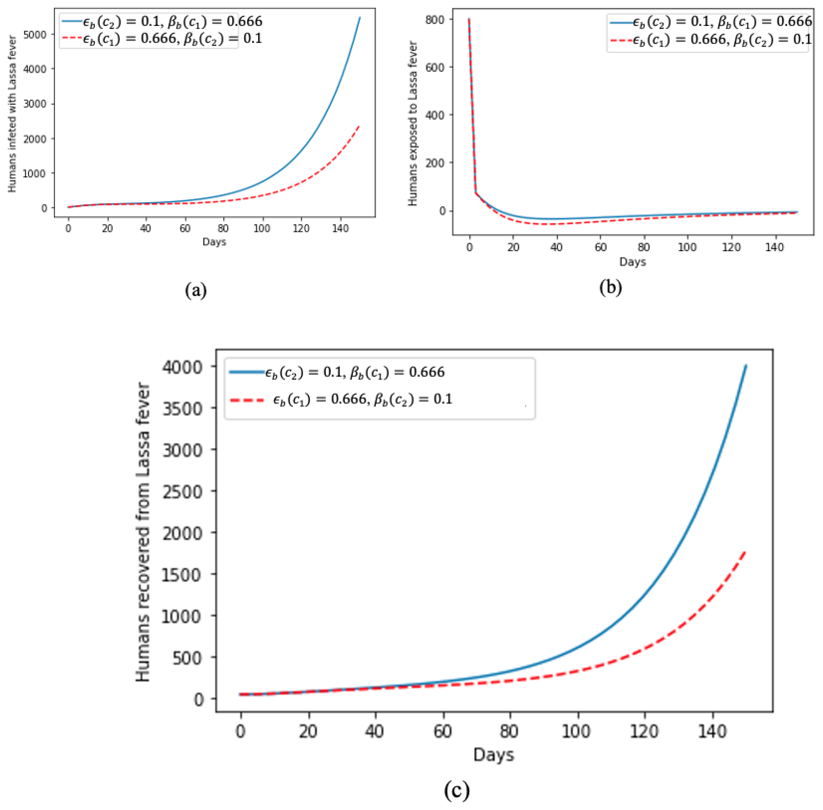
In Figure 3, we deduce how treatments help and accelerate recovery from Lassa fever, as can be seen in Figure 3c, as, despite the sharp increase in humans infected with the disease, as shown in Figure 3a, Figure 3b shows that, at the beginning of the disease spread, there was a spike in the number of humans exposed to Lassa fever disease but gradually tending towards zero as they are become diagnosed and isolated for treatment.
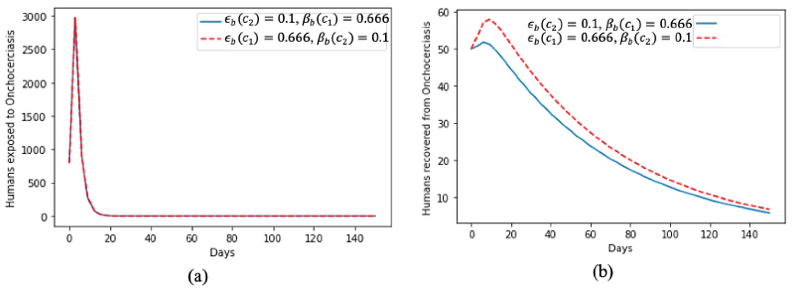
In Figure 4, we present the dynamics of the human exposure to onchocerciasis virus in Figure 4a; at the beginning of the time period, there was a huge spike; however, this later faded away and, despite the increase in the value of the rate of treatment and the proportion of effective treatment, the dynamics of the two curves remained the same throughout the time period. Figure 4b aligns with the results of human exposure to the disease, i.e., despite the spike at the beginning, a significant proportion of the human population recovered quickly but also showed that, if not properly treated and mitigated, it will take some time for people to recover from the onchocerciasis virus.
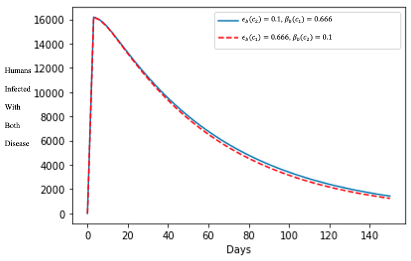
In Figure 5, after about 10 days, the number of humans infected with both diseases declined rapidly, showing the effects of treating the human population that are symptomatic to both diseases, and enabling the quick curtailment of its spread in the population even though varying the treatment rate parameters is insignificant in the shape of the epidemics.

6. Conclusions

In the previous work [19], the co-infection of malaria and Lassa fever was extensively analyzed on the optimal control; however, this work presents a co-infection model for OLF with periodic variational vectors and the model was extended to the optimal control model to analyze the impact of controls, especially in the treatment of infectious humans. This also represents an improvement on some of the studies in [26,27,28,29,30]. The model is qualitatively analyzed using both the model without control and model with control. We investigated the asymptotic behavior of the model without control and with respect to the equilibria. It is shown, using a Lyapunov function, that the disease-free equilibrium is globally asymptotically stable when the associated basic reproduction number is less than one. When it is greater than one, we prove the existence of a globally asymptotically stable endemic equilibrium with the aid of a suitable nonlinear Lyapunov function. Furthermore, using Pontryagin’s maximum principle, the necessary conditions for the existence of optimal control and the optimality system for the co-infection model are established. We showed that the optimal conditions and controls must be satisfied, and also proved that, from the invasion and coexistence of both diseases in their endemic states, it can be deduced that the protection against rodent, human interaction, and black fly biting rates reduces the reproduction number. The model without control is quantitatively analyzed by studying how sensitive the basic reproduction number is to the model parameters and the model simulation using the Runge–Kutta technique of order 4, which is also presented to study the effect of treatments. We deduced from the quantitative analysis that, if there is an effective treatment and diagnosis of those exposed and infected with the disease, the spread of the viral disease can be effectively managed, which is in agreement with the qualitative analysis of the control model. The limitation of this work is that obtaining real data for the co-infection of OLF disease did not allow us to fit our model to data to validate the model we developed, which will lead to one of our future works, i.e., fitting the model to data using one of the classical parameter-fitting methods like the particle filtering method. Another future work is to simulate the control model and extend the optimal control model by showing the effectiveness of control measures using the cost-effectiveness method. From the numerical graphs (Figure 3, Figure 4 and Figure 5), we can deduce that a reduction in the infected population, which infers that more treatment leads to a greater recovery in the population. From Figure 3, Figure 4 and Figure 5, it can be seen that the population having recovered from Lassa fever increases based on the impact of the treatment provided, while onchocerciasis recovery is slow, which implies that effective treatment is necessary due to the decline in the population dynamics. This also implies that the exposed or infected populations must be continuously treated so that there will not be a decline in the recovered population. However, the simulation results presented in this research gives some insight into the dynamics of the co-infection of onchocerciasis and Lassa fever virus, which can help guide public health officials in decision making, especially in sub-Saharan Africa where it is endemic. The numerical analysis varied the effect of treatment on the population dynamics of both diseases.

Author Contributions

Conceptualization, K.M.A.; methodology, K.O., U.M.A., K.M.A. and A.A.; software, K.O. and U.M.A.; validation, K.O.; formal analysis, K.O. and K.M.A.; investigation, K.O., K.M.A. and A.A.; resources, K.O. and A.A.; data curation, K.O., A.A. and U.M.A.; writing and original draft preparation, K.O. and K.M.A.; writing—review and editing, A.A. and K.O.; visualization, K.O., A.A. and U.M.A.; supervision, K.O.; project administration, K.O. All authors have read and agreed to the published version of the manuscript.

Funding

This research received no external funding.

Institutional Review Board Statement

Not applicable.

Informed Consent Statement

Not applicable.

Data Availability Statement

The code used for the simulation of the model used for this research is available upon request.

Acknowledgments

We appreciate our reviewers for their fruitful suggestions during the peer reviewing of this work.

Conflicts of Interest

The authors declare no conflicts of interest.

References

  1. Amazigo, U.; Noma, M.; Bump, J.; Bentin, B.; Liese, B.; Yameogo, L.; Zouré, H.; Seketeli, A. Chapter 15. In Onchocerciasis Disease and Mortality in Sub Saharan Africa; World Bank: Washington, DC, USA, 2006. [Google Scholar]
  2. Oguoma, I.C.; Acho, T.M. Mathematical modelling of the spread and control of onchocerciasis in tropical countries: Case study in Nigeria. Hindawi 2014, 2014, 631658. [Google Scholar] [CrossRef]
  3. Hassan, A.; Shaban, N. Onchocerciasis dynamics: Modelling the effects of treatment, education and vector control. J. Biol. Dyn. 2020, 14, 245–268. [Google Scholar] [CrossRef] [PubMed]
  4. World Health Organization. African programme for onchocerciasis control: Meeting of national onchocerciasis task forces, September 2012. Wkly. Epidemiol. Rec. 2012, 87, 494–502. [Google Scholar]
  5. Abioye, A.I.; Peter, O.J.; Ogunseye, H.A.; Oguntolu, F.A.; Oshinubi, K.; Ibrahim, A.A.; Khan, I. Mathematical model of COVID-19 in Nigeria with optimal control. Results Phys. 2021, 28, 104598. [Google Scholar] [CrossRef] [PubMed]
  6. Oshinubi, K.; Peter, O.J.; Addai, E.; Mwizerwa, E.; Babasola, O.; Nwabufo, I.V.; Sane, I.; Adam, U.M.; Adeniji, A.; Agbaje, J.O. Mathematical Modelling of Tuberculosis Outbreak in an East African Country Incorporating Vaccination and Treatment. Computation 2023, 11, 143. [Google Scholar] [CrossRef]
  7. Mopecha, J.P.; Thieme, H.R. Competitive Dynamics in a Model for Onchocerciasis with Cross-Immunity. Can. Appl. Math. Q. 2003, 11, 339–376. [Google Scholar]
  8. Peter, O.J.; Ibrahim, M.O.; Edogbanya, H.O.; Oguntolu, F.A.; Oshinubi, K.; Ibrahim, A.A.; Ayoola, T.A.; Lawal, J.O. Direct and indirect transmission of typhoid fever model with optimal control. Results Phys. 2021, 27, 104463. [Google Scholar] [CrossRef]
  9. Basáñez, M.-G.; Ricárdez-Esquinca, J. Models for the population biology and control of human onchocerciasis. Trends Parasitol. 2001, 17, 430–438. [Google Scholar] [CrossRef]
  10. Ngungu, M.; Addai, E.; Adeniji, A.; Adam, U.M.; Oshinubi, K. Mathematical epidemiological modeling and analysis of monkeypox dynamism with non-pharmaceutical intervention using real data from United Kingdom. Front. Public Health 2023, 11, 1101436. [Google Scholar] [CrossRef]
  11. Niger, A.M.; Gumel, A.B. Mathematical analysis of the role of repeated exposure on malaria transmission dynamics. Differ. Equ. Dyn. Syst. 2008, 16, 251–287. [Google Scholar] [CrossRef]
  12. Pontryagin, L.S.; Boltyanskii, V.T.; Gamkrelidze, R.V.; Mischeuko, E.F. The mathematical Theory of Optimal Processes; Selected Works IV; Gordon and Breach Science Publishers: New York, NY, USA, 1986. [Google Scholar]
  13. Plaisier, A.P.; Alley, E.S.; van Oortmarssen, G.J.; Boatin, B.A.; Habbema, J.D.F. Required duration of combined annual ivermectin treatment and vector control program in west Africa. Bull. World Health Organ. 1997, 75, 237. [Google Scholar] [PubMed]
  14. Remme, J.; Sole, G.D.; van Oortmarssen, G.J. The predicted and observed decline in onchocerciasis infection during 14 years of successful control of black flies in West Africa. Bull. World Health Organ. 1990, 68, 331–339. [Google Scholar]
  15. Bawa, M.; Abdulrahman, S.; Jimoh, O.R.; Adabara, N.U. Stability analysis of disease free equilibrium state for Lassa fever disease. J. Sci. Technol. Math. Educ. 2012, 9, 115–123. [Google Scholar]
  16. Tomori, O.; Fabiyi, A.; Sorungbe, A.; Smith, A.; Cormick, J.B. Viral hemorrhagic fever antibodies in Nigeria populations. Am. J. Trop. Med. Hyg. 1998, 38, 407–410. [Google Scholar] [CrossRef]
  17. den Driessche, P.V.; Watmough, J. Reproduction numbers and subthreshold endemic equilibria for compartmental models of disease transmission. Math. Biosci. 2002, 180, 29–48. [Google Scholar] [CrossRef] [PubMed]
  18. James, T.O.; Abdulrahman, S.; Akinyemi, S.; Akinwande, N.I. Dynamics transmission of Lassa fever. Int. J. Innov. Res. Educ. Sci. 2015, 2, 2349–5219. [Google Scholar]
  19. Onifade, A.A. Subharmonic Bifurcation in Malaria-Lassa Fever Co-Infection Epidemic Model with Optimal Control Application. Ph.D. Thesis, University of Ibadan, Ibadan, Nigeria, 2021. [Google Scholar]
  20. McKendrick, J.Q.; Tennant, W.S.; Tildesley, M.J. Modelling seasonality of Lassa fever incidences and vector dynamics in Nigeria. PLoS Neglected Trop. Dis. 2023, 17, e0011543. [Google Scholar] [CrossRef]
  21. Cheke, R.A.; Sowah, S.A.; Avissey, H.S.; Fiasorgbor, G.K.; Garms, R. Seasonal variation in onchocerciasis transmission by Simulium squamosum at perennial breeding sites in Togo. Trans. R. Soc. Trop. Med. Hyg. 1992, 86, 67–71. [Google Scholar] [CrossRef]
  22. Blayneh, K.W.; Cao, Y.; Kwon, H.-D. Optimal control of vector-borne diseases: Treatment and prevention. Discret. Contin. Dyn. Syst. B 2009, 11, 587–611. [Google Scholar] [CrossRef]
  23. Okuonghae, D.; Okuonghae, R.A. Mathematical model for Lassa fever. J. Niger. Assoc. Math. Phys. 2006, 10, 457–464. [Google Scholar] [CrossRef]
  24. Ogabi, C.O.; Olusa, T.V.; Madufor, M.O. Controlling Lassa Fever Transmission in Northern Part of Edo State, Nigeria Using Sir Model. N. Y. Sci. J. 2012, 5, 190–197. [Google Scholar]
  25. Adeniji, A.A.; Noufe, H.A.; Mkolesia, A.C.; Shatalov, M.Y. An Approximate Solution to Predator-prey Models Using The Differential Transform Method and Multi-step Differential Transform Method, in Comparison with Results of The Classical Runge-kutta Method. Math. Stat. 2021, 9, 799–805. [Google Scholar]
  26. Smith, M.E.; Bilal, S.; Lakwo, T.L.; Habomugisha, P.; Tukahebwa, E.; Byamukama, E.; Katabarwa, M.N.; Richards, F.O.; Cupp, E.W.; Unnasch, T.R.; et al. Accelerating river blindness elimination by supplementing MDA with a vegetation “slash and clear” vector control strategy: A data-driven modeling analysis. Sci. Rep. 2019, 9, 15274. [Google Scholar] [CrossRef] [PubMed]
  27. Alley, W.S.; van Oortmarssen, G.J.; Boatin, B.A.; Nagelkerke, N.J.; Plaisier, A.P.; Remme, J.H.; Lazdins, J.; Borsboom, G.J.; Habbema, J.D.F. Macrofilaricides and onchocerciasis control, mathematical modelling of the prospects for elimination. BMC Public Health 2001, 1, 12. [Google Scholar] [CrossRef] [PubMed]
  28. Hamley, J.I.D.; Milton, P.; Walker, M.; Basáñez, M.G. Modelling exposure heterogeneity and density dependence in onchocerciasis using a novel individual-based transmission model, EPIONCHO-IBM: Implications for elimination and data needs. PLoS Neglected Trop. Dis. 2019, 13, e0007557. [Google Scholar] [CrossRef]
  29. Bako, D.U.; Akinwande, N.I.; Enagi, A.I.; Kuta, F.A.; Abdulrahman, S. Stability Analysis of a Mathematical Model for Onchocerciaisis Disease Dynamics. J. Appl. Sci. Environ. Manag. 2017, 21, 663–671. [Google Scholar] [CrossRef]
  30. Hamley, J.I.D.; Walker, M.; Coffeng, L.E.; Milton, P.; de Vlas, S.J.; Stolk, W.A.; Basáñez, M. Structural Uncertainty in Onchocerciasis Transmission Models Influences the Estimation of Elimination Thresholds and Selection of Age Groups for Seromonitoring. J. Infect. Dis. 2020, 221 (Suppl. S5), S510–S518. [Google Scholar] [CrossRef]
Figure 1. Graph of parameters and their sensitivity indices.
Appliedmath 04 00006 g001
Figure 2. Graph of parameters and their sensitivity indices.
Appliedmath 04 00006 g002
Figure 3. Effect of treatment on (a) humans infected by Lassa fever; (b) humans exposed to Lassa fever; and (c) humans that recovered from Lassa fever.
Appliedmath 04 00006 g003
Figure 4. Effect of treatment on (a) humans exposed to onchocerciasis and (b) humans that recovered from onchocerciasis.
Appliedmath 04 00006 g004
Figure 5. Effect of the treatment of humans infected with both diseases.
Appliedmath 04 00006 g005
Table 1. The definitions of the parameters in model (1).
DefinitionSymbols
Susceptible to human recruitment ζ ( c i )
Susceptible to black fly recruitment ς b
Susceptible term for rodent recruitment Λ r ( d j )
Rate of black fly bitingb
Rodent interaction rate w 2 ( d j )
Human interaction rate w 1 ( c i )
Onchocerciasis transmission rate in humans c b ( c i )
Onchocerciasis transmission rate in black flies σ b
Lassa fever transmission rate in individuals by infectious individuals d 1 ( c i )
Lassa fever transmission rate in individuals by infectious rodents d 2 ( c i )
Lassa fever transmission rate in rodents by infected rodents β r ( d j )
Human mortality rate per capita μ ( c i )
Black fly mortality rate per capita μ b
Rodent death rate per capita μ r ( d j )
Rodent mortality rate due to hunting δ r ( d j )
Black fly seasonal variation κ b
Rodent seasonal fluctuation ξ r
Lassa fever progression rate in an exposed individual τ ( c i )
Onchocerciasis progression rate in the exposed human host τ b ( c i )
Lassa fever progression rate in exposed rodents α r ( d j )
Onchocerciasis progression rate in exposed black flies α b
The proportion of effective human onchocerciasis treatment ϵ b ( c i )
Infectious human onchocerciasis treatment rate β b ( c i )
Proportion of successful Lassa fever treatment for exposed humans γ v ( c i )
Lassa fever diagnostic tests for humans who have been exposed α ( c i )
Proportion of successful Lassa fever treatment for infected humans σ ( c i )
Infectious human Lassa fever treatment rate η v ( c i )
Force of infection for Lassa fever in humans by infectious humans λ a
Force of infection for Lassa fever in humans by infectious rodents λ b
Force of infection for Lassa fever in rodent population by infectious rodents λ r
Onchocerciasis infection rate λ B
Rate of recovery from Lassa fever ϑ r
Rate of recovery from onchocerciasis ϑ b
Rate of loss of immunity to onchocerciasis γ b ( c i )
Table 2. The parameter values of the OLF co-infection model.
SymbolsValueSource
ζ ( c i ) 0.000212Estimated
ς b 0.065[11]
Λ r ( d j ) 0.0054[16]
b0.8Fixed
w 2 ( d j ) 0.75Assumed
w 1 ( c i ) 0.55Assumed
c b ( c i ) 0.099[22]
σ b 0.089[22]
d 1 ( c i ) 0.00814[22]
d 2 ( c i ) 0.055[16]
β r ( d j ) 0.073Assumed
μ ( c i ) 0.0000545Estimated
μ b 0.0665Estimated
μ r ( d j ) 0.058[23]
δ r ( d j ) 0.295Assumed
κ b 0.5Assumed
ξ r 0.00021Assumed
τ ( c i ) 0.082[24]
τ b ( c i ) 0.0585Assumed
α r ( d j ) 0.83Assumed
α b 0.0554Assumed
ϵ b ( c i ) 0–0.1Assumed to vary
β b ( c i ) 0–0.1Assumed to vary
γ v ( c i ) 0.09Assumed
α ( c i ) 0.049Assumed
σ ( c i ) 0–0.189Assumed to vary
η v ( c i ) 0.43Assumed
γ b ( c i ) 0.0013692Assumed
ϑ r 0–0.2Assumed to vary
ϑ b 0–0.3Assumed to vary
λ a 0–0.2Assumed to vary
λ b 0–0.3Assumed to vary
λ r 0–0.5Assumed to vary
λ B 0–0.4Assumed to vary
Table 3. Parameter sensitivity index for R 0 L ( t , c ) .
ParametersSensitivity Index
σ ( c i ) 1
ω ( c i ) 0.828483245781356
ζ ( c i ) 1
τ ( c i ) 0.849041859804287
η ( c i ) 0.967222373292614
μ ( c i ) 1.06060720384700
σ ( c i ) 0.967222373292614
γ v ( c i ) 0.821212282664678
α ( c i ) 0.821212282664678
Table 4. Parameter Sensitivity Index of R 0 B ( t , a ) .
ParametersSensitivity Index
α b 0.498408501754949
ς b 0.5
ρ ( c i ) 0.5
τ b ( c i ) 0.105493469772452
ζ ( c i ) 0.5
b 1.02094596559
κ ( c i ) 0.361379512214456
μ b 1.42094596559
μ ( c i ) 1.12094596559
β b ( c i ) 0.12094596559
Disclaimer/Publisher’s Note: The statements, opinions and data contained in all publications are solely those of the individual author(s) and contributor(s) and not of MDPI and/or the editor(s). MDPI and/or the editor(s) disclaim responsibility for any injury to people or property resulting from any ideas, methods, instructions or products referred to in the content.

