A Mathematical Structure Underlying Sentences and Its Connection with Short–Term Memory

Matricciani, Emilio

doi:10.3390/appliedmath4010007

Open AccessArticle

A Mathematical Structure Underlying Sentences and Its Connection with Short–Term Memory

by

Emilio Matricciani

Dipartimento di Elettronica, Informazione e Bioingegneria (DEIB), Politecnico di Milano, 20133 Milan, Italy

AppliedMath 2024, 4(1), 120-142; https://0-doi-org.brum.beds.ac.uk/10.3390/appliedmath4010007

Submission received: 9 December 2023 / Revised: 12 January 2024 / Accepted: 15 January 2024 / Published: 18 January 2024

Download

Browse Figures

Versions Notes

Abstract

:

The purpose of the present paper is to further investigate the mathematical structure of sentences—proposed in a recent paper—and its connections with human short–term memory. This structure is defined by two independent variables which apparently engage two short–term memory buffers in a series. The first buffer is modelled according to the number of words between two consecutive interpunctions—variable referred to as the word interval,

I_{P}

—which follows Miller’s

7 \pm 2

law; the second buffer is modelled by the number of word intervals contained in a sentence,

M_{F}

, ranging approximately for one to seven. These values result from studying a large number of literary texts belonging to ancient and modern alphabetical languages. After studying the numerical patterns (combinations of

I_{P}

and

M_{F}

) that determine the number of sentences that theoretically can be recorded in the two memory buffers—which increases with the use of

I_{P}

and

M_{F}

—we compare the theoretical results with those that are actually found in novels from Italian and English literature. We have found that most writers, in both languages, write for readers with small memory buffers and, consequently, are forced to reuse sentence patterns to convey multiple meanings.

Keywords:

alphabetical languages; extended short–term memory; human communication; human mind; sentences; mathematical modeling; universal readability index

1. Does the Short–Term Memory Process Words with Two Independent Buffers in Series?

Recently [1], we proposed a well–grounded conjecture that a sentence—read or pronounced as the two activities are similarly processed by the brain [2]—is elaborated by the short–term memory (STM), with two independent processing units in series that have similar buffer size. The clues for conjecturing this model have emerged from considering many novels belonging to Italian and English literature. In [1], we have shown that there are no significant mathematical/statistical differences between the two literary corpora, according to surface deep–language variables. In other words, the mathematical surface structure of alphabetical languages—a creation of the human mind—seems to be deeply rooted in humans, independent of the particular language used.

A two–unit STM processing can be justified according to how a human mind seems to memorize “chunks” of information written in a sentence. Although simple and related to the surface of language, the model seems to describe mathematically the input–output characteristics of a complex mental process largely unknown.

According to [1], the first processing unit is linked to the number of words between two contiguous interpunctions, the variable for which is indicated by

I_{p}

—termed the word interval (Appendix A lists the mathematical symbols used in the present paper)—approximately ranging within Miller’s

7 \pm 2

law range [3,4,5,6,7,8,9,10,11,12]. The second unit is linked to the number

M_{F}

of

I_{p}

s contained in a sentence, referred to as the extended STM, or E–STM, ranging approximately from one to six. We have shown that the capacity (expressed in words) required to process a sentence ranges from

8.3

to

61.2

words, values that can be converted into time by assuming a reading speed. This conversion gives the range

2.6 ~ 19.5

s for a fast reader [13], and

5.3 ~ 30.1

s for an average reader of novels, values that are well-supported by the experiments reported in the literature [14,15,16,17,18,19,20,21,22,23,24,25,26,27,28,29].

The E–STM must not be confused with the intermediate memory [30,31]. It is not modelled by studying neuronal activity, but by studying the surface aspects of human communication, such as words and interpunctions, whose effects writers and readers have experienced since the invention of writing.

The modeling of the STM processing by two units in a series has never been considered in the literature before [1,32]. The reader is very likely aware that the literature on the STM and its various aspects is very large and multidisciplinary, but nobody—as far as we know—has never considered the connections we have found and discussed in [1,32]. Moreover, a sentence conveys meaning; therefore, the theory we are further developing in the present paper might be a starting point to arrive at the information theory that includes meaning.

Currently, some attempts are being made by many scholars to arrive at a “semantic communication” theory or a “semantic information” theory, but the results are still, in our opinion, in their infancies [33,34,35,36,37,38,39,40,41]. These theories, as those concerning the STM, have not considered the main “ingredients” of our theory—namely

I_{P}

and

P_{F}

—as a starting point for including meaning, which is still a very open issue.

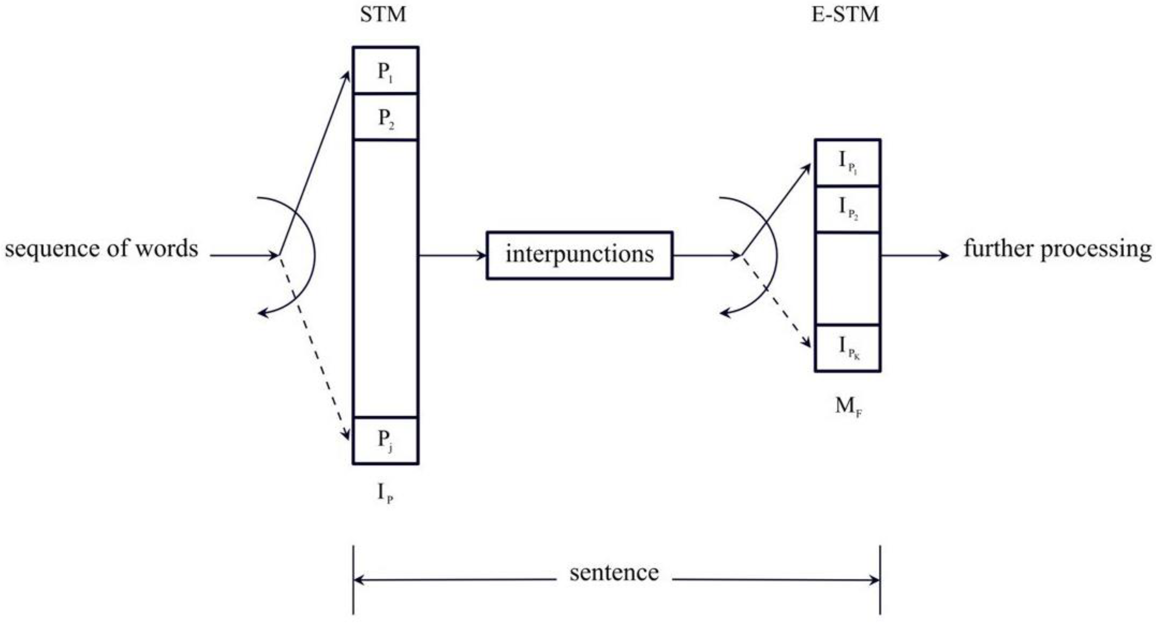
Figure 1 sketches the flowchart of the two processing units [1]. The words

p_{1}

,

p_{2}

,…

p_{j}

are stored in the first buffer up to

j

items—approximately in Miller’s range—until an interpunction is introduced to fix the length of

I_{P}

. The word interval

I_{P}

is then stored in the second buffer up to

k

items, from about one to six, until the sentence ends. The process is then repeated for the next sentence.

The purpose of the present paper is to further investigate the mathematical structure underlying sentences, both theoretically and experimentally, by considering the novels previously mentioned [1] listed in Table A1 for Italian literature and in Table A2 for English literature.

After this introduction, in Section 2, we study the probability distribution function (PDF) of sentence size—measured in words—that is recordable by an E–STM buffer made of

C_{F}

cells (this parameter plays the role of

M_{F}

). In other words, in this section, we study and discuss the length of sentences that humans can possibly conceive with an E–STM made of

C_{F}

memory cells.

In Section 3, we study the number of sentences, with the same number of words, that

C_{F}

cells can process. In this section, we study and discuss the complementary issue of Section 2, namely, how many sentences with a constant number of words humans can conceive, based solely on the E–STM of

C_{F}

cells.

In Section 4, we compare the number of sentences that authors of Italian and English literature actually wrote for their novels to the number of sentences theoretically available to them, by defining a multiplicity factor. In Section 5, we define a mismatch index, which synthetically measures to what extent a writer uses the number of sentences that are theoretically available. In Section 6, we show that the parameters studied increase with the year of novel publication. Finally, in Section 7, we summarize the main results and propose future work.

2. Probability Distribution of Sentence Length versus E–STM Buffer Size

First, we study the conditional PDF of sentence length, measured in words

W

—i.e., the parameter which in long texts, such as chapters, gives

P_{F}

of each chapter—recordable in an E–STM buffer made of

C_{F}

cells, i.e., the parameter which gives

M_{F}

in chapters. Second, we study the overlap of the PDFs because this overlap gives interesting indications.

2.1. Probability Distribution of Sentence Length

To estimate the PDF of sentence length, we run a Monte Carlo simulation based on the PDF of

I_{P}

obtained in [1] by merging the two literatures listed in Section 1.

In [1], we have shown that the PDF of

I_{P}

,

P_{F}

and

M_{F}

—as previously mentioned, these averages refer to single chapters of the novels—can be modelled with a three-parameter log–normal density function [42] (natural logs):

f (x) = \frac{1}{\sqrt{2 π} σ_{x} (x - 1)} \exp \{- \frac{1}{2} {[\frac{\ln (x - 1) - μ_{x})}{σ_{x}}]}^{2}\} x \geq 1

(1)

In Equation (1),

μ_{x}

and

σ_{x}

are, respectively, the mean value and the standard deviation the log–normal PDF. Table 1 reports these values for the three deep-language variables.

The Monte Carlo simulation steps are as follows:

Consider a buffer made of $C_{F}$ cells. The sentence contains $C_{F}$ word intervals: for example, if $C_{F} = 3$ , the sentence contains two interpunctions followed by a full stop, a question mark, or an exclamation mark.
Generate $C_{F}$ independent values of $I_{P}$ according to the log–normal model given by Equation (1) and Table 1. The independence of $I_{P}$ from a cell to another cell is reasonable [1]. In detail, from a random number generator of standard Gaussian density variables $X_{i}$ (zero mean and unit standard deviation), we get the relationship $X_{i} = (y_{i} - μ_{x}) / σ_{x}$ ; therefore, the three-parameter log–normal variable $I_{P, i} \geq 1$ is then given by $I_{P, i} = \exp (y_{i}) + 1 = \exp (σ_{x} X_{i} + μ_{x}) + 1$ .
Add the number of words contained in the $C_{F}$ cells to obtain $W$ :

$W = \sum_{i = 1}^{C_{F}} I_{p, i}$

(2)
Repeat steps one through three many times (we repeated these steps 100,000 times, i.e., we simulated 100,000 sentences of different length) to obtain a stable conditional PDF of $W$ .
Repeat steps one through four for another $C_{F}$ and obtain another PDF.

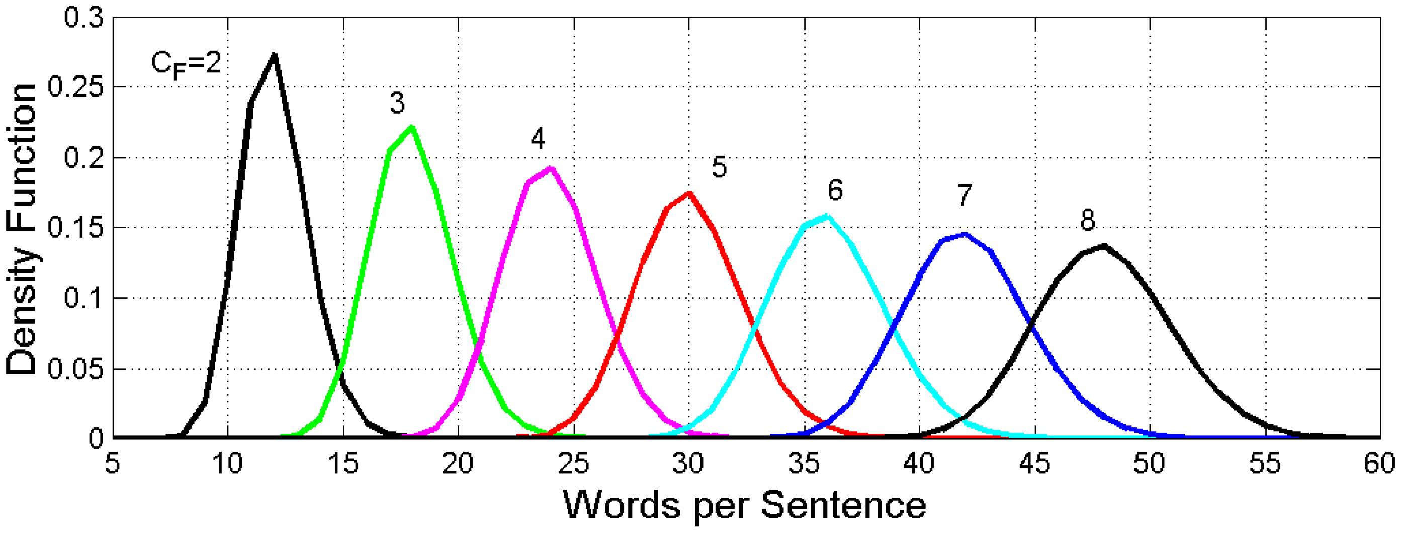
Figure 2 shows the conditional PDF for several values of

C_{F}

. Each PDF can be very well-modelled by a Gaussian PDF

f_{C_{F}} (x)

because the probability of getting unacceptable negative values is negligible in any of the PDFs shown in Figure 2. For example, for

C_{F} = 3

, the mean value and the standard deviation are, respectively,

m_{3} = 18.00

words and

s_{3} = 1.79

words.

In general terms [42], the mean value of Equation (2) is given by:

m_{C_{F}} = <W> = <\sum_{i = 1}^{C_{F}} I_{p, i}> = \sum_{i = 1}^{C_{F}} <I_{P, i}> = C_{F} <I_{p}>

(3)

Therefore,

m_{C_{F}}

is proportional to

C_{F}

. As for the standard deviation of

W

, if the

I_{p, i}

’s are independent—as we assume—then the variance

s_{C_{F}}^{2}

of

W

is given by:

s_{C_{F}}^{2} = \sum_{i = 1}^{C_{F}} σ_{I_{P, i}}^{2} = C_{F} \times σ_{I_{P}}^{2}

(4)

Therefore, the standard deviation

s_{C_{F}}

is proportional to

\sqrt{C_{F}}

. Finally, according to the central limit theory [42], the PDF can be modelled as Gaussian in a significant range about the mean.

In conclusion, the Monte Carlo simulation produces a Gaussian PDF with a mean value proportional to

C_{F}

and a standard deviation proportional to

\sqrt{C_{F}}

. These findings are clearly evident in the PDFs shown in Figure 2, in which

m_{C_{F}}

and

s_{C_{F}}

increase as theoretically expected; therefore, the mean values and standard deviations of the other PDFs can be calculated by scaling the values found for

C_{F} = 3

. For example, for

C_{F} = 6

,

m_{6} = 2 \times 18.00 = 36.00

words and

s_{6} = \sqrt{2} \times 1.79 = 2.53

words.

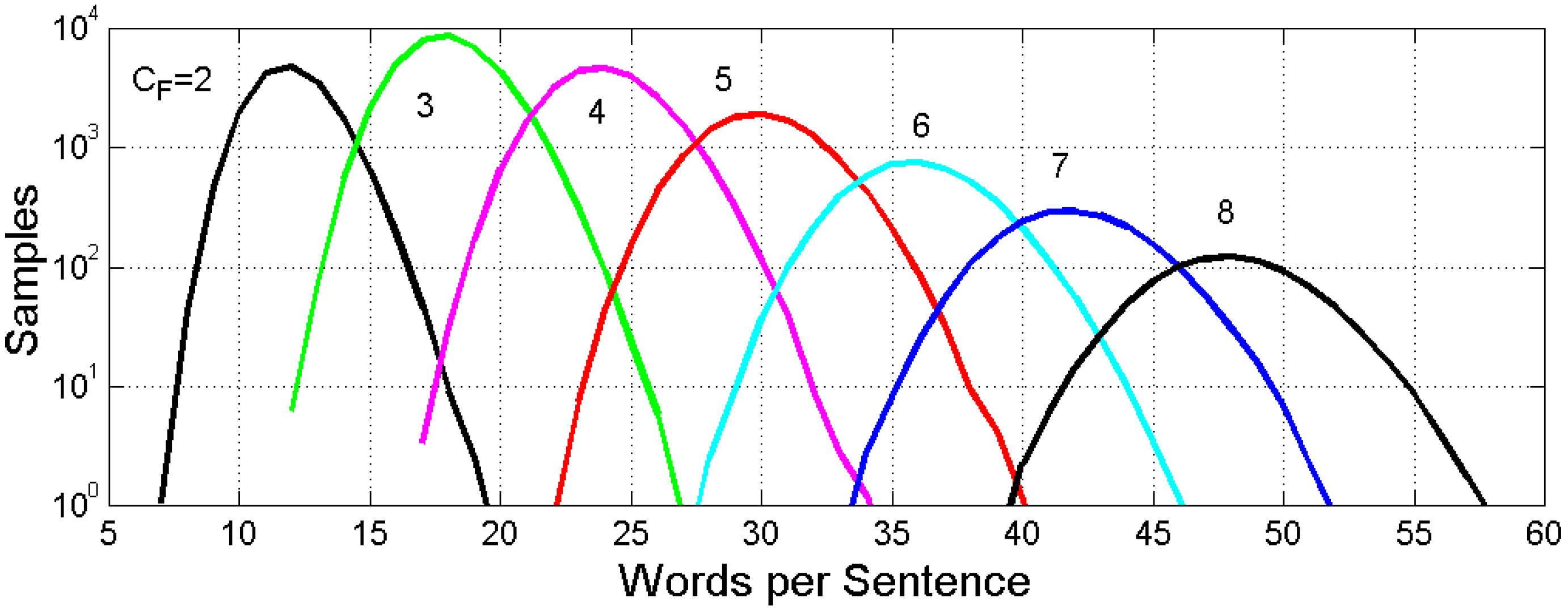
Figure 3 shows the histograms corresponding to Figure 2. The number of samples for each conditional PDF, out of 100,000 considered in the Monte Carlo simulation, is obtained by distributing the samples according to the PDF of

M_{F}

given by Equation (1) and Table 1. The case

C_{F} = 3

gives the largest sample size.

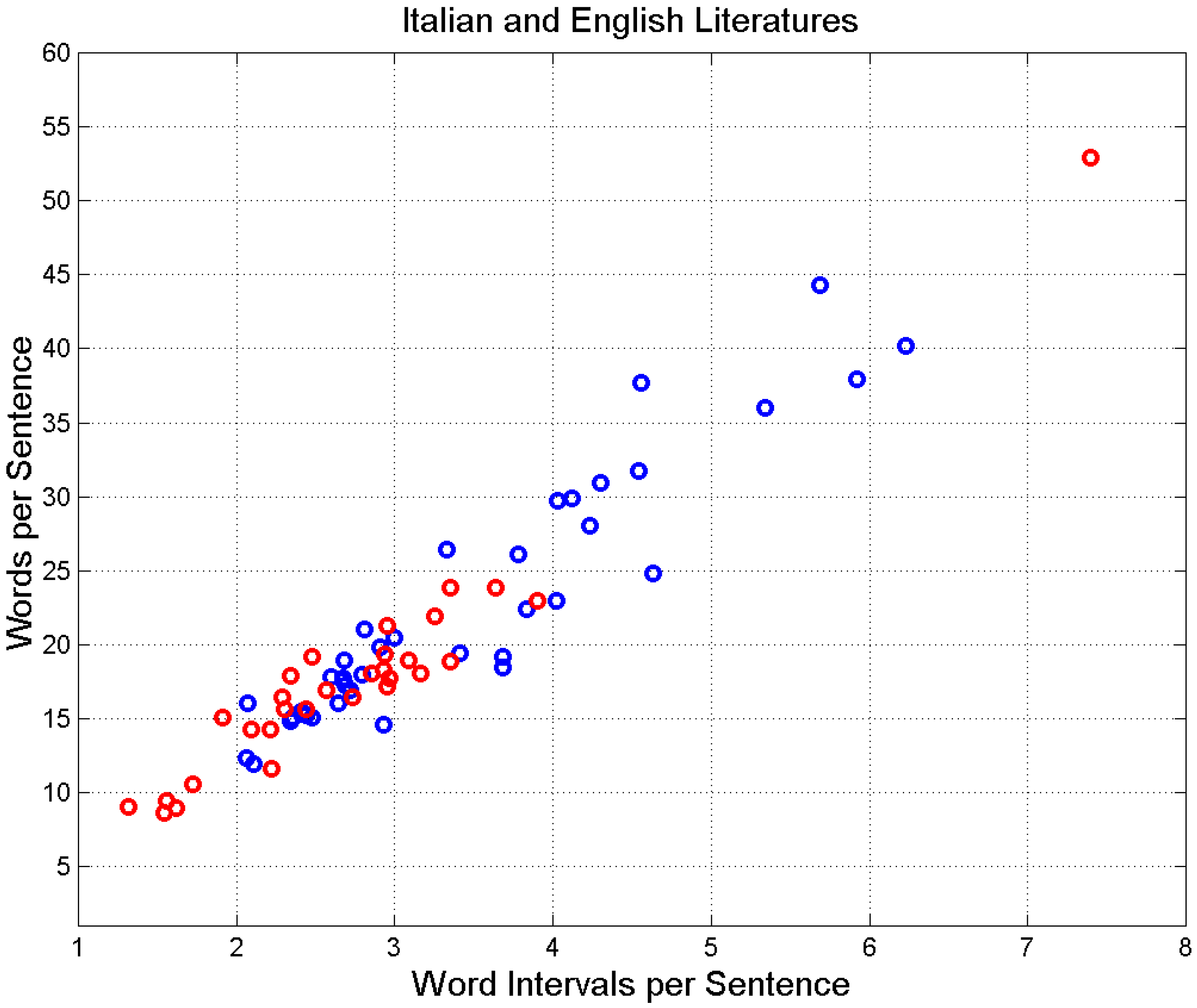
The results shown above have an experimental basis because the relationship between

<P_{F}>

, the average of words per sentence for the entire novel which is calculated by averaging the

P_{F}

of single chapters via weighting single chapters with the fraction of novel total word, as discussed in [32], versus

< M_{F} >

, the average of

M_{F}

of a novel calculated as

P_{F},

is linear, as Figure 4 shows by drawing

<P_{F}>

versus

<M_{F}>

concerning the Italian and English novels mentioned above.

2.2. Overlap of the Conditional Probability Distributions

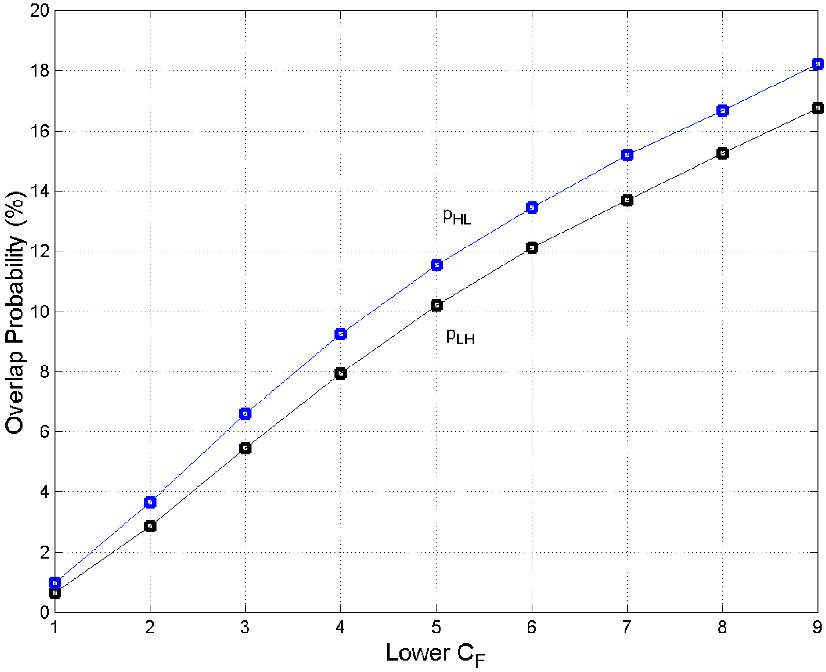
Figure 2 shows that the conditional PDFs overlap; therefore, some sentences can be processed by buffers of diverse

C_{F}

size, either larger or smaller. Let us define the probability of these overlaps.

Let

W_{t h}

be the intersection of two contiguous Gaussian PDFs, for example,

f_{C_{F} - 1} (x)

and

f_{C_{F}} (x)

; therefore, the probability

p_{H L}

that a sentence length can be found in the nearest lower Gaussian PDF (going from

C_{F} \to C_{F} - 1

) is given by [42]:

p_{H L} = \int_{- \infty}^{W_{t h}} f_{C_{F}} (x) d x \approx \int_{0}^{W_{t h}} f_{C_{F}} (x) d x

(5)

Similarly, the probability that a sentence length can be found in the nearest higher Gaussian PDF (going from

C_{F} - 1 \to C_{F}

) is given by:

p_{L H} = \int_{W_{t h}}^{\infty} f_{C_{F} - 1} (x) d x

(6)

For example, the threshold value between

f_{C_{F = 3}} (x)

and

f_{C_{F = 4}} (x)

is

W_{t h} = 20.9

words and

p_{H L} = 6.6 %

, while

p_{L H} = 5.5 %

.

Figure 5 draws these probabilities (%) versus

C_{F} - 1

(lower

C_{F}

). Because

s_{C_{F}}

increases with

\sqrt{C_{F}}

, therefore

p_{H L} > p_{L H}

. However, this is not only a mathematically obvious result, but it also meaningful because it indicates that: (a) a human mind can process sentences of lengths belonging to the contiguous lower or higher

M_{F}

(the probability of going to more distant PDFs is negligible) and (b) the number of these sentences is larger in the case

C_{F} \to C_{F} - 1

, which simply means that an E–STM buffer can process to a larger extent data matched to a smaller capacity buffer than data matched to a larger capacity buffer.

Finally, notice that each sentence conveys meaning—theoretically, any sequence of words might be meaningful, although this may not always be the case, but we do not know the proportion—therefore, the PDFs found above are also the PDFs associated with meaning. Moreover, the same numerical sequence of

W

words can carry different meanings, according to the words used. Multiplicity of meaning, therefore, is “built in” in a sequence of

W

words. We will further explore this issue in the next sections by considering the number of sentences that authors of Italian and English literature actually wrote.

So far, we have explored the processing of the words of a sentence by simulating sentences of diverse length that are conditioned to the E–STM buffer size. In the next section, we explore the complementary processing concerning the number of sentences that contain the same number of words.

3. Theoretical Number of Sentences Recordable in $C_{F}$ Cells

We study the number of sentences of

W

words that an E–STM buffer, made of

C_{F}

cells, can theoretically process. In summary, we ask the following question: how many sentences

S_{W}^{(C_{F})}

containing the same number of words

W

(Equation (2)) can be theoretically written in

C_{F}

cells?

Table 2 reports these numbers as a function of

W

and

C_{F}

. We calculated these data first by running a code and then by finding the mathematical recursive formula that generates them, given by the following:

S_{W}^{(C_{F})} = S_{W - 1}^{(C_{F})} + S_{W - 1}^{(C_{F} - 1)}

(7)

For example, if

W = 20

words and

C_{F} = 4

, we read

S_{19}^{(C_{F} = 4)} = 816

and

S_{19}^{(C_{F} - 1 = 3)} = 153

; therefore,

S_{20}^{(C_{F} = 4)} = 816 + 153 = 969

.

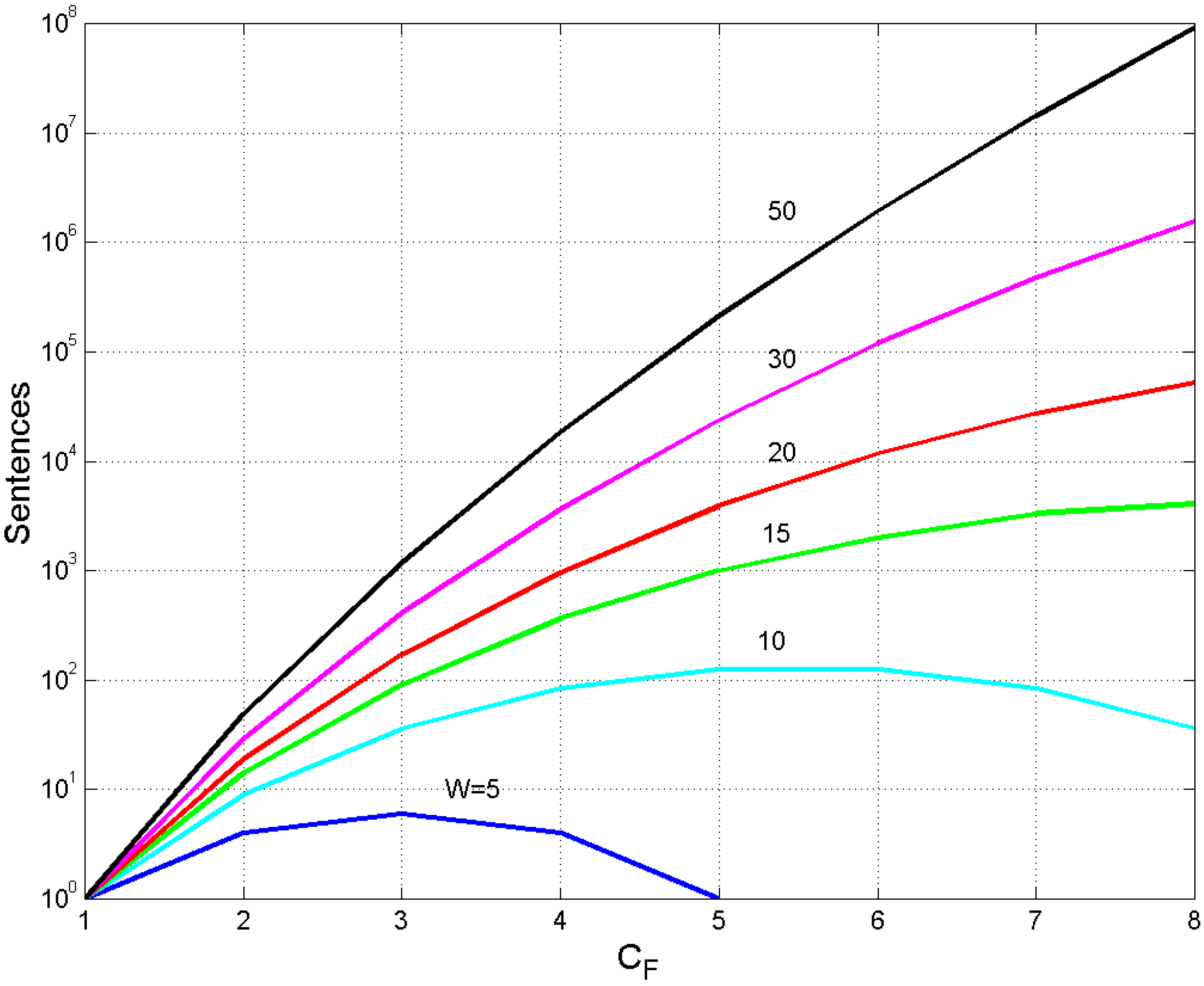
Figure 6 draws the data reported in some lines of Table 2 for a quick overview. We see how fast the number of sentences changes with

C_{F}

for constant

W

. For example, if

W = 20

words, then

S_{W = 20}

ranges from 1 (

C_{F} = 1)

to 52,698 sentences (

C_{F} = 8)

. Maxima are clearly visible for

W = 5

and

W = 10

words at

C_{F} = 3

and

C_{F} = 5 or 6

, respectively. Values become fantastically large for larger

W

and

C_{F}

, well beyond the ability and creativity of single writers, as we will show in Section 4.

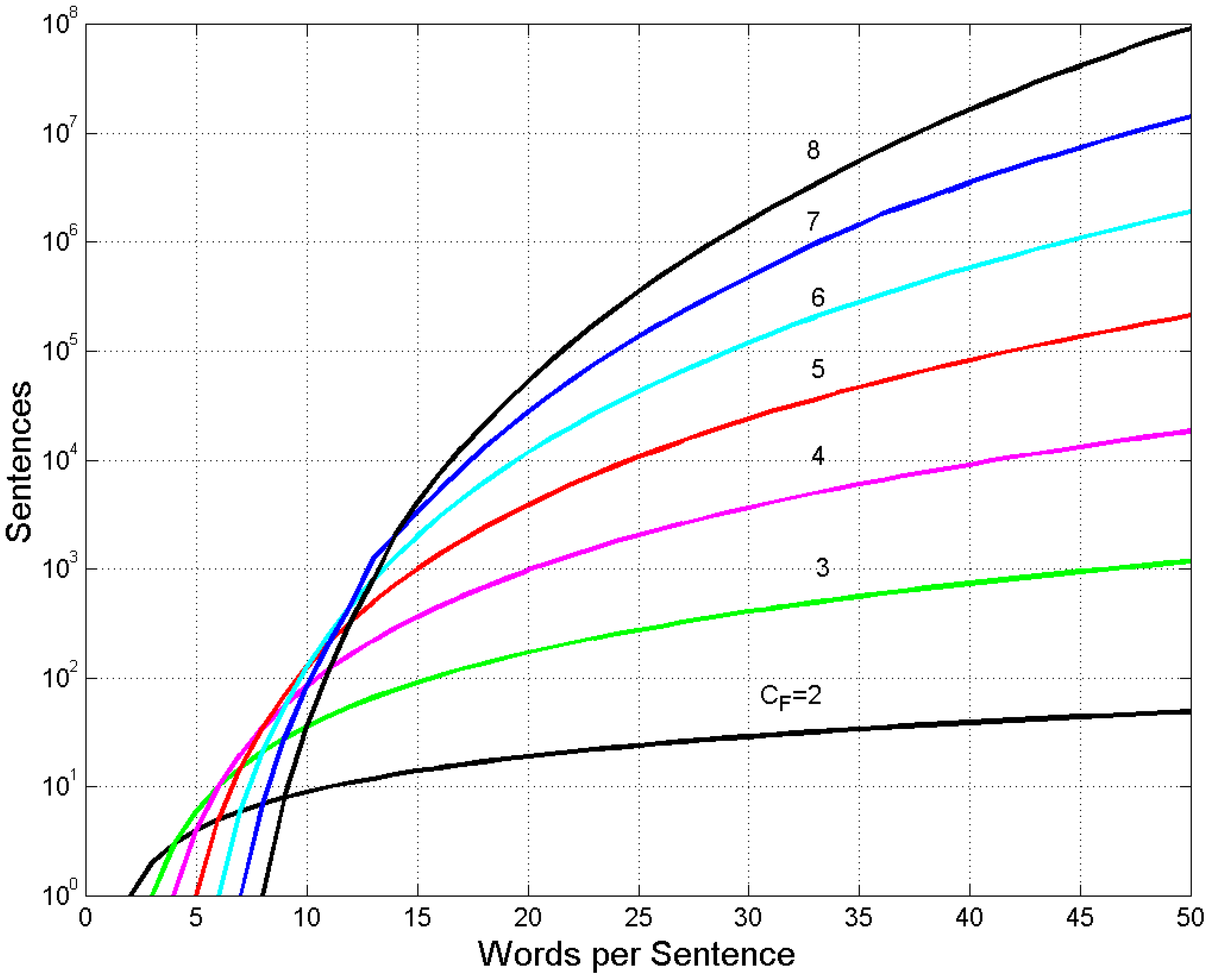
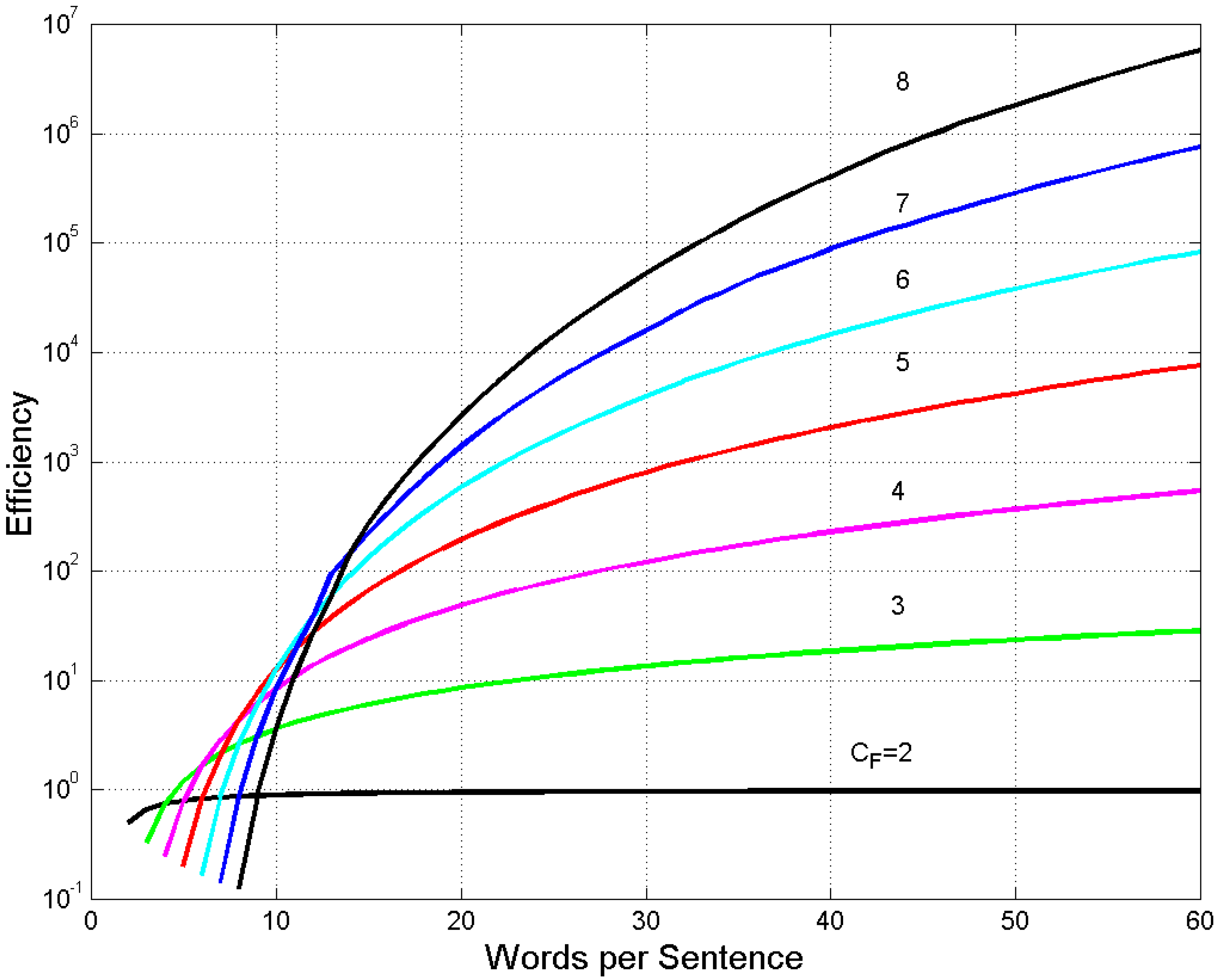
Figure 7 draws the data reported in some columns of Table 2, i.e., the number of sentences

S_{W}^{(C_{F})}

versus

W

, for fixed

C_{F}

. In this case, it is useful to adopt an efficiency factor

ε

, which is defined as the ratio between

S_{W}^{(C_{F})}

and

W

for a given

C_{F}

:

ε = \frac{S_{W}^{(C_{F})}}{W}

(8)

This factor explains, summarily, how a buffer of

C_{F}

cells is efficient in providing sentences with a given number of words, its units being sentences per word.

Figure 8 shows

ε

versus

W

. It is interesting to note that for

W ≲ 10

words, the buffer

C_{F} = 2

can be more efficient than the others. Beyond

W = 10

, the larger buffers become very efficient with very large

ε

.

If a writer uses short buffers—e.g., deliberately because of his/her style, or necessarily because of the reader’s E–STM memory size—then he/she has to repeat the same numerical sequence of words many times, according to the number of meanings conveyed. For example, if

C_{F} = 2

and

W = 10,

the writer has only nine different choices, or patterns, of two numbers whose sum is 10 (Table 2). Therefore, Table 2 gives the minimum number of meanings that can be conveyed. The larger the

C_{F}

, the larger is the variety of sentences that can be written with

W

words.

The following question naturally arises: How many sentences authors do write in their texts as compared to the theoretical number available to them? In the next section, we will compare these two sets of data by studying the novels taken from the Italian and English literature listed in Appendix B, by assuming their average values

<P_{F}>

and

<M_{F}>

and by defining a multiplicity factor.

4. Experimental Multiplicity Factor of Sentences

We compare the number of sentences that authors of Italian and English literature actually wrote for each novel to the number of sentences theoretically available to them, according to the

<P_{F}>

and

<M_{F}>

of each novel. In this analysis, we do not consider the values of

P_{F}

and

M_{F}

of each chapter of a novel because the detail would be so fine as to miss the general trend given by the average values

<P_{F}>

,

<M_{F}>

of the complete novel.

As is well known, the average value and the standard deviation of integers very likely are not integers, as is always the case for the linguistic parameters; therefore, to apply the mathematical theory of the previous sections, we must do some interpolations and only at the end of the calculation consider the integers.

Let us compare the experimental number of sentences

S_{P_{F}}^{(M_{F})}

in a novel, as reported in Table A1 and Table A2, to the theoretical number

S_{W}^{(C_{F})}

available to the author, according to the experimental values

< P_{F} >

(which plays the role of

W

) and

< M_{F} >

(which plays the role of

C_{F}

) of the novel.

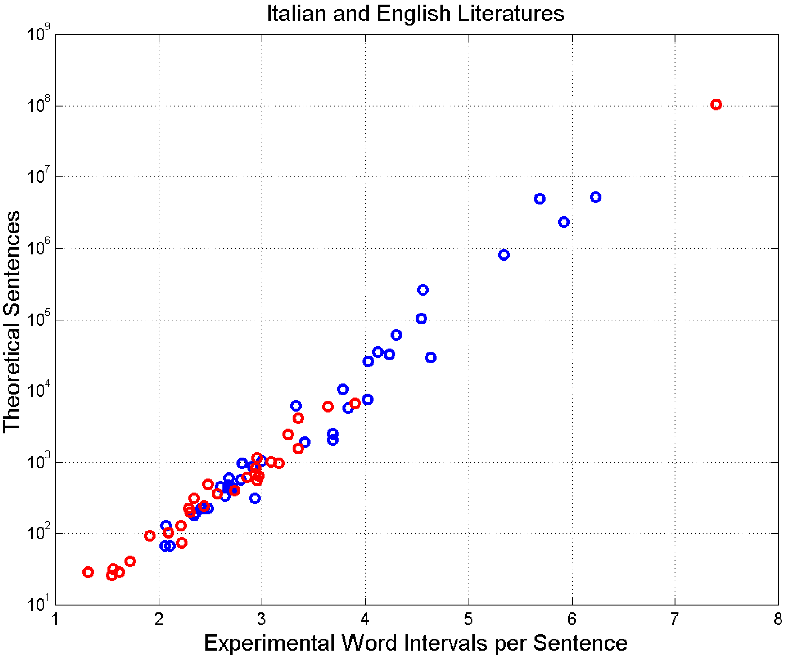
By referring to Figure 7, the interpolation between the integers of Table 2 to find the curve of constant

C_{F}

—given by the real number

<M_{F}>

—is linear along both axes. At the intersection of the vertical line (corresponding to the real number

<P_{F}>

) and the new curve (corresponding to the real number

<M_{F}>

), we find the theoretical

S_{W}^{(C_{F})}

by rounding the value to the nearest integer toward zero. For example, for David Copperfield, in Table A2 we read

S_{P_{F}}^{(M_{F})} = 19,610

, and the interpolation gives

S_{W}^{(C_{F})} = 1553

. Figure 9 shows the result of this exercise. We see that

S_{W}^{(C_{F})}

increases rapidly with

<M_{F}>

. The most displaced (red) circle is due to Robinson Crusoe.

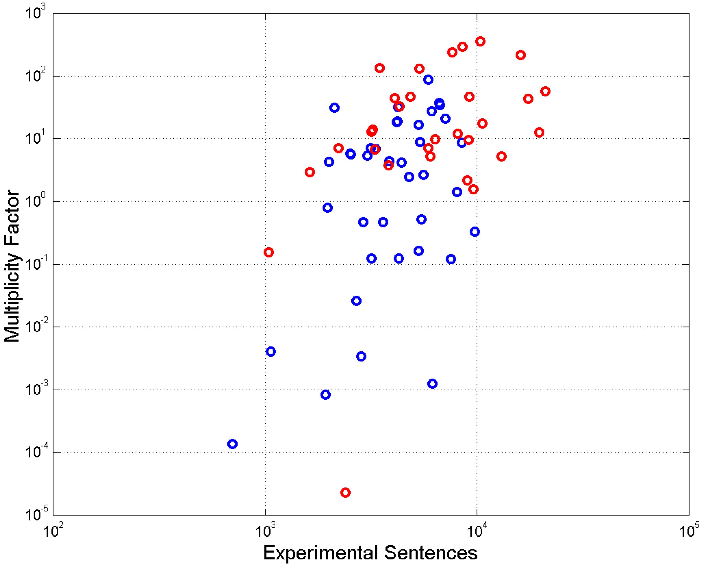
The comparison between

S_{P_{F}}^{(M_{F})}

and

S_{W}^{(C_{F})}

is performed by defining a multiplicity factor

α

, defined as the ratio between

S_{P_{F}}^{(M_{F})}

(experimental value) and

S_{W}^{(C_{F})}

(theoretical value):

α = \frac{S_{P_{F}}^{(M_{F})}}{S_{W}^{(C_{F})}}

(9)

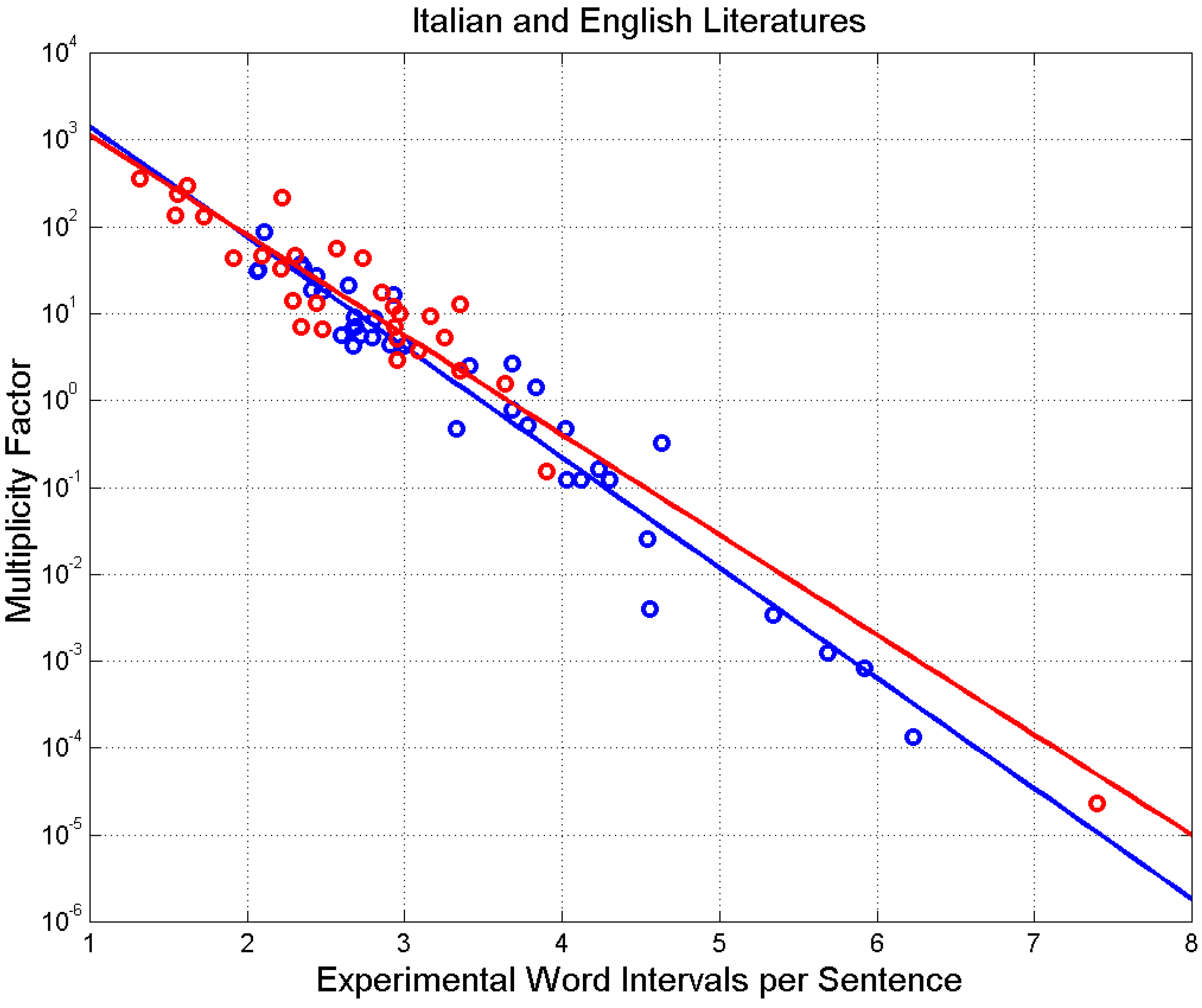
The values of

α

for each novel are reported in Table A1 and Table A2. For example, for David Copperfield,

α = 19,610 / 1553 = 12.63

. Figure 10 shows

α

versus

S_{P_{F}}^{(M_{F})}

. We notice a fairly significant increasing trend of

α

with

S_{P_{F}}^{(M_{F})}

.

Figure 11 shows

α

versus

S_{W}^{(C_{F})}

. An inverse relation power law is a good fit:

α = 3886 / S_{W}^{(C_{F})} Italian

(10)

α = 6028 / S_{W}^{(C_{F})} English

(11)

The correlation coefficient of log values is

- 0.9873

for Italian and

- 0.9710

for English.

Based on Equations (10) and (11),

α = 1

when

S_{W}^{(C_{F})} = 3886

for Italian novels and

S_{W}^{(C_{F})} = 6028

for English novels; therefore, novels with sentences in the range

4000 ~ 6000

use, on average, the number of sentences theoretically available for their averages

<P_{F}>

and

<M_{F}>

.

Figure 12 shows

α

versus

< M_{F} >

. In this case, an exponential law is a good fit:

α = 26,027 \times e^{- 2.923 \times M_{F}} Italian

(12)

α = 15,855 \times e^{- 2.649 \times M_{F}} English

(13)

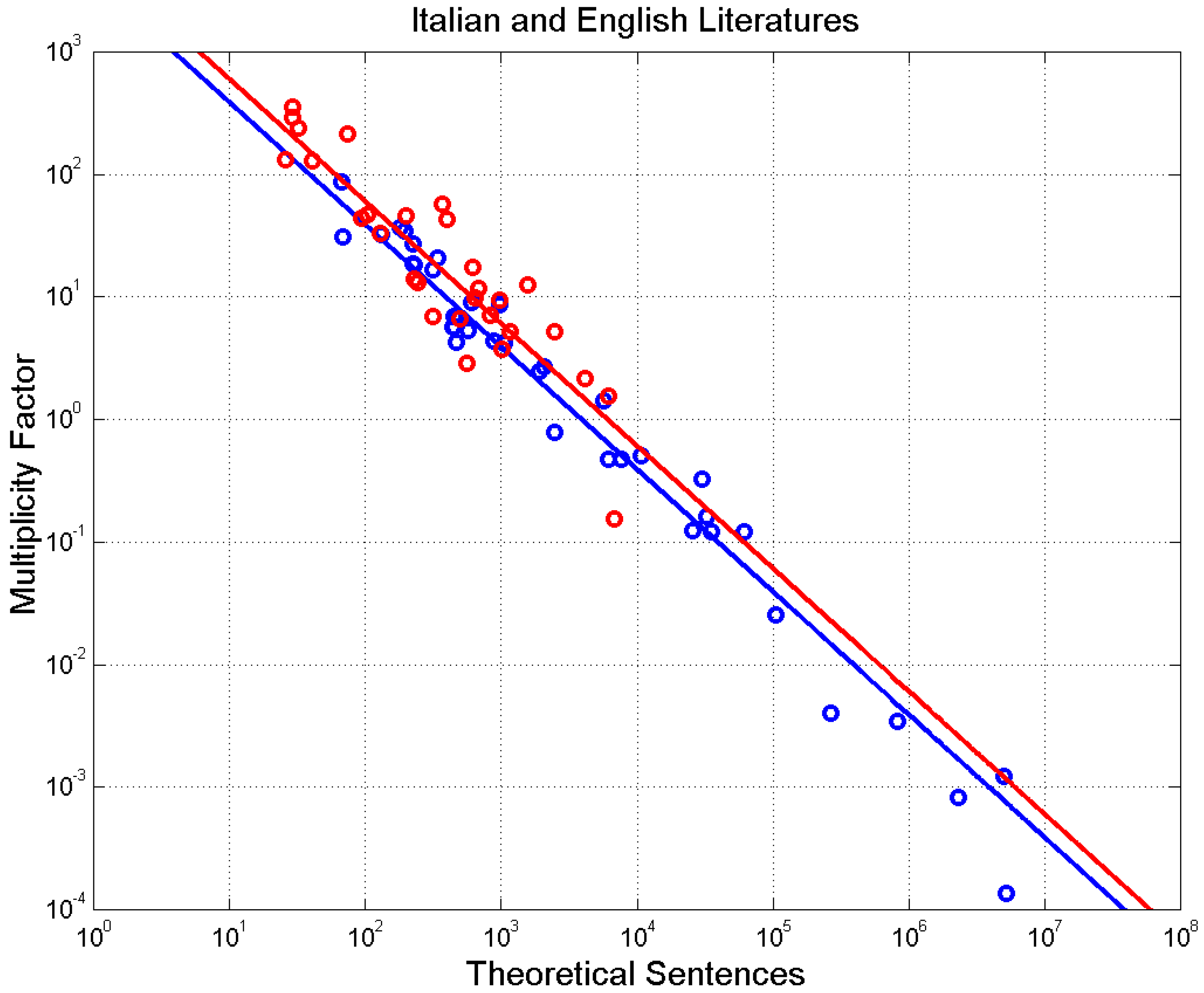
For the Italian literature in question, (correlation coefficient of linear–log values is

- 0.9697

)

α = 1

when

M_{F} = 3.48

; for the English literature (correlation coefficient of linear–log values is

- 0.9603

),

α = 1

when

M_{F} = 3.65

. Therefore, novels with sentences in the range

4000 ~ 6000

use, on average, the same E–STM buffer size of

M_{F} \approx 3.5

cells.

From Figure 10, Figure 11 and Figure 12, we can draw the following conclusion: in general,

α > 1

is more likely than

α < 1

and often

α ≫ 1

. When

α ≫ 1

, the writer reuses the same pattern of number of words many times. The multiplicity factor, therefore, indicates also the minimum multiplicity of meaning conveyed by an E–STM besides, of course, the many diverse meanings conveyed by the same sequence of

I_{p} s

obtainable by only changing words. Few novels show

α < 1

. In these cases, the writer has enough diverse patterns to convey meaning, but most of them are not used.

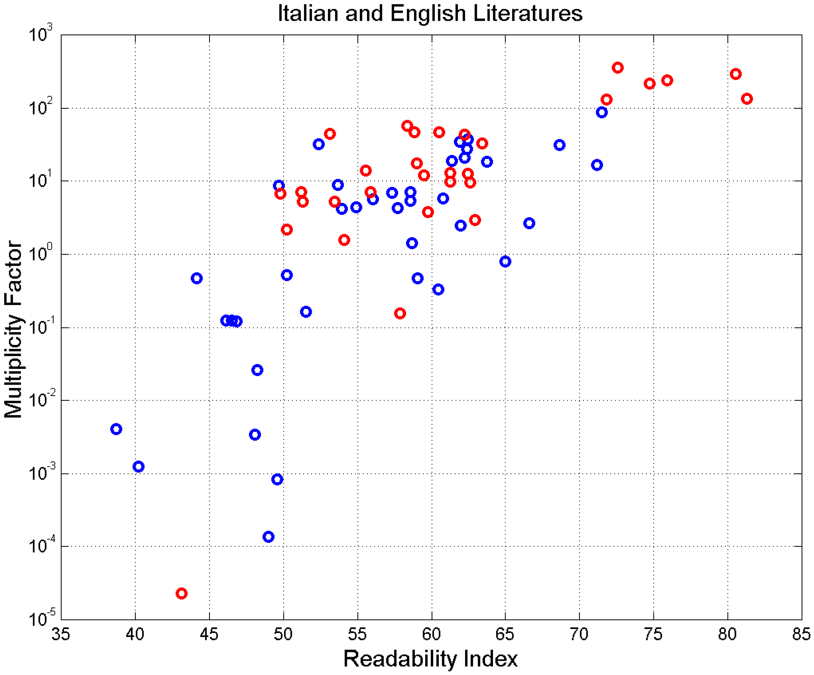
Finally, it is interesting to relate

α

to a universal readability factor

G_{U}

, which is a function of both

P_{F}

and

I_{P}

[43].

The universal readability index, as compared to the current readability indices for the few languages for which they are available (mainly for English [43]), considers also the reader’s short-term memory processing capacity. It can be used to assess the readability of texts written in any alphabetical language, as described in [43].

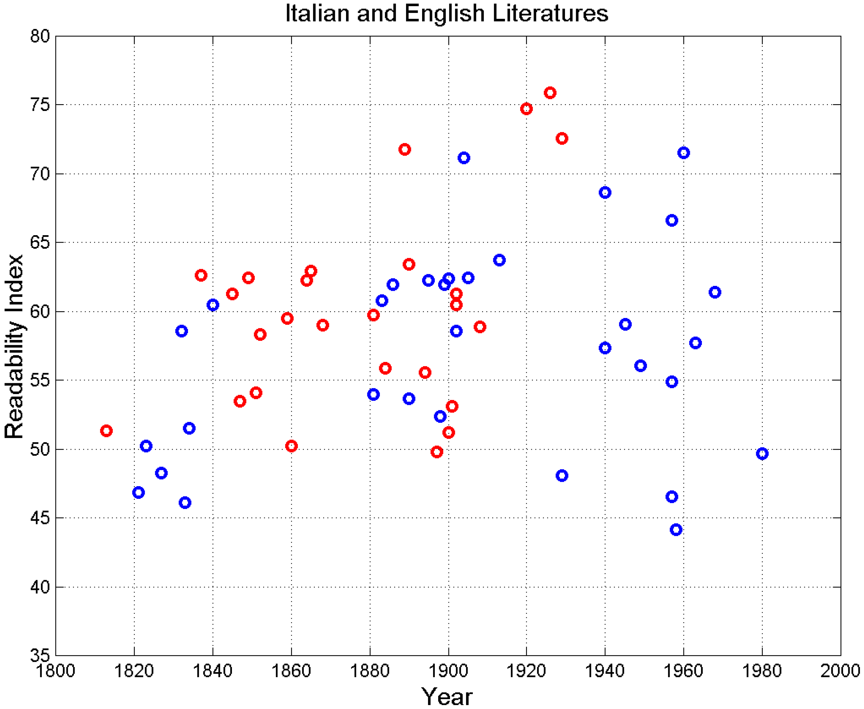
Figure 13 shows

α

versus

G_{U}

. Because the readability of a text increases as

G_{U}

increases, we can see that the novels with

α < 1

tend to be less readable than those with

α > 1

. The less-readable novels have, in general, large values of

<P_{F}>

and therefore may contain more E–STM cells (large

<M_{F}>

).

In conclusion, if a writer does use the full variety of sentence patterns available, or even overuses them, then he/she writes texts that are easier to read. On the other hand, if a writer does not use the full variety of sentence patterns available, then he/she tends to write texts that are more difficult to read. In the next section, we define a useful index, the mismatch index, which describes these cases.

5. Mismatch Index

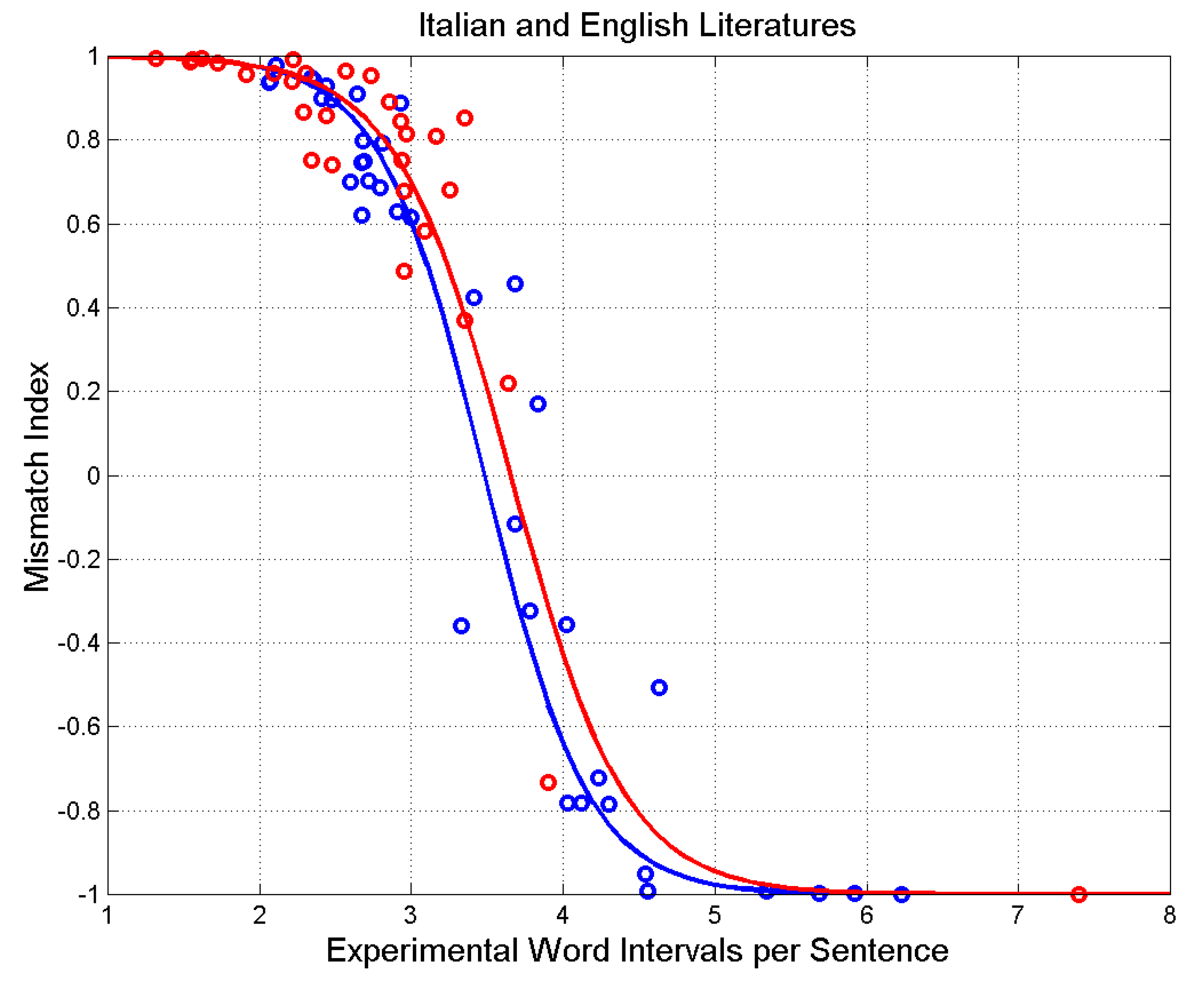
We define a useful index, the mismatch index, which measures to what extent a writer uses the number of sentences that are theoretically available according to the averages

<P_{F}>

and

<M_{F}>

of the novel. For this purpose, we define the mismatch index:

I_{M} = \frac{S_{P_{F}}^{(M_{F})} - S_{W}^{(C_{F})}}{S_{P_{F}}^{(M_{F})} + S_{W}^{(C_{F})}} = \frac{α - 1}{α + 1}

(14)

According to Equation (14),

I_{M} = 0

when

S_{P_{F}}^{(M_{F})} = S_{W}^{(C_{F})}

; hence,

α = 1,

and in this case the experiment and theory are perfectly matched. They are overmatched when

I_{M} > 0

(

α > 1)

and undermatched when

I_{M} < 0

(

α < 1)

.

Figure 14 shows the scatterplot of

I_{M}

versus

M_{F}

. The mathematical models drawn are calculated by substituting Equations (12) and (13) in Equation (14). We can reiterate that when

I_{M} > 0

(overmatching,

M_{F} ≲ 3.5

), the writer repeats sentence patterns because there are not enough diverse patterns to convey all the meanings. The texts are easier to read. When

I_{M} < 0

(undermatching,

M_{F} ≳ 3.5

), the writer has theoretically many sentence patterns to choose from, but he/she uses only a few or very few of them. The texts are more difficult to read.

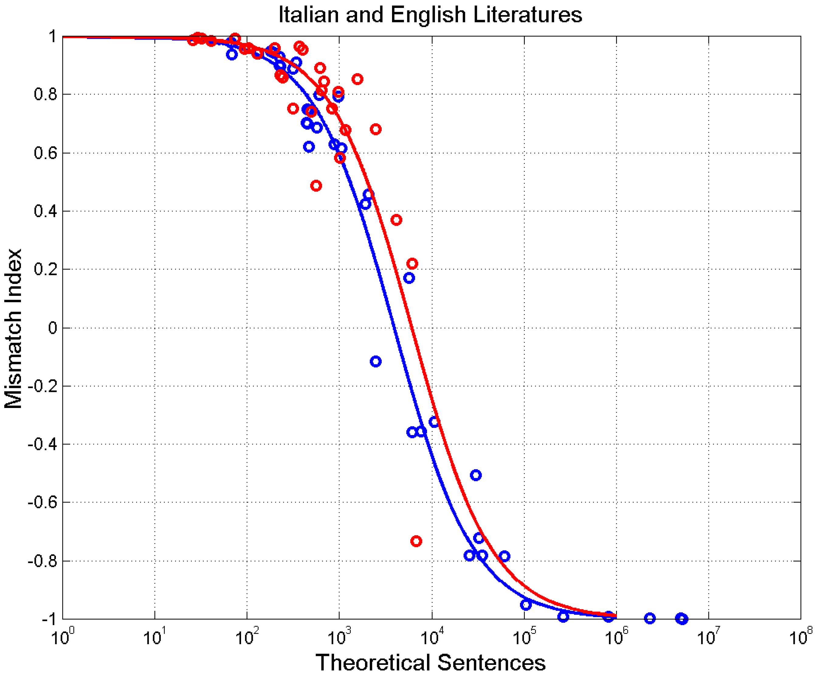
Figure 15 shows the scatterplot of

I_{M}

versus

S_{W}^{(C_{F})}

. The mathematical models drawn were calculated by substituting Equations (10) and (11) in Equation (14). Overmatching was found for

S_{W}^{(C_{F})} < 3886

for Italian and

S_{W}^{(C_{F})} < 6028

for English.

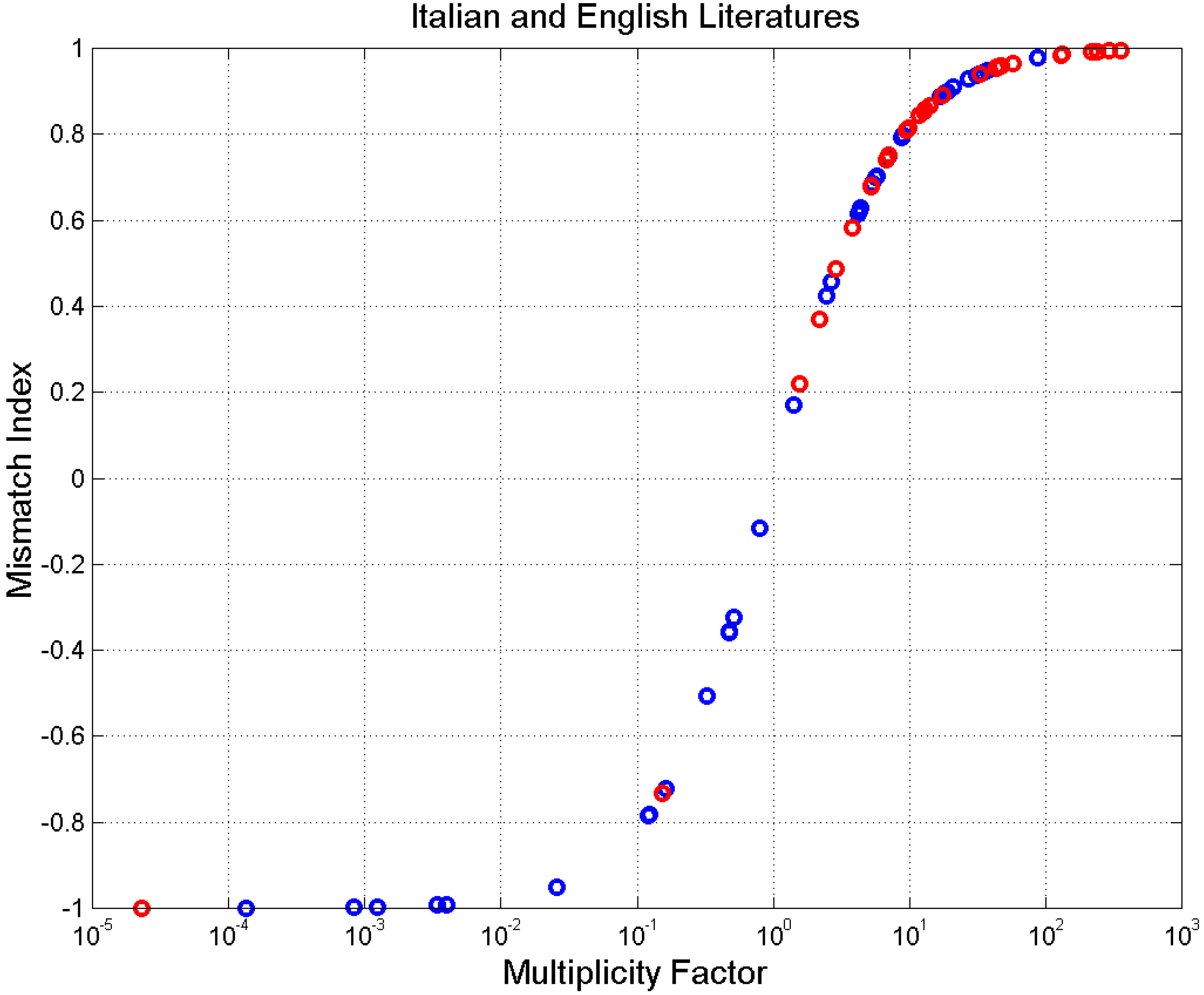
Finally, Figure 16 shows

I_{M}

versus

α

, Equation (14), a picture that summarizes the entire analysis of mismatch.

As we can see by reading the years of publication in Table A1 and Table A2, the novels span a long period. Do the parameters studied depend on time? In the next section, we show that the answer to this question is positive.

6. Time Dependence

The novels considered in Table A1 and Table A2 were published in a period spanning several centuries. We show that the multiplicity factor

α

and the mismatch index

I_{M}

do depend on time.

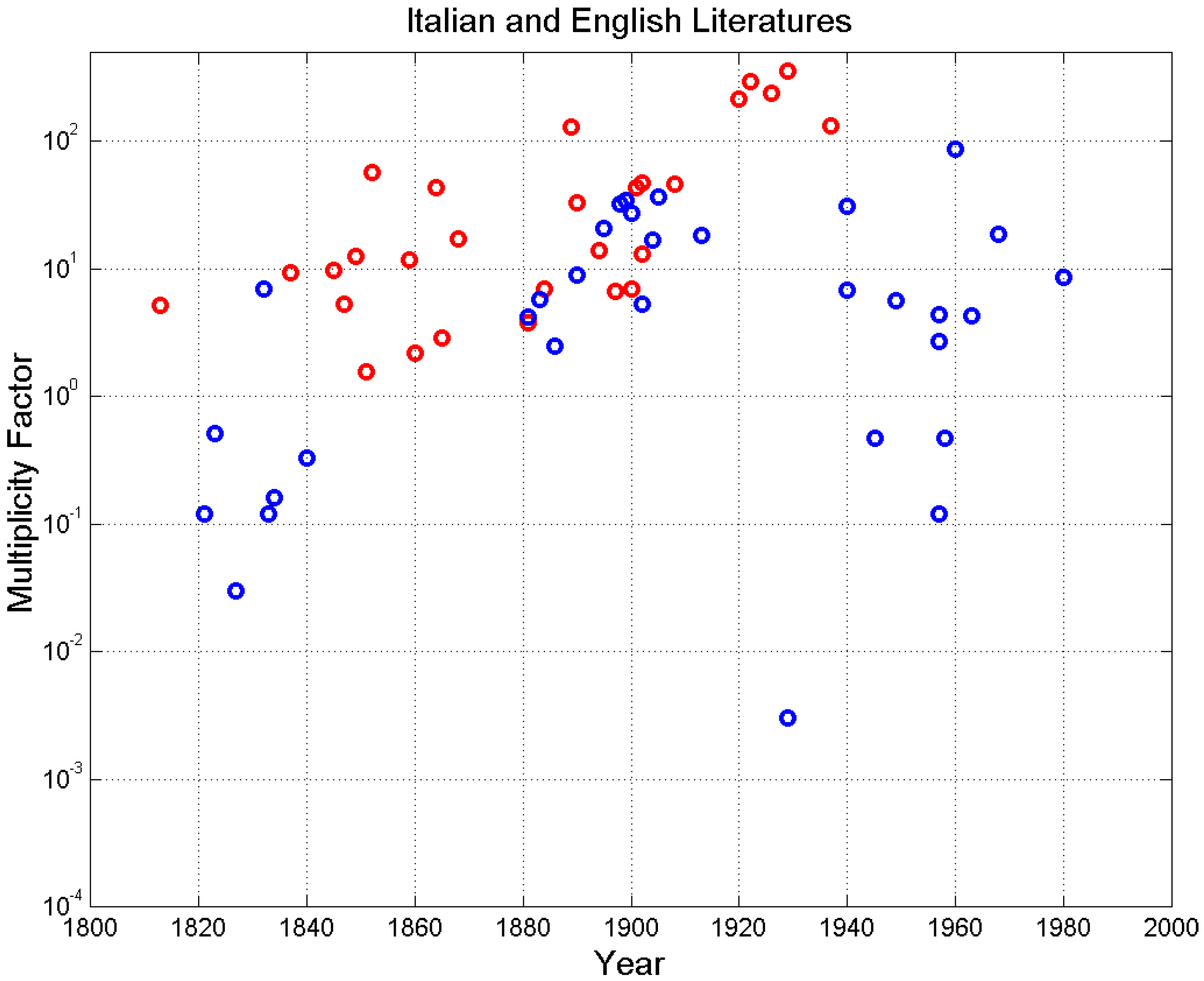
Figure 17 shows the multiplicity factors versus the years of publication of the novels since 1800. It is evident that writers tend to use larger values of

α

—therefore the E–STM buffers are of smaller sizes—as we approach the present epoch and a possible saturation at

α \approx 100

. The English literature shows a stable increasing pattern while the Italian literature seems to contain samples that come from two diverse sets of data, one of which evolved in agreement with English literature, the other (given by the novels labelled with “*” in Table A1) is always increasing with time but with a diverse slope.

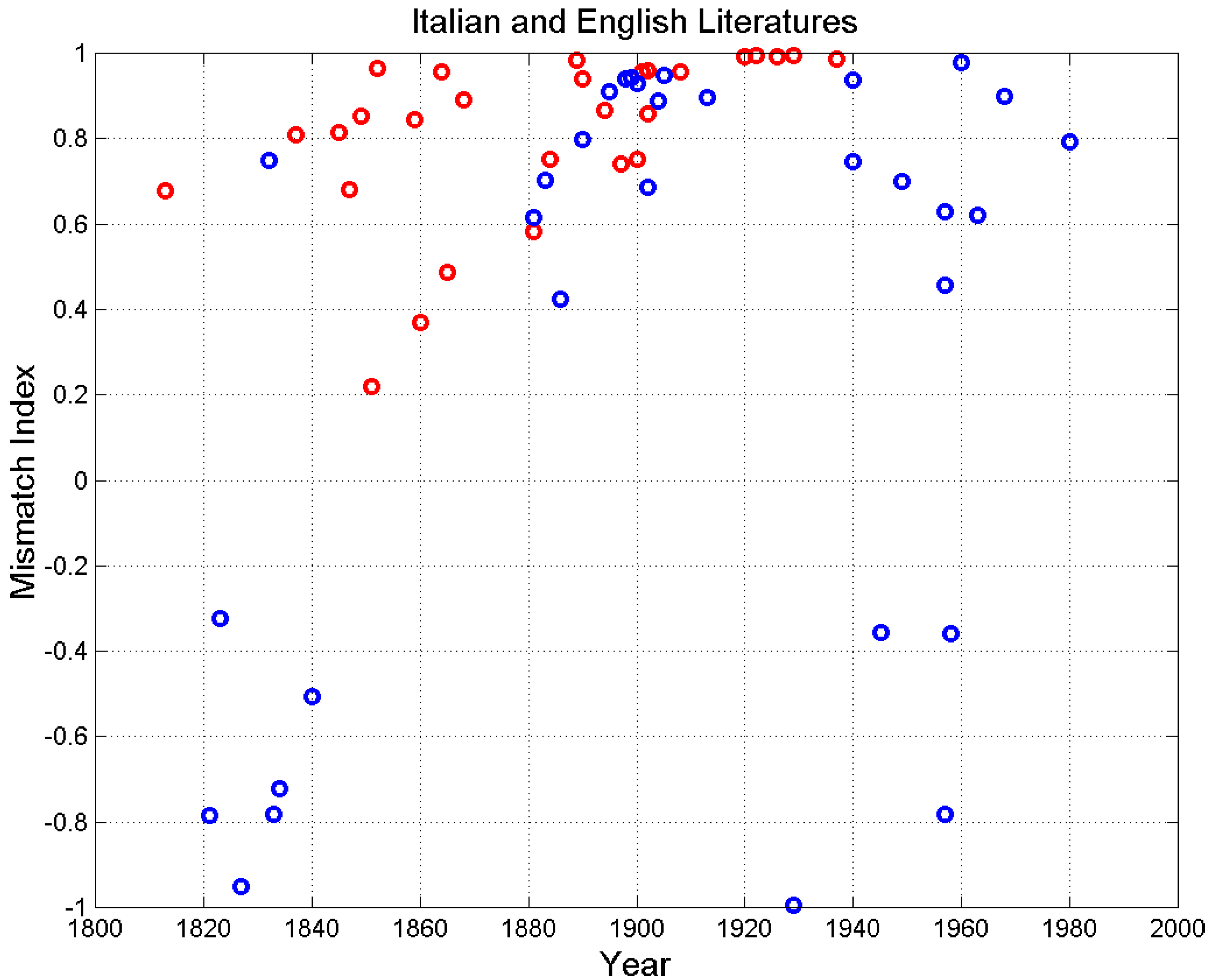
Figure 18 shows the mismatch index versus the year of novel publication.

Figure 19 shows the universal readability index versus time. In both Figure 18 and Figure 19, we can observe the same trends shown in Figure 17, which therefore reinforces the conjecture that: (a) the writers are partially changing their style with time by making their novels more readable, i.e., more matched to less-educated readers according to the relationship between

G_{U}

and the schooling years in the Italian school system, as discussed in [43]; (b) a saturation seems to occur in all parameters in the novels written in the second half of the XX century, at least according to the novels of Appendix B.

7. Summary and Future Work

In the present paper, we have further investigated the mathematical structure of sentences and its connections with human short–term memory. This structure is defined by two independent variables which apparently engage two short-term memory buffers in series. The first buffer is modelled according to the number of words between two consecutive interpunctions—variable-termed word interval

I_{P}

—which follows Miller’s

7 \pm 2

law; the second buffer is modelled by the number of word intervals contained in a sentence,

M_{F}

, ranging approximately from one to seven. These values arise from an extensive analysis of alphabetical texts [44].

We have studied the numerical patterns (combinations of

I_{P}

and

M_{F}

) that determine the number of sentences that theoretically can be recorded in the two memory buffers—which increases with

I_{P}

and

M_{F}

—and we have compared the theoretical results with those that are actually found in novels from Italian and English literature. We have found that most writers, in both languages, write for readers with small memory buffers and, consequently, are forced to reuse sentence patterns to convey multiple meanings. In this case, texts are easier to read, according to the universal readability index.

Future work should consider other literatures to confirm what, in our opinion, is general because the topic is connected to the human mind. The same analysis performed on ancient languages, such as Greek and Latin—for which there are large literary corpora—would show whether these ancient writers/readers displayed similar short–term memory buffers.

Funding

This research received no external funding.

Institutional Review Board Statement

Not applicable.

Informed Consent Statement

Not applicable.

Data Availability Statement

Data are contained within the article.

Acknowledgments

The author wishes to thank the many scholars who, with great care and love, maintain digital texts to be available to readers and scholars of different academic disciplines, such as Perseus Digital Library and Project Gutenberg.

Conflicts of Interest

The author declares no conflicts of interest.

Appendix A. List of Mathematical Symbols

Symbol	Definition
$C_{F}$	Cells of E–STM buffer
$G_{U}$	Universal readability index
$I_{M}$	Mismatch index
$I_{p}$	Word interval
$M_{F}$	Word intervals in a sentence, chapter average
$<M_{F}>$	Word intervals in a sentence, novel average
$P_{F}$	Words in a sentence, chapter average
$< P_{F} >$	Words in a sentence, novel average
$S_{P_{F}}^{(M_{F})}$	Experimental sentences
$S_{W}^{(C_{F})}$	Theoretical sentences written in $C_{F}$ cells
$W$	Words in a sentence
$f (x)$	Three–parameter log–normal density function
$f_{C_{F}} (x)$	Gaussian PDF
$m_{C_{F}}$	Mean value of Gaussian PDF
$s_{C_{F}}$	standard deviation of Gaussian PDF
$α$	Multiplicity factor
$ε$	Efficiency factor
$μ_{x}$	Mean value of log–normal PDF
$σ_{x}$	standard deviation of log–normal PDF

Appendix B. List of the Novels Considered from Italian and English Literature

Table A1 and Table A2 list the authors, the titles of the novels, and their years of publication in either Italian and English literature as considered in the paper, with deep–language average statistics, multiplicity factor

α

, and mismatch index

I_{M}

. The averages

< C_{P} >, < P_{F} >, < I_{P} >

< M_{F} >

have been calculated by weighting each chapter value with its fraction of the total number of words in the novel, as described in [32].

Table A1. Authors of novels of Italian literature. Number of total sentences (sentences ending with full stops, question marks, or exclamation marks); average number of characters per word,

< C_{P} >

; average number of words pr sentence,

< P_{F} >

; average number of word intervals,

< I_{P} >

; average number word intervals per sentence,

< M_{F} >

; multiplicity factor

α

; and mismatch index

I_{M}

.

Table A1. Authors of novels of Italian literature. Number of total sentences (sentences ending with full stops, question marks, or exclamation marks); average number of characters per word,

< C_{P} >

; average number of words pr sentence,

< P_{F} >

; average number of word intervals,

< I_{P} >

; average number word intervals per sentence,

< M_{F} >

; multiplicity factor

α

; and mismatch index

I_{M}

.

Author (Literary Work, Year)	Sentences	$< C_{P} >$	$< P_{F} >$	$< I_{P} >$	$< M_{F} >$	$α$	$I_{M}$
Anonymous (I Fioretti di San Francesco, 1476)	1064	4.65	37.70	8.24	4.56	0.004	−0.99
Bembo Pietro (Prose, 1525)	1925	4.37	37.91	6.42	5.92	0.001	−1.00
Boccaccio Giovanni (Decameron, 1353)	6147	4.48	44.27	7.79	5.69	0.001	−1.00
Buzzati Dino (Il deserto dei tartari, 1940)	3311	5.10	17.75	6.63	2.67	6.90	0.75
Buzzati Dino (La boutique del mistero, 1968 *)	4219	4.82	15.45	6.37	2.41	18.83	0.90
Calvino (Il barone rampante, 1957 *)	3864	4.63	19.87	6.73	2.91	4.37	0.63
Calvino Italo (Marcovaldo, 1963 *)	2000	4.74	17.60	6.59	2.67	4.28	0.62
Cassola Carlo (La ragazza di Bube, 1960 *)	5873	4.48	11.93	5.64	2.11	87.66	0.98
Collodi Carlo (Pinocchio, 1883)	2512	4.60	16.92	6.19	2.72	5.74	0.70
Da Ponte Lorenzo (Vita, 1823)	5459	4.71	26.15	6.91	3.78	0.51	−0.32
Deledda Grazia (Canne al vento, 1913, Nobel Prize 1926)	4184	4.51	15.08	6.06	2.48	18.35	0.90
D’Azeglio Massimo (Ettore Fieramosca, 1833)	3182	4.64	29.77	7.36	4.03	0.12	−0.78
De Amicis Edmondo (Cuore, 1886)	4775	4.55	19.43	5.61	3.41	2.48	0.42
De Marchi Emilio (Demetrio Panelli, 1890)	5363	4.70	18.95	7.06	2.68	8.95	0.80
D’Annunzio Gabriele (Le novelle delle Pescara, 1902)	3027	4.91	17.99	6.38	2.79	5.35	0.68
Eco Umberto (Il nome della rosa, 1980 *)	8490	4.81	21.08	7.46	2.81	8.70	0.79
Fogazzaro (Il santo, 1905)	6637	4.79	14.84	6.33	2.34	37.08	0.95
Fogazzaro (Piccolo mondo antico, 1895)	7069	4.79	16.08	6.10	2.64	20.98	0.91
Gadda (Quer pasticciaccio brutto… 1957 *)	5596	4.76	18.43	4.98	3.68	2.69	0.46
Grossi Tommaso (Marco Visconti, 1834)	5301	4.59	28.07	6.56	4.23	0.16	−0.72
Leopardi Giacomo (Operette morali, 1827)	2694	4.70	31.78	6.90	4.54	0.03	−0.95
Levi Primo (Cristo si è fermato a Eboli, 1945 *)	3611	4.73	22.94	5.70	4.02	0.47	−0.36
Machiavelli Niccolò (Il principe, 1532)	702	4.71	40.17	6.45	6.23	0.0001	−1.00
Manzoni Alessandro (I promessi sposi, 1840)	9766	4.60	24.83	5.30	4.63	0.33	−0.51
Manzoni Alessandro (Fermo e Lucia, 1821)	7496	4.75	30.98	7.17	4.30	0.12	−0.78
Moravia Alberto (Gli indifferenti, 1929 *)	2830	4.81	36.00	6.74	5.34	0.003	−0.99
Moravia Alberto (La ciociara, 1957 *)	4271	4.56	29.93	7.28	4.12	0.12	−0.78
Pavese Cesare (La bella estate, 1940)	2121	4.54	12.37	5.97	2.06	31.19	0.94
Pavese Cesare (La luna e i falò, 1949 *)	2544	4.47	17.83	6.83	2.60	5.64	0.70
Pellico Silvio (Le mie prigioni, 1832)	3148	4.80	17.27	6.50	2.69	7.00	0.75
Pirandello Luigi (Il fu Mattia Pascal, 1904, Nobel Prize 1934)	5284	4.63	14.57	4.94	2.93	16.72	0.89
Sacchetti Franco (Trecentonovelle, 1392)	8060	4.37	22.43	5.82	3.83	1.41	0.17
Salernitano Masuccio (Il Novellino, 1525)	1965	4.40	19.20	5.14	3.68	0.79	−0.12
Salgari Emilio (Il corsaro nero, 1899)	6686	4.99	15.09	6.36	2.36	34.46	0.94
Salgari Emilio (I minatori dell’Alaska, 1900)	6094	5.01	15.24	6.25	2.44	27.21	0.93
Svevo Italo (Senilità, 1898)	4236	4.86	16.04	7.75	2.07	32.34	0.94
Tomasi di Lampedusa (Il gattopardo, 1958 *)	2893	4.99	26.42	7.90	3.33	0.47	−0.36
Verga (I Malavoglia, 1881)	4401	4.46	20.45	6.82	3.00	4.21	0.62

Table A2. Authors of the novels of English literature. Number of total sentences; average number of characters per word,

< C_{P} >

; average number of words pr sentence,

< P_{F} >

; average number of word intervals,

< I_{P} >

; average number word intervals per sentence,

< M_{F} >

; multiplicity factor

α

; and mismatch index

I_{M}

. Notice that for Dickens’ novels, Table 1 of [45] reported the number of sentences ending only with full stops; sentences ending with question marks and exclamation marks were not reported, contrarily to all other literary texts there reported. Moreover, the analysis conducted in [45] was performed by considering only the sentences ending with full stops; this is why the values of

<P_{F}>

and

<M_{F}>

there reported are larger (upper bounds) than those listed below.

Table A2. Authors of the novels of English literature. Number of total sentences; average number of characters per word,

< C_{P} >

; average number of words pr sentence,

< P_{F} >

; average number of word intervals,

< I_{P} >

; average number word intervals per sentence,

< M_{F} >

; multiplicity factor

α

; and mismatch index

I_{M}

. Notice that for Dickens’ novels, Table 1 of [45] reported the number of sentences ending only with full stops; sentences ending with question marks and exclamation marks were not reported, contrarily to all other literary texts there reported. Moreover, the analysis conducted in [45] was performed by considering only the sentences ending with full stops; this is why the values of

<P_{F}>

and

<M_{F}>

there reported are larger (upper bounds) than those listed below.

Literary Work (Author, Year)	Sentences	$< C_{P} >$	$<P_{F}>$	$< I_{P} >$	$<M_{F}>$	$α$	$I_{M}$
The Adventures of Oliver Twist (C. Dickens, 1837–1839)	9121	4.23	18.04	5.70	3.16	9.46	0.81
David Copperfield (C. Dickens, 1849–1850)	19,610	4.04	18.83	5.61	3.35	12.63	0.85
Bleak House (C. Dickens, 1852–1853)	20,967	4.23	16.95	6.59	2.57	56.98	0.97
A Tale of Two Cities (C. Dickens, 1859)	8098	4.26	18.27	6.19	2.93	11.89	0.84
Our Mutual Friend (C. Dickens, 1864–1865)	17,409	4.22	16.46	6.03	2.73	43.41	0.95
Matthew King James (1611)	1040	4.27	22.96	5.90	3.90	0.15	−0.73
Robinson Crusoe (D. Defoe, 1719)	2393	3.94	52.90	7.12	7.40	0.00002	−1.00
Pride and Prejudice (J. Austen, 1813)	6013	4.40	21.31	7.16	2.95	5.20	0.68
Wuthering Heights (E. Brontë, 1845–1846)	6352	4.27	17.78	5.97	2.97	9.83	0.82
Vanity Fair (W. Thackeray, 1847–1848)	13,007	4.63	21.95	6.73	3.25	5.26	0.68
Moby Dick (H. Melville, 1851)	9582	4.52	23.82	6.45	3.64	1.56	0.22
The Mill On The Floss (G. Eliot, 1860)	9018	4.29	23.84	7.09	3.35	2.17	0.37
Alice’s Adventures in Wonderland (L. Carroll, 1865)	1629	3.96	17.19	5.79	2.95	2.90	0.49
Little Women (L.M. Alcott, 1868–1869)	10,593	4.18	18.09	6.30	2.85	17.34	0.89
Treasure Island (R. L. Stevenson, 1881–1882)	3824	4.02	18.93	6.05	3.09	3.79	0.58
Adventures of Huckleberry Finn (M. Twain, 1884)	5887	3.85	19.39	6.63	2.94	7.05	0.75
Three Men in a Boat (J.K. Jerome, 1889)	5341	4.25	10.55	6.14	1.72	130.27	0.98
The Picture of Dorian Gray (O. Wilde, 1890)	4292	4.19	14.30	6.29	2.21	33.02	0.94
The Jungle Book (R. Kipling, 1894)	3214	4.11	16.46	7.14	2.29	14.10	0.87
The War of the Worlds (H.G. Wells, 1897)	3306	4.38	19.22	7.67	2.48	6.72	0.74
The Wonderful Wizard of Oz (L.F. Baum, 1900)	2219	4.017	17.90	7.63	2.34	7.02	0.75
The Hound of The Baskervilles (A.C. Doyle, 1901–1902)	4080	4.15	15.07	7.83	1.91	43.87	0.96
Peter Pan (J.M. Barrie, 1902)	3177	4.12	15.65	6.35	2.44	13.07	0.86
A Little Princess (F.H. Burnett, 1902–1905)	4838	4.18	14.26	6.79	2.09	46.97	0.96
Martin Eden (J. London, 1908–1909)	9173	4.32	15.61	6.76	2.30	46.33	0.96
Women in love (D.H. Lawrence, 1920)	16,048	4.26	11.62	5.22	2.22	216.86	0.99
The Secret Adversary (A. Christie, 1922)	8536	4.28	8.97	5.52	1.62	294.34	0.99
The Sun Also Rises (E. Hemingway, 1926)	7614	3.92	9.43	6.02	1.56	237.94	0.99
A Farewell to Arms (H. Hemingway,1929)	10,324	3.94	9.05	6.80	1.32	356.00	0.99
Of Mice and Men (J. Steinbeck, 1937)	3463	4.02	8.63	5.61	1.54	133.19	0.99

References

Matricciani, E. Is Short-Term Memory Made of Two Processing Units? Clues from Italian and English Literatures down Several Centuries. Information 2024, 15, 6. [Google Scholar] [CrossRef]
Deniz, F.; Nunez-Elizalde, A.O.; Huth, A.G.; Gallant Jack, L. The Representation of Semantic Information Across Human Cerebral Cortex During Listening Versus Reading Is Invariant to Stimulus Modality. J. Neurosci. 2019, 39, 7722–7736. [Google Scholar] [CrossRef]
Miller, G.A. The magical number seven, plus or minus two: Some limits on our capacity for processing information. Psychol. Rev. 1956, 63, 81–97. [Google Scholar] [CrossRef]
Crowder, R.G. Short-term memory: Where do we stand? Mem. Cogn. 1993, 21, 142–145. [Google Scholar] [CrossRef]
Lisman, J.E.; Idiart, M.A.P. Storage of 7 ± 2 Short-Term Memories in Oscillatory Subcycles. Science 1995, 267, 1512–1515. [Google Scholar] [CrossRef]
Cowan, N. The magical number 4 in short-term memory: A reconsideration of mental storage capacity. Behav. Brain Sci. 2001, 24, 87–114. [Google Scholar] [CrossRef]
Bachelder, B.L. The Magical Number 7 ± 2: Span Theory on Capacity Limitations. Behav. Brain Sci. 2001, 24, 116–117. [Google Scholar] [CrossRef]
Saaty, T.L.; Ozdemir, M.S. Why the Magic Number Seven Plus or Minus Two. Math. Comput. Model. 2003, 38, 233–244. [Google Scholar] [CrossRef]
Burgess, N.; Hitch, G.J. A revised model of short-term memory and long-term learning of verbal sequences. J. Mem. Lang. 2006, 55, 627–652. [Google Scholar] [CrossRef]
Richardson, J.T.E. Measures of short-term memory: A historical review. Cortex 2007, 43, 635–650. [Google Scholar] [CrossRef]
Mathy, F.; Feldman, J. What’s magic about magic numbers? Chunking and data compression in short-term memory. Cognition 2012, 122, 346–362. [Google Scholar] [CrossRef] [PubMed]
Gignac, G.E. The Magical Numbers 7 and 4 Are Resistant to the Flynn Effect: No Evidence for Increases in Forward or Backward Recall across 85 Years of Data. Intelligence 2015, 48, 85–95. [Google Scholar] [CrossRef]
Trauzettel-Klosinski, S.; Dietz, K. Standardized Assessment of Reading Performance: The New International Reading Speed Texts IreST. Investig. Ophthalmol. Vis. Sci. 2012, 53, 5452–5461. [Google Scholar] [CrossRef] [PubMed]
Melton, A.W. Implications of Short-Term Memory for a General Theory of Memory. J. Verbal Learn. Verbal Behav. 1963, 2, 1–21. [Google Scholar] [CrossRef]
Atkinson, R.C.; Shiffrin, R.M. The Control of Short-Term Memory. Sci. Am. 1971, 225, 82–91. [Google Scholar] [CrossRef]
Murdock, B.B. Short-Term Memory. Psychol. Learn. Motiv. 1972, 5, 67–127. [Google Scholar]
Baddeley, A.D.; Thomson, N.; Buchanan, M. Word Length and the Structure of Short-Term Memory. J. Verbal Learn. Verbal Behav. 1975, 14, 575–589. [Google Scholar] [CrossRef]
Case, R.; Midian Kurland, D.; Goldberg, J. Operational efficiency and the growth of short-term memory span. J. Exp. Child Psychol. 1982, 33, 386–404. [Google Scholar] [CrossRef]
Grondin, S. A temporal account of the limited processing capacity. Behav. Brain Sci. 2000, 24, 122–123. [Google Scholar] [CrossRef]
Pothos, E.M.; Joula, P. Linguistic structure and short-term memory. Behav. Brain Sci. 2000, 138–139. [Google Scholar] [CrossRef]
Conway, A.R.A.; Cowan, N.; Michael, F.; Bunting, M.F.; Therriaulta, D.J.; Minkoff, S.R.B. A latent variable analysis of working memory capacity, short-term memory capacity, processing speed, and general fluid intelligence. Intelligence 2002, 30, 163–183. [Google Scholar] [CrossRef]
Jonides, J.; Lewis, R.L.; Nee, D.E.; Lustig, C.A.; Berman, M.G.; Moore, K.S. The Mind and Brain of Short-Term Memory. Annu. Rev. Psychol. 2008, 69, 193–224. [Google Scholar] [CrossRef] [PubMed]
Barrouillest, P.; Camos, V. As Time Goes by: Temporal Constraints in Working Memory. Curr. Dir. Psychol. Sci. 2012, 21, 413–419. [Google Scholar] [CrossRef]
Potter, M.C. Conceptual short term memory in perception and thought. Front. Psychol. 2012, 3, 113. [Google Scholar] [CrossRef]
Jones, G.; Macken, B. Questioning short-term memory and its measurements: Why digit span measures long-term associative learning. Cognition 2015, 144, 1–13. [Google Scholar] [CrossRef] [PubMed]
Chekaf, M.; Cowan, N.; Mathy, F. Chunk formation in immediate memory and how it relates to data compression. Cognition 2016, 155, 96–107. [Google Scholar] [CrossRef]
Norris, D. Short-Term Memory and Long-Term Memory Are Still Different. Psychol. Bull. 2017, 143, 992–1009. [Google Scholar] [CrossRef]
Houdt, G.V.; Mosquera, C.; Napoles, G. A review on the long short-term memory model. Artif. Intell. Rev. 2020, 53, 5929–5955. [Google Scholar] [CrossRef]
Islam, M.; Sarkar, A.; Hossain, M.; Ahmed, M.; Ferdous, A. Prediction of Attention and Short-Term Memory Loss by EEG Workload Estimation. J. Biosci. Med. 2023, 11, 304–318. [Google Scholar] [CrossRef]
Rosenzweig, M.R.; Bennett, E.L.; Colombo, P.J.; Lee, P.D.W. Short-term, intermediate-term and Long-term memories. Behav. Brain Res. 1993, 57, 193–198. [Google Scholar] [CrossRef]
Kaminski, J. Intermediate-Term Memory as a Bridge between Working and Long-Term Memory. J. Neurosci. 2017, 37, 5045–5047. [Google Scholar] [CrossRef]
Matricciani, E. Deep Language Statistics of Italian throughout Seven Centuries of Literature and Empirical Connections with Miller’s 7 ∓ 2 Law and Short-Term Memory. Open J. Stat. 2019, 9, 373–406. [Google Scholar] [CrossRef]
Strinati, E.C.; Barbarossa, S. 6G Networks: Beyond Shannon towards Semantic and Goal-Oriented Communications. Comput. Netw. 2021, 190, 107930. [Google Scholar] [CrossRef]
Shi, G.; Xiao, Y.; Li, Y.; Xie, X. From semantic communication to semantic-aware networking: Model, architecture, and open problems. IEEE Commun. Mag. 2021, 59, 44–50. [Google Scholar] [CrossRef]
Xie, H.; Qin, Z.; Li, G.Y.; Juang, B.H. Deep learning enabled semantic communication systems. IEEE Trans. Signal Process. 2021, 69, 2663–2675. [Google Scholar] [CrossRef]
Luo, X.; Chen, H.H.; Guo, Q. Semantic communications: Overview, open issues, and future research directions. IEEE Wirel. Commun. 2022, 29, 210–219. [Google Scholar] [CrossRef]
Yang, W.; Du, H.; Liew, Z.Q.; Lim, W.Y.B.; Xiong, Z.; Niyato, D.; Chi, X.; Shen, X.; Miao, C. Semantic Communications for Future Internet: Fundamentals, Applications, and Challenges. IEEE Commun. Surv. Tutor. 2023, 25, 213–250. [Google Scholar] [CrossRef]
Xie, H.; Qin, A. A lite distributed semantic communication system for internet of things. IEEE J. Sel. Areas Commun. 2021, 39, 142–153. [Google Scholar]
Bellegarda, J.R. Exploiting Latent Semantic Information in Statistical Language Modeling. Proc. IEEE 2000, 88, 1279–1296. [Google Scholar] [CrossRef]
D’Alfonso, S. On Quantifying Semantic Information. Information 2011, 2, 61–101. [Google Scholar] [CrossRef]
Zhong, Y. A Theory of Semantic Information. China Commun. 2017, 14, 1–17. [Google Scholar] [CrossRef]
Papoulis Papoulis, A. Probability & Statistics; Prentice Hall: Hoboken, NJ, USA, 1990. [Google Scholar]
Matricciani, E. Readability Indices Do Not Say It All on a Text Readability. Analytics 2023, 2, 296–314. [Google Scholar] [CrossRef]
Matricciani, E. The Theory of Linguistic Channels in Alphabetical Texts; Cambridge Scholars Publishing: Newcastle upon Tyne, UK, 2024. [Google Scholar]
Matricciani, E. Capacity of Linguistic Communication Channels in Literary Texts: Application to Charles Dickens’ Novels. Information 2023, 14, 68. [Google Scholar] [CrossRef]

Figure 1. Flowchart of the two processing units of a sentence. The words

p_{1}

,

p_{2}

,…

p_{j}

are stored in the first buffer up to

j

items to complete a word interval

I_{P}

, which is approximately in Miller’s range, when an interpunction is introduced.

I_{P}

is then stored in the E–STM buffer, up to

k

items, i.e., in

M_{F}

cells, approximately one to six, until the sentence ends.

Figure 1. Flowchart of the two processing units of a sentence. The words

p_{1}

,

p_{2}

,…

p_{j}

are stored in the first buffer up to

j

items to complete a word interval

I_{P}

, which is approximately in Miller’s range, when an interpunction is introduced.

I_{P}

is then stored in the E–STM buffer, up to

k

items, i.e., in

M_{F}

cells, approximately one to six, until the sentence ends.

Figure 2. Conditional PDFs of words per sentence versus an E–STM buffer of

C_{F}

cells from two to eight. Each PDF can be modelled with a Gaussian PDF

f_{C_{F}} (x)

with a mean value proportional to

C_{F}

and a standard deviation proportional to

\sqrt{C_{F}}

.

Figure 2. Conditional PDFs of words per sentence versus an E–STM buffer of

C_{F}

cells from two to eight. Each PDF can be modelled with a Gaussian PDF

f_{C_{F}} (x)

with a mean value proportional to

C_{F}

and a standard deviation proportional to

\sqrt{C_{F}}

.

Figure 3. Conditional histograms of words per sentence versus an E–STM buffer of

C_{F}

cells from two to eight, obtained from Figure 1, by simulating 100,000 sentences weighted with the PDF of

M_{F}

.

Figure 3. Conditional histograms of words per sentence versus an E–STM buffer of

C_{F}

cells from two to eight, obtained from Figure 1, by simulating 100,000 sentences weighted with the PDF of

M_{F}

.

Figure 4. Scatterplot of

< P_{F} >

versus

< M_{F} >

of Italian novels (blue circles) and English novels (red circles).

Figure 4. Scatterplot of

< P_{F} >

versus

< M_{F} >

of Italian novels (blue circles) and English novels (red circles).

Figure 5. Overlap probability (%) versus

C_{F} - 1

(lower

C_{F}

);

p_{H L}

and

p_{L H}

are given by Equations (5) and (6).

Figure 5. Overlap probability (%) versus

C_{F} - 1

(lower

C_{F}

);

p_{H L}

and

p_{L H}

are given by Equations (5) and (6).

Figure 6. Number of sentences

S_{W}^{(C_{F})}

made of

W

words versus an E–STM buffer capacity of

C_{F}

.

Figure 6. Number of sentences

S_{W}^{(C_{F})}

made of

W

words versus an E–STM buffer capacity of

C_{F}

.

Figure 7. Number of sentences

S_{W}^{(C_{F})}

recordable in an E–STM buffer capacity of

C_{F}

versus words per sentence.

Figure 7. Number of sentences

S_{W}^{(C_{F})}

recordable in an E–STM buffer capacity of

C_{F}

versus words per sentence.

Figure 8. Efficiency

ε

, Equation (8), of an E–STM buffer of

C_{F}

cells versus words per sentence

W

.

Figure 8. Efficiency

ε

, Equation (8), of an E–STM buffer of

C_{F}

cells versus words per sentence

W

.

Figure 9. Theoretical number of sentences

S_{W}^{(C_{F})}

versus

<M_{F}>

for Italian (blue circles) and English (red circles) novels. The most displaced (red) circle is due to Robinson Crusoe.

Figure 9. Theoretical number of sentences

S_{W}^{(C_{F})}

versus

<M_{F}>

for Italian (blue circles) and English (red circles) novels. The most displaced (red) circle is due to Robinson Crusoe.

Figure 10. Multiplicity factor versus

S_{P_{F}}^{(M_{F})}

for Italian (blue circles) and English (red circles) novels.

Figure 10. Multiplicity factor versus

S_{P_{F}}^{(M_{F})}

for Italian (blue circles) and English (red circles) novels.

Figure 11. Multiplicity factor

α

versus theoretical number of words

S_{W}^{(C_{F})}

for Italian (blue circles and blue line) and English (red circles and red line) novels.

Figure 11. Multiplicity factor

α

versus theoretical number of words

S_{W}^{(C_{F})}

for Italian (blue circles and blue line) and English (red circles and red line) novels.

Figure 12. Multiplicity factor

α

versus

M_{F}

for Italian (blue circles and blue line) and English (red circles and red line) novels.

Figure 12. Multiplicity factor

α

versus

M_{F}

for Italian (blue circles and blue line) and English (red circles and red line) novels.

Figure 13. Multiplicity factor

α

versus readability index

G_{U}

for Italian (blue circles) and English (red circles) novels.

Figure 13. Multiplicity factor

α

versus readability index

G_{U}

for Italian (blue circles) and English (red circles) novels.

Figure 14. Mismatch index

I_{M}

versus

M_{F}

for Italian (blue circles and blue line) and English (red circles and red line) novels.

Figure 14. Mismatch index

I_{M}

versus

M_{F}

for Italian (blue circles and blue line) and English (red circles and red line) novels.

Figure 15. Mismatch index

I_{M}

versus the theoretical number of sentences

S_{W}^{(C_{F})}

for Italian (blue circles and blue line) and English (red circles and red line) novels.

Figure 15. Mismatch index

I_{M}

versus the theoretical number of sentences

S_{W}^{(C_{F})}

for Italian (blue circles and blue line) and English (red circles and red line) novels.

Figure 16. Mismatch index

I_{M}

versus the multiplicity factor

I_{M}

for Italian (blue circles) and English (red circles) novels.

Figure 16. Mismatch index

I_{M}

versus the multiplicity factor

I_{M}

for Italian (blue circles) and English (red circles) novels.

Figure 17. Multiplicity factor

I_{M}

versus the year of novel publication for Italian (blue circles) and English (red circles) novels.

Figure 17. Multiplicity factor

I_{M}

versus the year of novel publication for Italian (blue circles) and English (red circles) novels.

Figure 18. Mismatch factor

α

versus the year of novel publication for Italian (blue circles) and English (red circles) novels.

Figure 18. Mismatch factor

α

versus the year of novel publication for Italian (blue circles) and English (red circles) novels.

Figure 19. Universal readability index

G_{U}

versus the year of novel publication for Italian (blue circles) and English (red circles) novels.

Figure 19. Universal readability index

G_{U}

versus the year of novel publication for Italian (blue circles) and English (red circles) novels.

Table 1. Mean value

μ_{x}

and standard deviation

σ_{x}

of the log–normal PDF of the indicated variable [1].

Table 1. Mean value

μ_{x}

and standard deviation

σ_{x}

of the log–normal PDF of the indicated variable [1].

	$μ_{x}$	$σ_{x}$
I_P	1.689	0.180
P_F	3.038	0.441
M_F	0.849	0.483

Table 2. Theoretical number of sentences

S_{W}^{(C_{F})}

(columns) recordable in an E–STM buffer made of

C_{F}

cells with the same number of words (items) indicated in the first column.

Table 2. Theoretical number of sentences

S_{W}^{(C_{F})}

(columns) recordable in an E–STM buffer made of

C_{F}

cells with the same number of words (items) indicated in the first column.

Words $W$ (Items Storeable)	E–STM Buffer Made of $C_{F}$ Cells
Words $W$ (Items Storeable)	1	2	3	4	5	6	7	8
1	1	0	0	0	0	0	0	0
2	1	1	0	0	0	0	0	0
3	1	2	1	0	0	0	0	0
4	1	3	3	1	0	0	0	0
5	1	4	6	4	1	0	0	0
6	1	5	10	10	5	1	0	0
7	1	6	15	20	15	6	1	0
8	1	7	21	35	35	21	7	1
9	1	8	28	56	70	56	28	8
10	1	9	36	84	126	126	84	36
11	1	10	45	120	210	252	210	120
12	1	11	55	165	330	462	462	330
13	1	12	66	220	495	792	1254	792
14	1	13	78	286	715	1287	2046	2046
15	1	14	91	364	1001	2002	3333	4092
16	1	15	105	455	1365	3003	5335	7425
17	1	16	120	560	1820	4368	8338	12,760
18	1	17	136	680	2380	6188	12,706	21,098
19	1	18	153	816	3060	8568	18,894	33,804
20	1	19	171	969	3876	11,628	27,462	52,698
21	1	20	190	1140	4845	15,504	39,090	80,160
22	1	21	210	1330	5985	20,349	54,594	119,250
23	1	22	231	1540	7315	26,334	74,943	173,844
24	1	23	253	1771	8855	33,649	101,277	248,787
25	1	24	276	2024	10,626	42,504	134,926	350,064
26	1	25	300	2300	12,650	53,130	177,430	484,990
27	1	26	325	2600	14,950	65,780	230,560	662,420
28	1	27	351	2925	17,550	80,730	296,340	892,980
29	1	28	378	3276	20,475	98,280	377,070	1,189,320
30	1	29	406	3654	23,751	118,755	475,350	1,566,390
31	1	30	435	4060	27,405	142,506	594,105	2,041,740
32	1	31	465	4495	31,465	173,971	768,076	2,635,845
33	1	32	496	4960	35,960	205,436	973,512	3,403,921
34	1	33	528	5456	40,920	241,396	1,178,948	4,377,433
35	1	34	561	5984	46,376	282,316	1,461,264	5,556,381
36	1	35	595	6545	52,360	328,692	1,789,956	7,017,645
37	1	36	630	7140	58,905	381,052	2,118,648	8,807,601
38	1	37	666	7770	66,045	439,957	2,499,700	10,926,249
39	1	38	703	8436	73,815	506,002	2,939,657	13,425,949
40	1	39	741	9139	82,251	579,817	3,519,474	16,365,606
41	1	40	780	9880	91,390	662,068	4,099,291	19,885,080
42	1	41	820	10,660	101,270	753,458	4,761,359	23,984,371
43	1	42	861	11,480	111,930	854,728	5,514,817	29,499,188
44	1	43	903	12,341	123,410	966,658	6,369,545	35,014,005
45	1	44	946	13,244	135,751	1,090,068	7,336,203	41,383,550
46	1	45	990	14,190	148,995	1,225,819	8,426,271	48,719,753
47	1	46	1035	15,180	163,185	1,374,814	9,652,090	58,371,843
48	1	47	1081	16,215	178,365	1,537,999	11,026,904	68,023,933
49	1	48	1128	17,296	194,580	1,716,364	12,564,903	79,050,837
50	1	49	1176	18,424	211,876	1,910,944	14,281,267	91,615,740
51	1	50	1225	19,600	230,300	2,122,820	16,192,211	105,897,007
52	1	51	1275	20,825	251,125	2,353,120	18,315,031	122,089,218
53	1	52	1326	22,100	273,225	2,604,245	20,668,151	140,404,249
54	1	53	1378	23,426	296,651	2,877,470	23,272,396	161,072,400
55	1	54	1431	24,804	320,077	3,174,121	26,149,866	184,344,796
56	1	55	1485	26,235	344,881	3,494,198	29,323,987	210,494,662
57	1	56	1540	27,720	371,116	3,839,079	32,818,185	239,818,649
58	1	57	1596	29,260	398,836	4,210,195	36,657,264	272,636,834
59	1	58	1653	30,856	428,096	4,609,031	40,867,459	309,294,098
60	1	59	1711	32,509	458,952	5,037,127	45,476,490	350,161,557

Disclaimer/Publisher’s Note: The statements, opinions and data contained in all publications are solely those of the individual author(s) and contributor(s) and not of MDPI and/or the editor(s). MDPI and/or the editor(s) disclaim responsibility for any injury to people or property resulting from any ideas, methods, instructions or products referred to in the content.

© 2024 by the author. Licensee MDPI, Basel, Switzerland. This article is an open access article distributed under the terms and conditions of the Creative Commons Attribution (CC BY) license (https://creativecommons.org/licenses/by/4.0/).

Share and Cite

MDPI and ACS Style

Matricciani, E. A Mathematical Structure Underlying Sentences and Its Connection with Short–Term Memory. AppliedMath 2024, 4, 120-142. https://0-doi-org.brum.beds.ac.uk/10.3390/appliedmath4010007

AMA Style

Matricciani E. A Mathematical Structure Underlying Sentences and Its Connection with Short–Term Memory. AppliedMath. 2024; 4(1):120-142. https://0-doi-org.brum.beds.ac.uk/10.3390/appliedmath4010007

Chicago/Turabian Style

Matricciani, Emilio. 2024. "A Mathematical Structure Underlying Sentences and Its Connection with Short–Term Memory" AppliedMath 4, no. 1: 120-142. https://0-doi-org.brum.beds.ac.uk/10.3390/appliedmath4010007

Article Menu

A Mathematical Structure Underlying Sentences and Its Connection with Short–Term Memory

Abstract

1. Does the Short–Term Memory Process Words with Two Independent Buffers in Series?

2. Probability Distribution of Sentence Length versus E–STM Buffer Size

2.1. Probability Distribution of Sentence Length

2.2. Overlap of the Conditional Probability Distributions

3. Theoretical Number of Sentences Recordable in $C_{F}$ Cells

4. Experimental Multiplicity Factor of Sentences

5. Mismatch Index

6. Time Dependence

7. Summary and Future Work

Funding

Institutional Review Board Statement

Informed Consent Statement

Data Availability Statement

Acknowledgments

Conflicts of Interest

Appendix A. List of Mathematical Symbols

Appendix B. List of the Novels Considered from Italian and English Literature

References

Share and Cite

Article Metrics

Article Access Statistics

Further Information

Guidelines

MDPI Initiatives

Follow MDPI

Article Menu

A Mathematical Structure Underlying Sentences and Its Connection with Short–Term Memory

Abstract

1. Does the Short–Term Memory Process Words with Two Independent Buffers in Series?

2. Probability Distribution of Sentence Length versus E–STM Buffer Size

2.1. Probability Distribution of Sentence Length

2.2. Overlap of the Conditional Probability Distributions

3. Theoretical Number of Sentences Recordable in C F Cells

4. Experimental Multiplicity Factor of Sentences

5. Mismatch Index

6. Time Dependence

7. Summary and Future Work

Funding

Institutional Review Board Statement

Informed Consent Statement

Data Availability Statement

Acknowledgments

Conflicts of Interest

Appendix A. List of Mathematical Symbols

Appendix B. List of the Novels Considered from Italian and English Literature

References

Share and Cite

Article Metrics

Article Access Statistics

Further Information

Guidelines

MDPI Initiatives

Follow MDPI

3. Theoretical Number of Sentences Recordable in $C_{F}$ Cells