A Model of Hepatitis B Viral Dynamics with Delays

Abstract

Hepatitis B is a liver disease caused by the human hepatitis B virus (HBV). Mathematical models help further the understanding of the processes involved and help make predictions. The basic reproduction number, $R_0$, is an index that predicts whether the disease will be chronic or not. This is the single most-important information that a mathematical model can give. Within-host virus processes involve delays. We study two within-host hepatitis B virus infection models without and with delay. One is a standard one, and the other considering additional processes and with two delays is new. We analyze the basic reproduction number and alternative threshold indices. The values of $R_0$ and the alternative indices change depending on the model. All these indices predict whether the infection will persist or not, but they do not give the same rate of growth of the infection when it is starting. Therefore, the choice of the model is very important in establishing whether the infection is chronic or not and how fast it initially grows. We analyze these indices to see how to decrease their value. We study the effect of adding delays and how the threshold indices depend on how the delays are included. We do this by studying the local asymptotic stability of the disease-free equilibrium or by using an equivalent method. We show that, for some models, the indices do not change by introducing delays, but they change when the delays are introduced differently. Numerical simulations are presented to confirm the results. Finally, some conclusions are presented.

1. Introduction

Hepatitis B is a liver disease caused by the human hepatitis B virus (HBV). It is spread through contact with infected body fluids by sexual transmission, the use of infected needles, and even during pregnancy and delivery [1,2]. It can be acute and short-lived or chronic. In adults, about 5% of the infections turn chronic, but in children infected before the age of five, the chronic rate is about 95%. It is estimated by the World Health Organization that, in 2019, there were more than 296 million people with chronic hepatitis B with 1.5 million new infections every year [2]. Even though the liver has a great capacity to regenerate, hepatitis B can lead to cirrhosis and liver cancer.

There is a vast literature on mathematical models on virus infections both from the epidemic side, as well as from the within-host side. From the epidemic side at the population level, some references are [3,4,5,6]. A basic within-host virus reproduction model consisting of a system of three ordinary differential equations (ODEs) for susceptible and infected cells and virus particles (virions) can be found in [7,8,9,10] and in many other references. The immune system is also introduced, either explicitly or implicitly, by considering its effects, for example in [11,12,13,14]. There are papers dealing specifically with hepatitis B like [12,13,15]. More references are included in the next section.

The virus infection processes involve several delays. There is the time needed for the virus to replicate once it is inside a cell and the time it takes the immune system to react to the presence of infected cells and virions. The dynamics of models given in terms of delay differential equations (DDEs) are different than those given by ODEs, as shown, for example, in [16,17,18]. Delayed models may have oscillations, different equilibrium points, and different stability regions. Some papers dealing with delayed models for virus propagation within the individual are [19,20,21,22,23]. There is also a wide literature of papers dealing with other mathematical aspects of virus propagation models. In [24,25,26], the authors deal with the uncertainties present by introducing stochasticity. Global stability is studied, for example, in [27,28] and for models with delay in [29,30]. The bifurcation of solutions is analyzed in [31,32], and many papers also perform bifurcation numerical calculations using DDE-BIFTOOL [33]. Of course, these methods and results can also be used in many other applications. Two examples are [34,35]. The mathematical models for virus propagation for hepatitis B have a large variation in their complexity, and in the cells, cytokines and other factors are considered. Even parameters’ values have variations. The actual processes involved and possible treatments are still an area of active research. There is a review of treatments in [36]. Note that most models that include treatment do so indirectly by changing the values of some parameters, like in [37]. Two processes that maybe should be considered, since their relevance is currently being investigated, are the effect of subviral particles [38] and the replication of viral DNA [39].

One of the most-important uses of mathematical models of virus propagation is their ability to predict if there will be a persistent infection or not. The basic reproduction number $R_0$ is an index that can do this. For models given in terms of ODEs, it is usually calculated using the next-generation matrix method [40,41]. Even though it can, in principle, be used for DDEs, there is no theorem that guarantees that the index calculated is $R_0$. The index given by the next-generation matrix method and other threshold indices given in the literature may not actually be the basic reproduction number, but they may give similar information.

In this paper, we introduce a within-host virus propagation model without and with two delays that includes cell-to-cell infection and the immune system. We will calculate $R_0$ for these models and, also, for a basic virus propagation model with no immune system. For the delayed models, a different method is used to find an equivalent index to $R_0$. We will show how to obtain alternative threshold indices, and we will compare them. We will also mention what parameters to change so that the value of these indices decreases. The rest of the paper is organized as follows. In Section 2, we present both the basic virus propagation model and a new model with two delays that also includes effector cells and cell-to-cell transmission. We analyze the models and, also, calculate indices that establish the existence of a chronic state. In Section 3, we present the numerical simulations and results. Section 4 is a discussion of the results and gives future directions.

2. Materials and Methods

2.1. Basic Model

A basic model of within-host virus propagation considers that there are three populations, susceptible cells, infectedcells, and virus particles. Susceptible cells are recruited and die naturally and can be infected by contact with a virion. Infectedcells can burst and liberate a given number of virions. These free virions can infect healthy cells or die.

Such a basic model for the processes for hepatitis B was presented in [15]:

$$\begin{array}{cc}\hfill \frac{dx}{dt}& =\lambda -{\mu }_{x}x-\beta vx\hfill \\ \hfill \frac{dy}{dt}& =\beta vx-{\mu }_{y}y\hfill \\ \hfill \frac{dv}{dt}& =B{\mu }_{y}y-{\mu }_{v}v.\hfill \end{array}$$

(1)

Here, $x,y$, and v are the concentration of susceptible liver cells, infected liver cells, and virions, respectively. $\lambda$ is the recruitment rate of new susceptible cells, ${\mu }_x$ their death rate, $\beta$ the infection rate, ${\mu }_y$ the killing rate of infected cells by the virus, B the number of virions produced per infected cell, and $u_v$ the death rate, or elimination rate by the immune system, of virions. All the parameters are positive. While we will consider all the parameters to be constant in time for this model and for all the models presented later, in reality, they may vary due, for example, to changes in the immune system, viral reservoir, etc. The total number of cells may also change.

The following theorem shows that the solutions of the system (1) are well behaved from the biological point of view.

Theorem 1.

Consider the system (1), and let $R_{+}^3=\{(x,y,v)\in R^3:x\ge 0,y\ge 0,v\ge 0\}$ so if $(x\left(0\right),y\left(0\right),v\left(0\right))\in R_{+}^3,$ then $(x\left(t\right),y\left(t\right),v\left(t\right))\in R_{+}^3$ for $t>0$. Also, if $x\left(0\right),y\left(0\right)$, and $v\left(0\right)$ are bounded, so are $x\left(t\right),y\left(t\right)$, and $v\left(t\right)$ for $t>0$.

Proof. 

First, to show that the solutions of the system (1) are non-negative for $x\left(0\right)\ge 0,y\left(0\right)\ge 0$, and $v\left(0\right)\ge 0$, consider the first equation of the system evaluated at $x=0$:

$$\frac{dx}{dt}{|}_{x=0}=\lambda >0,$$

so $x\left(t\right)$ cannot be negative for all t. Let $t_1$ and $t_2$ be the smallest times such that $y\left(t_1\right)=0$ and $v\left(t_2\right)=0$. If $t_1<t_2$, then from the y equation at $y=0$:

$$\frac{dy}{dt}{|}_{y=0}=\beta xv\ge 0,$$

since $v>0$, and so, $y\left(t\right)$ is increasing. At $v=0$, the v equation is

$$\frac{dv}{dt}{|}_{v=0}=B{\mu }_{y}y\ge 0,$$

so $v\left(t\right)\ge 0$. Similarly, for $t_2<t_1$, start with the v equation at $t_2$ to show that $v\left(t\right)$ is non-negative, and then, use the y equation at $t_1$ to show that $y\left(t\right)\ge 0$. If $t_1=t_2$, the right-hand sides of both the y and the v equations are zero, and again, y and v are non-negative.

To prove the boundedness of the solutions, the differential equation for $x\left(t\right)+y\left(t\right)$ is

$$\frac{d(x+y)}{dt}=\lambda -{\mu }_{x}x-{\mu }_{y}y\le \lambda -\mu (x+y),$$

with $\mu =\min ({\mu }_x,{\mu }_y)$. Therefore, evaluating this equation at $x+y=\lambda /\mu$, we obtain

$$\frac{d(x+y)}{dt}\le 0.$$

So, $x\left(t\right)+t\left(t\right)\le \lambda /\mu$. Similarly, the third equation implies

$$\frac{dv}{dt}\le B{\mu }_y{y}_{\max }-{\mu }_{v}v,$$

with $y_{\max }=\max y\left(t\right),0\le t$, and evaluating the equation at $v=B{\mu }_y{y}_{\max }/{\mu }_v$, we obtain

$$\frac{dv}{dt}\le 0,$$

while $v\left(t\right)$ is bounded. □

System (1) has two equilibrium points, the disease-free equilibrium (DFE):

$$x^{*}=\lambda /{\mu }_x,y^{*}=0,v^{*}=0,$$

and a chronic or endemic equilibrium (CE):

$$x^{*}={\mu }_v/\left(B\beta \right),y^{*}=(B\beta \lambda -{\mu }_v{\mu }_x)/\left(B\beta {\mu }_y\right),v^{*}=B\lambda /{\mu }_v-{\mu }_x/\beta .$$

The basic reproduction number (also called the basic reproductive number) $R_0$ is the average number of newly infected cells generated by a single virus particle at the beginning of the infection process. For the model (1), it can be calculated as the product of the probability of a new infected cell per susceptible cell, $\beta$, times the number of susceptible cells at the beginning of the infective process, $\lambda /\mu$, times the number of virus particles produced from that infected cell, B, times the average lifetime of a virus particle, $1/{\mu }_v$. Therefore, $R_0=\beta (\lambda /{\mu }_x)B/{\mu }_v.$ If $R_0>1$, the number of virus particles increases away from the DFE, and the CE makes biological sense since all the states are non-negative. If $R_0<1$, the infection disappears and the DFE equilibrium is the only one that makes biological sense. $R_0>1$ implies that the DFE is locally asymptotically unstable, so at least one of the eigenvalues of the linearized system about the DFE has a positive real part. To determine if the infection is growing, it is only necessary to look at the infected compartments, $y\left(t\right)$ and $v\left(t\right)$. The next-generation matrix method [40,41,42] is widely used to calculate the basic reproduction number in more-complex models in epidemiology. Applying this method to the model (1) gives $R_{0NG}=\sqrt{\beta (\lambda /{\mu }_x)B/{\mu }_v}.$ While $R_{0NG}=1$ if and only if $R_0=1$, they are not equal. Ref. [43] called $R_{0NG}$ the one-generation basic reproduction number. But, both predict a chronic state. The local instability of the DFE can also be established by finding an index that states when the spectral radius of the linearized system consisting of the disease compartments has a positive real part. Using the eigenvalues of the corresponding Jacobian matrix is a possibility, but the formulas are usually complicated or cannot be determined analytically. Using the characteristic polynomial and the Routh–Hurwitz criterion is a possibility [44,45]. Applying it to the basic model (1), the characteristic polynomial is

$$p\left(r\right)=r^2+r({\mu }_v+m{u}_y)+{\mu }_v{\mu }_y-B\beta {\mu }_y\lambda /{\mu }_x=r^2+a_{1}r+a_0.$$

All the eigenvalues r are negative if and only if $a_1>0$ and $a_0>0$. $a_1$ is always positive, and $a_0>0$ if and only if $1>B{\mu }_y\beta \lambda /{\mu }_x=R_0$. Another way is to follow the ideas of [46,47] and consider the characteristic equation written as

$$F\left(r\right)=r^2+r({\mu }_v+{\mu }_y)=-{\mu }_v{\mu }_y+B\beta {\mu }_y\lambda /{\mu }_x=G\left(r\right).$$

$F\left(0\right)=0$, and $F\left(r\right)$ is an increasing function of r; therefore, for the characteristic equation to have a positive solution $r>0$, G(0) needs to be positive. So, $R_{0CE}=B\beta \lambda /\left({\mu }_x{\mu }_y{\mu }_v\right)>1$ and $R_{0CE}=R_0$. We have proven the following theorem:

Theorem 2.

For the model (1), there always exists the virus-free DFE, which is locally asymptotically stable only for $R\le 1$, and a chronic equilibrium CE, which only makes biological sense for $R_0>1$.

2.2. Model 2

A second simple model with inhibition by the effector cells of the immune system and cell-to-cell transmission is

$$\begin{array}{cc}\hfill \frac{dx}{dt}& =\lambda -m{u}_{x}x-\beta xv-{\beta }_{xy}xy\hfill \\ \hfill \frac{dy}{dt}& =\beta xv+{\beta }_{xy}xy-{\beta }_{ey}ye-{\mu }_{y}y\hfill \\ \hfill \frac{dv}{dt}& =B{\mu }_{y}y-\beta xv-{\beta }_{ev}ve-{\mu }_{v}v\hfill \\ \hfill \frac{de}{dt}& =s+\alpha y-{\beta }_{ye}ye-{\beta }_{ve}ve-{\mu }_{e}e.\hfill \end{array}$$

(2)

The extensions to the basic model (1) are: the effector cells e are considered explicitly [8,19,20,48]; susceptible cells can be infected by direct contact with an infected cell with a rate ${\beta }_{xy}$ [27,49]; effector cells eliminate infected cells with a rate ${\beta }_{ey}$; free virus particles are introduced into susceptible cells at a rate $\beta$; effector cells are recruited at a constant rate s and are also recruited at a rate ${\beta }_{ye}$; as effector cells eliminate infected cells and virus particles, they are also eliminated from the system with rates ${\beta }_{ye}$ and ${\beta }_{ve}$, respectively; finally, effector cells die naturally at a rate ${\mu }_e$. All parameters are non-negative. Several variations of this model are: $s=0$ since the number of effector cells in the absence of the virus is small [19]; recruitment of effector cells proportional to $ey$ [11,12] (can be achieved by taking $\alpha =0$ and ${\beta }_{ye}>0$); after eliminating an infected cell or a virus, the effector cell is removed, ${\beta }_{ve}={\beta }_{ev}$ or ${\beta }_{ye}={\beta }_{ey}$, and many others. The immune system reaction to hepatitis B is very complicated (see, for example, [50]), and all the models are very simplified.

Theorem 3.

Consider the system (2). Let $R_{+}^4=\{(x,y,v,e)\in R^4:x\ge 0,y\ge 0,v\ge 0,e\ge 0\}$ and $(x\left(0\right),y\left(0\right),v\left(0\right),e\left(0\right))\in R_{+}^4$. Then, $(x\left(t\right),y\left(t\right),v\left(t\right),e\left(t\right))\in R_{+}^4$ for $t>0$. Also, if $x\left(0\right),y\left(0\right),v\left(0\right)$ and $e\left(0\right)$ are bounded, so are $x\left(t\right),y\left(t\right),v\left(t\right)$ and $e\left(t\right)$ for $t>0$.

Proof. 

The x solution of the system (2) is non-negative using the same argument as in Theorem 1. Let $t_1,t_2$, and $t_3$ be the first times for which $y,v$, and e are zero, respectively. Then, since the initial conditions are all positive, the y equation evaluated at $y=0$ is

$$\frac{dy}{dt}=\beta xv>0,$$

so $y\left(t\right)$ is increasing. The v equation at $v=0$ is

$$\frac{dv}{dt}=B{\mu }_y>0,$$

so v is increasing. Finally, the e equation at $e=0$ is

$$\frac{de}{dt}=s>0,$$

so e cannot be negative for $t>0$. Similar arguments can be used for the other orders of $t_1,t_2$, and $t_3$ starting with the equation of the variable that goes to zero first.

To prove the boundedness of the solutions, the differential equations for $x\left(t\right)+y\left(t\right)$ and $v\left(t\right)$ are bounded by the same expressions as in Theorem 1, so $x\left(t\right),y\left(t\right)$, and $v\left(t\right)$ are bounded.

• Similarly, the fourth equation implies

$$\frac{de}{dt}\le s+\alpha y_{\max }-{\mu }_{e}e,$$

with $y_{\max }=\max y\left(t\right),0\ge t$, and evaluating it at $e\left(t\right)=(s+\alpha y_{\max })/{\mu }_e$, the equation is

$$\frac{de}{dt}\le 0;$$

therefore, e is bounded. □

Model (2) has two steady states, the disease or virus DFE:

$$x^{*}=\lambda /{\mu }_x,y^{*}=0,v^{*}=0,e^{*}=s/{\mu }_e,$$

and a chronic or endemic equilibrium. $R_0$ or an equivalent index can be used to see if there is a chronic infection. The new-generation matrix method gives

$$R_{0NG}=\frac{{\beta }_{xy}{x}^{*}}{2{\mu }_y+2{\beta }_{ey}{e}^{*}}+\sqrt{\frac{4B{x}^{*}\beta {\mu }_y({\beta }_{ey}{e}^{*}+{\mu }_y)+{\beta }_{xy}^2{x}^{*}({\beta }_{ev}{e}^{*}+{\mu }_v+\beta x^{*})}{(2{\beta }_{ey}+{\mu }_y)({\beta }_{ev}{e}^{*}+{\mu }_v+\beta x^{*})}}.$$

An equivalent index can be found by looking at the characteristic polynomial of the infected compartments linearized about the DFE and using the Routh–Hurwitz criterion:

$$\begin{array}{cc}\hfill r^2& +r({\beta }_{ey}{e}^{*}+{\beta }_{ev}{e}^{*}+{\mu }_v+{\mu }_y+\beta x^{*}-{\beta }_{xy}{x}^{*})\hfill \\ & +({\beta }_{ev}{\beta }_{ey}{\left(e^{*}\right)}^2+{\beta }_{ey}{\mu }_v{e}^{*}+{\beta }_{ev}{\mu }_y{e}^{*}+{\mu }_y{\mu }_v+\beta {\beta }_{ey}{e}^{*}{x}^{*}-{\beta }_{ev}{\beta }_{xy}{x}^{*}{e}^{*}+\beta {\mu }_y{x}^{*}-{\beta }_{xy}{\mu }_v{x}^{*}\hfill \\ & -B\beta {\mu }_y{x}^{*}-\beta {\beta }_{xy}{\left(x^{*}\right)}^2)=r^2+a_{1}r+a_0.\hfill \end{array}$$

So, for the infection to persist, $a_1>0$, which is true in practice since $\beta$ and $bet{a}_{xy}$ are of the same order, and for $a_0<0$, we need

$$\frac{B\beta {\mu }_y{x}^{*}+{\beta }_{ev}{\beta }_{xy}{x}^{*}{e}^{*}+{\beta }_{xy}{\mu }_v{x}^{*}+\beta {\beta }_{xy}{\left(x^{*}\right)}^2}{{\beta }_{ev}{\beta }_{ey}{\left(e^{*}\right)}^2+{\beta }_{ev}{\mu }_y{e}^{*}+{\mu }_y{\mu }_v+\beta {\beta }_{ev}{e}^{*}{x}^{*}+\beta {\mu }_y{x}^{*}}=R_{0RH}>1.$$

Writing the characteristic equation as $F\left(r\right)=r^2+a_{1}r=-a_0=G\left(r\right)$ and requiring that $G\left(0\right)>0$, we obtain the same index. We have proven the following theorem:

Theorem 4.

For the model (2), there always exists the virus-free DFE, which is locally asymptotically stable only for $R_0\le 1$, and the infection persists for $R_0>1$. Here, $R_0$ is any of the two indices found above.

2.3. Basic Model with Delay

Since it takes time for the virus to enter the susceptible cell and replicate, we consider the following modification to the basic model (1):

$$\begin{array}{cc}\hfill \frac{dx}{dt}& =\lambda -{\mu }_{x}x\left(t\right)-\beta v(t-\tau )x(t-\tau )\hfill \\ \hfill \frac{dy}{dt}& =\beta v(t-\tau )x(t-\tau )-{\mu }_{y}y\left(t\right)\hfill \\ \hfill \frac{dv}{dt}& =B{\mu }_{y}y\left(t\right)-{\mu }_{v}v\left(t\right).\hfill \end{array}$$

(3)

The notation is the same as in (1) with $\tau$ the time delay.

Theorem 5.

Consider the system (3). Let $R_{+}^3=\{(x,y,v)\in R^3:x\ge 0,y\ge 0,v\ge 0\}$, and let $x\left(t\right)={\varphi }_1\left(t\right),y\left(t\right)={\varphi }_2\left(t\right),v\left(t\right)={\varphi }_3\left(t\right),t\in [-\tau ,0]$. If $({\varphi }_1\left(t\right),{\varphi }_2\left(t\right),{\varphi }_3\left(t\right))\in R_{+}^3$ for $t\in [-\tau ,0]$, then $(x\left(t\right),y\left(t\right),v\left(t\right))\in R_{+}^3$ for $t>0$.

Proof. 

The solutions of the system (3) are non-negative by using Theorem 3.4 of [51]. To prove the boundedness of the solutions, the differential equation for $x\left(t\right)+y\left(t\right)$ is

$$\frac{d(x+y)}{dt}=\lambda -{\mu }_{x}x-{\mu }_{y}y\le \lambda -\mu (x+y),$$

with $\mu =\min ({\mu }_x,{\mu }_y)$. Therefore, $x\left(t\right)+y\left(t\right)$ is bounded by the argument used for the model (1) Similarly the third equation implies

$$\frac{dv}{dt}\le B{\mu }_y{y}_{\max }-{\mu }_{v}v,$$

which is the same as for the model (1). □

Model (3) has two equilibrium points, which are the same as those for the model (1), the disease-free equilibrium (DFE): $x^{*}=\lambda /{\mu }_x,y^{*}=0,v^{*}=0$, and a chronic or endemic equilibrium (CE): $x^{*}={\mu }_v/\left(B\beta \right),y^{*}=(B\beta \lambda -{\mu }_v{\mu }_x)/\left(B\beta {\mu }_y\right),v^{*}=B\lambda /{\mu }_v-{\mu }_x/\beta$.

For the model (3), $R_0$ can also be calculated as the product of the probability of a newly infected cell per susceptible cell, $\beta$, times the number of susceptible cells at the beginning, $\lambda /\mu$, times the number of virus particles produced from that infected cell, B, times the average lifetime of a virus particle $1/{\mu }_v$. Therefore, we also have $R_0=\beta (\lambda /{\mu }_x)B/{\mu }_v.$ The next-generation matrix method as described by [40,41,42] is for models based on ODEs, so it cannot be used for this model. The characteristic equation is now trascendental, and the Routh–Hurwitz criterion does not apply. But, the last method used for the model (1) can be used: linearize the system for the two infective compartments, y and v, about the DFE, and look for solutions of the form $\exp \left(rt\right)$. The characteristic equation is

$$F\left(r\right)=r^2+r({\mu }_v+{\mu }_y)=-{\mu }_v{\mu }_y+B\beta {\mu }_y\exp (-\lambda \tau )\lambda /{\mu }_x=G\left(r\right).$$

$F\left(0\right)=0$, and $F\left(r\right)$ is an increasing function of r; therefore, for the characteristic equation to have a positive solution $r>0$, G(0) needs to be positive. So, $R_{0CE}=B\beta \lambda /\left({\mu }_x{\mu }_y{\mu }_v\right)>1$ and $R_{0CE}=R_0$. We have proven the following theorem:

Theorem 6.

For the model (3), there always exists the virus-free DFE, which is locally asymptotically stable only for $R\le 1$, and a chronic equilibrium CE, which only makes biological sense for $R_0>1$.

There are other ways of introducing the delay in the model (1). For example,

$$\begin{array}{cc}\hfill \frac{dx}{dt}& =\lambda -{\mu }_{x}x\left(t\right)-\beta v\left(t\right)x\left(t\right)\hfill \\ \hfill \frac{dy}{dt}& =\beta \exp (-{\mu }_y\tau )v(t-\tau )x(t-\tau )-{\mu }_{y}y\left(t\right)\hfill \\ \hfill \frac{dv}{dt}& =B{\mu }_{y}y\left(t\right)-{\mu }_{v}v\left(t\right).\hfill \end{array}$$

(4)

It takes a time $\tau$ for a susceptible cell to become infected after the virus gets into the cell. $\exp (-{\mu }_y\tau )$ is the fraction of cells that die between the time the virus particle penetrates into the cell and the time the cell is actually infected.

The index using the characteristic equation is now

$$R_{0CE}=B\beta \exp (-{\mu }_y\tau )\lambda /\left({\mu }_x{\mu }_y{\mu }_v\right)>1$$

and $R_{0CE}$ now includes the term $\exp (-{\mu }_y\tau )$. So, it is not the same as for the non-delayed model.

2.4. Model 2 with Delay

We add two delays to the model (2), ${\tau }_1$, which is the time it takes the virus to replicate after invading a cell, and ${\tau }_2$, which is the time it takes the immune system to recruit an effector cell after detecting an infected cell. The delay model is

$$\begin{array}{cc}\hfill \frac{dx}{dt}& =\lambda -m{u}_{x}x\left(t\right)-\beta x(t-{\tau }_1)v(t-{\tau }_1)-{\beta }_{xy}x(t-{\tau }_1)y(t-{\tau }_1)\hfill \\ \hfill \frac{dy}{dt}& =\beta x(t-{\tau }_1)v(t-{\tau }_1)+{\beta }_{xy}x(t-{\tau }_1)y(t-{\tau }_1)-{\beta }_{ey}y\left(t\right)e\left(t\right)-{\mu }_{y}y\left(t\right)\hfill \\ \hfill \frac{dv}{dt}& =B{\mu }_{y}y\left(t\right)-\beta xv-{\beta }_{ev}v\left(t\right)e\left(t\right)-{\mu }_{v}v\left(t\right)\hfill \\ \hfill \frac{de}{dt}& =s+\alpha y(t-{\tau }_2)-{\beta }_{ye}y\left(t\right)e\left(t\right)-{\beta }_{ve}v\left(t\right)e\left(t\right)-{\mu }_{e}e\left(t\right).\hfill \end{array}$$

(5)

We first show that the solutions of the model (5) are bounded and non-negative.

Theorem 7.

Consider the system (5). Let $R_{+}^4=\{(x,y,v)\in R^4:x\ge 0,y\ge 0,v\ge 0,e\ge 0\}$, and let $x\left(t\right)={\varphi }_1\left(t\right),y\left(t\right)={\varphi }_2\left(t\right),v\left(t\right)={\varphi }_3\left(t\right),e\left(t\right)={\varphi }_4\left(t\right),t\in [-\tau ,0]$. Then, if $({\varphi }_1\left(t\right),{\varphi }_2\left(t\right),{\varphi }_3\left(t\right),{\varphi }_4\left(t\right))\in R_{+}^4$ for $t\in [-\tau ,0]$, we have $(x\left(t\right),y\left(t\right),v\left(t\right),e\left(t\right))\in R_{+}^4$ for $t>0$.

Proof. 

The solutions of the system (5) are non-negative by applying Theorem 3.4 of [51]. To prove the boundedness of the solutions, the differential equations for $x\left(t\right)+y\left(t\right)$ and for $v\left(t\right)$ are the same as for the model (2). In the equation for $e\left(t\right)$, the term $y(t-{\tau }_2)$ can also be replaced with $y_{\max }$ as was performed for the model (2), so the same argument applies. □

Model (5) has two equilibrium points, which are the same as those for the model (2) without delays, the disease-free equilibrium (DFE), and a chronic or endemic equilibrium (CE).

For the model (5), the calculation of the basic reproduction number $R_0$ from its definition is not straightforward. The next-generation matrix method [40,41,42] is for models based on ODEs, so it cannot be used for this model. The characteristic equation is now trascendental and the Routh–Hurwitz criterion does not apply. But, the last method used for the model (2) can be used. The characteristic equation can be written as

$$\begin{array}{cc}\hfill F\left(r\right)=& r^2+r({\beta }_{ey}{e}^{*}+{\beta }_{ev}{e}^{*}+{\mu }_v+{\mu }_y+\beta x^{*}-{\beta }_{xy}{x}^{*}\exp (-r\tau ))\hfill \\ & =-({\beta }_{ev}{\beta }_{ey}{\left(e^{*}\right)}^2+\beta ey{\mu }_v{e}^{*}+{\beta }_{ev}{\mu }_y{e}^{*}+{\mu }_y{\mu }_v+\beta {\beta }_{ey}{e}^{*}{x}^{*}+\beta {\mu }_y{x}^{*}-{\beta }_{xy}{\mu }_v{x}^{*})\hfill \\ & +(B\beta {\mu }_y{x}^{*}+{\beta }_{ev}{\beta }_{xy}{x}^{*}{e}^{*}+{\beta }_{xy}{\mu }_v{x}^{*}+\beta {\beta }_{xy}{\left(x^{*}\right)}^2)\exp (-r\tau )=G\left(r\right).\hfill \end{array}$$

Since $\beta$ and ${\beta }_{xy}$ are of the same order, $F\left(0\right)>0$ and increasing, so for a positive r, the condition is $G\left(0\right)>0$. Therefore, for the infection to persist, we need

$$\frac{B\beta {\mu }_y{x}^{*}+{\beta }_{ev}{\beta }_{xy}{x}^{*}{e}^{*}+{\beta }_{xy}{\mu }_v{x}^{*}+\beta {\beta }_{xy}{\left(x^{*}\right)}^2+{\beta }_{xy}{\mu }_v{x}^{*}}{{\beta }_{ev}{\beta }_{ey}{\left(e^{*}\right)}^2+\beta ey{\mu }_v{e}^{*}+{\beta }_{ev}{\mu }_y{e}^{*}+{\mu }_y{\mu }_v+\beta {\beta }_{ey}{e}^{*}{x}^{*}+\beta {\mu }_y{x}^{*}}=R_{0CE}=R_0>1.$$

We have proven the following theorem:

Theorem 8.

For the model (5), there always exists the virus-free DFE, which is locally asymptotically stable only for $R_0\le 1$, and the infection persists for $R_0>1$.

3. Results

In this section, we show the results for the different threshold indices and possible ways to decrease their value when they are greater than 1 since, then, the infections are persistent. We also run different scenarios numerically.

3.1. Threshold Indices

For the basic virus propagation model with no delay (1), the basic reproduction number is $R_0=\frac{\beta B}{{\mu }_v}\frac{\lambda }{{\mu }_x}$. $\frac{\lambda }{{\mu }_x}$ is the number of healthy cells in the absence of infection, so it is a constant for each individual. B, the number of copies of the virus, depends only on the virus and is also a constant. Both of these assumptions are necessary simplifications since, in fact, both numbers can depend on time. So, to reduce $R_0$, the options are to decrease $\beta$ or increase ${\mu }_v$. Treatments can be designed to do this. Since $R_{0RH}=R_{0CE}=R_0$ and $R_{0NG}=\sqrt{R_0}$, the same result is true for all these indices.

For the model (2) with no delays, the threshold index using the next-generation matrix is

$$R_{0NG}=\frac{{\beta }_{xy}{x}^{*}}{2{\mu }_y+2{\beta }_{ey}{e}^{*}}+\sqrt{\frac{4B{x}^{*}\beta {\mu }_y({\beta }_{ey}{e}^{*}+{\mu }_y)+{\beta }_{xy}^2{x}^{*}({\beta }_{ev}{e}^{*}+{\mu }_v+\beta x^{*})}{(2{\beta }_{ey}+{\mu }_y)({\beta }_{ev}{e}^{*}+{\mu }_v+\beta x^{*})}}.$$

Using the Routh–Hurwitz criterion or the characteristic equation, it is

$$\frac{B\beta {\mu }_y{x}^{*}+{\beta }_{ev}{\beta }_{xy}{x}^{*}{e}^{*}+{\beta }_{xy}{\mu }_v{x}^{*}+\beta {\beta }_{xy}{\left(x^{*}\right)}^2}{{\beta }_{ev}{\beta }_{ey}{\left(e^{*}\right)}^2+{\beta }_{ev}{\mu }_y{e}^{*}+{\mu }_y{\mu }_v+\beta {\beta }_{ev}{e}^{*}{x}^{*}+\beta {\mu }_y{x}^{*}}=R_{0RH}.$$

For both indices, $x^{*}$ and $e^{*}$ are the number of healthy cells and immune cells, respectively, in the absence of an infection. So, they are constant for a given individual. The value of $R_{0RH}$ can be decreased in value by reducing the infection coefficients $\beta$ and ${\beta }_{xy}$ or increasing the death rates ${\mu }_y$ and ${\mu }_v$.

For the models with delays given by Equations (3)–(5), a threshold index can be calculated from the characteristic equation. For the model (3), the threshold index is equal to the basic reproduction number for the model (1). For the model (5), the threshold index $R_{0CE}$ is the same as $R_{0CE}$ for the model (2). For these two models, introducing the delays does not change the threshold index. But, this result depends on the particular way in which the delays are introduced in the ODE model. A second way of introducing the delay in the model (1) is given by (4), which also is used in the literature. For this model, the threshold index is

$$R_{0CE}=B\beta \exp (-{\mu }_y\tau )\lambda /\left({\mu }_x{\mu }_y{\mu }_v\right).$$

The difference with the one for (1) is the factor $\exp (-{\mu }_y\tau )$, which gives the number of newly infected cells that die before being counted as infected. For small $\tau$, this number is close to 1, so the indices have a similar value.

Numerical Simulations

We will run numerical simulations of the four models presented in the previous section. Most studies of mathematical models of hepatitis B use generic values for the parameters. We will use the values of the parameters for the propagation of HVB within-host presented in [19,20]. The number of patients studied in these two papers is very small, and there is a large variability in the values. Not all the parameters in the models (2) and (5) are given. Also, two possible scenarios are that the effector cells stay active or are removed after eliminating an infected cell or a virus particle. We will simulate both cases. The parameter values used for the models (1) and (3) are given in

Table 1. Parameter values for the models (1) and (3).

Parameter	Value	Description
$\lambda$	5 × ${10}^5$ cells/mL 1/d	recruitment rate of susceptible cells
${\mu }_x$	0.003/d	death rate of susceptible cells
$\beta$	4 × ${10}^{-10}$ mL/(cells d)	infection rate of susceptible cells by virus
${\mu }_y$	0.043/d	death rate of infected cells
B	5.58	number of virions produce by 1 infected cell
${\mu }_v$	0.7	death rate of virus
$\tau$	1 d	delay in time of infection

.

Table 2. Additional parameter values for the models (2) and (5).

Parameter	Value	Description
${\beta }_{xy}$	4 × ${10}^{-10}$ mL/(cells d)	infection rate of susceptible cells by virus
${\beta }_{ey}$	0.6 × ${10}^{-3}$ mL/(cells d)	elimination rate of infected cells by effector cells
${\beta }_{ye}$	0.6 × ${10}^{-3}$ mL/(cells d)	removal rate of effector cells after elimination of infected cells
${\beta }_{ev}$	4 × ${10}^{-10}$ mL/(cells d)	elimination rate of virus by effector cells
${\beta }_{ve}$	4 × ${10}^{-10}$ mL/(cells d)	removal rate of effector cells after elimination of virus
s	24 cells/mL 1/d	recruitment rate of effector cells
$\alpha$	2.2 × ${10}^{-7}$/d	recruitment rate of effector cells due to infected cells
${\mu }_e$	0.5/d	death rate of effector cells
${\tau }_1$	1 d	delay in time of infection
${\tau }_2$	24 d	delay in recruiting of effector cells due to infected cells

has the additional parameter values used in the models (2) and (5).

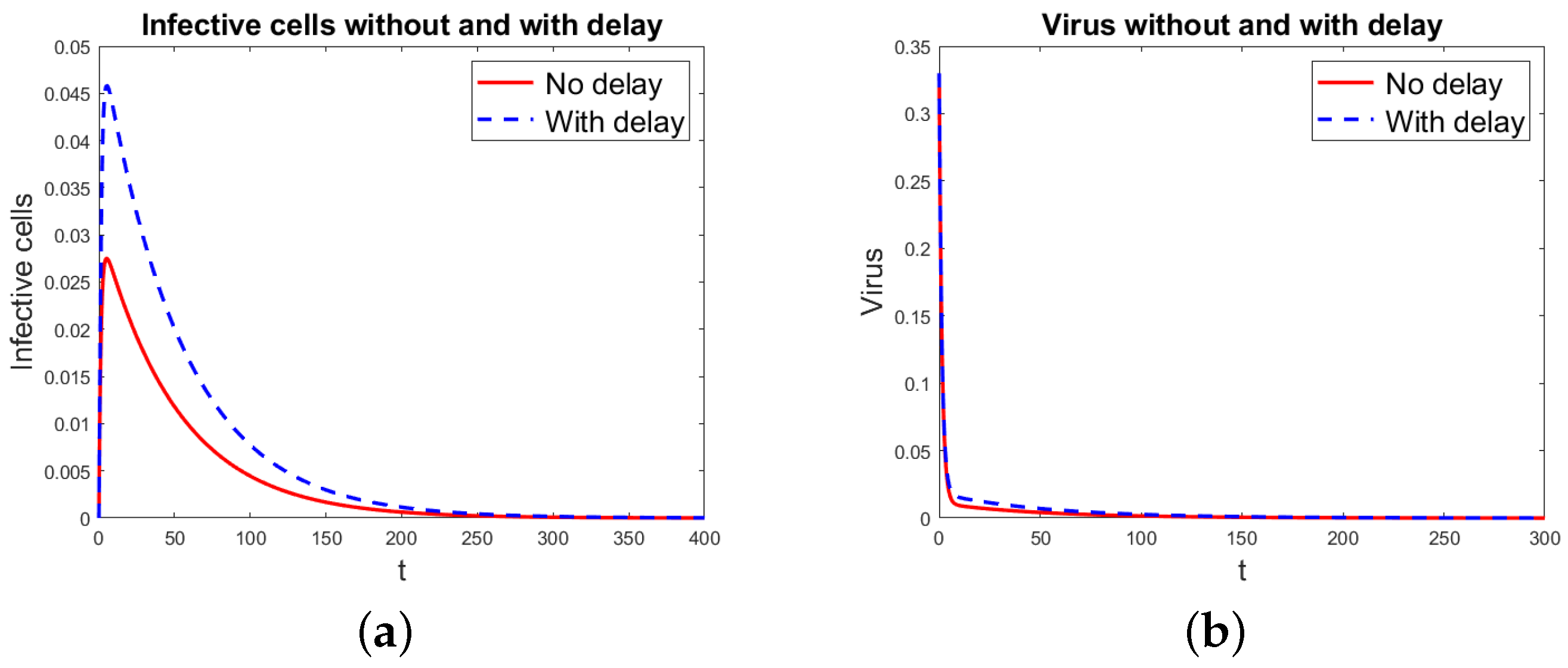
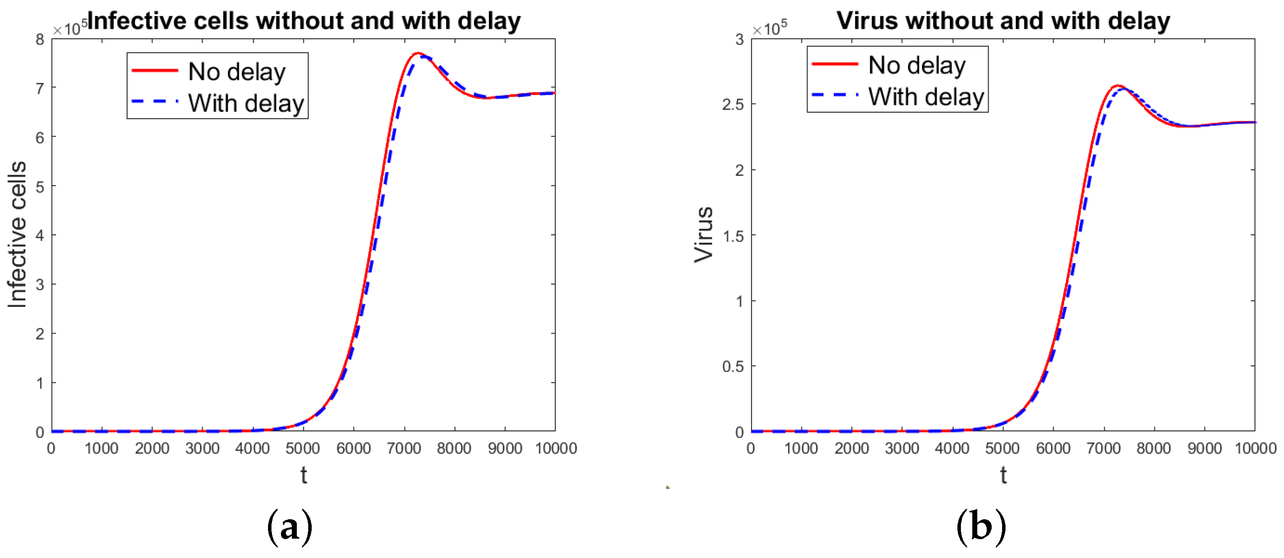
Figure 1 shows the simulation results for the basic virus propagation models (1) and (3), for infected cells and virus particles using the data in Table 1. The basic reproduction rate is $R_0$ = 0.5314, so the infection disappears with time. Figure 2 shows the results for the basic virus propagation models (1) and (3), for infected cells and virus particles with the data in Table 1, but with $\beta =8\times {10}^{-10}$. Now, $R_0=1.0629$, and the virus infection is chronic. Since the threshold index is very close to 1, it takes a long time for the infection to reach the chronic state, the time shown for the simulation is long, and the differences in the solution for the models without and with delay appear smaller than they are.

As expected for the basic models, (1) and (3), the simulated solutions look similar, with the delayed model’s infected compartments approaching the DFE more slowly than the model with no delay, for $R_0<1$. For $R_0>1$, the delayed model’s infected compartments increase faster. Since the corresponding threshold indices for both models are equal, for the given values of the parameters, both models make the same prediction about the persistence of the infection.

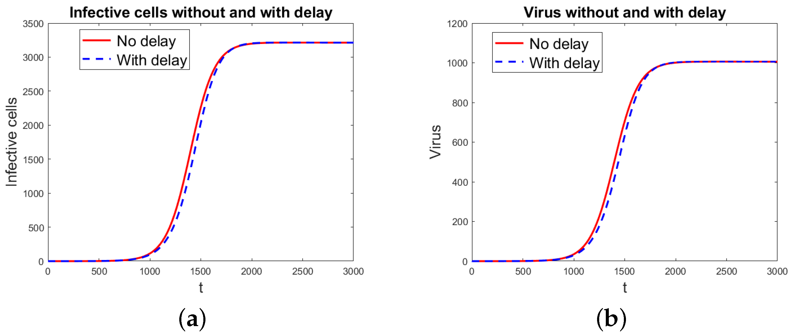
Figure 3 shows the simulation results using the virus propagation model 2 both without and with the two delays. The graphs are for infected cells and virus particles for the data in Table 1 and Table 2. For the model without delay, the threshold index using the next-generation matrix method is $R_{0NG}=1.0869$. For both the non-delayed and delayed models, the index using the characteristic equation is $R_{0CE}=1.1537$. So, both models predict an established infection. Since the threshold index is very close to 1, it takes a long time for the infection to reach the chronic state, the time of simulation shown is long, and the differences in the solution for the models without and with the two delays appear smaller than they are.

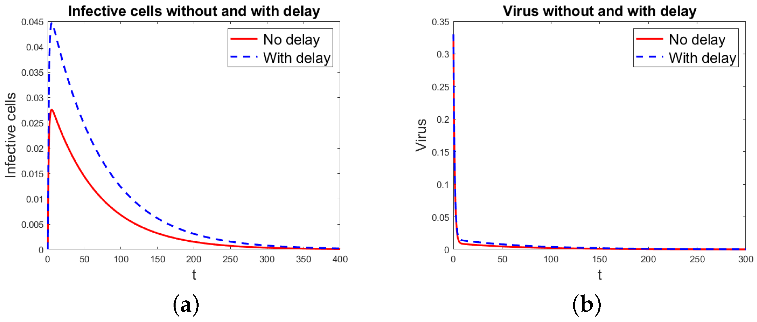
Figure 4 shows the simulation results using the virus propagation model 2 both without and with delay. The removal rate of infected cells by effector cells was changed to ${\beta }_{ey}=1$×${10}^{-3}$, and ${\beta }_{ve}={\beta }_{ev}$ was kept. The graphs are for infected cells and virus particles for the data in Table 1 and Table 2. For the model without delay, the threshold index using the next-generation matrix method is $R_{0NG}$ = 0.8780. For both the non-delayed and delayed models, the index using the characteristic equation is $R_{0CE}$ = 0.8952. So, both models predict the disappearance of the infection.

The comments made for the models (1) and (3) also apply to these two models, (2) and (5).

Simulations were also performed for the two scenarios using model 2 shown in Figure 3 and Figure 4, but assuming that the effector cells continue to be active after eliminating either an infected cell or a virus particle $({\beta }_{ye}={\beta }_{ve}=0)$. There were no significant changes in the plotted results.

In conclusion, there are several alternative threshold indices to the basic reproduction number. For models based on ODEs, the next-generation matrix method is a fairly simple way of obtaining one such index. For models based on DDEs, obtaining the index using the trascendental characteristic equation based on the diseased compartments works. Also, not all the parameters cause a significant change in the threshold indices.

4. Discussion

One of the most-important uses of mathematical models for virus propagation is to predict whether the infection is going to persist or not. For epidemic models, the basic reproduction number $R_0$, defined as the number of new infections due to one infected individual at the beginning of the infection, is often used for this purpose. For virus propagation within a host, it can be defined as the number of infected cells coming from one infected cell at the start of the process. For simple models as for the basic virus propagation model (1), it is easy to calculate from the definition, but not so for more-complicated models. For these models, an alternative index must be used. These indices are calculated from the analysis of the local asymptotic stability of the DFE or by determining whether the size of the infected compartments, that is infected cells and virus compartments, grows. These indices are usually chosen so that, when their value is greater than 1, the number of infected cells increases. The basic reproduction number also has this property. These other threshold indices, in general, do not predict the number of new infections, only whether the infections increase or not. But, whether the number of infected cells grows or not is the most-important information that the model can give. Many papers find a formula for the basic reproduction number or for an alternative index, but do not use it to predict whether the infection will persist or not. These papers usually do not mention how to reduce the value of the threshold index, so the infection dies or at least slows down. It may be trivial to reduce the value of some indices. For other indices, the partial derivatives of the index with respect to the parameters have to be taken and, even, a sensitivity analysis performed to determine the most-influential parameters. These papers instead perform numerical simulations. For some models, the threshold index calculated may be equal to $R_0$. But, this is not always the case. For models based on ODEs, the next-generation matrix method [40,41,42] is commonly used to determine a threshold index (usually called the basic reproduction number). It considers only the infected compartments at the beginning of the infection, and it is easy to calculate. For models like the model (1), the threshold index obtained by the next-generation matrix method is actually the square root of the basic reproduction number. For models based on DDEs, there is no new-generation matrix method. The methods used in this paper for the models (3) and (5) also consider only the compartments for infected cells and virus. The characteristic equation for the eigenvalues of the linearized about the DFE reduced system gives a condition for the DFE to be unstable, and a threshold index is obtained. Note that, for our delayed examples (3) and (5), the index obtained is the same as that for the corresponding non-delayed model. But, this is not always true. For example, the model given by (3) has an index that is different from the one from the model with no delay (1). Calculating a threshold index working only with the infected state variables and the corresponding characteristic equation to determine whether the DFE state is stable or not is usually a good strategy.

For most individuals, hepatitis B is not a chronic disease. When using the basic virus propagation model, the parameter more likely to significantly change from individual to individual is the cell infection rate $\beta$. So, based on this model, individuals with chronic hepatitis B have a lower $\beta$. In these cases, $\beta$ can be changed using antivirals. When considering the effect of the immune system, its action should be fundamental in whether the virus takes hold or not. The parameters ${\beta }_{ey}$ and ${\beta }_{ev}$ are fundamental in whether the threshold index is greater than 1 or not. In this paper, we just changed the value of ${\beta }_{ey}$ by less than a factor of two and the behavior changed. But, changes in ${\beta }_{ev}$ produce a similar effect. Individuals with immune deficiency and related disorders are known to be more likely to get chronic hepatitis B, and this probably causes a decrease in these rates. Also, newborns infected have about a 95% chance of developing chronic hepatitis B. The risk decreases with the age at the time of infection [2,52].

Another important use of mathematical models for hepatitis B is to determine the speed at which the infection grows or decays. The threshold indices previously calculated give an indication of this speed. The basic reproduction number tells the number of newly infected cells caused by one infected cell at the beginning of the infection. The other indices are not as accurate. For example, for the model given by (1), the index predicted by the new-generation matrix method is the square root of the basic reproduction number, so it predicts a slower growth when it is greater than 1. Numerical simulations predict the infection curves, but their accuracy depends on the validity of their hypotheses and on the data used to calibrate the model. The results found in this paper can also be used for other within-individual virus infection models such as those for influenza, HIV, or COVID-19 and even for epidemic models. On another note, vaccination is a commonly used strategy to reduce the spread of hepatitis B from individual to individual. A vaccinated individual will have a much stronger immune system. In a model that does not include the immune system, this can be performed by reducing the value of the infection rate parameter. If the immune system is taken into account, the parameters reflecting the effect of this system on the infected cells and virus particles can be adjusted. The result should be a threshold index very close to 0. The threshold indices are only useful for predicting the persistence or not of an infection when the parameters of the model are constant. In reality, the parameters may change with time since the immune system, replication of the virus, and other parameters may change. These changes may happen, for example, due to an illness or modifications of the life style of the individual.

Future work can include using more-complex mathematical models, for example adding active and latent effector cells, or innate and adaptive effector cells, or different types of effector cells. Treatment options, such as antiviral therapies, can also be included explicitly. Also, the effect of using additional latent cell populations instead of delays can be studied.

References

- Center for Disease Control and Prevention Web Page for Hepatitis B. Available online: https://www.cdc.gov/hepatitis/hbv/index.htm (accessed on 17 October 2023).
- World Heath Organization Web Page for Hepatitis B. Available online: https://www.who.int/news-room/fact-sheets/detail/hepatitis-b (accessed on 17 October 2023).
- Din, A.; Li, Y. Mathematical analysis of a new nonlinear stochastic hepatitis B epidemic model with vaccination effect and a case study. Eur. Phys. J. Plus 2022, 137, 1–24. [Google Scholar] [CrossRef]
- Wodajo, F.A.; Gebru, D.M.; Alemneh, H.T. Mathematical model analysis of effective intervention strategies on transmission dynamics of hepatitis B virus. Sci. Rep. 2023, 13, 8737. [Google Scholar] [CrossRef]
- Zada, I.; Naeem Jan, M.; Ali, N.; Alrowail, D.; Sooppy Nisar, K.; Zaman, G. Mathematical analysis of hepatitis B epidemic model with optimal control. Adv. Differ. Equ. 2021, 2021, 1–29. [Google Scholar] [CrossRef]
- Oludoun, O.; Adebimpe, O.; Ndako, J.; Adeniyi, M.; Abiodun, O.; Gbadamosi, B. The impact of testing and treatment on the dynamics of Hepatitis B virus. F1000Research 2021, 10, 936. [Google Scholar] [CrossRef]
- Anderson, R.M.; May, R.M. Infectious Diseases of Humans: Dynamics and Control; Oxford University Press: Oxford, UK, 1991. [Google Scholar]
- Nowak, M.A.; Bangham, C.R. Population dynamics of immune responses to persistent viruses. Science 1996, 272, 74–79. [Google Scholar] [CrossRef]
- Bonhoeffer, S.; May, R.M.; Shaw, G.M.; Nowak, M.A. Virus dynamics and drug therapy. Proc. Natl. Acad. Sci. USA 1997, 94, 6971–6976. [Google Scholar] [CrossRef] [PubMed]
- Nowak, M.; May, R.M. Virus Dynamics: Mathematical Principles of Immunology and Virology: Mathematical Principles of Immunology and Virology; Oxford University Press: Oxford, UK, 2000. [Google Scholar]
- Regoes, R.R.; Wodarz, D.; Nowak, M.A. Virus dynamics: The effect of target cell limitation and immune responses on virus evolution. J. Theor. Biol. 1998, 191, 451–462. [Google Scholar] [CrossRef] [PubMed]
- Pang, J.; Cui, J.A.; Hui, J. The importance of immune responses in a model of hepatitis B virus. Nonlinear Dyn. 2012, 67, 723–734. [Google Scholar] [CrossRef]
- Ciupe, S.M.; Ribeiro, R.M.; Perelson, A.S. Antibody responses during hepatitis B viral infection. PLoS Comput. Biol. 2014, 10, e1003730. [Google Scholar] [CrossRef]
- Wodarz, D.; Nowak, M.A. Mathematical models of HIV pathogenesis and treatment. BioEssays 2002, 24, 1178–1187. [Google Scholar] [CrossRef]
- Nowak, M.A.; Bonhoeffer, S.; Hill, A.M.; Boehme, R.; Thomas, H.C.; McDade, H. Viral dynamics in hepatitis B virus infection. Proc. Natl. Acad. Sci. USA 1996, 93, 4398–4402. [Google Scholar] [CrossRef]
- Kuang, Y. Delay Differential Equations: With Applications in Population Dynamics; Academic Press: Cambridge, MA, USA, 1993. [Google Scholar]
- Erneux, T. Applied Delay Differential Equations; Springer Science & Business Media: Berlin/Heidelberg, Germany, 2009; Volume 3. [Google Scholar]
- Ruan, S. Delay differential equations in single species dynamics. In Delay Differential Equations and Applications; Springer: Berlin/Heidelberg, Germany, 2006; pp. 477–517. [Google Scholar]
- Ciupe, S.M.; Ribeiro, R.M.; Nelson, P.W.; Dusheiko, G.; Perelson, A.S. The role of cells refractory to productive infection in acute hepatitis B viral dynamics. Proc. Natl. Acad. Sci. USA 2007, 104, 5050–5055. [Google Scholar] [CrossRef]
- Kim, H.Y.; Kwon, H.D.; Jang, T.S.; Lim, J.; Lee, H.S. Mathematical modeling of triphasic viral dynamics in patients with HBeAg-positive chronic hepatitis B showing response to 24-week clevudine therapy. PLoS ONE 2012, 7, e50377. [Google Scholar] [CrossRef]
- Zhang, T.; Wang, J.; Li, Y.; Jiang, Z.; Han, X. Dynamics analysis of a delayed virus model with two different transmission methods and treatments. Adv. Differ. Equ. 2020, 2020, 1–17. [Google Scholar] [CrossRef] [PubMed]
- Dagasso, G.; Urban, J.; Kwiatkowska, M. Incorporating time delays in the mathematical modelling of the human immune response in viral infections. Procedia Comput. Sci. 2021, 185, 144–151. [Google Scholar] [CrossRef] [PubMed]
- Yosyingyong, P.; Viriyapong, R. Global dynamics of multiple delays within-host model for a hepatitis B virus infection of hepatocytes with immune response and drug therapy. Math. Biosci. Eng. 2023, 20, 7349–7386. [Google Scholar] [CrossRef] [PubMed]
- Rihan, F.A.; Alsakaji, H.J. Analysis of a stochastic HBV infection model with delayed immune response. Math. Biosci. Eng. 2021, 18, 5194–5220. [Google Scholar] [CrossRef] [PubMed]
- Li, D.M.; Chai, B.; Wang, Q. A model of hepatitis B virus with random interference infection rate. Math. Biosci. Eng. 2021, 18, 8257–8297. [Google Scholar] [CrossRef]
- Goyal, A.; Liao, L.E.; Perelson, A.S. Within-host mathematical models of hepatitis B virus infection: Past, present, and future. Curr. Opin. Syst. Biol. 2019, 18, 27–35. [Google Scholar] [CrossRef] [PubMed]
- Pourbashash, H.; Pilyugin, S.S.; De Leenheer, P.; McCluskey, C. Global analysis of within-host virus models with cell-to-cell viral transmission. Discret. Contin. Dyn. Syst. Ser. B 2014, 19, 3341–3357. [Google Scholar] [CrossRef]
- Elbaz, I.M.; El-Metwally, H.; Sohaly, M. Viral kinetics, stability and sensitivity analysis of the within-host COVID-19 model. Sci. Rep. 2023, 13, 11675. [Google Scholar] [CrossRef] [PubMed]
- Huang, G.; Liu, A.; Foryś, U. Global stability analysis of some nonlinear delay differential equations in population dynamics. J. Nonlinear Sci. 2016, 26, 27–41. [Google Scholar] [CrossRef]
- Lv, J.; Ma, W. Global asymptotic stability of a delay differential equation model for SARS-CoV-2 virus infection mediated by ACE2 receptor protein. Appl. Math. Lett. 2023, 142, 108631. [Google Scholar] [CrossRef] [PubMed]
- Orosz, G. Hopf bifurcation calculations in delayed systems. Period. Polytech. Mech. Eng. 2004, 48, 189–200. [Google Scholar]
- Jiang, X.; Chen, X.; Chi, M.; Chen, J. On Hopf bifurcation and control for a delay systems. Appl. Math. Comput. 2020, 370, 124906. [Google Scholar] [CrossRef]
- Engelborghs, K.; Luzyanina, T.; Roose, D. Numerical bifurcation analysis of delay differential equations using DDE-BIFTOOL. ACM Trans. Math. Softw. 2002, 28, 1–21. [Google Scholar] [CrossRef]
- Cui, Q.; Xu, C.; Ou, W.; Pang, Y.; Liu, Z.; Li, P.; Yao, L. Bifurcation Behavior and Hybrid Controller Design of a 2D Lotka–Volterra Commensal Symbiosis System Accompanying Delay. Mathematics 2023, 11, 4808. [Google Scholar] [CrossRef]
- Ou, W.; Xu, C.; Cui, Q.; Pang, Y.; Liu, Z.; Shen, J.; Baber, M.Z.; Farman, M.; Ahmad, S. Hopf bifurcation exploration and control technique in a predator-prey system incorporating delay. AIMS Math. 2024, 9, 1622–1651. [Google Scholar] [CrossRef]
- Tang, L.S.; Covert, E.; Wilson, E.; Kottilil, S. Chronic hepatitis B infection: A review. JAMA 2018, 319, 1802–1813. [Google Scholar] [CrossRef]
- Volinsky, I. Mathematical Model of Hepatitis B Virus Treatment with Support of Immune System. Mathematics 2022, 10, 2821. [Google Scholar] [CrossRef]
- Hu, J.; Liu, K. Complete and incomplete hepatitis B virus particles: Formation, function, and application. Viruses 2017, 9, 56. [Google Scholar] [CrossRef] [PubMed]
- Tu, T.; Zhang, H.; Urban, S. Hepatitis B Virus DNA Integration: In Vitro Models for Investigating Viral Pathogenesis and Persistence. Viruses 2021, 13, 180. [Google Scholar] [CrossRef] [PubMed]
- Van den Driessche, P.; Watmough, J. Reproduction numbers and sub-threshold endemic equilibria for compartmental models of disease transmission. Math. Biosci. 2002, 180, 29–48. [Google Scholar] [CrossRef] [PubMed]
- Van den Driessche, P. Reproduction numbers of infectious disease models. Infect. Dis. Model. 2017, 2, 288–303. [Google Scholar] [CrossRef] [PubMed]
- Diekmann, O.; Heesterbeek, J.; Roberts, M.G. The construction of next-generation matrices for compartmental epidemic models. J. R. Soc. Interface 2010, 7, 873–885. [Google Scholar] [CrossRef] [PubMed]
- Hefferman, J.; Smith, R.; Wahl, L. Perspectives on the basic reproduction ratio. J. R. Soc. Interface 2005, 2, 281–293. [Google Scholar] [CrossRef] [PubMed]
- Murray, J.D. Mathematical Biology I. An Introduction; Springer: Berlin/Heidelberg, Germany, 2002. [Google Scholar]
- Allen, L. An Introduction to Mathematical Biology; Pearson-Prentice Hall: Old Bridge, NJ, USA, 2007. [Google Scholar]
- Wei, H.M.; Li, X.Z.; Martcheva, M. An epidemic model of a vector-borne disease with direct transmission and time delay. J. Math. Anal. Appl. 2008, 342, 895–908. [Google Scholar] [CrossRef]
- Al Basir, F.; Takeuchi, Y.; Ray, S.A. Dynamics of a delayed plant disease model with Beddington-DeAngelis disease transmission. Math. Biosci. Eng. 2021, 18, 583–599. [Google Scholar] [CrossRef]
- Wodarz, D. Mathematical models of immune effector responses to viral infections: Virus control versus the development of pathology. J. Comput. Appl. Math. 2005, 184, 301–319. [Google Scholar] [CrossRef]
- Zhang, S.; Li, F.; Xu, X. Dynamics and control strategy for a delayed viral infection model. J. Biol. Dyn. 2022, 16, 44–63. [Google Scholar] [CrossRef]
- Bauer, T.; Sprinzl, M.; Protzer, U. Immune control of hepatitis B virus. Dig. Dis. 2011, 29, 423–433. [Google Scholar] [CrossRef] [PubMed]
- Smith, H.L. An Introduction to Delay Differential Equations with Applications to the Life Sciences; Springer: New York, NY, USA, 2011; Volume 57. [Google Scholar]
- Lok, A.S.; McMahon, B.J. Chronic hepatitis B. Hepatology 2007, 45, 507–539. [Google Scholar] [CrossRef] [PubMed]
Figure 1.
Basic virus propagation model without and with delay. Notice that the number of virus particles is one order of magnitude larger than the number of infected cells, since each infected cell produces many virus particles. (a) Infected cells. (b) Virus particles.
Figure 2.
Basic virus propagation model without and with delay, but = 8 ×. (a) Infected cells. (b) Virus particles.
Figure 3.
Virus propagation model 2 without and with delay. (a) Infected cells. (b) Virus particles.
Figure 4.
Virus propagation model 2 without and with delay, but with = 1 ×. Notice that the number of virus particles is one order of magnitude larger than the number of infected cells, since each infected cell produces many virus particles. (a) Infected cells. (b) Virus particles.