Article

Modelling Microstructure in Casting of Steel via CALPHAD-Based ICME Approach

1
Swerim AB, SE-164 40 Kista, Sweden
2
Alleima AB, SE-811 81 Sandviken, Sweden
3
Uddeholms AB, SE-683 85 Hagfors, Sweden
*
Author to whom correspondence should be addressed.
Submission received: 27 October 2023 / Revised: 20 November 2023 / Accepted: 21 November 2023 / Published: 28 November 2023
(This article belongs to the Collection Feature Paper Collection of Advanced Research on Alloys)

Abstract

:
Integrated computational materials engineering (ICME) is emerging as an increasingly powerful approach to integrate computational materials science tools into a holistic system and address the multiscale modeling challenges in the processing of advanced steels. This work aims at incorporating macroscopic model (finite element-based thermal model) and microscopic model (CALPHAD-based microstructure model), building an industry-oriented computational tool (MICAST) for casting of steels. Two case studies were performed for solidification simulations of tool steel and stainless steel by using the CALPHAD approach (Thermo-Calc package and CALPHAD database). The predicted microsegregation results agree with the measured ones. In addition, two case studies were performed for continuous casting and ingot casting with selected steel grades, mold geometries and process conditions. The temperature distributions and histories in continuous casting and ingot casting process of steels were calculated using in-house finite-element code which is integrated in MICAST. The predicted temperature history from the casting process simulation was exported as input data for the DICTRA simulation of solidification. The resulting microsegregation by the DICTRA simulation can reflect the microstructure evolution in the real casting process. Current computational practice demonstrates that CALPHAD-based material models can be directly linked with casting process models to predict location-specific microstructures for smart material processing.

1. Introduction

Semi-finished products are mainly produced by continuous casting or by ingot casting. The casting process involves many physical phenomena including heat transfer, solidification, fluid flow, segregation, solid phase transformation, microstructure formation, hot crack and mechanical behavior [1,2,3,4]. Microstructure and possible defects during the solidification and cooling of steels are significant factors for the control of the properties and the quality of casting products. However, it is still very difficult to find a comprehensive fundamental approach to trace the microstructure evolution and defect formation along a given industrial process path. This is mainly due to solidification and microstructure occurring in a wide range of length scales (from the atomic scale to the dimension of the macroscopic process) and non-equilibrium states in real casting processes. Multiscale modeling and its supporting numerical computation methods are playing an increasing role in understanding and interpreting experimental observations and reducing experimental costs associated with microstructural evolution [5,6,7,8].
Numerical simulation of casting processes has been quite mature at the macroscopic level [9,10,11,12,13], including the finite difference method (FDM), finite element method (FEM) and finite volume method (FVM). Based on these methods, commercial simulation software [14] for the casting process have been developed, such as ProCast, Thercast, MAGMASoft, and Flow3D. These simulation tools [15,16,17,18,19,20,21,22] allow prediction of temperature, fluid flow, distortion, stress and even microstructure in continuous casting or ingot casting. The main key issues are the properties and microstructural features of materials which play an important role in numerical simulations.
Phase and property diagrams are often used to understand the solidification path of steel. More generally, computational thermodynamics or the so-called CALPHAD (Calculation of Phase Diagrams) methods [23] are used for this purpose. Equilibrium (lever rule) and non-equilibrium (Scheil–Gulliver) models are two approximate models to predict the solidification path in a simple and efficient way without evoking complex kinetic calculations. Furthermore, a full diffusion model can result in an extension of the Scheil model by taking into consideration the back-diffusion in the solid. Microsegregation is an inevitable phenomenon in the solidification process, which occurs due to solute redistribution during solidification. It has an important influence on the subsequent metallurgical process and the final quality of the steel. It has also significant effects on macrosegregation, hot tearing formation, particle precipitation and phase transformation. Microsegregation in the solidification of steels has been the topic of many investigations [3,4,24,25,26,27,28,29,30]. A practical example of predicting microsegregation during solidification using a steel with composition 0.4 wt.%C-0.8 wt.%Mn-0.7 wt.%Si-0.03 wt.%P is given by Thermo-Calc [31].
Nowadays, integrated computational materials engineering (ICME) is emerging as a promising tool for developing advanced materials and improving manufacturing processes to meet challenging goals quickly and efficiently [32,33,34]. As a key component of the ICME approach, CALPHAD-based material properties and microstructures are utilized in the integrated numerical approach, making it possible to model the solidification with focus on microstructural evolution during the casting of steels. Incorporation of these software tools into a simultaneous manufacturing and product engineering process will result in improved computational efficiency and make correct information available at the right time. The application of ICME will accelerate materials development, design and manufacturing.
The slow transition of science-based materials calculation tools to engineering tools and the lack of materials engineers trained to use these tools have hindered ICME’s industrial acceptance in the casting of steels. This situation in Sweden has been improved via continuous development of the ICME-based computational tool—MICAST [35,36].
The present work describes the CALPHAD-based ICME approach employed in a MICAST platform for continuous casting and ingot casting of steels, which is being utilized by industrial users. The simulation results for the processes (continuous casting and ingot casting) and their microstructural evolutions are presented. It is emphasized that this work aims to predict microsegregation as a part of microstructure modeling in the ICME framework for steel casting.

2. Theory and Methods

2.1. Thermodynamic and Kinetic Calculation for Solidification

Computational thermodynamics and the so-called CALPHAD method are well established [37,38]. It can be used to predict phase equilibria and thermodynamic properties for complex multi-component systems, and can be extended to prediction of material properties, alloy design and processes optimization.
Different simplified models for simulating solidification of alloys are available. One of the most frequently used models is the Scheil–Gulliver model [39,40] (Figure 1). Scheil solidification assumes infinitely fast diffusion of all elements in the liquid and no diffusion in solid phases once they are formed. In this case, equilibrium exists at the solid–liquid interface and so compositions from the phase diagram are valid. In Thermo-Calc [41], this model is expanded by considering back-diffusion of interstitial elements (such as C and N in steels) in the solid phase. In the recent version of Thermo-Calc, Scheil with a simultaneous diffusion calculation in the primary phase is available, which requires additional kinetic data and takes dendrite spacing and cooling rate into account.
The equilibrium solidification and the Scheil–Gulliver models provide a fast and reliable method of determining the key phenomena and microstructural features during solidification.
An even more accurate approach would be necessary to consider diffusion of all elements both in the liquid and the solid phases during solidification. This is possible in DICTRA (The diffusion module as an add-on module to Thermo-Calc [41]), which is based on the numerical solution of the multi-component diffusion equations and the CALPHAD approach. DICTRA solves the liquid/solid phase transformation in one dimension, where local equilibrium is assumed to hold at the phase interface. It is meant that the chemical potentials of all elements are continuous across the boundary, but the chemical potential gradients are, in general, discontinuous. To maintain mass balance a set of flux balance equations must be satisfied at the phase interface [43]:
v α / γ ( c k α c k γ ) = J k α J k γ k   =   1 ,   ,   n     1
where v is the interfacial velocity. The concentrations (c) and the fluxes (J) are those at the interface and on the sides, respectively. Information regarding the size of the computational domain and the temperature as a function of time are to be determined before performing a DICTRA solidification simulation.
An example solidification process was simulated for AISI 314 steel (0.02 wt.%C, 2.7 wt.%Si, 1.75 wt.%Mn, 23.5 wt.%Cr, 19.4 wt.%Ni) stainless steel using two different methods as shown in Figure 2. The DICTRA calculation was set-up assuming a secondary dendrite arm spacing of ~200 μm (calculation domain of 100 μm) and constant cooling rate of 1 °C/s. Figure 2a shows the solidification path for AISI 314 stainless steel during peritectic solidification. The orange curve corresponds to the Scheil–Gulliver model (with carbon as fast diffuser), and the blue curve to a DICTRA simulation. It is seen that Scheil simulation results in an unrealistically low final solidification temperature compared to DICTRA simulation. Figure 2b shows Si, Mn, Cr and Ni enrichment in remaining liquid at the growth front during solidification as predicted by the Scheil–Gulliver model, demonstrating significant microsegregation. In terms of simulation time, the DICTRA calculation takes longer than the Scheil–Gulliver calculation.

2.2. Thermal Model

The thermal energy conservation equation for transient heat conduction is expressed as:
ρ C p T ˙ = ( k T ) + Q
k T = q h c ( T T a ) ε σ ( T 4 T a 4 )
where T is the temperature, ρ is the density of material, Cp is the specific heat of material, k is the thermal conductivity of material, Q is the latent heat source, q is the input heat flux, hc is the heat transfer coefficient under natural convection, σ is the Stefan–Boltzmann constant, Ta is the ambient temperature, and ε is the emissivity.
The explicit model used here solves the standard heat conduction equation using the finite element method for spatial integration and marches through time using the fully explicit “forward finite-difference” method:
T i + 1 = T i + Δ t i + 1 T ˙ i
The temperature is computed directly without any iteration:
T ˙ i = C 1 ( P i F i )
where C is the lumped thermal capacity matrix, P is the applied source vector, F is the internal thermal flux vector,  T ˙    is the changing rate of temperature.
The thermal stable time increment is generally defined by the condition that, within the time increment, the thermal wave must not propagate a distance longer than the minimal dimension of any finite element in the mesh. Consequently, the thermal stable time increment is defined as
Δ t min ( L e 2 ) 2 α
where Le is the smallest element edge length, while α is the thermal diffusivity of material.
Obtaining a unique solution to the heat transfer equation involves declaring the boundary conditions of the heat transfer problem.
For a two-dimensional problem the transient temperature field on the cross-section of cast strand for each time step is computed by using Equations (4) and (5) as well as boundary conditions based on Equation (2).
For continuous casting of billets, the Lagrangian approach of a cross-section slice through the strand is employed, ignoring the axial heat conduction. A three-dimensional temperature field is obtained by moving the cross-section from entry to exit of the control volume. The strand core eventually becomes fully solidified when it reaches the “metallurgical length”.
For ingot casting, only solidification processes for the specified vertical 2D cross-section are analyzed. A series of temperature fields for all parts (metal, mold, riser insulator, powder) are resulting for a specified cooling time.

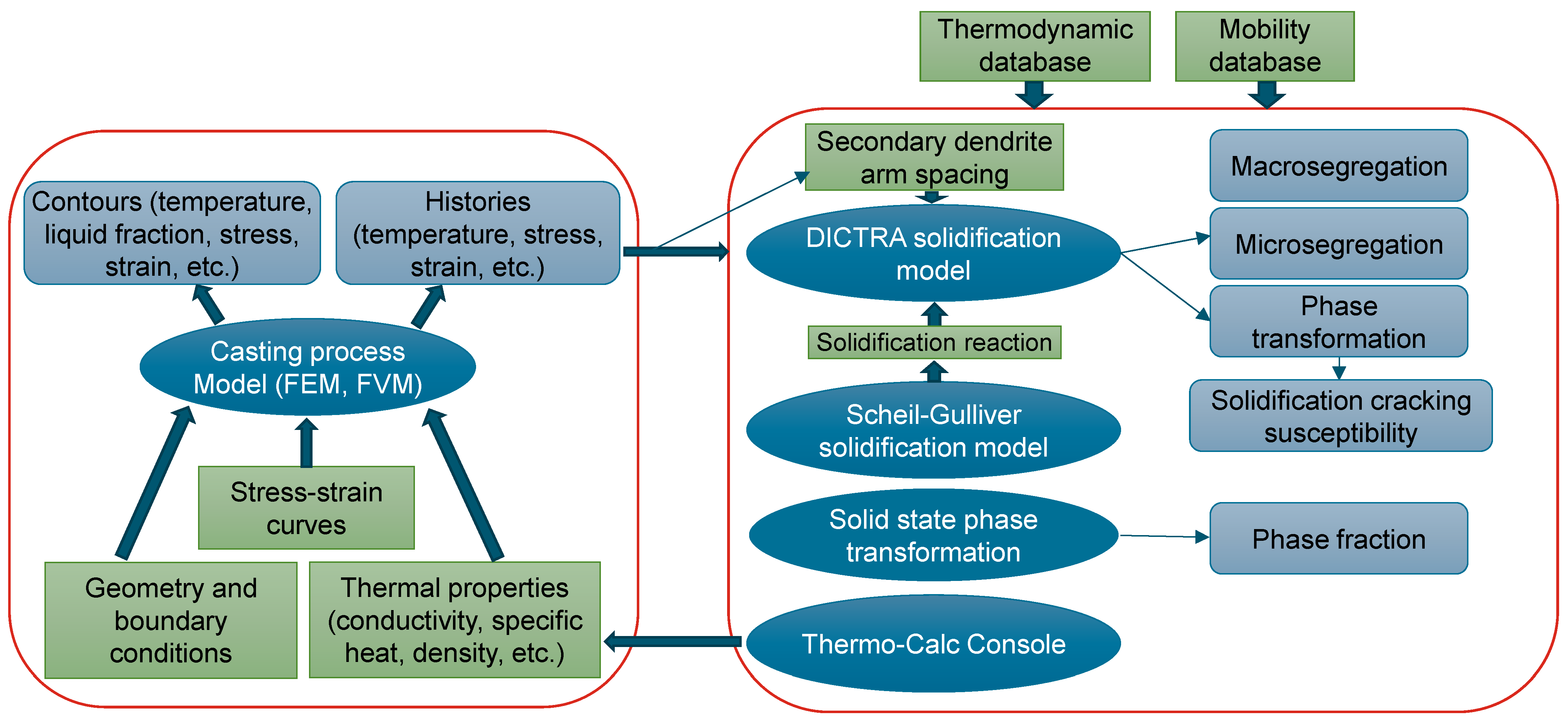
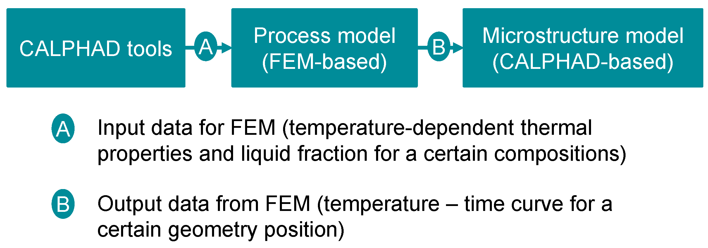
2.3. Model Integration

The link between macroscopic casting process simulations and CALPHAD solidification models allows simplification of the complex process–microstructure relationship in the casting of steels based on the effect of processing and compositions on temperature history at the microstructural scale. Figure 3 shows a schematic diagram for the CALPHAD-based ICME approach on a MICAST platform. It demonstrates how CALPHAD tools and FEM can be linked together in ICME frameworks. At first, temperature and chemistry-dependent thermophysical properties are obtained via CALPHAD tools (Thermo-Calc [41], IDS [44]) as input data for FEM, giving more accurate predictions. Secondly, the predicted temperature information is applied as input data for DICTRA simulation for getting detailed microsegregation and phase transformation prediction. This approach is summarized in Figure 4, which was used for the present work. In actual calculations, Scheil calculations are first performed to obtain preliminary information about possible solidification paths and microsegregation profiles before performing real DICTRA calculations.
Currently, only a heat transfer thermal model for the casting process is integrated into the MICAST platform. More advanced models (for example, FEM-based stress and strain analysis, and FVM-based flow and thermal analyses) for specified industrial casting processes are being integrated into the MICAST computational platform. It is also expected that the computational tools will have no limitation on the complexity of alloys through coupling with CALPHAD databases, which is the benefit of the ICME approach.
MICAST is designed as a workspace, which may include multiple modules for performing a variety of simulations and can be easily extended. Currently, two modules are available, which are the Property and Microstructure module for multi-component thermodynamic and kinetic calculations, and the Process simulation module for casting process simulation, including continuous casting and ingot casting.
This ICME framework can be achieved by incorporating macroscopic models (finite element-based thermal models) and microscopic models (CALPHAD-based microstructural models), building an industry-oriented computational tool (MICAST) for casting of steels. MICAST can deliver a user-friendly interface which allows industrial users to get started quickly. All Thermo-Calc and DICTRA calculations as well FEM calculations can be performed within the MICAST interface without any coding. The integrated commercial Thermo-Calc extensive database allows modeling of any steel grades or alloys covered by these databases.
In the present work, DICTRA simulations were performed with input thermodynamic, mobility, and kinetic-parameter databases as well as solidification conditions (alloy composition, cooling rate or temperature–time curve) to predict solidified phases and their fractions, SDAS (secondary dendrite arm spacing), and distribution of solutes with each phase. Those predicted results form the basis of subsequent microstructural analyses.

3. Results and Discussions

For all selected alloys, Thermo-Calc and DICTRA were used first to carry out equilibrium calculation, Scheil calculation and DICTRA calculation inside the MICAST interface, focusing on solidification simulation of steels. This is described in Section 3.1.
Then the process simulations for both continuous casting and ingot casting were performed by MICAST process simulation modules together with pre-calculated material thermal properties by CALPHAD tools. Furthermore, DICTRA simulations were performed to predict microsegregation using temperature history data from FEM. This is described in Section 3.2.

3.1. General Solidification

A solidification calculation for austenitic stainless steel 904L (Fe-0.01 wt.%C-0.35 wt.%Si-1.7 wt.%Mn-20 wt.%Cr-25 wt.%Ni-4.3 wt.%Mo-1.5 wt.%Cu) was performed using DICTRA, assuming secondary dendrite arm spacing of 56 µm (estimated from the measurement of concentration profiles), constant cooling rate of 1.0 °C/s, starting temperature of 1438 °C. Samples taken from continuously cast 150 × 150 mm billet of stainless steel were used for EPMA studies, which were prepared by grinding and polishing. EPMA measurements were performed on cross-sectional samples without etching for studying the microsegregation of an as-cast structure using a Jeol JXA 8530F Plus Hyperprobe, equipped with a field emission gun with five spectrometers plus an additional EDS detector. The subsequent data-processing including quantification, and image processing was carried out.
Another solidification calculation for tool steel (Fe-0.39 wt.%C-1.0 wt.%Si-0.4 wt.%Mn-5.2 wt.%Cr-0.9 wt.%V) was performed using DICTRA, assuming secondary dendrite arm spacing of 12.6 µm (estimated from the measurement of concentration profiles), constant cooling rate of 180 °C/s, and starting temperature of 1500 °C. One piece of sample (~150 g) was taken from the steel product after heat treatment. The sample was put inside an alumina crucible and heated up in a lab-scale induction furnace with argon gas protection. When the steel was fully melted, it was poured into a copper mold and solidified under room temperature. After grinding and polishing, the specimen was etched to reveal solidification structures using Nital 5% etching reagent. This sample was observed using a scanning electron microscope (SEM-EDX) (FEI-QUANTA600FEG-D8366). The dendrite microstructure and composition distribution of elements were analyzed.
These experiments designed on one stainless steel and one tool steel aims at validating the calculated microsegregation of elements. A comparison function between experimental and calculated microsegregation has been integrated into the MICAST program.

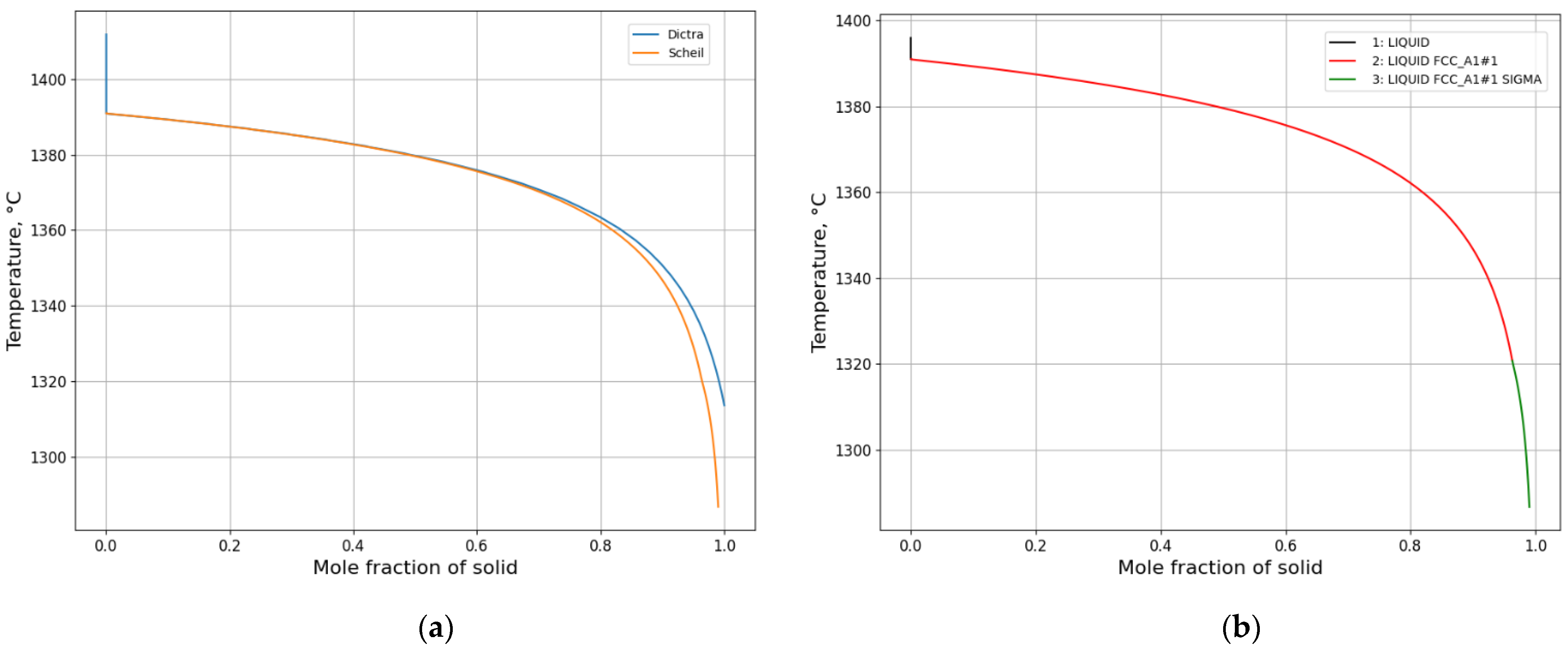
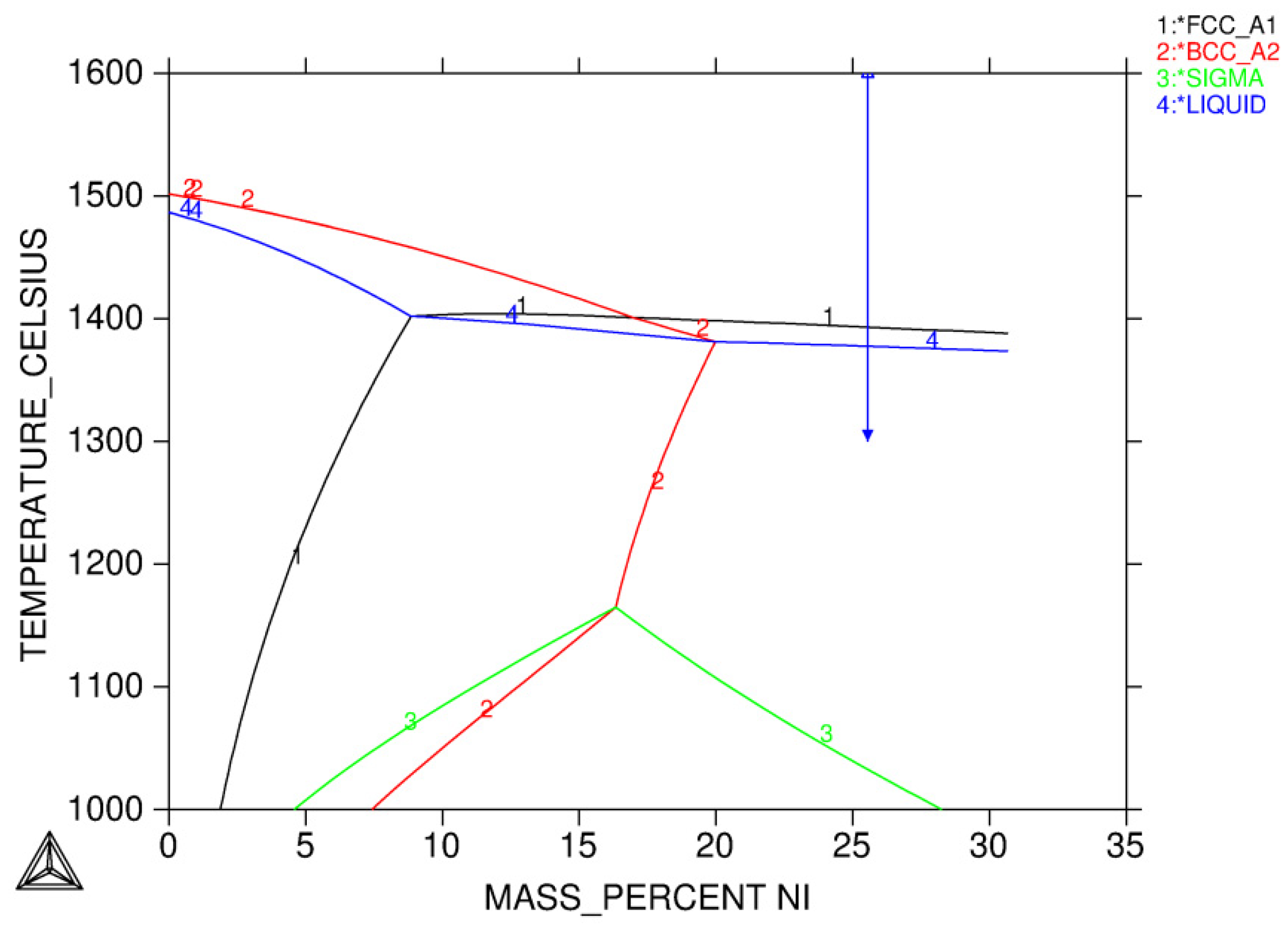
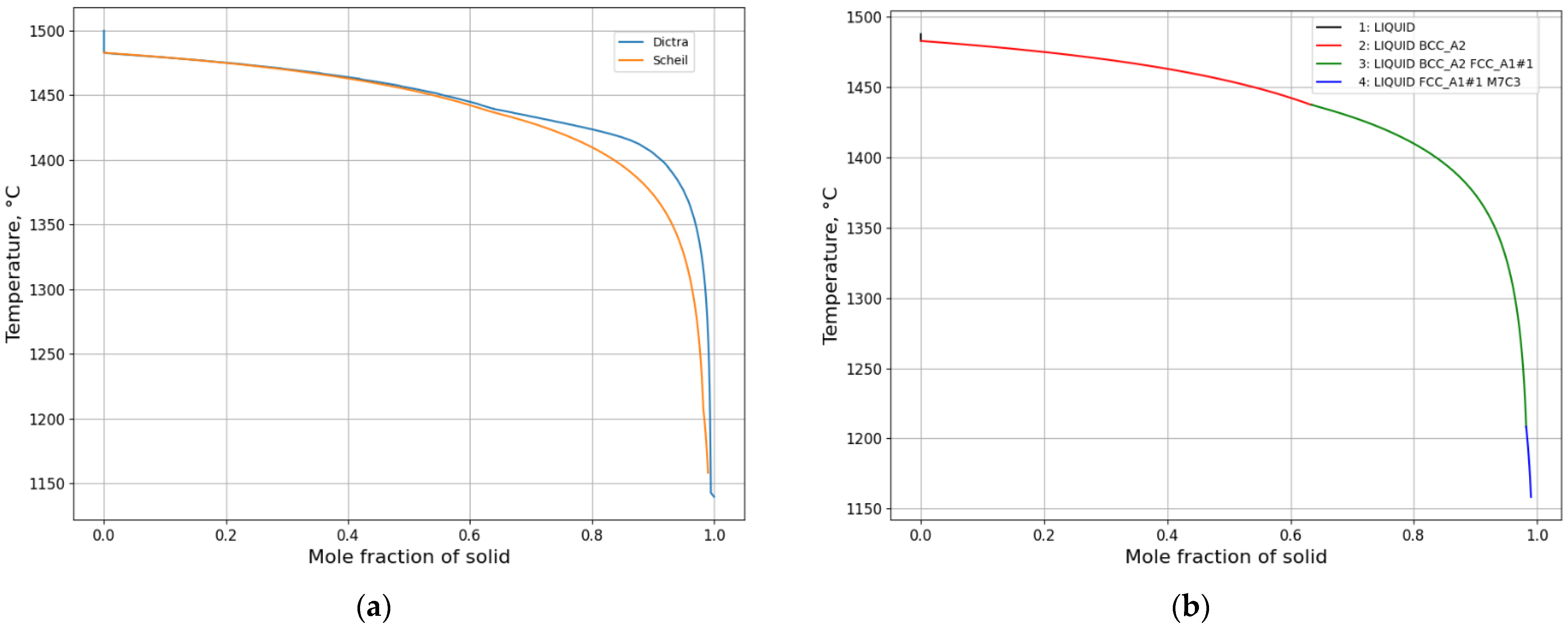
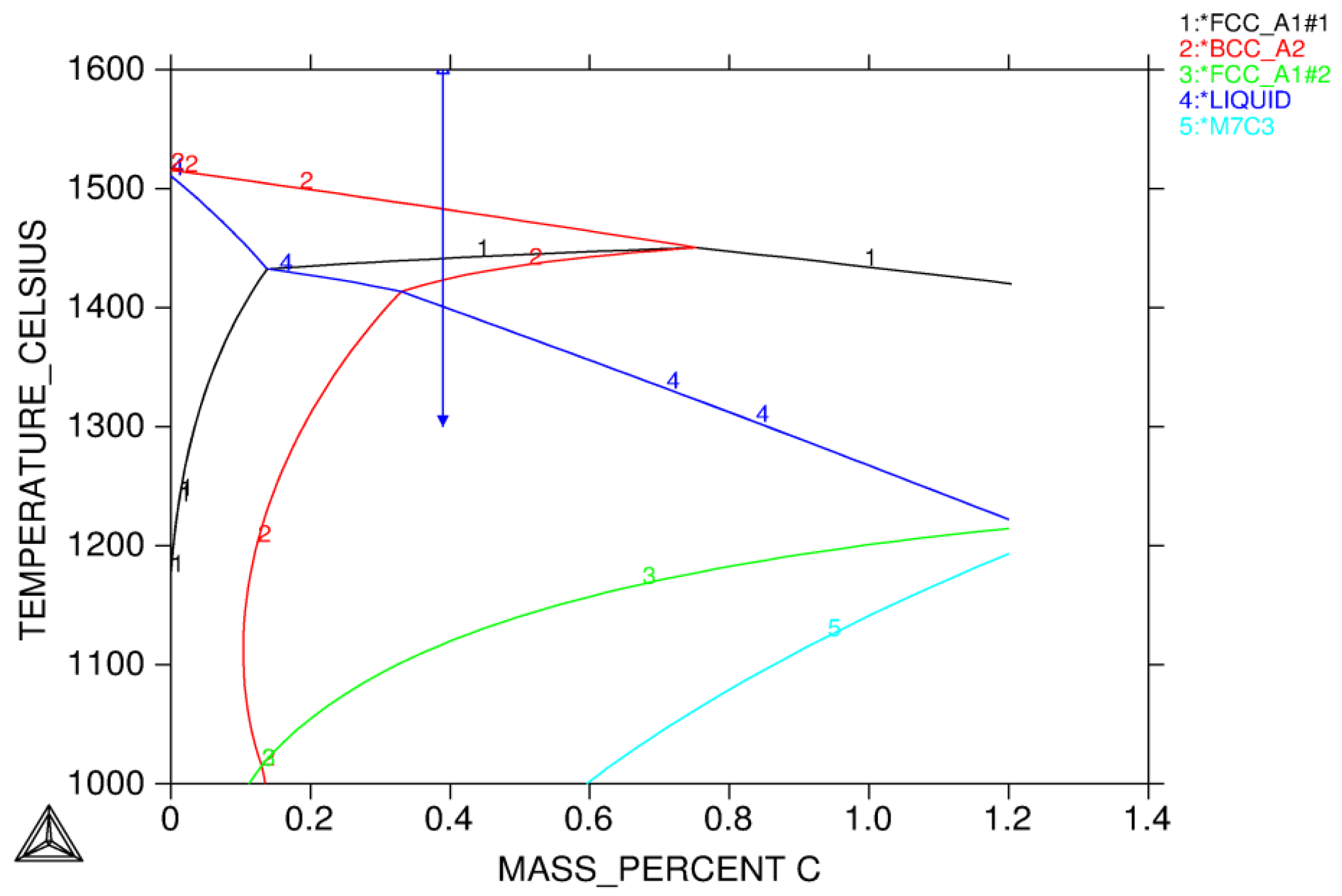
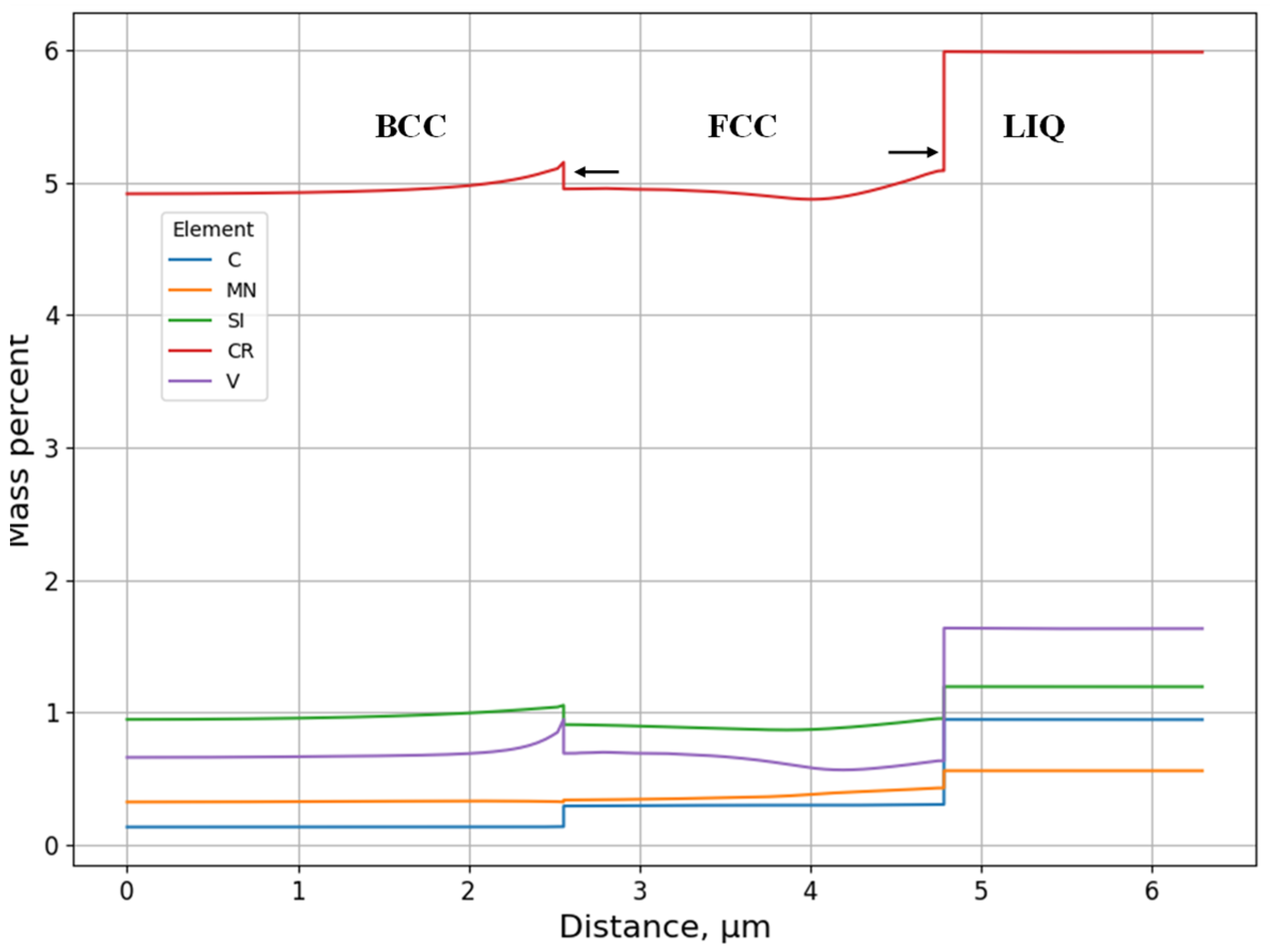
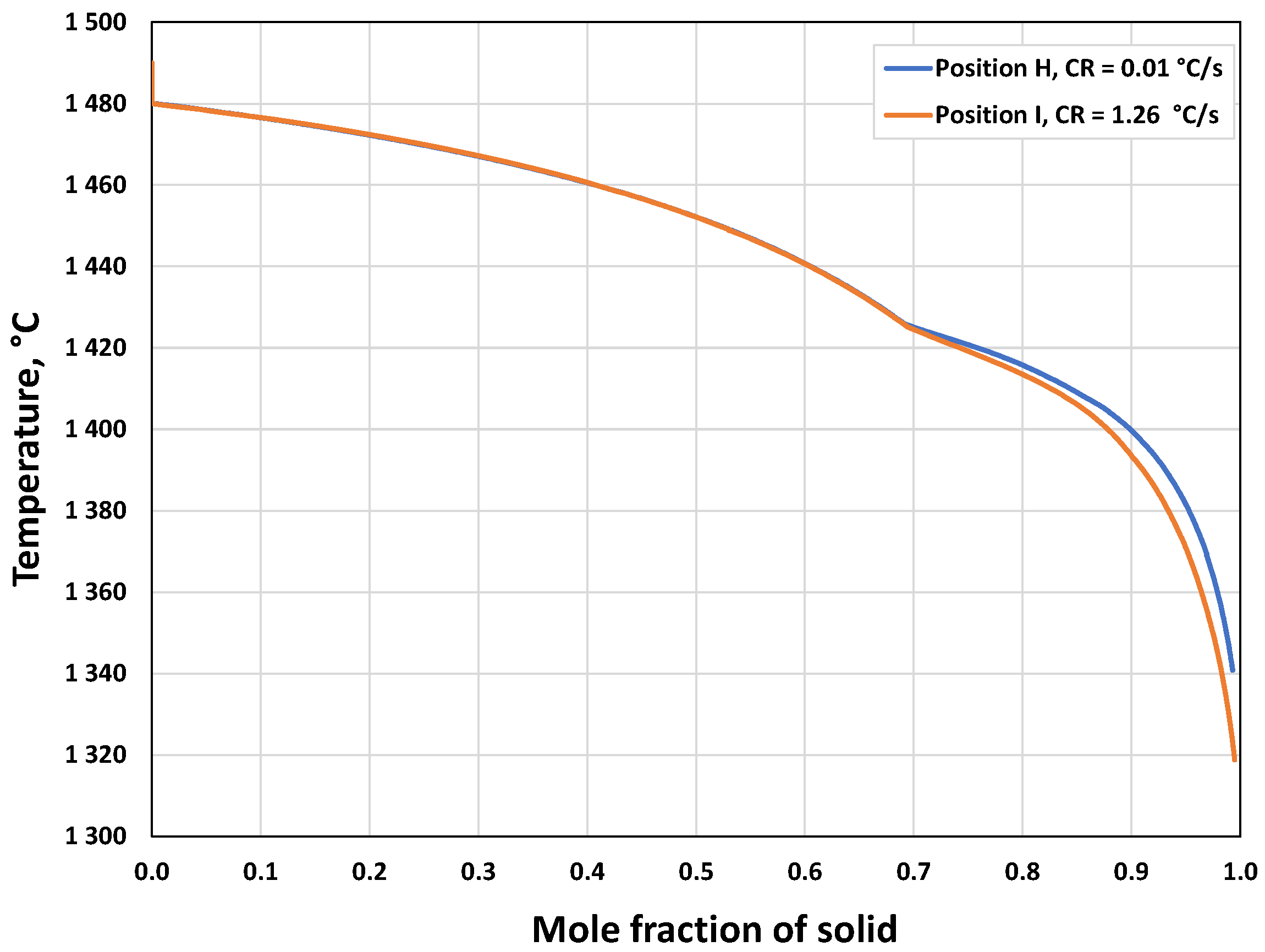
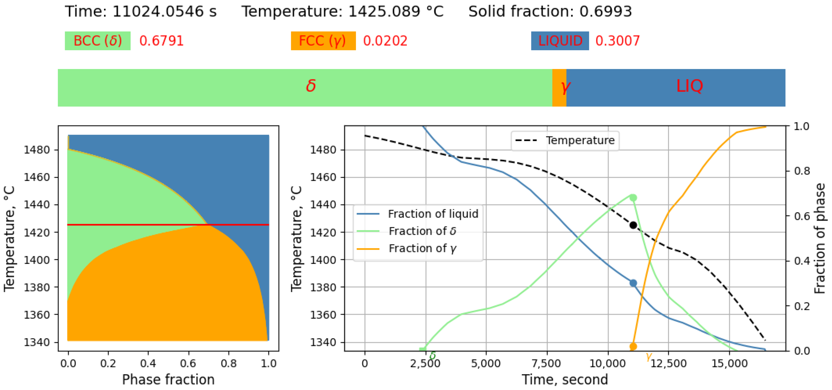
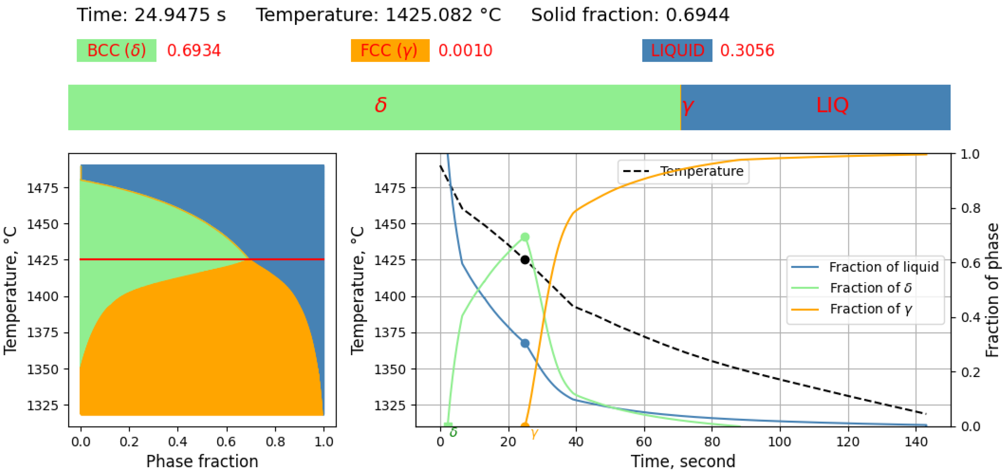
3.1.1. Solidification Path Diagram

Figure 5 shows the mole fraction of solid as a function of temperature from two solidification simulations of the specified stainless steel. It is seen from Figure 5a that the solidification follows the same path from the beginning and deviates from about 1370 °C, finishing with a higher solidus temperature when using DICTRA. The calculated solidus temperature 1314 °C by using DICTRA is closer to the measured value (1328 °C). It is shown from Figure 5b that liquid is transformed directly to austenite at the first stage and then the sigma phase appears during solidification from the Scheil calculation. It should be pointed out that the sigma phase is not set as product phase to be formed in the DICTRA simulation.
A stable Fe–Ni isopleth phase diagram is shown in Figure 6. A vertical line with an arrow is drawn to indicate the possible solidification path from liquid at the designed nickel content. The FCC phase is first formed. The solidification path according to Figure 5 and Figure 6 is expressed as:
LL + γ ⇒ L + γ + σ
where L is liquid phase, γ is austenite phase, σ is sigma phase.
Figure 7a shows a comparison for the calculated solid fractions between Scheil and DICTRA for the specified tool steel. It is seen that the solidification follows the same path from the beginning and deviates from about 1450 °C, finishing with higher solidus temperature when using DICTRA. The starting temperature is 1500 °C and simulation time is 2 s, giving an ending temperature 1140 °C. It is found from Figure 7b that liquid is transformed to δ ferrite at first stage and then the austenite phase appears during solidification from the Scheil calculation. No M7C3 phase is set as the phase formed in the DICTRA simulation.
A stable Fe–C isopleth phase diagram is shown in Figure 8. A vertical line with arrow is drawn to indicate the possible solidification path from liquid. BCC phase is first formed, FCC is decomposed from BCC and liquid.
The liquid is solidified through the peritectic reaction which means before liquid is fully transformed to δ-ferrite, austenite nucleates at the δ-ferrite/liquid interface as illustrated in Figure 7 and Figure 8. The solidification sequence is written as:
LL + δ ⇒ L + γ + δ ⇒ γ
where L is liquid phase, δ is ferrite phase, γ is austenite phase.

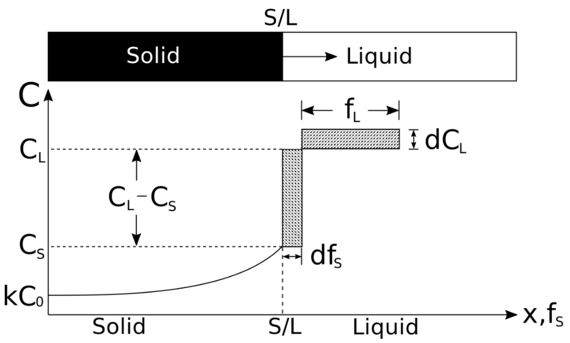
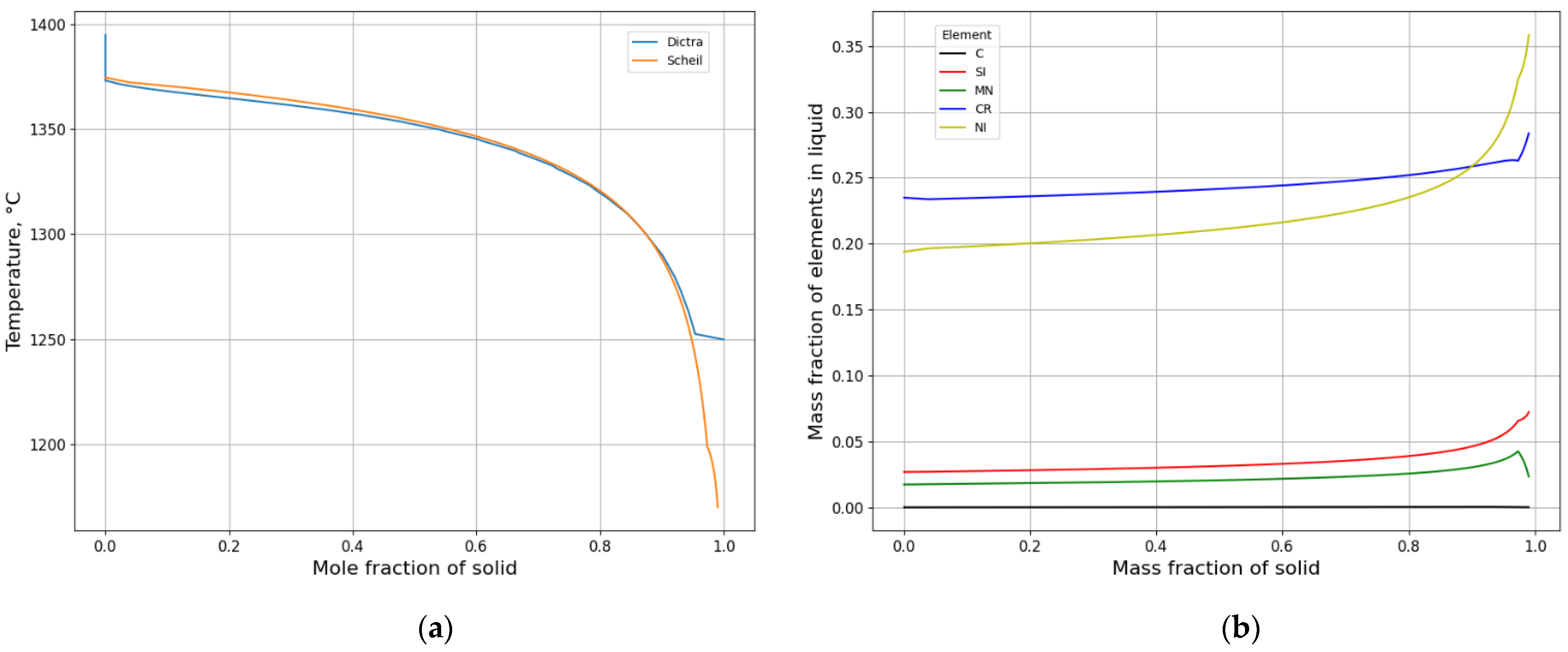
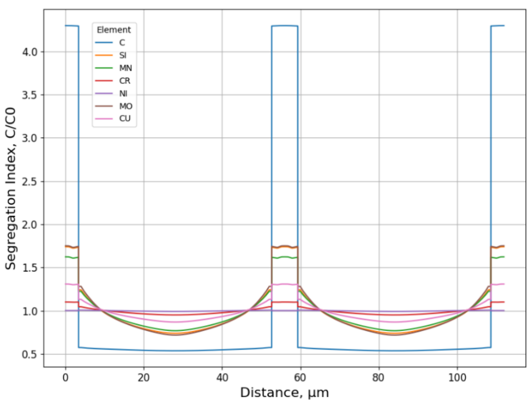
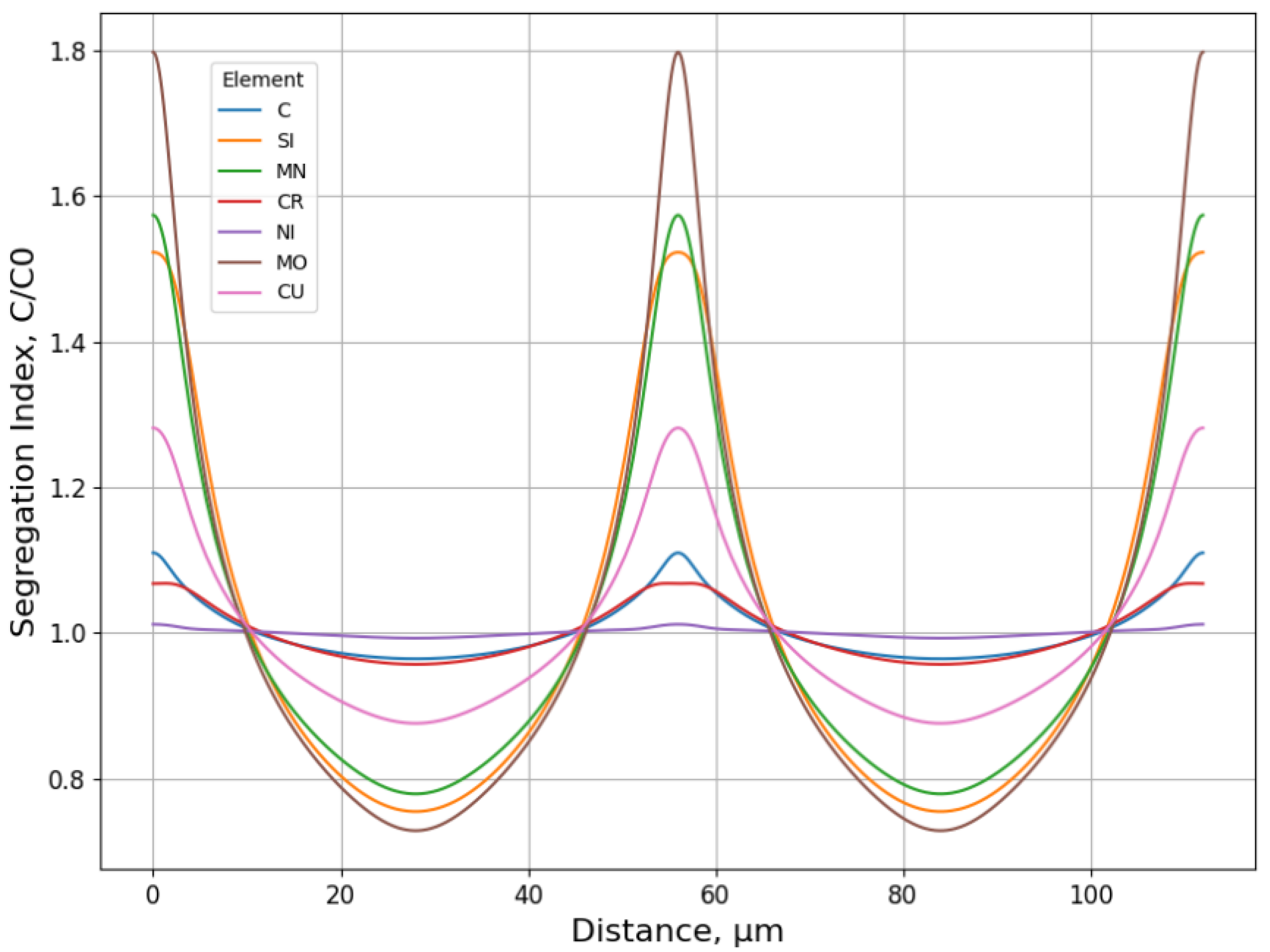
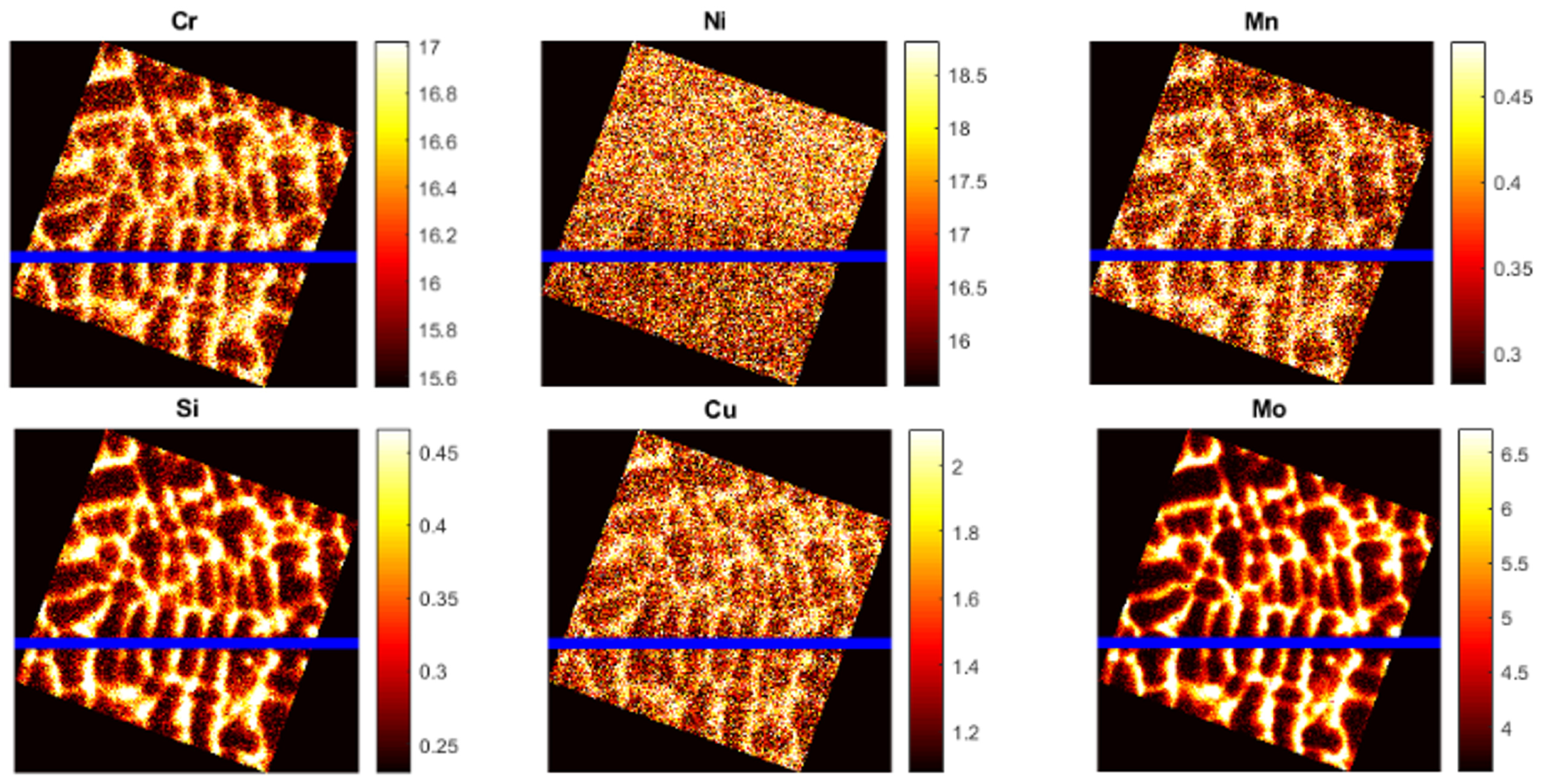
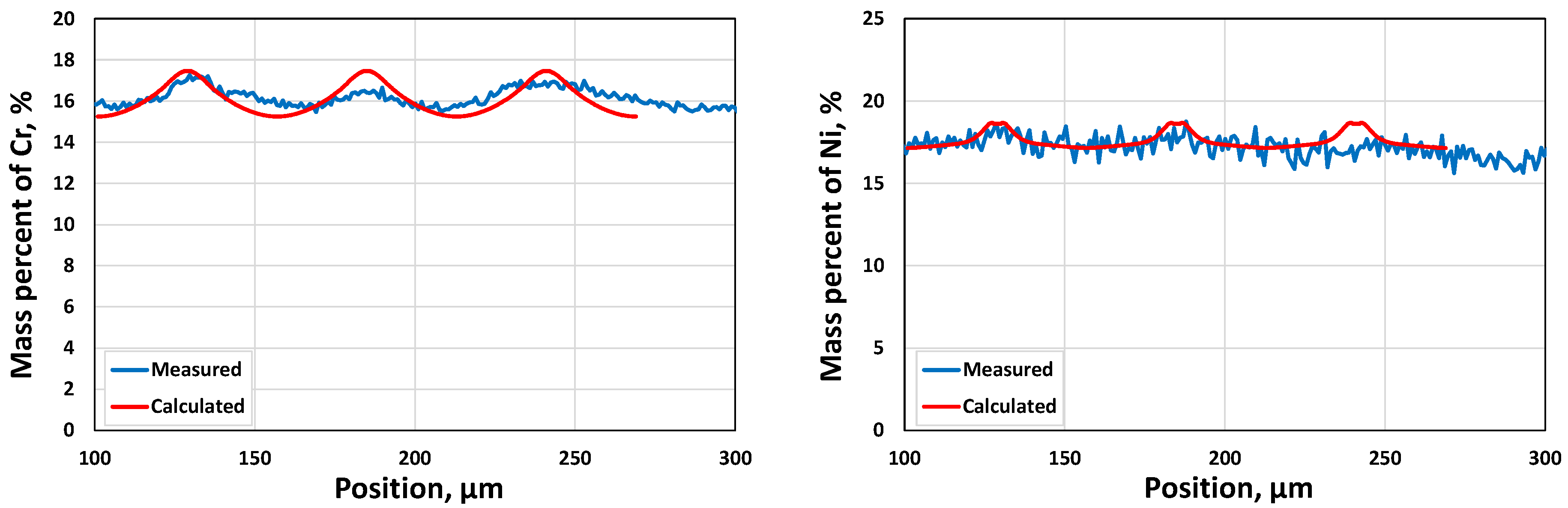
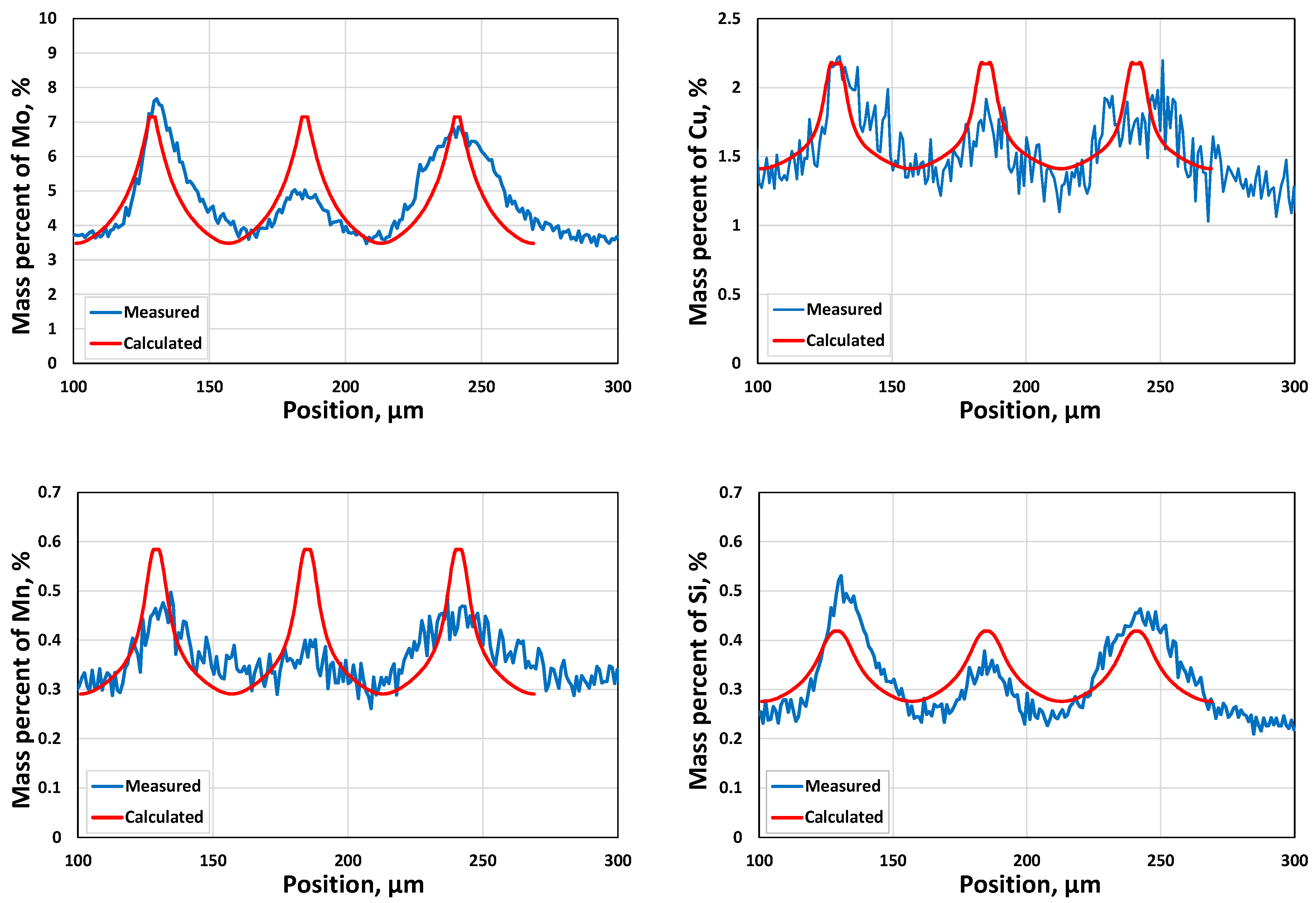
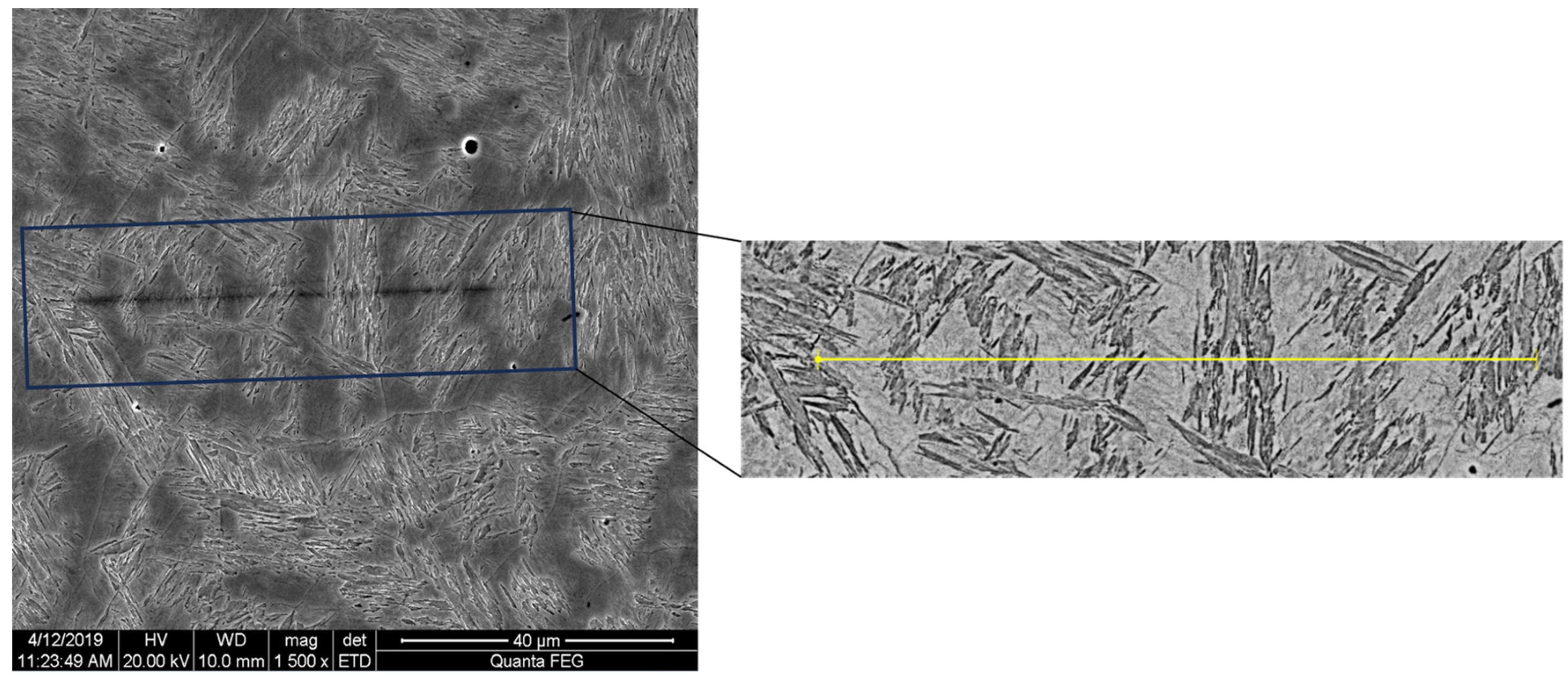
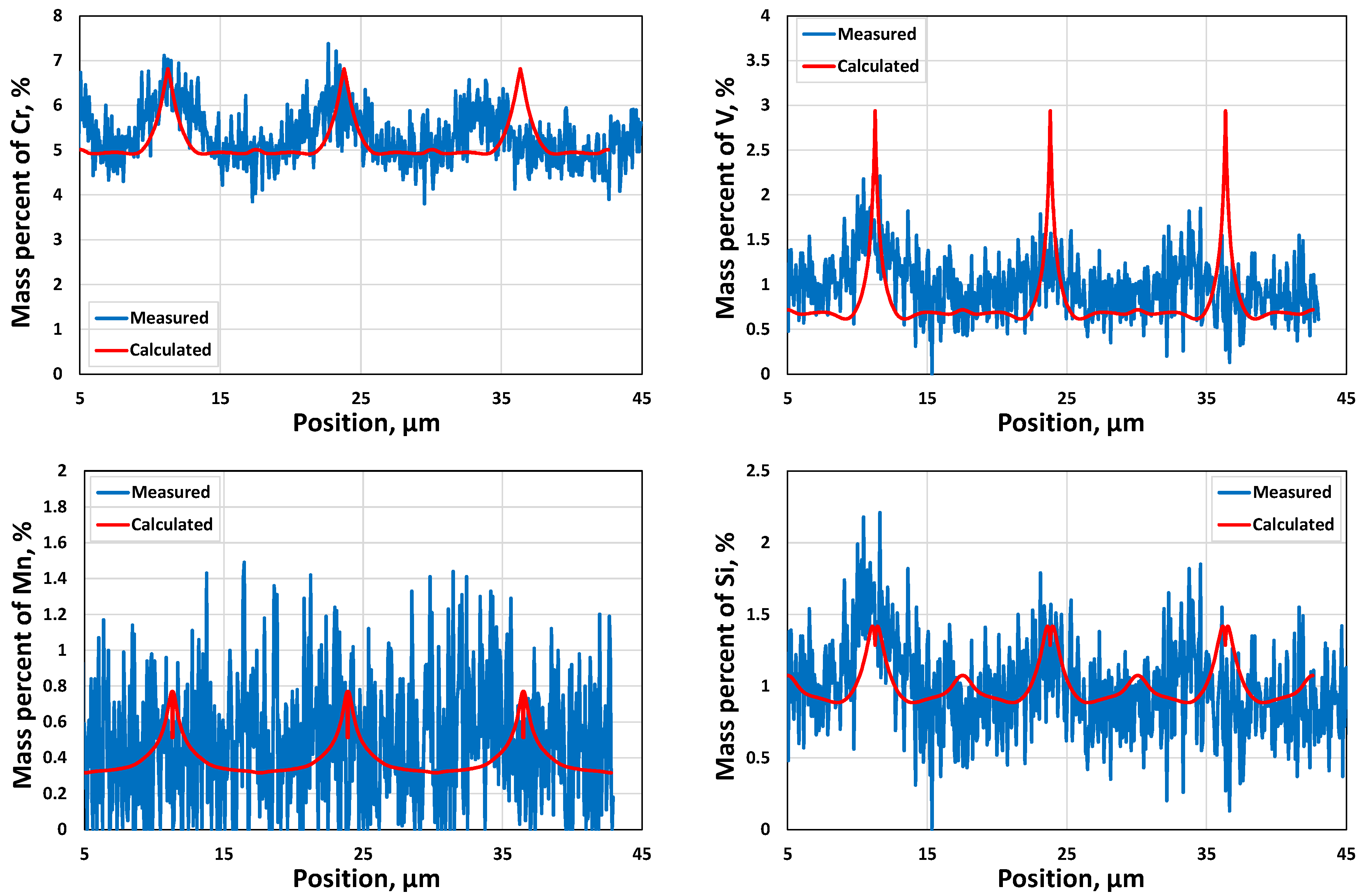
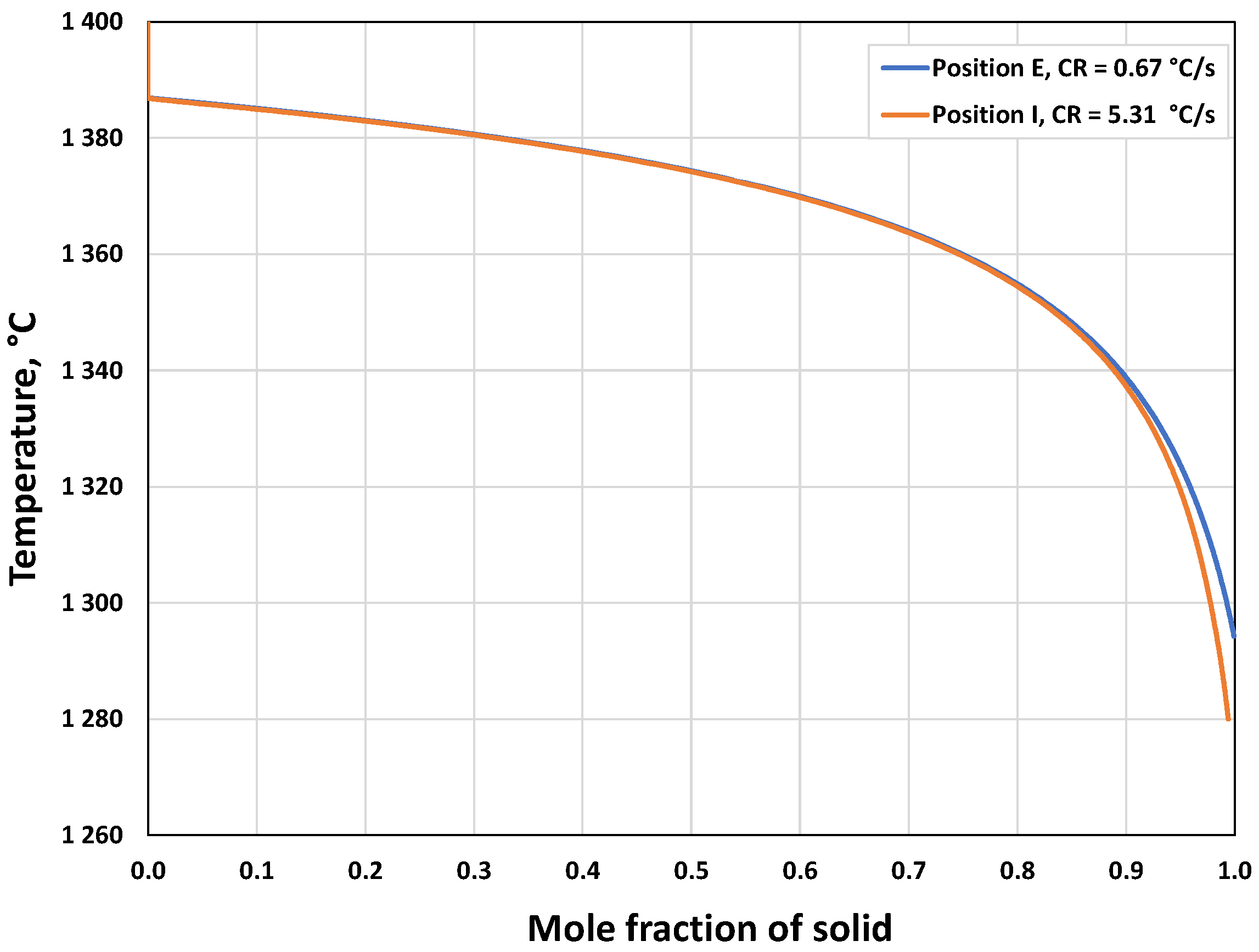
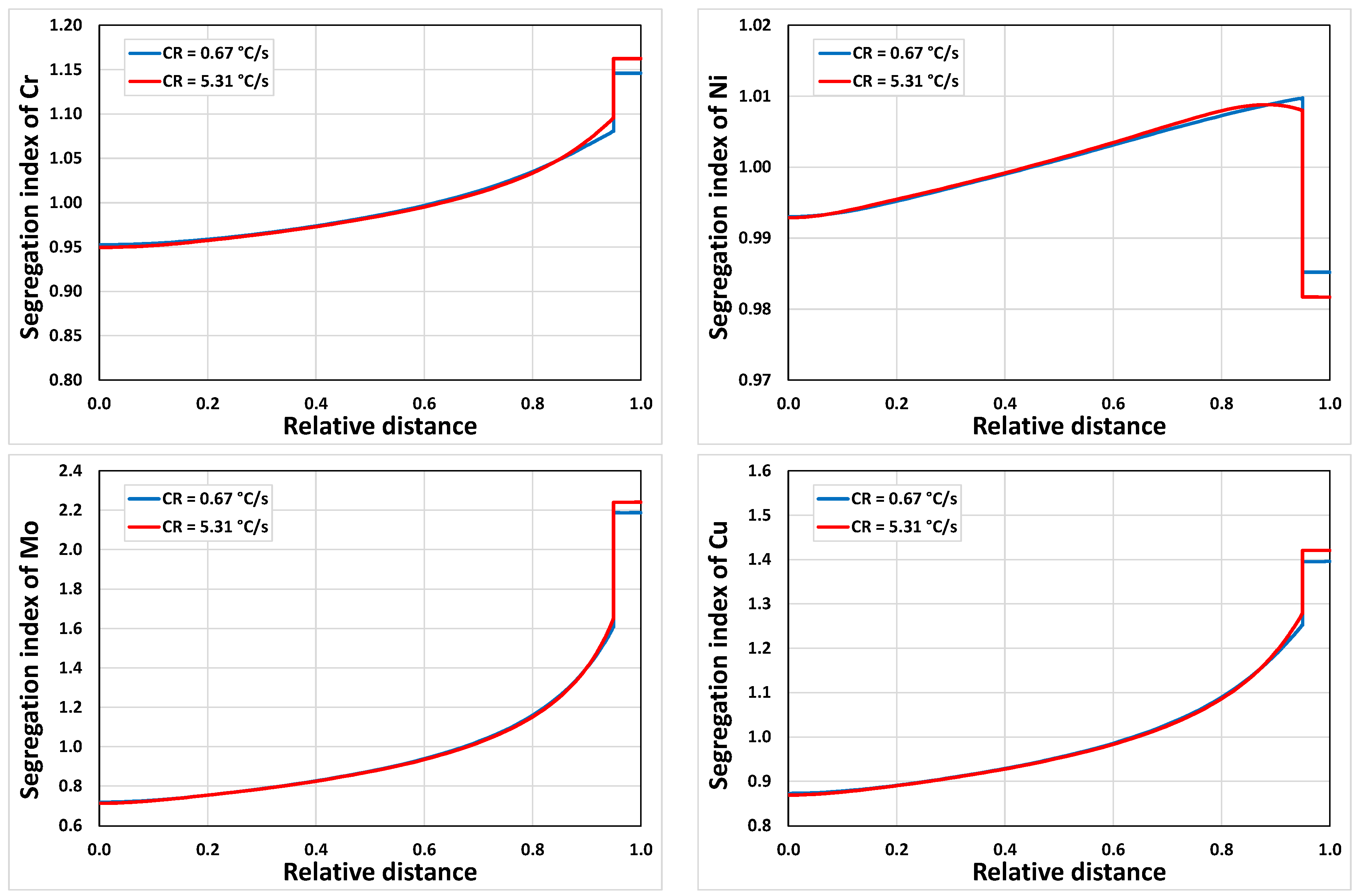
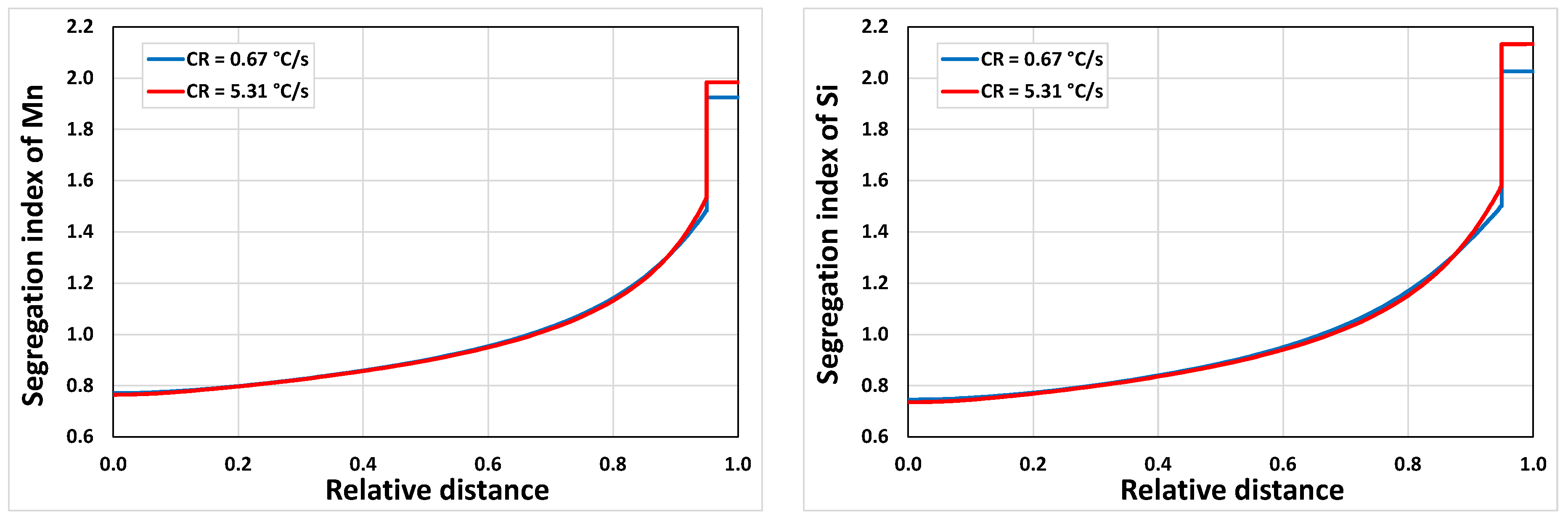
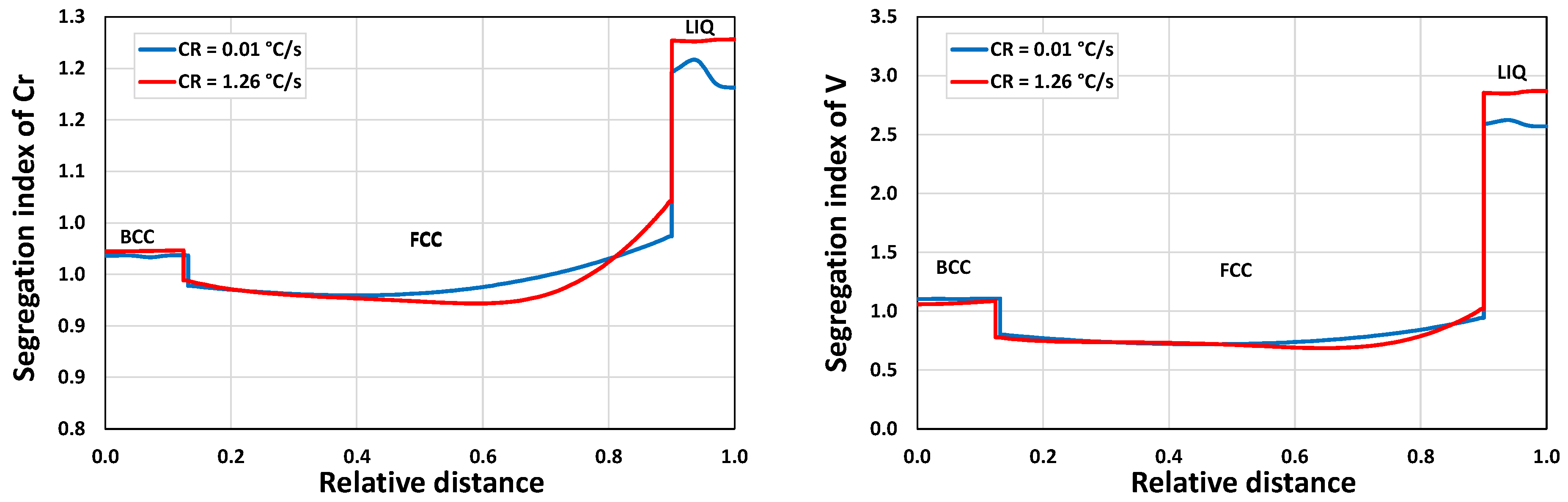
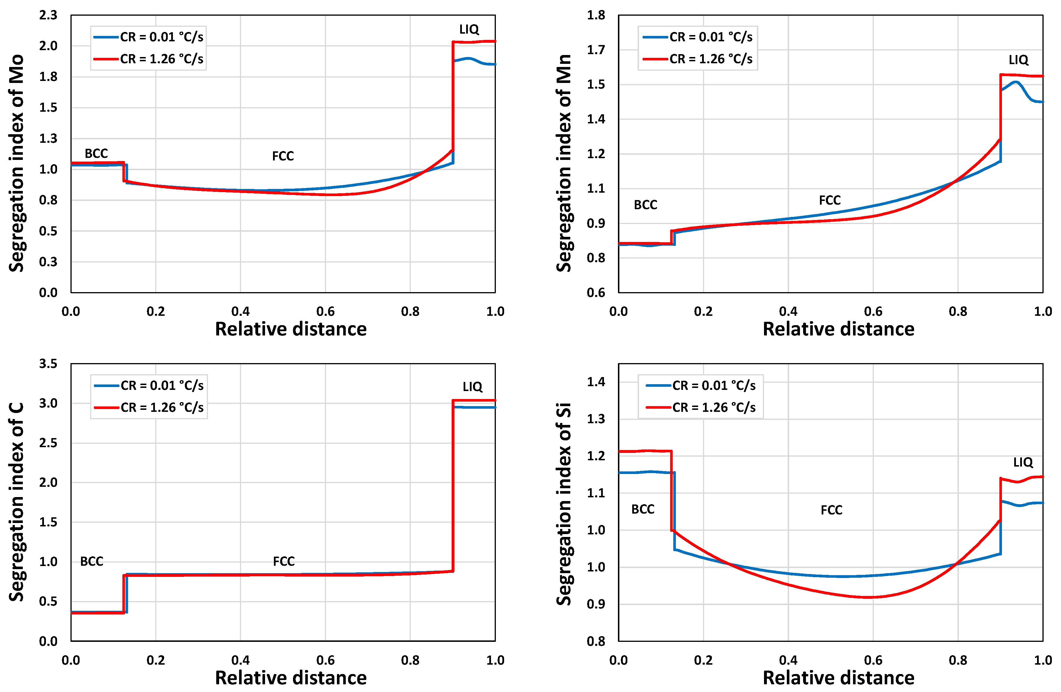
3.1.2. Microsegregation during Solidification

In MICAST, the segregation index for any element is used by defining a value C/C0. C is the locally measured concentration of a certain element and C0 is the bulk concentration of the same element. Segregation indexes of all elements for the stainless steel used just before final solidification are depicted in Figure 9. Even though carbon has the largest segregation index, it has little effect on the system due to its low content. The segregation index of carbon drops quickly after full solidification (Figure 10) as carbon can diffuse rapidly in the austenite. Carbon diffuses so rapidly that no obvious concentration gradient is found in the solid phase during solidification.
Mass percents of all elements for the tool steel used just after 0.4 s are depicted in Figure 11. The interfaces between BCC and FCC, as well as FCC and LIQUID, are moving towards the outside of the material when the temperature goes down, leading to a growing FCC into the liquid and BCC. This is a typical peritectic reaction as shown in Equation (8).
The mapping results of elements for the stainless steel are given in Figure 12, showing to some extent microsegregation of all elements.
Figure 13 shows the experimental and predicted concentration profiles of elements for the stainless steel used. It is found that nickel has lowest microsegregation and it is consistent with the segregation indexes shown in Figure 10. It should be noted that the nominal compositions result in larger deviations for Cr, Ni and Mn. Furthermore, the modified compositions (0.01 wt.%C, 0.33 wt.%Si, 0.37 wt.%Mn, 16.24 wt.%Cr, 17.33 wt.%Ni, 4.83 wt.%Mo, 1.58 wt.%Cu) based on the average value of the measured results were employed to generate new concentration profiles (red lines) which are close to the measured values (blue lines). As can be seen from Figure 13, the predicted microsegregations are generally consistent with the measured ones. Furthermore, the measured results show that the secondary dendrite arm spacing is somewhat irregular. The predicted peak value for the element Mn is larger than the measured peak. This may be due to slower diffusion of Mn in the calculation.
Experimentally obtained microstructure with concentrations of the elements Cr, V, Mn and Si for the tool steel used is revealed in Figure 14. Figure 15 shows the experimental and predicted concentration profiles of elements for the tool steel used. Despite the relatively large deviation between the measured and predicted concentrations (especially for Mn and Si), primarily due to the scattered measuring data, the predictions exhibit reasonable alignment with the average measured values.
In the current Section 3.1, two case studies were carried out for a general solidification study, corresponding to two steel grades (one stainless steel, one tool steel). The predicted microsegregation results agree with the measured ones for both cases. From the results in this section, feasible procedures are summarized to complete a general solidification analysis:
(1)
Equilibrium calculations using Thermo-Calc should be performed first to determine knowledge of possible phases over a reasonable range of temperatures. It also gives a picture regarding possible solidification reaction. An isopleth phase diagram provides basic information on equilibrium solidification path.
(2)
A Scheil calculation is carried out to obtain an overview of segregation of all elements quickly and possible phases during solidification.
(3)
A DICTRA setup model is created based on the information regarding phases and temperatures from both the equilibrium calculation and Scheil calculation as well as a calculation of domain size. DICTRA calculation is performed according to the specified cooling rate or given temperature–time curve.
(4)
A comparative analysis of experimental and calculated microsegregation is conducted.
Possible solidification paths are listed for the solidifying steel, which depend on chemical composition and cooling rate:
(A)
LL + δ ⇒ δ ⇒ γ + δ
(B)
LL + δ ⇒ L + γ + δ ⇒ γ + δ
(C)
LL + δ ⇒ L + γ + δ ⇒ γ
(D)
LL + γ ⇒ L + γ + σ
The modes (C) and (D) appear in the current work.

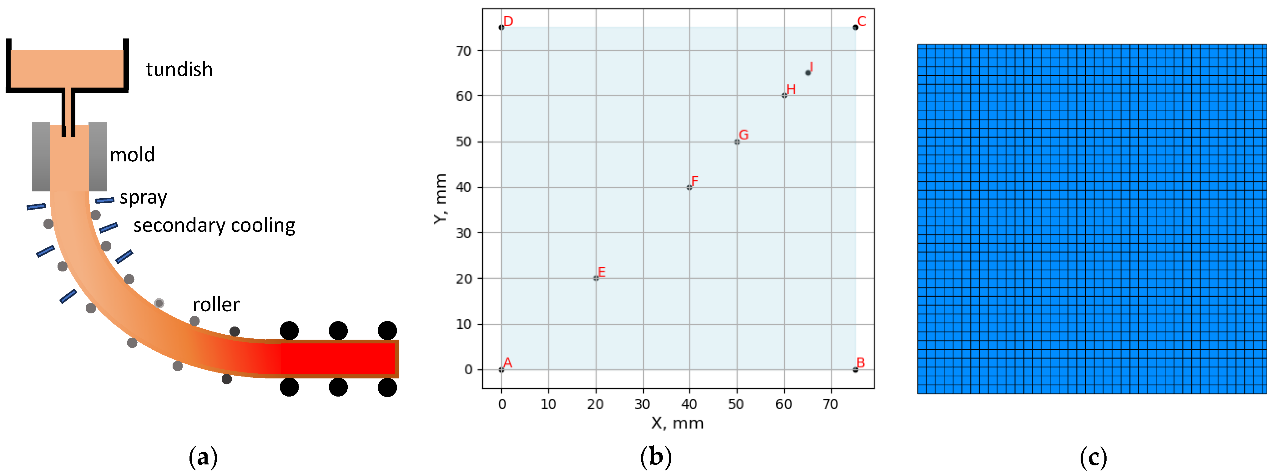
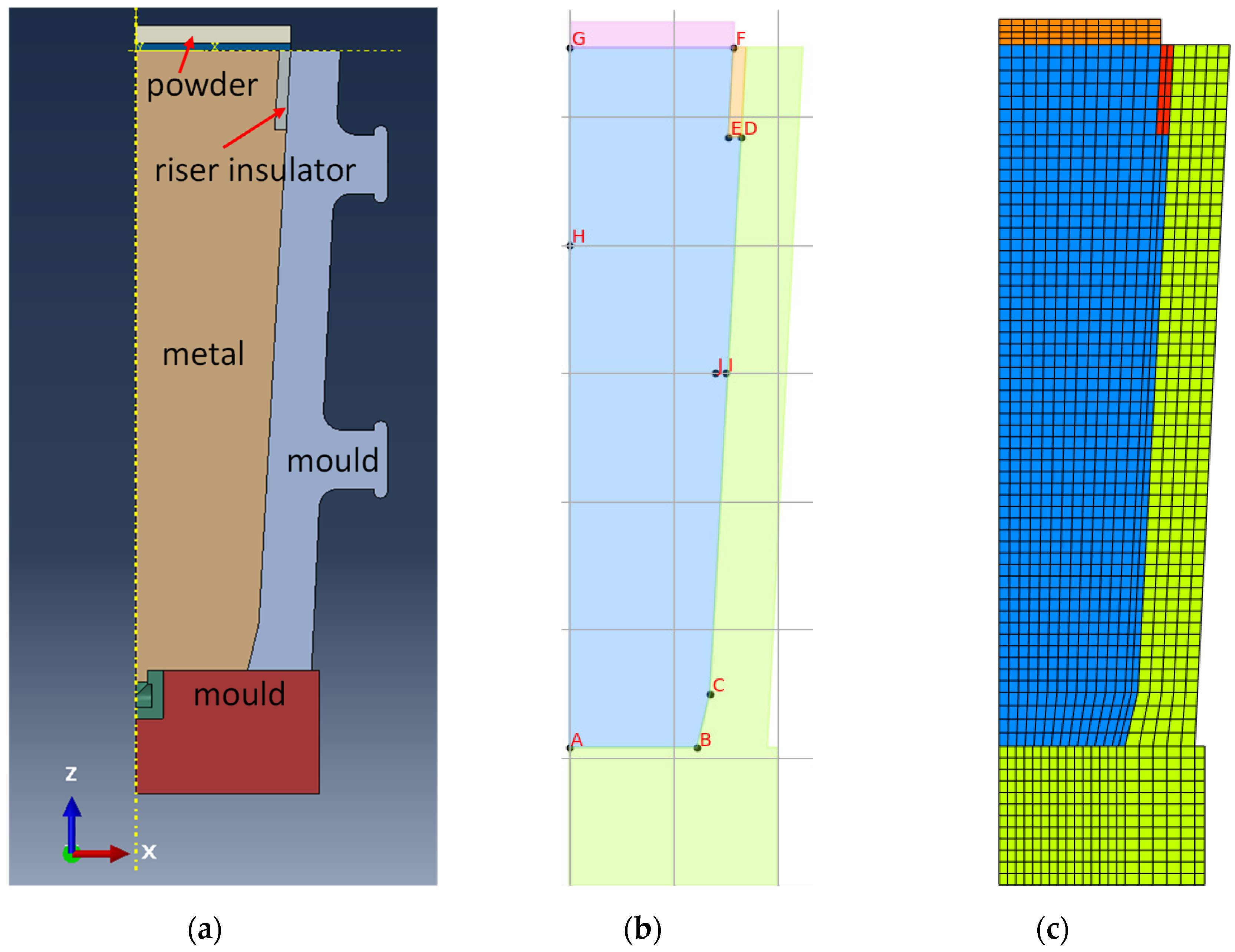
3.2. Solidification for Industrial Casting Process

Process simulations were performed by using Process simulation (CC) and Process simulation (IC) modules in MICAST for continuous casting (CC) and ingot casting (IC) processes, respectively. The solution for predicting the location-specific microstructures used in MICAST includes two steps: (1) to calculate temperature histories at the specific locations in the process simulations; (2) to build and run a DICTRA model to obtain microsegregations, etc.

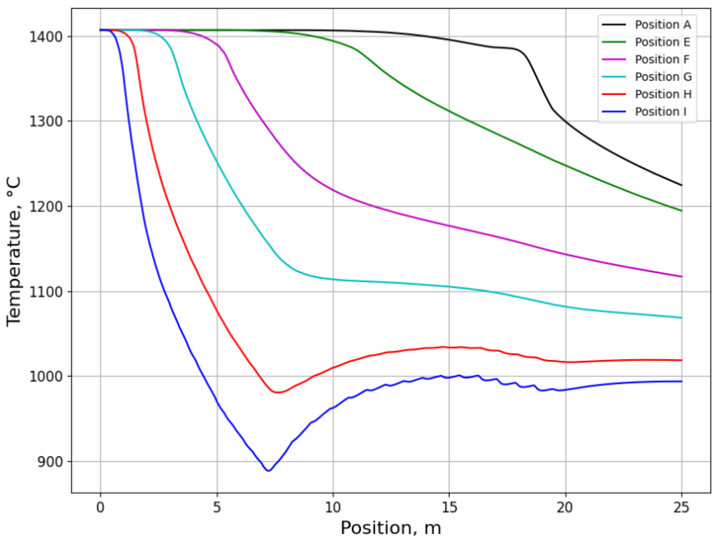
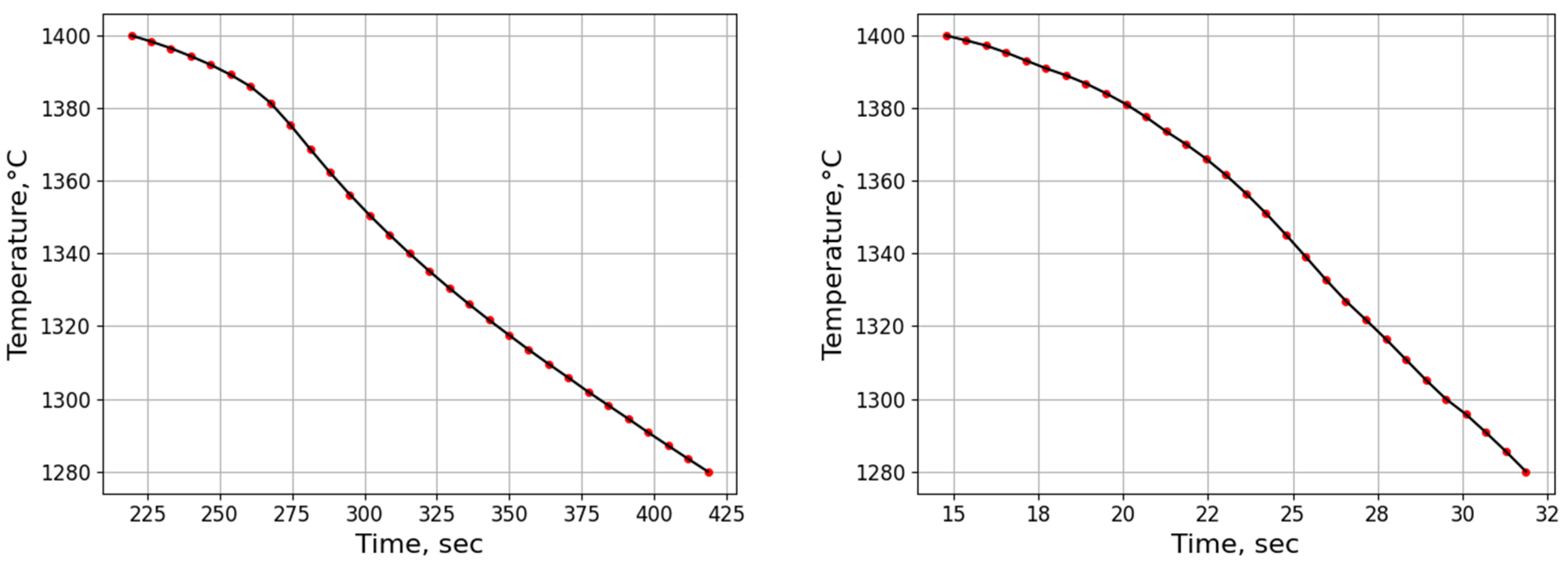
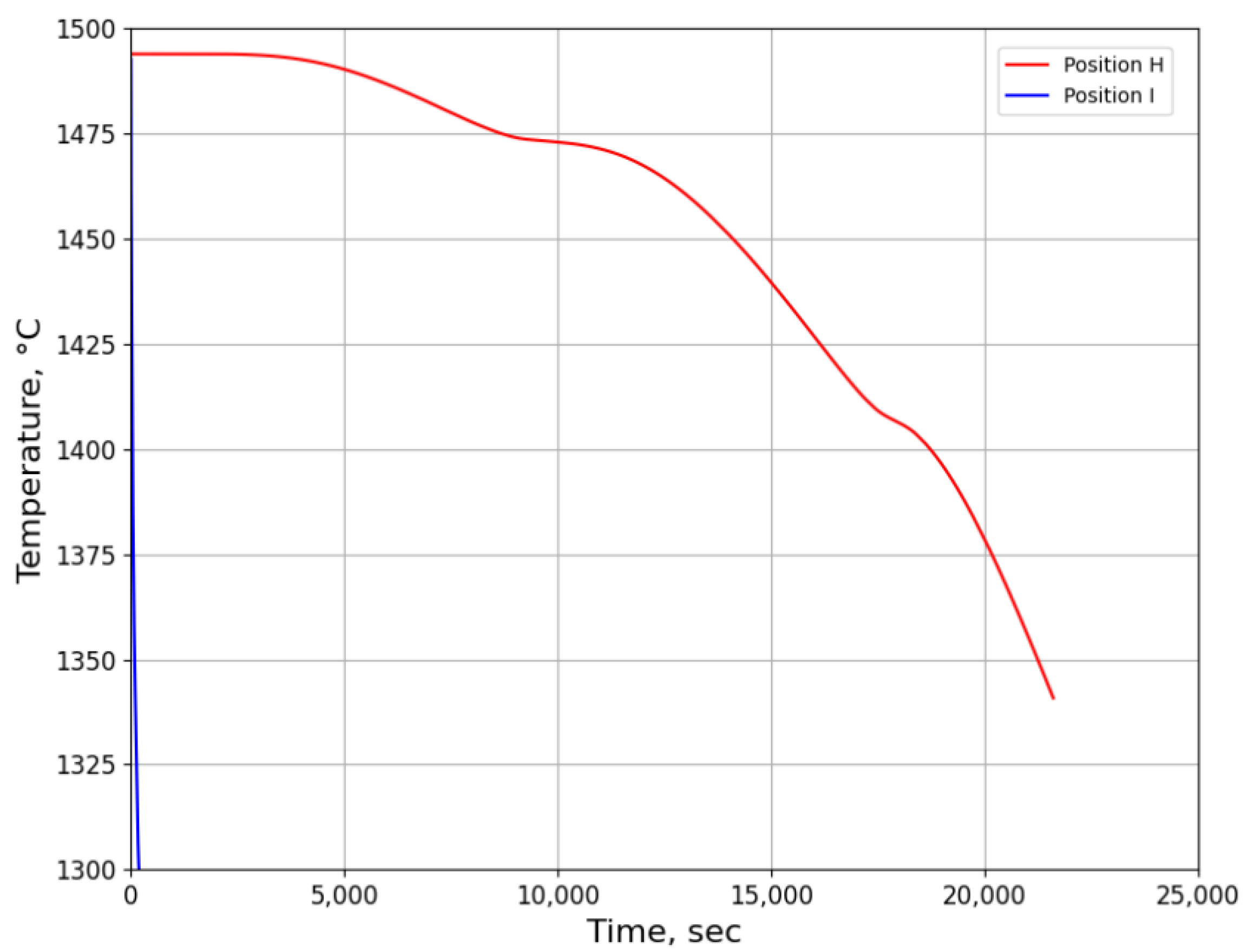
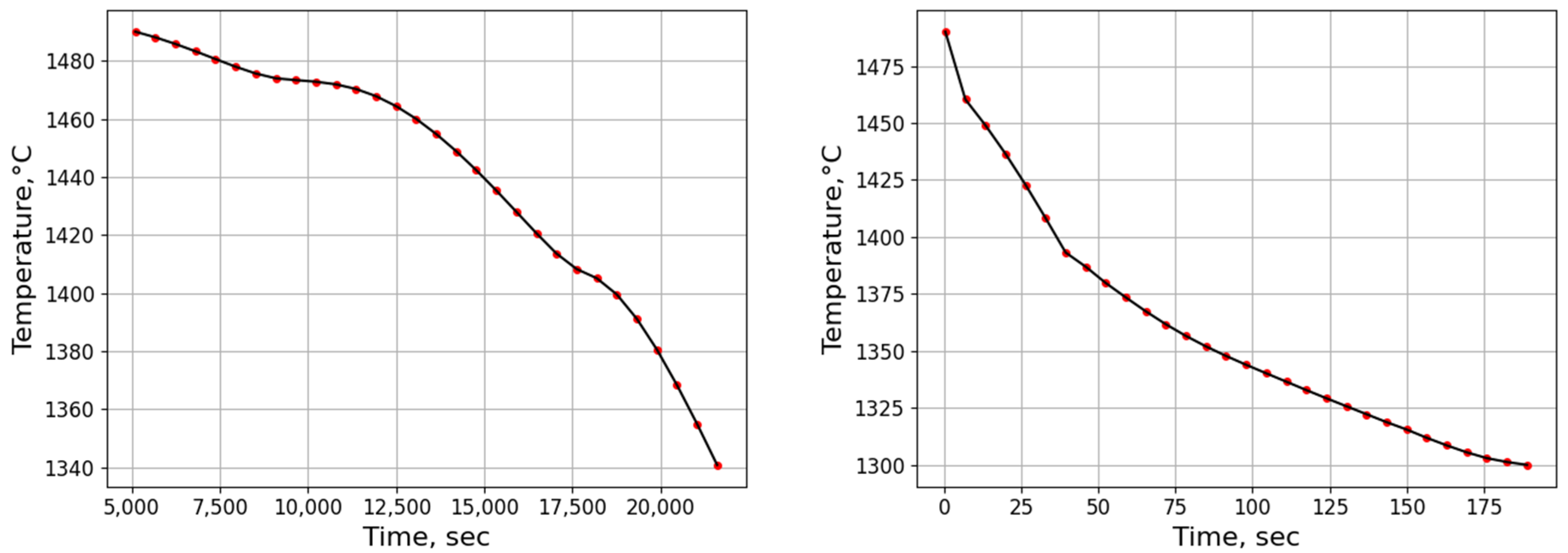
3.2.1. Temperature History from Process Simulation

In continuous casting (Figure 16a), the molten steel is cast in copper molds followed by secondary cooling. A case study for stainless steel (0.01 wt.%C, 0.35 wt.%Si, 1.7 wt.%Mn, 20 wt.%Cr, 25 wt.%Ni, 4.3 wt.%Mo, 1.5 wt.%Cu) was carried out for casting a 150 × 150 mm square billet with casting speed of 2.5 m/min.
Figure 16b,c shows the geometry with tracing points (from A to I) on the cross-section of cast strand and 2D finite element mesh, respectively. A quarter of the entire cross-section is selected for modelling. The cross-section is symmetric about X (AB) and Y (AD) axes with origin Point A. Point C is located at the corner. The cast machine in the present calculation was built according to real industrial technical data.
The calculated temperature–position curves at different tracing points (positions A, E, F, G, H, and I) are shown in Figure 17. The temperature evolution at the center point (position A) of the cross-section allows determination of the metallurgical length based on the full solidification.
An expression for secondary dendrite arm spacing is obtained by fitting data for stainless steel (steel 413: 0.01 wt.%C, 19 wt.%Cr, 25 wt.%Ni, 4 wt.%Mo, 1,5 wt.%Cu) from Jernkontoret [45]:
λ S D A S ( μ m ) = 66.193 T ˙ 0.26
where  T ˙    is the cooling rate (°C/s).
The time–temperature curves for positions E and I as shown in Figure 18 are exported as csv data files. The average cooling rates are calculated for temperatures ranging from liquidus temperature to solidus temperature as shown in Table 1. The corresponding secondary dendrite arm spacings are estimated using Equation (9).
The grid widths required for DICTRA simulation for cooling rates 5.31 °C/s and 0.67 °C/s are 22 μm and 37 μm, respectively, based on the dendrite arm spacings in Table 1. Two DICTRA models were generated using time–temperature data with a temperature range (1400 °C down to 1280 °C), estimated grid widths as well as solidification path (Equation (7)).
With ingot casting (Figure 19a), the molten steel from the steelworks solidifies in molds to form conical blocks, each with a mass up to several tons. A case study was carried out for a 2.9-ton ingot casting of tool steel (Fe-0.39 wt.%C-5.2 wt.%Cr-1.4 wt.%Mo-0.9 wt.%V-0.4 wt.%Mn-1.0 wt.%Si).
In the current model, only two-dimensional heat flow in a vertical section through the mid-width of the ingot is considered. Figure 19b,c shows the geometry with tracing points on the cross-section and 2D finite element mesh.
The variations of the temperature over time on the specified locations (positions H and I) are shown in Figure 20. The time–temperature curves are plotted in Figure 21 and the data are exported as csv data files. The average cooling rates are calculated for temperatures ranging from liquidus temperature to solidus temperature as shown also in Table 2. The corresponding secondary dendrite arm spacing is estimated using an empirical formula for H13 steel by Mao et al. [46]:
λ S D A S ( μ m ) = 46.93 · T ˙ 0.322
The measurements of secondary dendrite arm spacing for the samples from different locations in the tool steel used were conducted, ranging from 126.4 to 134.7 μm.
The grid widths required for DICTRA simulation for cooling rates 1.26 °C/s and 0.01 °C/s are 44 μm and 206 μm, respectively, based on the dendrite arm spacings in Table 2. Two DICTRA models were generated using the time–temperature data (Figure 21), dendrite arm spacing data (Table 2), as well as solidification path (Equation (8)).

3.2.2. Microsegregation Using Temperature History Data

Figure 22 shows the calculated solid fraction vs. temperature for positions E and I using DICTRA and precited temperature history data for the case of continuous casting of stainless steel. It is seen that the solidification follows the same path from the beginning and deviates from about 1350 °C, finishing with a higher solidus temperature for position E. It demonstrates that higher cooling rate may result in a lower solidus temperature.
Figure 23 shows the segregation indexes of all elements with different cooling rates at solidified fraction (0.95) in continuous casting of stainless steel. It is seen that cooling rate influences the microsegregation of elements, mostly in the final liquid pool in the inter-dendritic region. All elements are positively segregated in the solidified FCC close to the final liquid pool and in the final liquid pool, except for the element Ni which has negative segregation. The study [47] also reported a negative segregation of Ni from measurement by EPMA in a Fe–Cr–Ni–Mo–N super-austenitic stainless steel.
Figure 24 shows the calculated solid fraction vs. temperature for positions H and I using DICTRA and precited temperature history data for the case of ingot casting of tool steel. Again, a higher cooling rate results in a lower solidus temperature according to Figure 24. The calculated segregation indexes of all elements for the two positions (H and I) at solidified fraction (0.9) for the case of ingot casting of tool steel are shown in Figure 25. For all elements, higher cooling rates can cause severe segregation, especially in the remaining liquid pool.
The results of DICTRA simulation for positions H and I for the case of ingot casting of tool steel are also presented in Figure 26 and Figure 27, respectively. It is found that the fractions of austenite (γ) are slightly different at the temperature (around 1425.1 °C) for the two positions. In other words, austenite (γ) may form at a higher temperature for position H as the cooling rate is lower. The profiles of ferrite (δ) are obviously different for the two positions.
The corresponding animations for Figure 26 and Figure 27 are also available for interested readers, which illustrate the dynamic solidification process when the temperature falls from the liquidus temperature, showing a liquid fraction variation from 1 to 0 in the state bar (see the Supplementary Materials).
In the current Section 3.2, two case studies were performed for process simulations (continuous casting and ingot casting) with selected steel grades, mold geometry and process conditions using the finite element method.
From the process simulation practice, it may help to answer the following questions:
(1)
For continuous casting, what factors cause the biggest changes in the metallurgical length of the strand and the shell thickness under the mold?
(2)
For ingot casting, what factors cause the changes of full solidified time?
(3)
In which positions do the most pronounced microsegregation occur? How does it effectively trace the temperature history of the interested positions from the center to the surface below the meniscus?
The practice of the MICAST computational tool shows that the CALPHAD-based material models can be associated with the casting process model to predict the location-specific microstructures, so as to achieve the most efficient product manufacturing. This is conducted in the following procedures:
(1)
The temperature distributions and histories in continuous casting and ingot casting of steels were calculated using in-house finite-element code integrated in MICAST.
(2)
The predicted temperature history from the casting process simulation was exported as input data for the DICTRA simulation of solidification.
(3)
The resulting microsegregation by the DICTRA simulation will be compared with the measured ones if available. The measured microsegregation values at the specified locations are missing in the current paper and will be carried out in future work.

4. Conclusions

The following conclusions are drawn for this work:
(1)
Integrated computational materials engineering (ICME) of the industrial casting process can be achieved by incorporating macroscopic models (finite element-based thermal models) and microscopic models (CALPHAD-based microstructural models), building an industry-oriented computational tool (MICAST) for casting of steels. MICAST delivers a user-friendly interface which allows industrial users to start quickly.
(2)
Two case studies were performed for solidification simulations of tool steel and stainless steel by using the CALPHAD approach (Thermo-Calc package and CALPHAD database). The predicted microsegregation results agree with the measured ones. From the results in Section 3.1, feasible procedures are proposed to complete a general solidification analysis.
(3)
Two case studies were performed for process simulations (continuous casting and ingot casting) with selected steel grades, mold geometry and process conditions using the finite element method. The temperature distributions and histories in continuous casting and ingot casting of steels were calculated using in-house finite-element code integrated in MICAST. The predicted temperature history from the casting process simulation was exported as input data for the DICTRA simulation of solidification. The resulting microsegregation by the DICTRA simulation reflects the microstructure evolution in the real casting process. Current computational practice demonstrates that CALPHAD-based material models can be directly linked with casting process models to predict location-specific microstructures for smart material processing.
(4)
The animation of solidification sequence plus other outputs could be used as good pedagogical tools.

Supplementary Materials

The corresponding animations for Figure 26 and Figure 27 can be downloaded at: https://0-www-mdpi-com.brum.beds.ac.uk/article/10.3390/alloys2040021/s1.

Author Contributions

Conceptualization, C.L., K.H. and D.Å.; methodology, C.L.; software, C.L.; validation, K.H. and D.Å.; formal analysis, C.L., Z.S. and F.C.; investigation, C.L., K.H., Z.S., D.Å., E.S.P., F.C. and C.X.; resources, K.H., D.Å. and E.S.P.; data curation, C.L.; writing—original draft preparation, C.L.; writing—review and editing, C.L., K.H., Z.S., D.Å., E.S.P. and F.C.; visualization, C.L.; supervision, K.H. and E.S.P.; project administration, C.L.; funding acquisition, C.L., K.H. and D.Å. All authors have read and agreed to the published version of the manuscript.

Funding

The authors kindly acknowledge VINNOVA—Swedish Governmental Agency for Innovation Systems for financial support of the research within the Material-based Competitiveness program (grant number: 2018-02578).

Data Availability Statement

The data are not publicly available.

Acknowledgments

This project is carried out in collaboration among Swerim AB, Alleima AB and Uddeholms AB. The authors thank Fatemeh Shahbazian (former researcher at Swerim AB) for helpful discussions.

Conflicts of Interest

The authors declare no conflict of interest.

References

  1. Flemings, M.C. Solidification Processing; McGraw-Hill Book Company: New York, NY, USA, 1974. [Google Scholar]
  2. Kurz, W.; Fisher, D.J. Fundamentals of Solidification, 4th ed.; Trans Tech Publications: Aedermannsdorf, Switzerland, 1998. [Google Scholar]
  3. Fredriksson, H.; Ulla, A. Materials Processing during Casting; Wiley: Chichester, UK, 2006; Volume 210. [Google Scholar]
  4. Dantzig, J.A.; Rappaz, M. Solidification; EPFL Press: Lausanne, Switzerland, 2009. [Google Scholar]
  5. Cabrera-Marrero, J.M.; Carreno-Galindo, V.; Morales, M.; Chavez-Alcala, F. Macro-micro modeling of the dendritic microstructure of steel billets processed by continuous casting. ISIJ Int. 1998, 50, 812–821. [Google Scholar] [CrossRef]
  6. Celentano, D.J.; Dardati, P.M.; Godoy, L.A.; Boeri, R.E. Computational simulation of microstructure evolution during solidification of ductile cast iron. Int. J. Cast Met. Res. 2008, 21, 416–426. [Google Scholar] [CrossRef]
  7. Bellon, B.; Boukellal, A.K.; Isensee, T.; Wellborn, O.M.; Trumble, K.P.; Krane, M.J.M.; Titus, M.S.; Tourret, D.; Llorca, J. Multiscale prediction of microstructure length scales in metallic alloy casting. Acta Mater. 2021, 207, 116686. [Google Scholar] [CrossRef]
  8. Cusato, N.; Nabavizadeh, S.A.; Eshraghi, M. A Review of Large-Scale Simulations of Microstructural Evolution during Alloy Solidification. Metals 2023, 13, 1169. [Google Scholar] [CrossRef]
  9. Chen, Z.; Li, Y.; Zhao, F.; Li, S.; Zhang, J. Progress in numerical simulation of casting process. Meas. Control. 2022, 55, 257–264. [Google Scholar] [CrossRef]
  10. Wu, M.; Ludwig, A.; Kharicha, A. Simulation of As-Cast Steel Ingots. Steel Res. Int. 2018, 89, 1700037. [Google Scholar] [CrossRef]
  11. Thomas, B.G. Review on modeling and simulation of continuous casting. Steel Res. Int. 2017, 89, 1700312. [Google Scholar] [CrossRef]
  12. Miłkowska-Piszczek, K.; Falkus, J. Control and design of the steel continuous casting process based on advanced numerical models. Metals 2018, 8, 591. [Google Scholar] [CrossRef]
  13. Demay, C.; Ferrand, M.; Belouah, S.; Robin, V. Modeling and simulation of ingot solidification with the open-source software Code_Saturne. IOP Conf. Ser. Mater. Sci. Eng. 2020, 861, 012033. [Google Scholar] [CrossRef]
  14. Khan, M.A.A.; Sheikh, A.K. A comparative study of simulation software for modelling metal casting processes. Int. J. Simul. Model. 2018, 17, 197–209. [Google Scholar] [CrossRef]
  15. Kamal, M.; Sahai, Y. Modeling of melt flow and surface standing waves in a continuous casting mold. Steel Res. Int. 2005, 76, 44–52. [Google Scholar] [CrossRef]
  16. Hepp, E.; Bernbeck, P.; Schäfer, W.; Senk, D. New Developments for Process Modelling of the Continuous Casting of Steel. In SteelSim 2007; Graz: Seggau, Austria, 2007; p. 203. [Google Scholar]
  17. Li, W.M.; Jiang, Z.H.; Li, H.B. Simulation and Calculation to Segregation of High Nitrogen Steels Solidification Process Based on PROCAST Software. Adv. Mater. Res. 2011, 217, 1185–1190. [Google Scholar] [CrossRef]
  18. Burbelko, A.; Falkus, J.; Kapturkiewicz, W.; Sołek, K.; Drożdż, P.; Wróbel, M. Modeling of the grain structure formation in the steel continuous ingot by CAFE method. Arch. Metall. Mater. 2012, 57, 379–384. [Google Scholar] [CrossRef]
  19. Patil, P.; Puranik, A.; Balachandran, G.; Balasubramanian, V. Improvement in Quality and Yield of the Low Alloy Steel Ingot Casting Through Modified Mould Design. Trans. Indian Inst. Met. 2017, 70, 2001–2015. [Google Scholar] [CrossRef]
  20. Zhang, C.; Shahriari, D.; Loucif, A.; Jahazi, M.; Lapierre-Boire, L.P.; Tremblay, R. Effect of segregated alloying elements on the high strength steel properties: Application to the large size ingot casting simulation. In TMS 2017 146th Annual Meeting & Exhibition Supplemental Proceedings; Springer International Publishing: Cham, Switzerland, 2017; pp. 491–500. [Google Scholar]
  21. Fang, Q.; Ni, H.; Zhang, H.; Wang, B.; Liu, C. Numerical study on solidification behavior and structure of continuously cast U71Mn steel. Metals 2017, 7, 483. [Google Scholar] [CrossRef]
  22. Kotásek, O.; Kurka, V.; Vindyš, M.; Jonšta, P.; Noga, R.; Dobiáš, M. Comparison of casting and solidification of 12 ton steel ingot using two different numerical software. In Proceedings of the 30th Anniversary International Conference on Metallurgy and Materials, Brno, Czech Republic, 26–28 May 2021; pp. 147–152. [Google Scholar]
  23. CALPHAD. Available online: https://en.wikipedia.org/wiki/CALPHAD (accessed on 23 November 2023).
  24. Sarreal, J.A.; Abbaschian, G.J. The effect of solidification rate on microsegregation. Metall. Trans. A 1986, 17, 2063–2073. [Google Scholar] [CrossRef]
  25. Won, Y.M.; Thomas, B.G. Simple model of microsegregation during solidification of steels. Metall. Mater. Trans. A 2001, 32, 1755–1767. [Google Scholar] [CrossRef]
  26. Poirier, D.R.; Heinrich, J.C. Modeling of Microsegregation and Macrosegregation, Casting; ASM Handbook; ASM International: Materials Park, OH, USA, 2008; Volume 15, pp. 445–448. [Google Scholar]
  27. Natsume, Y.; Shimamoto, M.; Ishida, H. Numerical modeling of microsegregation for Fe-base multicomponent alloys with peritectic transformation coupled with thermodynamic calculations. ISIJ Int. 2010, 50, 1867–1874. [Google Scholar] [CrossRef]
  28. Zhang, D. Characterisation and Modelling of Segregation in Continuously Cast Steel Slab. Ph.D. Thesis, University of Birmingham, Birmingham, UK, 2015. Available online: https://etheses.bham.ac.uk/id/eprint/6256/ (accessed on 23 November 2023).
  29. Kobayashi, Y.; Todoroki, H.; Mizuno, K. Problems in solidification model for microsegregation analysis of Fe–Cr–Ni–Mo–Cu alloys. ISIJ Int. 2019, 59, 277–282. [Google Scholar] [CrossRef]
  30. Zhang, C.; Jahazi, M.; Isabel Gallego, P. On the Impact of Microsegregation model on the thermophysical and solidification behaviors of a large size steel ingot. Metals 2020, 10, 74. [Google Scholar] [CrossRef]
  31. Thermo-Calc Application Example: Microsegregation during Solidification. Available online: https://thermocalc.com/showcase/application-examples/microsegregation-during-solidification/ and https://thermocalc.com/wp-content/uploads/Application_Examples/Microsegregation_Solidification/analysis-of-microsegregation-during-solidification.pdf (accessed on 23 November 2023).
  32. ICME. Available online: https://en.wikipedia.org/wiki/Integrated_computational_materials_engineering (accessed on 23 November 2023).
  33. Luo, A.A. Material design and development: From classical thermodynamics to CALPHAD and ICME approaches. Calphad 2015, 50, 6–22. [Google Scholar] [CrossRef]
  34. Zhang, C.; Miao, J.; Chen, S.; Zhang, F.; Luo, A.A. CALPHAD-Based Modeling and Experimental Validation of Microstructural Evolution and Microsegregation in Magnesium Alloys During Solidification. J. Phase Equilibria Diffus. 2019, 40, 495–507. [Google Scholar] [CrossRef]
  35. Luo, C.; Antonsson, K.H.; Shahbazian, F. An Industry Oriented Computational Tool for Modelling Microstructure in Continuous Casting of Steel (MICAST I), Swerea KIMAB AB internal report; Stockholm, Sweden, 2017.
  36. Luo, C.; Shahbazian, F.; Antonsson, K.H.; Song, Z.; Karlsson, L.; Ågren, D.; Persson, E.; Cederholm, F.; Xuan, C.; Ejnermark, S. An Industry Oriented Computational Tool for Modelling Microstructure in Casting of Steel (MICAST II), Swerim AB report (No. MEF21181); Stockholm, Sweden, 2021.
  37. Kaufman, L.; Bernstein, H. Computer Calculation of Phase Diagrams; Academic Press: New York, NY, USA, 1970; ISBN 0-12-402050-X. [Google Scholar]
  38. CALPHAD. Available online: https://CALPHAD.org.
  39. Gulliver, G.H. The quantitative effect of rapid cooling upon the constitution of binary alloys. J. Inst. Met. 1913, 9, 120–157. [Google Scholar]
  40. Scheil, E. Remarks on the crystal layer formation. Z. Metallkd. 1942, 34, 70. [Google Scholar]
  41. Thermo-Calc Software. Available online: https://thermocalc.com/.
  42. Schematic of Scheil–Gulliver model. Available online: https://en.wikipedia.org/wiki/Scheil_equation (accessed on 23 November 2023).
  43. Ågren, J. Numerical treatment of diffusional reactions in multicomponent alloys. J. Phys. Chem. Solids 1982, 43, 385–391. [Google Scholar] [CrossRef]
  44. Miettinen, J.; Louhenkilpi, S.; Kytönen, H.; Laine, J. IDS: Thermodynamic–kinetic–empirical tool for modelling of solidification, microstructure and material properties. Math. Comput. Simul. 2010, 80, 1536–1550. [Google Scholar] [CrossRef]
  45. Jernkontoret. A Guide to the Solidification of Steels; Jernkontoret, Stockholm, Sweden. 1977. Available online: https://www.phase-trans.msm.cam.ac.uk/2007/Solidification/solidification.html (accessed on 23 November 2023).
  46. Mao, M.; Guo, H.; Wang, F.; Sun, X. Effect of cooling rate on the solidification microstructure and characteristics of primary carbides in H13 steel. ISIJ Int. 2019, 59, 848–857. [Google Scholar] [CrossRef]
  47. Hao, Y.; Cao, G.; Li, C.; Liu, W.; Li, J.; Liu, Z.; Gao, F. Solidification structures of Fe–Cr–Ni–Mo–N super-austenitic stainless steel processed by twin-roll strip casting and ingot casting and their segregation evolution behaviors. ISIJ Int. 2018, 58, 1801–1810. [Google Scholar] [CrossRef]
Figure 1. Schematic of Scheil–Gulliver model [42].
Alloys 02 00021 g001
Figure 2. (a) Solidification path for AISI 314 stainless steel during solidification using both Scheil model and DICTRA; (b) Micro segregation of elements in the liquid phase during solidification using Scheil model.
Alloys 02 00021 g002
Figure 3. Schematic diagram for CALPHAD-based ICME approach on a MICAST platform.
Alloys 02 00021 g003
Figure 4. Linkage between FEM and CALPHAD tools.
Alloys 02 00021 g004
Figure 5. Calculated solid fraction vs. temperature using Scheil and DICTRA for solidification of the stainless steel used: (a) comparison using DICTRA and Scheil; (b) detailed phases using Scheil.
Alloys 02 00021 g005
Figure 6. Fe–Ni isopleth phase diagram for the stainless steel.
Alloys 02 00021 g006
Figure 7. Calculated solid fraction vs. temperature using Scheil and DICTRA for solidification of the tool steel: (a) comparison using DICTRA and Scheil; (b) detailed phases using Scheil.
Alloys 02 00021 g007
Figure 8. Stable Fe–C isopleth phase diagram for the tool steel.
Alloys 02 00021 g008
Figure 9. Segregation indexes of all elements just before final solidification (57.8 s, solid fraction 0.88, temperature 1354 °C) for the stainless steel.
Alloys 02 00021 g009
Figure 10. Segregation indexes of all elements after final solidification (125 s, temperature 1287 °C) for stainless steel.
Alloys 02 00021 g010
Figure 11. Concentration profiles of all elements just after 0.4 s (corresponding to a solid fraction of 0.76, temperature 1440 °C) for the tool steel.
Alloys 02 00021 g011
Figure 12. EPMA mapping of elements for the stainless steel.
Alloys 02 00021 g012
Figure 13. Experimental and predicted concentration profiles of elements for the stainless steel.
Alloys 02 00021 g013aAlloys 02 00021 g013b
Figure 14. Microstructure with secondary dendrite arms of tool steel after solidification. A yellow line is used to measure the concentration profiles of elements.
Alloys 02 00021 g014
Figure 15. Experimental and predicted concentration profiles of elements for the tool steel.
Alloys 02 00021 g015
Figure 16. (a) Schematic diagram of continuous casting; (b) geometry with tracing points (A, B, C, D, E, F, G, H, I) on the cross-section of 150 mm × 150 mm billet; (c) 2D finite element mesh.
Alloys 02 00021 g016
Figure 17. The temperature histories at the selected points from continuous casting of stainless steel billet.
Alloys 02 00021 g017
Figure 18. Time–temperature curves at the selected positions (E and I) for continuous casting case.
Alloys 02 00021 g018
Figure 19. (a) Schematic diagram of ingot casting; (b) geometry with tracing points on the vertical cross-section; (c) 2D finite element mesh.
Alloys 02 00021 g019
Figure 20. Time—temperature curves at the selected position (H and I) for ingot casting case.
Alloys 02 00021 g020
Figure 21. Time–temperature curves at the selected positions (H and I) for ingot casting case.
Alloys 02 00021 g021
Figure 22. Calculated solid fraction vs. temperature with different cooling rates for positions E and I, respectively in continuous casting of stainless steel.
Alloys 02 00021 g022
Figure 23. Segregation indexes of all elements using different cooling curves at solidified fraction (0.95) in continuous casting of stainless steel.
Alloys 02 00021 g023aAlloys 02 00021 g023b
Figure 24. Calculated solid fraction vs. temperature with different cooling rates for positions E and I, respectively in ingot casting of tool steel.
Alloys 02 00021 g024
Figure 25. Segregation indexes of all elements for the two positions (H and I) at solidified fraction (0.9) in ingot casting of tool steel.
Alloys 02 00021 g025aAlloys 02 00021 g025b
Figure 26. The results of DICTRA simulation for position H in ingot casting of tool steel.
Alloys 02 00021 g026
Figure 27. The results of DICTRA simulation for position I in ingot casting of tool steel.
Alloys 02 00021 g027
Table 1. Averaged cooling rates for positions E and I during solidification range of continuous casting, dendrite arm spacing calculated by Equation (9).
Position Average Cooling Rate (°C/s)Dendrite Arm Spacing (μm)
E0.6774
I5.3144
Table 2. Averaged cooling rates for positions H and I during solidification range of ingot casting, dendrite arm spacing calculated by Equation (10).
Position Average Cooling Rate (°C/s)Dendrite Arm Spacing (μm)
H0.01206
I1.2644
Disclaimer/Publisher’s Note: The statements, opinions and data contained in all publications are solely those of the individual author(s) and contributor(s) and not of MDPI and/or the editor(s). MDPI and/or the editor(s) disclaim responsibility for any injury to people or property resulting from any ideas, methods, instructions or products referred to in the content.

