Uncovering Discrete Non-Linear Dependence with Information Theory

Abstract

In this paper, we model discrete time series as discrete Markov processes of arbitrary order and derive the approximate distribution of the Kullback-Leibler divergence between a known transition probability matrix and its sample estimate. We introduce two new information-theoretic measurements: information memory loss and information codependence structure. The former measures the memory content within a Markov process and determines its optimal order. The latter assesses the codependence among Markov processes. Both measurements are evaluated on toy examples and applied on high frequency foreign exchange data, focusing on 2008 financial crisis and 2010/2011 Euro crisis.

1. Introduction

A century ago Markov [1] introduced a computational technique for time series that is now famously known as Markov processes. The transitions from one state to the other are modeled as a stochastic process, whereas the transition probabilities to the next state in the time series only depend on the preceding states. The number of preceding states that the transition probabilities depend on is referred to as the order of the process. Now, there is an active and diverse interdisciplinary community of researchers using Markov processes in computer science [2], statistics [3], pattern recognition [4], finance [5] and many other areas.

In practice, both the transition probabilities and the order of the Markov process are unknown, hence there arises the problem of making inferences about them from empirical data. In the last few decades there has been a great number of research on estimation of the optimal order of a Markov process [6,7]. The two most popular methods are Akaike information criterion (AIC) [8] and Bayesian information criterion (BIC) [9]. Both methods use the likelihood ratio statistics for model comparison and modify it by a penalty term. AIC has had a fundamental impact in statistical model evaluation problems and has been applied to the problem of estimating the order of autoregressive processes and Markov processes. The estimator was derived as an asymptotic estimate of the Kullback-Leibler divergence and provides a useful tool for evaluating models estimated by the maximum likelihood method. AIC is the most used and successful estimator of the optimal order of Markov process at the present time, as it performs better than BIC estimator for samples of relatively small size. On the other hand, both AIC and BIC do not provide a test of a model in the sense of testing a null hypothesis, i.e., they can tell nothing about the quality of the model in an absolute sense. Order selection is heuristic as the methods do not directly minimize a certain measure of the error between the order estimate and the true order, and the order estimator is usually defined as the minimizing value of this information criterion. In [7,10], different statistical techniques have been developed to test different assumptions about the order of the Markov process. For example, [10] develop a χ² test to test that a Markov process is of a given order against a larger order. In particular, with it we can test the hypothesis that a process has rth-order against (r + 1)th-order, until the test rejects the null hypothesis and then choose the last r as the optimal order. The statistical tests for optimal order of Markov process from information theoretic perspective are currently missing and in this paper we fill that gap.

Very often, one has to consider multiple Markov processes (data sequences) at the same time. This is because very often processes (sequences) can be correlated and therefore the information of other processes can contribute to the process considered. Thus by exploring these relationships, one can develop better models for better prediction rules. In view of this, [12] proposed a first-order multivariate Markov process model. In [13], a multivariate Markov process model is used to build stochastic networks for gene expression sequences. An application of the multivariate Markov process model to modelling credit risk has been also discussed in [14]. A topic that has attracted little attention concerns the identification of co-dependence among Markov processes. As discrete Markov processes can be simultaneously observed and modeled, there is a natural desire to evaluate the transition probability matrix of the joint Markov process to infer if the processes have co-dependences among them.

In this paper we model discrete time series as discrete Markov process of arbitrary order. We derive the approximate distribution of Kullback-Leibler divergence between a known transition probability matrix and its sample estimate, as a sum of gamma distributed random variables. We present the procedure for Markov process extension that allows comparison of processes of different order and define an information theoretic measurement termed information memory loss which evaluates the memory content within time series and provides an information theoretic method to determine the optimal order of Markov process. Finally, we present the construction of the so-called structureless transition probability matrix that models codependence among processes and define an information theoretic measurement termed information codependence structure which measures the co-dependence among Markov processes. Both measurement are validated on toy examples and evaluated on high frequency foreign exchange (FX) data, finding that the presented measurements are successful in detecting changes in memory of time series and breakdown of co-dependence among time series.

The rest of this paper is organized as follows; in Section 2 we derive the distribution of Kullback-Leibler divergence. Section 3 defines information memory loss, that describes the memory within time series. Section 4 describes information codependence structure that measures the co-dependence among Markov processes.

2. Kullback-Leibler Divergence Distribution

In this section we derive the distribution of an information theoretic measurement between two Markov processes. We present the definition of Kullback-Leibler divergence, an information theoretic measurement between two discrete probability distributions. Next, we present the Kullback-Leibler divergence for discrete Markov processes. Finally, we derive the distribution of Kullback-Leibler divergence between known transition probability matrix and its sample estimate.

In information theory, the Kullback-Leibler divergence [15] is used as a non-symmetric measure of the difference between two probability distributions. The Kullback-Leibler divergence of probability distribution ℚ from probability distribution ℙ, denoted ${\mathcal{D}}_{KL}(\mathbb{P}\parallel \mathbb{Q})$, is a measure of the information lost when ℚ is used to approximate ℙ. The probability measure ℙ represents the “true” distribution of data, while the probability measure ℚ typically represents a model or approximation of ℙ. For discrete probability distributions ℙ and ℚ, both on (Ω, $ℱ$), the Kullback-Leibler divergence of ℚ from ℙ, is defined as

$${\mathcal{D}}_{KL}(\mathbb{P}\parallel \mathbb{Q})={\displaystyle \sum _{\omega \in \mathrm{\Omega }}\log }\left(\frac{\mathbb{P}(\omega )}{\mathbb{Q}(\omega )}\right)\mathbb{P}(\omega )$$

(1)

If the probability distributions coincide then the resulting Kullback-Leibler divergence of ℚ from ℙ equals zero.

Before presenting the Kullback-Leibler divergence for discrete Markov processes we present the notation. The state space of a Markov process is denoted with $\mathcal{S}$, the states are denoted with $s\in \mathcal{S}$, and the corresponding transition probability matrix with W. As a shorthand, we write the first order transition probability from state s_j to state s_i as

$$\mathbb{P}(s_j\to s_i)$$

(2)

In case the transition dynamics is modeled as a k-th order Markov process, the transition probabilities is denoted as

$$\mathbb{P}((s_{i_k}\to \cdots \to s_{i_1})\to s_i)$$

(3)

indicating the transition to state s_i is conditioned on the history of previous k transitions $s_{i_k}\to \cdots \to s_{i_1}$. If the history of the previous transitions is known from the context or is irrelevant, we denote the previous k transitions with $S_i=(s_{i_k}\to \cdots \to s_{i_1})\in {\mathcal{S}}^k$, and the resulting transition probabilities of the k-th order Markov process with

$$W=[\mathbb{P}(S_i\to s_i)]S_i\in {\mathcal{S}}^k,s_i\in \mathcal{S}$$

(4)

Now we recall that the Kullback-Leibler divergence between two discrete Markov processes [17] for state space ${\mathcal{S}}^k=\{S_1,\dots ,S_M\}$ and transition probability matrices W and Ŵ of Markov processes of order k, equals

$$\begin{array}{l}{\mathcal{D}}_{KL}(W\parallel \widehat{W})={\displaystyle \sum _{i=1}^M{\mu }_{S_i}{\mathcal{D}}_{KL}}({\mathbb{P}}_{S_i}\parallel {\mathbb{Q}}_{S_i})\\ ={\displaystyle \sum _{i=1}^M{\mu }_{S_i}}\left[{\displaystyle \sum _{j=1}^{l_i}\log \left(\frac{\mathbb{P}(S_i\to s_{i_j})}{\mathbb{Q}(S_i\to s_{i_j})}\right)\mathbb{P}}(S_i\to s_{i_j})\right]\end{array}$$

(5)

where $\mathrm{\mu }=({\mathrm{\mu }}_{S_1},\dots ,{\mathrm{\mu }}_{S_M})$ is the stationary distribution corresponding to W, M is the number of states, while l_i is the number of possible transitions from state S_i, i = 1, …, M. Denoting with H(W) the entropy rate of the Markov process [15] corresponding to W

$$H(W)=-{\displaystyle \sum _{i=1}^M{\mathrm{\mu }}_{S_i}}\left({\displaystyle \sum _{j=1}^{l_i}\log \left(\mathbb{P}(S_i\to s_{i_j})\right)\mathbb{P}}(S_i\to s_{i_j})\right)$$

(6)

while denoting with H(W, Ŵ) the cross-entropy [15]

$$H(W,\widehat{W})=-{\displaystyle \sum _{i=1}^M{\mathrm{\mu }}_{S_i}}\left({\displaystyle \sum _{j=1}^{l_i}\log \left(\mathbb{Q}(S_i\to s_{i_j})\right)\mathbb{P}}(S_i\to s_{i_j})\right)$$

(7)

the Kullback-Leibler divergence can be rewritten as

$${\mathcal{D}}_{KL}(W\parallel \widehat{W})=-H(W)+H(W,\widehat{W})$$

(8)

Having computed the divergence between transition probability matrices, we need to be sure the divergence indeed is significant. We stress that even if W represents the true transition dynamics, and Ŵ is obtained through finite sampling of a time series generated by W, the estimation error can result in a non-zero divergence.

We derive the distribution of Kullback-Leibler divergence assuming Ŵ is estimated from a finite time series generated by W. For simplicity, we present the derivation assuming the transitions are modeled as a first order Markov process, stressing that the derivation does not change in case of higher order processes. First, since transition probabilities of matrix $\widehat{W}=[\mathbb{Q}(s_i\to s_{i_j})]$ are obtained via sampling of a finite time series, we can express them as random variables counting the frequency of event occurrences. Let N ≫ 0 denote the number of transitions in the sample and k_i the number of times the system resided in state s_i and let $s_{i_1},\dots ,s_{i_{l_i}}$ denote the possible states to transition to. If the transitions are drawn from a Markov process with transition probability matrix $W=[\mathbb{P}(s_i\to s_{i_j})]$, we estimate the probability of transitioning from state s_i to states $s_{i_1},\dots ,s_{i_{l_i}}$ with the following expression

$$\begin{array}{l}\mathbb{Q}(s_i\to s_{i_j})=\frac{1}{k_i}{\displaystyle \sum _{k=1}^{k_i}{1}_{\{{\displaystyle {\sum }_{r=1}^{j-1}\mathbb{P}(s_i\to s_{i_r})<U_k}(0,1)\le {\displaystyle {\sum }_{r=1}^{j-1}\mathbb{P}(s_i\to s_{i_r})+}\mathbb{P}(s_i\to s_{i_j})\}},j=1,\dots ,l_i}-1\\ \mathbb{Q}(s_i\to s_{i_{l_i}})=1-{\displaystyle \sum _{j=1}^{l_i-1}\mathbb{Q}}(s_i\to s_{i_j})\end{array}$$

where U_k(0, 1), k = 1, …, k_i are uniformly distributed random variables on [0, 1] and 1_A denotes the indicator function of set A. We note that $\mathbb{E}[\mathbb{Q}(s_i\to s_i{}_{{}_j})]=\mathbb{P}(s_i\to s_i{}_{{}_j})$ and ${\sigma }_{i_j}^2=\text{Var}(\mathbb{Q}(s_i\to s_i{}_{{}_j}))=\mathbb{P}(s_i\to s_i{}_{{}_j})(1-\mathbb{P}(s_i\to s_i{}_{{}_j}))$.

According to the central limit theorem, centred and rescaled random variables $\mathbb{Q}(s_i\to s_i{}_{{}_j})$, j=1,…,l_i−1 converge to normal distribution

$$\sqrt{k_i}\frac{\mathbb{Q}(s_i\to s_i{}_{{}_j})-\mathbb{P}(s_i\to s_i{}_{{}_j})}{\sqrt{{\sigma }_{i_j}^2}}\to N(0,1)\text{for}{k}_i\to \infty$$

(9)

Therefore, we can approximate $\mathbb{Q}(s_i\to s_i{}_{{}_j})$ as follows

$$\mathbb{Q}(s_i\to s_i{}_{{}_j})\approx \mathbb{P}(s_i\to s_i{}_{{}_j})+\sqrt{\frac{{\sigma }_{i_j}^2}{k_i}}{Z}_{i_j}$$

(10)

where $Z_{i_j}~N(0,1),j=1,\dots ,l_i-1$ are normally distributed random variables. Hence Equation (10) allows us to quantify the error of transition probability estimate $\mathbb{Q}(s_i\to s_i{}_{{}_j})$.

We next define a function that reflects cross-entropy between probability distributions ℙ and ℚ then using the Expression (10) and the Taylor expansion, we show that cross-entropy can be approximated with a sum of entropy rate and gamma distributed random variables. Let p_r ∈ [0,1], r=1, …,l_i, ${\displaystyle {\sum }_{r=1}^{l_i}pr=1}$ and we denote with $f_{\left\{p\right\}}:{\mathcal{D}}_{f\left\{p\right\}}\to ℝ$ the function that reflects the cross entropy between ℙ and ℚ

$$f_{\left\{p\right\}}({\epsilon }_1,\dots ,{\epsilon }_{l_i-1})={\displaystyle \sum _{r=1}^{l_i-1}{p}_r}\log (p_r+{\epsilon }_r)+(1-{\displaystyle \sum _{r=1}^{l_i-1}{p}_r})\log (1-{\displaystyle \sum _{r=1}^{l_i-1}(p_r+{\epsilon }_r}))$$

(11)

where ${\mathcal{D}}_{f\left\{p\right\}}$ is the natural domain of function f_{p} such that the Expression (11) is well defined. Using a Taylor expansion up to second order for function f_{p} we obtain the following approximation

$$f_{\{\mathbb{P}(s_i\to \cdot )\}}\left(\sqrt{\frac{{\sigma }_{i_1}^2}{k_i}}{Z}_{i_1},\dots ,\sqrt{\frac{{\sigma }_{i_{l_{i-1}}}^2}{k_i}{Z}_{i_{l_i-1}}}\right)\approx {\displaystyle \sum _{j=1}^{l_i}\mathbb{P}}(s_i\to s_{i_j})\log (\mathbb{P}(s_i\to s_{i_j}))-\frac{{(Z_{i_1}+\cdots +Z_{i_{l_i-1}})}^2}{2k_i}$$

Hence, assigning the transition probabilities of Ŵ to equal

$$\widehat{W}=[\mathbb{Q}(s_i\to s_{i_j})]s_i,s_{i{}_j}\in \mathcal{S}$$

(12)

and using the approximation of stationary distribution for state s_i

$${\mathrm{\mu }}_{s_i}\approx \frac{k_i}{N}$$

(13)

we obtain the approximation of the cross-entropy

$$\begin{array}{l}H(W,\widehat{W})=-{\displaystyle \sum _{i=1}^M{\mu }_{s_i}\left({\displaystyle \sum _{j=1}^{l_i}\log }(\mathbb{Q}(s_i\to s_{i_j}))\mathbb{P}(S_i\to s_{i_j})\right)}\\ \approx -{\displaystyle \sum _{i=1}^M{\mu }_{s_i}\left({\displaystyle \sum _{j=1}^{l_i}\log }\left(\mathbb{P}(s_i\to s_{i_j})+\sqrt{\frac{{\sigma }_{i_j}^2}{k_i}}{Z}_{i_j}\right)\mathbb{P}(s_i\to s_{i_j})\right)}\\ \approx -{\displaystyle \sum _{i=1}^M{\mu }_{s_i}{f}_{\{\mathbb{P}(s_i\to \cdot )\}}}\left(\sqrt{\frac{{\sigma }_{i_1}^2}{k_i}}{Z}_{i_1},\dots ,\sqrt{\frac{{\sigma }_{i_{l_i-1}}^2}{k_i}}{Z}_{i_{l_i-1}}\right)\\ \approx H(W)+\frac{1}{2N}{\displaystyle \sum _{i=1}^M{(Z_{i_1}+\cdots +Z_{i_{l_i-1}})}^2}\end{array}$$

(14)

Returning to the Kullback-Leibler divergence between transition probability matrices W and Ŵ we obtain the approximate distribution

$$\begin{array}{l}{\mathcal{D}}_{KL}(W\parallel \widehat{W})=-H(W)+H(W,\widehat{W})\\ \approx -H(W)+H(W)+\frac{1}{2N}{\displaystyle \sum _{i=1}^M{(Z_{i_1}+\cdots +Z_{i_{l_i-1}})}^2}\\ =\frac{1}{2N}{\displaystyle \sum _{i=1}^M{(Z_{i_1}+\cdots +Z_{i_{l_i-1}})}^2}\end{array}$$

(15)

We know that the squared sum of normally distributed random variables has χ² distribution, the sample mean of n independent, identical χ² random variables of degree 1, is gamma distributed with shape $\frac{n}{2}$ and scale $\frac{2}{n}$ (see [16]), therefore we obtain that the distribution of Kullback-Leibler divergence is approximately

$${\mathcal{D}}_{KL}(W\parallel \widehat{W})~{\displaystyle \sum _{i=1}^M\mathrm{\Gamma }\left(\frac{M_i(i-1)}{2},\frac{1}{N}\right)}$$

(16)

where M_i is the number of states with i possible transitions

$$M_i=\left|\{s:\mathbb{P}(s\to s_k)>0,k=1,\dots ,i\}\right|$$

(17)

N is the number of the transitions and |·| is the counting operator. In other words, the approximate distribution is a sum of gamma distributed random variables with parameters $\frac{M_i(i-1)}{2}$ and $\frac{1}{N}$, i = 1, …, M. We stress that the distribution derived in Equation (16) does not depend on the actual transition probability matrices W and Ŵ, but only on the number of transitions N in the sample and M_i the number of states with i possible transitions, i = 1, …, M.

The distribution of Kullback-Leibler divergence presented in Equation (16) is indeed an approximation, as we have used the central limit theorem for convergence of probability sampling, a Taylor expansion related to the cross-entropy and approximation of stationary probabilities.

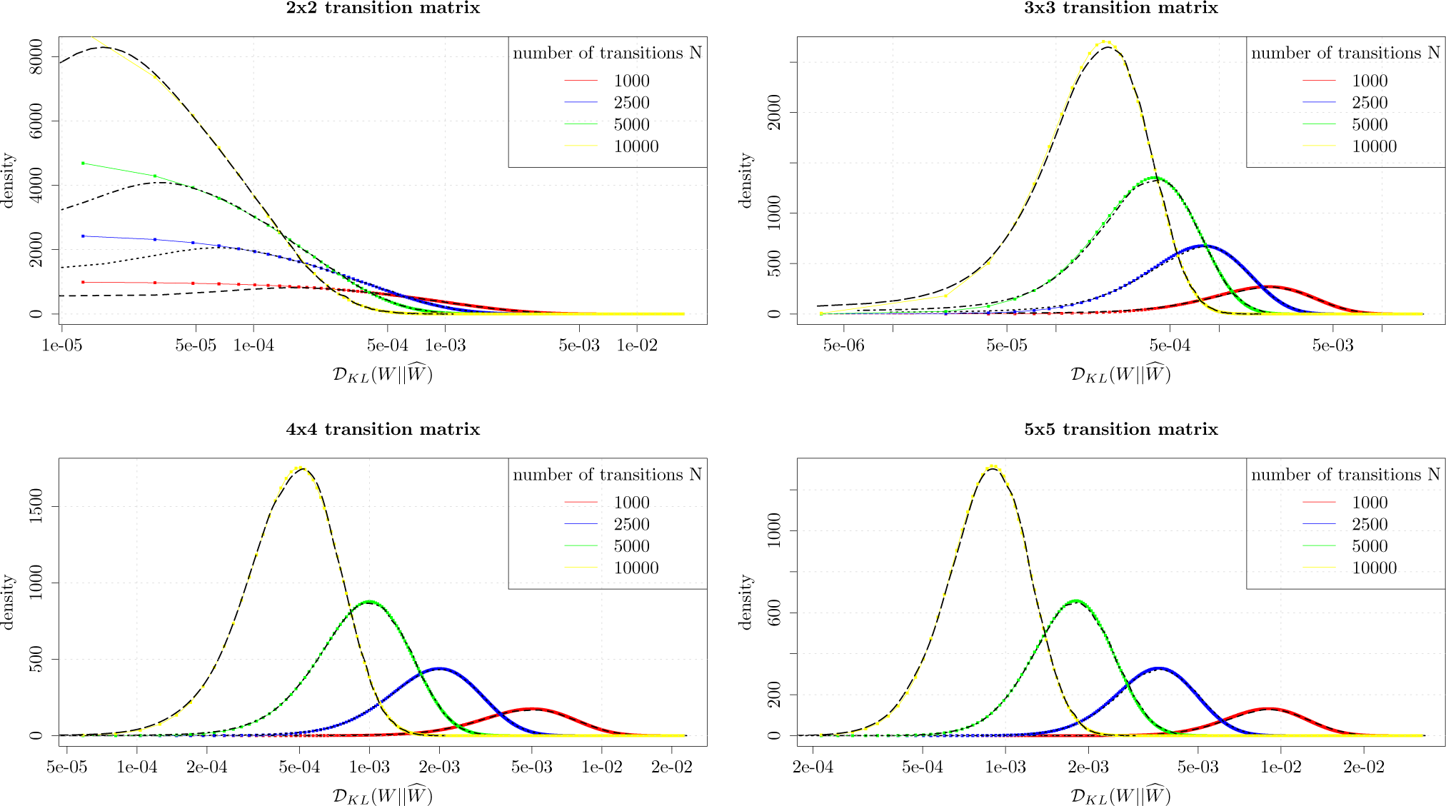
In order to evaluate the quality of the distributional approximation we have performed numerical simulations and compared the density of the approximate distribution in Equation (16) with density obtained through Monte Carlo simulations. We have generated densities of Kullback-Leibler divergence through Monte Carlo simulations for 2-by-2, 3-by-3, 4-by-4 and 5-by-5 transition probability matrices modeling first order Markov processes. The matrix W is selected in a random manner and we generate 50,000 realizations of ${\mathcal{D}}_{KL}(W\parallel \widehat{W})$, whereas Ŵ is obtained through sampling from the time series drawn from W, while N, the number of transitions, is set to 1000, 2500, 5000 and 10,000, respectively.

Figure 1 shows a good agreement between Monte Carlo simulations and approximation Equation (16). We conclude that Equation (16) is suitable for approximating Kullback-Leibler divergence distributions. We note that there is a slight divergence between the numerically simulated density and the approximation, for the 2-by-2 matrices.

3. Information Memory Loss

In this section, we present a novel method to evaluate memory within time series modeled as discrete Markov processes. First, we describe the procedure of Markov process extensions, whereas we extend the transition probabilities of Markov process to arbitrary high order. Applying the results presented in Section 2 on distributional properties of Kullback-Leibler divergence, we introduce an information theoretic measurement termed information memory loss that describes the memory content within time series modeled as discrete Markov process. We present the measurement on toy examples and on FX data during the unraveling of 2008 financial crisis.

We start by describing the procedure to compare Markov processes of different orders. Let W denote the transition probability matrix of order k

$$W=[\mathbb{P}((s_{i_k}\to \cdots \to s_{i_l}\to \cdots \to s_{i_1})\to s_1)]s_i,s_{i_1},\dots ,s_{i_k}\in \mathcal{S}$$

(18)

and let W′ denote the transition probability matrix of order l

$$W^{\prime }=[\mathbb{P}((s_{i_l}\to \cdots \to s_{i_1})\to s_1)]$$

(19)

Let us assume, without loss of generality that l < k. We extend the lower l-th order Markov process to a k-th order Markov process by assigning the new probabilities

$$\mathbb{Q}((s_{i_k}\to \cdots \to s_{i_l}\to \cdots \to s_{i_1})\to s_1)=\mathbb{P}((s_{i_l}\to \cdots \to s_{i_1})\to s_1).$$

(20)

In other words, we create an artificial k-th order Markov process prescribed by transitions probabilities $\mathbb{Q}((s_{i_k}\to \cdots \to s_{i_l}\to \cdots \to s_{i_1})\to s_1)$ whereas the transition probabilities are ignorant of the history beyond the l-th state, since they are set by transition probabilities of the l-th order Markov process. Therefore, if we denote with Ŵ the transition probability matrix of the extended k-th order Markov process, we obtained two matrices W and Ŵ, both of k-th order

$$W=[\mathbb{P}((s_{i_k}\to \cdots \to s_{i_l}\to \cdots \to s_{i_1})\to s_1)]$$

(21)

$$\widehat{W}=[\mathbb{Q}((s_{i_k}\to \cdots \to s_{i_l}\to \cdots \to s_{i_1})\to s_1)].$$

(22)

We refer to the mentioned procedure as Markov process extension and are set to compare matrices of Markov processes of different orders.

According to the results on distributional properties of Kullback-Leibler divergence presented in Section 2, viewing the transition probability matrix Ŵ as an estimate from a finite time series drawn from W, the Kullback-Leibler divergence ${\mathcal{D}}_{KL}(W\parallel \widehat{W})$ has the following approximate distribution (Equation (16)). We denote with ${\mathbb{F}}_{\mathrm{\Gamma }}$ the cumulative distribution function of sum of gamma distributed random variables with parameters $\frac{M_i(i-1)}{2}$ and $\frac{1}{N}$, i = 1, …, M and we call the percentile

$$Iml={\mathbb{F}}_{\mathrm{\Gamma }}{\mathcal{D}}_{KL}(W\parallel \widehat{W})$$

(23)

information memory loss. Hence, the Iml is an information theoretic measurement of memory embedded within the time series. Values close to 0 indicate the lower order Markov is suitable approximation for the higher order Markov process, as there is no loss of information using the lower order Markov process. On the other hand, values close to 1 indicate the lower order Markov process does not appropriately approximate the higher order Markov process, implying there is significant memory embedded within the process beyond what is modeled by the lower order Markov process.

The Iml provides us with a procedure to establish optimal order of Markov process. Given a sample time series, we estimate the transition probability matrix W of the (l + 1)-th order Markov process and we estimate transition probability matrix Ŵ of the l-th order Markov process. Then we compute Iml and for a pre-specified level of significance α ∈ [0, 1] we either accept or reject the hypothesis that there is no loss of information if we use a lower order process to approximate a higher order process. In other words, if Iml > 1 − α we reject the hypothesis that l-th order process adequately approximates an (l + 1)-th order process. We repeat this procedure for all l > 1, until we no longer reject the hypothesis for a pre-specified level of significance α and chose the last l as the optimal order of the Markov process.

We address the Iml measurement against three methods for determining the optimal order of Markov process: AIC [8], BIC [9] and χ² test [10]. AIC has had a fundamental impact in statistical model evaluation problems and has been applied to the problem of estimating the order of autoregressive processes and Markov processes. The estimator was derived as an asymptotic estimate of the Kullback-Leibler divergence. AIC is the most used and successful estimator of the optimal order of Markov process at the present time, as it performs better than BIC estimator for samples of relatively small size. Both AIC and BIC do not provide a test of a model in the sense of testing a null hypothesis, i.e., they can tell nothing about the quality of the model in an absolute sense—order selection is heuristic as the order estimator is usually defined as the minimizing value of this information criterion. χ² test can evaluate that a Markov process is of a given order against a larger order. In particular, with it we can test the hypothesis that a process has rth-order against (r + 1)th-order, until the test rejects the null hypothesis and then choose the last r as the optimal order. We note that as the χ² test relies on asymptotic distribution of χ² statistics, it does not take into account the sample size. On the other hand, the Iml is a theoretical information measurement that determines the optimal order of a Markov process in an absolute sense, i.e., it provides a statistical test, and it takes into account both the sample size and the number of estimated parameters.

To illustrate the measurement, we first present the Iml on a toy examples where we prescribe the order of a Markov process, and then evaluate the suitable order. We arbitrarily set the Markov process to be of fifth order, i.e., the history of previous five states impacts the transition probabilities to next possible states, while the transition probability matrix is set in a random manner. Equipped with this process, we then generate a time series of 1000 transitions, and estimate both W and Ŵ. For each pair of lower and higher order Markov processes we repeat the procedure 10,000 times and obtain the average Kullback-Leibler divergence and compute the Iml.

Table 1. The table presents the Iml and Kullback-Leibler divergence in brackets, for all possible combinations of higher and lower order Markov processes.

		W (Lower Order Markov Process)
		1st	2nd	3rd	4th	5th	6th
W higher order Markov process	2nd	0.99 (0.02)	–	–	–	–	–
	3rd	1.00 (0.07)	1.00 (0.28)	–	–	–	–
	4th	1.00 (0.11)	1.00 (0.31)	1.00 (0.30)	–	–	–
	5th	1.00 (0.17)	1.00 (0.34)	1.00 (0.32)	1.00 (0.14)	–	–
	6th	1.00 (0.16)	1.00 (0.32)	1.00 (0.30)	1.00 (0.14)	3.22 × 10−6(0.02)	–
	7th	0.99 (0.14)	1.00 (0.29)	1.00 (0.27)	0.98 (0.13)	7.87 × 10−22(0.02)	4.91 × 10−51(0.01)

reports Iml values, along with Kullback-Leibler divergence in brackets, for all possible combinations of lower and higher order Markov processes. As we can notice, the Iml correctly diagnoses suitable order of the Markov process—for all cases when the lower order is less than five, the measurement has a value of 1, indicating that the lower order process does not correctly approximate the higher order process, as there is memory embedded within the process that is not correctly modeled by a Markov process of order smaller than five. For the purpose of comparison to other methods, we have also used AIC, BIC and χ² test to determine the optimal order on the toy example. χ² test correctly identifies that the Markov process is of fifth order. On the other hand, both AIC and BIC do not correctly identify the optimal order of Markov process in all evaluated cases. For instance, both methods claim that the second order Markov process is the best approximation of the seventh order Markov process-false, as we have prescribed the Markov process to be of fifth order. We note that the mistake might be due to heuristic order selection criteria for AIC and BIC.

Second, we illustrate the dynamics of Iml within an empirical setting, on the AUD/JPY exchange rate during the unfolding of 2008 financial crisis. Financial time series returns exhibit fast decaying autocorrelation function[18] and nonlinearity [19], hence we find it suitable to model the price trajectory with low order Markov process and evaluate price trajectory with information theoretic measurements. If the dynamics of the financial time series rapidly changes, we try to capture it with a fourth order Markov process. We map the exchange rate price trajectory onto an 0.025% price grid, therefore the state space $\mathcal{S}$ consists of two states 0 and 1; 0 denotes a downward price move of 0.025% while 1 denotes an upward price move of 0.025%. Assigning the price grid in the mentioned manner assures that according to empirical scaling laws [23], on average we have a transition every 8 s. We chose a sliding window of one day, and with the transitions within the sliding window we estimate the transition probability matrix $W=[\mathbb{P}((s_{i_4}\to \cdots \to s_{i_1})\to s_i)]$ as a fourth order Markov process

$$\mathbb{P}((s_{i_4}\to \cdots \to s_{i_1})\to s_i)=\frac{n_{(s_{i_4}\to \cdots \to s_{i_1})\to s_i}}{n_{(s_{i_4}\to \cdots \to s_{i_1})\to \cdot }}$$

(24)

and another transition probability matrix W′ describing a first order Markov process estimated as

$$\mathbb{P}(s_{i_1}\to s_i)=\frac{n_{s_{i_1}\to s_i}}{n_{s_{i_1}\to \cdot }}$$

(25)

where $n_{(s_{i_4}\to \cdots \to s_{i_1})\to s_i}$ and $n_{s_{i_1}\to s_i}$ denotes the number of transitions within a sliding time window of one day with dynamics $(s_{i_4}\to \cdots \to s_{i_1})\to s_i$ and $(s_{i_1}\to s_i)$, respectively and

$$\begin{array}{c}{n}_{(s_{i_4}\to \cdots \to s_{i_1})\to \cdot }={\displaystyle \sum _{s\in \mathcal{S}}{n}_{(s_{i_4}\to \cdots \to s_{i_1})\to s}}\\ n_{s_{i_1}\to \cdot }={\displaystyle \sum _{s\in \mathcal{S}}{n}_{s_{i_1}\to s\cdot }}a\end{array}$$

In other words, the matrix W contains the memory of price trajectory from the four previous states, while the matrix W′ contains the memory only of the current state. We then extend the lower, first order Markov process as described in Equation (20) and compute the Kullback-Leibler divergence to obtain the Iml. The sliding window is moved forward by one hour, each time obtaining transitions for estimation procedure described above.

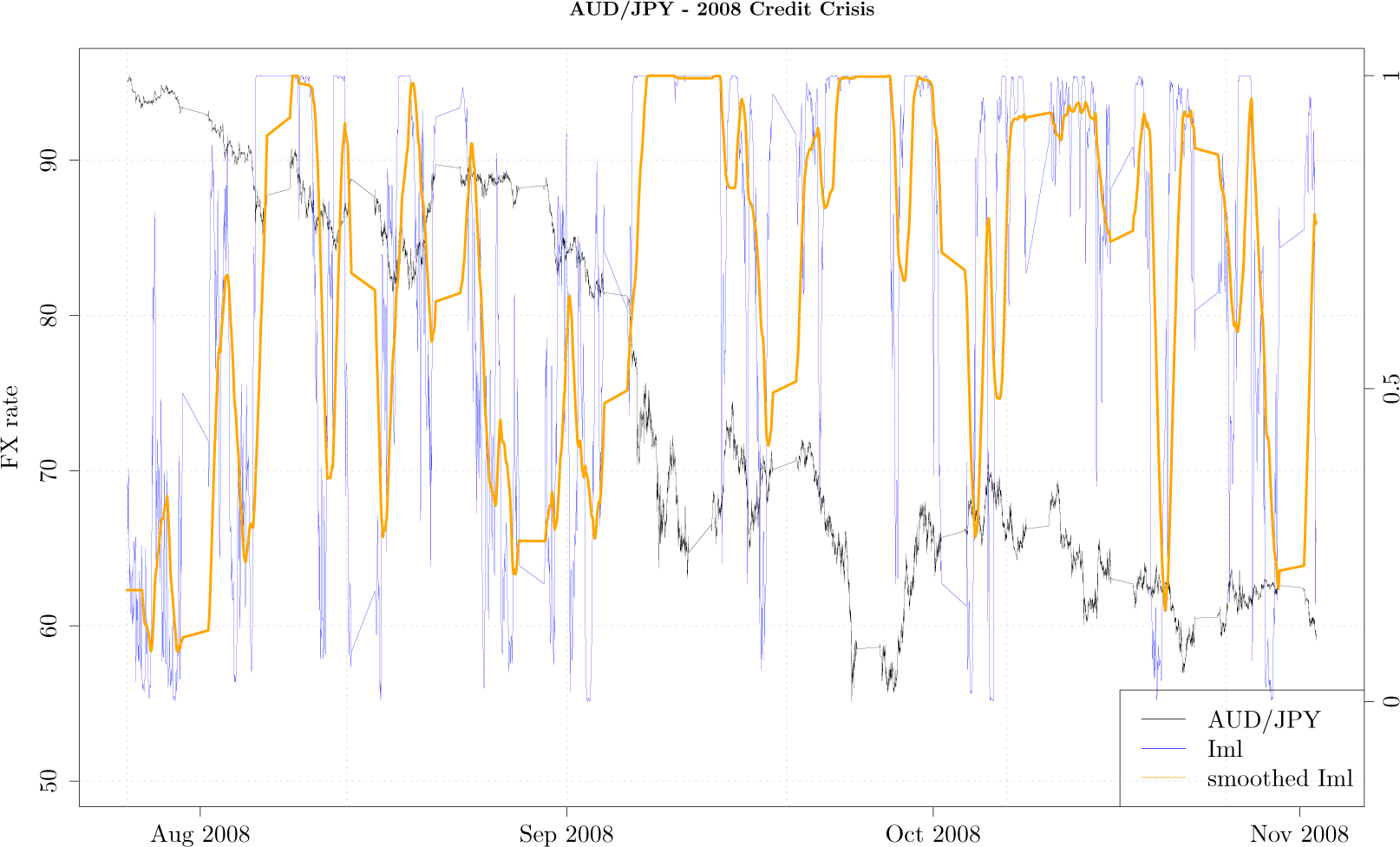
Figure 2 shows the tick-by-tick AUD/JPY exchange rate (black curve) during the period from August 2008 till end of November 2008, along with the Iml (blue curve) and Iml smoothed with 20 point moving average (orange curve). While during the month of August 2008 as the exchange rate was slowly moving lower, the measurement gently oscillated around values close to zero, indicating the AUD/JPY exchange rate exhibits usual property of fast decaying autocorrelation. The rapid decline in the exchange rate of almost 30% corresponds to the month of September 2008 when the measurement has a value close to 1, indicating that the lower order Markov process is not a good approximation of the higher order Markov process. In other words, over this dramatic period the price movement as mapped onto a fixed grid exhibits memory beyond the first order Markov process. This is intuitive as the sharp downward movement of the FX rate, when autocorrelation drastically increases, cannot be captured by low order Markov processes. As it turns out, during the month of September 2008 many financial markets around the world crashed as Lehman Brothers filed for bankruptcy, and our measurement seems to be able to capture this unusual activity.

4. Information Codependence Structure

In this section we present a novel method to evaluate co-dependence among times series modeled as Markov processes. We construct a transition probability matrix that assumes no co-dependence among the transitions of Markov processes, and applying the results presented in Section 2 on distributional properties of Kullback-Leibler divergence we introduce an information theoretic measurement that indicates the co-dependence structure among Markov processes. We illustrate the application of the measurement on a toy example and on EUR/USD and USD/CHF exchange rates during 2010/2011 Euro crisis, when USD/CHF weakened almost 20% in one month.

We start by presenting how to create a process comprised of Markov processes, a joint Markov process. Let us assume we have m Markov processes with states denoted as s_i ∈ ${\mathcal{S}}_i$ and let W_i, i = 1, …, m denote the accompanying transition probability matrices. We construct the states s ∈ ${\mathcal{S}}_1\times \cdots \times {\mathcal{S}}_m$ of joint Markov process in the following manner

$$s=({\mathrm{s}}_1,\dots ,s_m)\in {\mathcal{S}}_1\times \cdots \times {\mathcal{S}}_m$$

(26)

Therefore, the transition probability matrix of a joint Markov process is denoted with W

$$W=[\mathbb{P}({\mathrm{s}}^{\prime }\to {\mathrm{s}}^{″})]{\mathrm{s}}^{\prime },{\mathrm{s}}^{″}\in {\mathcal{S}}_1\times \cdots \times {\mathcal{S}}_m$$

(27)

We assume that when a transition occurs on the joint Markov process, it is a manifest of transition on some i-th Markov process. In other words, only one Markov process can experience a transition at any given moment.

We now present the construction of the structureless transition probability matrix that assumes no co-dependence structure among the transitions of Markov processes comprising the joint Markov process. For simplicity, we present the derivation when the transitions are modeled as a first order Markov processes, stressing the procedure is the same in case the transitions are modeled as higher order Markov processes.

Let ${\mathrm{s}}^{\prime }=(s_1^{\prime }\dots ,s_m^{\prime })$, $s^{″}=(s_1^{″}\dots ,s_m^{″})$ ∈ ${\mathcal{S}}_1\times \cdots \times {\mathcal{S}}_m$ and we observe the following transition probability

$$\mathbb{P}({\mathrm{s}}^{\prime }\to {\mathrm{s}}^{″})$$

(28)

The underlying dynamics of transitions on the joint Markov process implies that the transition occurs on some i-th Markov process, therefore the probability in Equation (28) equals

$$\mathbb{P}({\mathrm{s}}^{\prime }\to {\mathrm{s}}^{″})=\mathbb{P}(\{{\mathrm{s}}^{\prime }\to {\mathrm{s}}^{″}\}\cap \left\{i\text{-th markov process transitioned}\right\})$$

(29)

$$\mathbb{P}({\mathrm{s}}^{\prime }\to {\mathrm{s}}^{″})=\mathbb{P}(\{{\mathrm{s}}^{\prime }\to {\mathrm{s}}^{″}\}|i\text{-th markov process transitioned})\mathbb{P}(i\text{-th markov process transitioned})$$

(30)

In case there is no dependence among the Markov process the resulting probability equals

$${\mathbb{P}}_i(s_i^{\prime }\to s_i^{″})\mathbb{P}(i\text{-th markov process transitioned})$$

(31)

where the probability ${\mathbb{P}}_i(s_i^{\prime }\to s_i^{″})$ is obtained from W_i of i-th Markov process, since independence implies that the transitions in i-th Markov process does not depend on states on other Markov processes.

We need to obtain the probability ℙ (i-th Markov process transitioned); we denote with $s_i^{(1)},\dots ,s_i^{(k_i)}$ the possible transitions from state $s_i^{\prime }$ (with $s_i^{″}$ being one of them) and let $N(s_i^{\prime }\to s_i^{(j)})$ denote the number of transitions in the sample from $s_i^{\prime }$ to $s_i^{(j)}$. Therefore, the aforementioned probability equals

$$\mathbb{P}(i\text{-th markov process transitioned})=\frac{{\displaystyle {\sum }_{j=1}^{k_i}N(s_i^{\prime }\to s_i^{(j)})}}{{\displaystyle {\sum }_{l=1}^m{\displaystyle {\sum }_{j=1}^{k_i}N(s_l^{\prime }\to s_l^{(j)})}}}$$

(32)

We denote the structureless transition probability matrix with W₁⊕…⊕W_m and set the transition probabilities to

$$W_1\underset{¯}{\oplus }\dots \underset{¯}{\oplus }{W}_m=[{\mathbb{P}}_i(s_i^{\prime }\to s_i^{″})\mathbb{P}(i\text{-th markov process transitioned})]s_i^{\prime },s_i^{″}\in {\mathcal{S}}_i,i=1,\dots ,m$$

(33)

Hence the matrix W₁⊕…⊕W_m models the transitions of a joint Markov process assuming there is no co-dependence structure among Markov processes i = 1, …, m.

We denote with ${\mathbb{F}}_{\mathrm{\Gamma }}$ the cumulative distribution function of Kullback-Leibler divergence distribution presented in Equation (16). We call the percentile

$$Ics={\mathbb{F}}_{\mathrm{\Gamma }}({\mathcal{D}}_{KL}(W\parallel W_1\underset{¯}{\oplus }\dots \underset{¯}{\oplus }{W}_m))$$

(34)

information codependence structure that provides information theoretic measurement of co-dependence among Markov processes i = 1, …, m comprising the joint Markov process.

In order to validate the Ics as a method to evaluate the co-dependence among Markov processes, we test it on a toy example where two Markov processes are Brownian motions linked by a correlation coefficient ρ

$$d{S}_t^i=\sigma d{W}_t^i,i=1,2$$

(35)

$$\langle d{W}_t^1,d{W}_t^2\rangle \rho$$

(36)

where the volatility σ is set to 25% and we vary ρ along an equidistant grid, from −1.0 to 1.0 with a step of 0.01, obtaining a total of 201 values. We map the price movement of both time series onto a fixed grid of 0.1%, where 1 denotes an upward move of 0.1% while 0 denotes a downward move of 0.1%. Therefore, both Markov processes have the state space $S_i=\left\{0,1\right\}$, i = 1, 2 and we can create the joint Markov process with state space ${\mathcal{S}}_1\times {\mathcal{S}}_2={\left\{0,1\right\}}^2$. We generate 1500 transitions for the joint Markov process, estimate the joint transition probability matrix W, construct the structureless transition probability matrix W₁⊕W₂ and compute the Kullback-Leibler divergence ${\mathcal{D}}_{KL}(W\parallel W_1\underset{¯}{\oplus }{W}_2)$. We repeat this procedure 10,000 times and obtain the average Kullback-Leibler divergence, finally computing Ics.

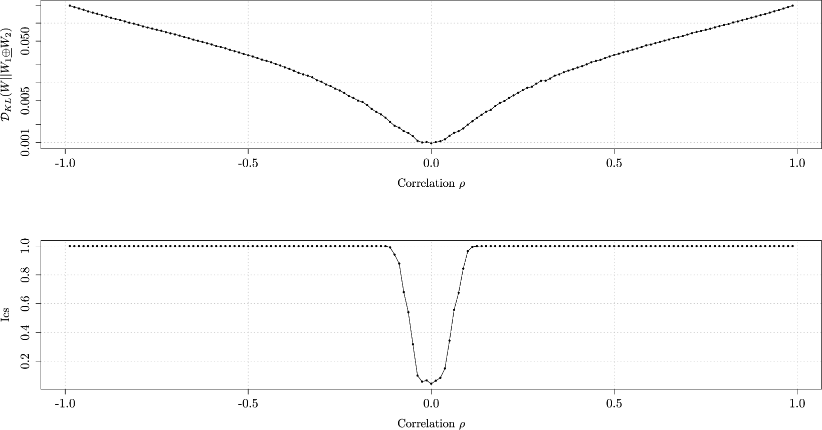
Figure 3 graphs the average Kullback-Leibler divergence and the Ics as a function of correlation coefficients ρ. We notice that for values of ρ smaller than −0.10 and larger than 0.10, the measurement correctly identifies the Markov processes are in fact not independent as the Ics has a value of 1. For the values of correlation within interval [−0.10, 0.10] the measurement is not able to identify co-dependence. As we would increase the number of transitions, the procedure would be able to identify co-dependence for values of correlation within [−0.10, 0.10].

We illustrate the dynamics of the Ics on the EUR/USD and USD/CHF exchange rates during the unfolding of 2010/2011 Euro Crisis, when USD/CHF weakened almost 20% in one month. The codependence between financial time series returns exhibits Epps effect, the phenomenon that the empirical correlation decreases as sampling frequency increases [20]. The phenomenon is caused by asynchronous trading, nonlinearity, discretisation and herding behavior [21,22]. Therefore, we find the event based framework and information theoretic measurement suitable for capturing codependence among financial time series. We map both exchange rate price trajectories onto an 0.025% price grid: downward move of 0.025% is denoted with 0, while an upward move of 0.025% is denoted with 1. Assigning such a price grid assures that according to empirical scaling laws [23], on average the transitions on the joint Markov process occur approximately every 4 seconds. The Markov process, both for EUR/USD and USD/CHF exchange rate have the state space $S_i=\left\{0,1\right\}$, i = 1, 2 and we create the joint Markov process with state space ${\mathcal{S}}_1\times {\mathcal{S}}_2={\left\{0,1\right\}}^2$. We arbitrary model the transitions on both the joint Markov process and Markov processes i = 1, 2 describing the transitions on individual exchange rates as third order processes

$$W=\left[\mathbb{P}\right(({\mathrm{s}}_4\to {\mathrm{s}}_3\to {\mathrm{s}}_2)\to {\mathrm{s}}_1)]$$

(37)

$$W_i=[\mathbb{P}{((s}_i^4\to {\mathrm{s}}_i^3\to {\mathrm{s}}_i^2)\to {\mathrm{s}}_i^1)],i=1,2$$

(38)

We choose the sliding time window for transitions to equal one day and use the transitions within the sliding window to estimate the transition probabilities

$$\mathbb{P}(({\mathrm{s}}_4\to {\mathrm{s}}_3\to {\mathrm{s}}_2)\to {\mathrm{s}}_1)=\frac{n_{{(s}_4\to {\mathrm{s}}_3\to {\mathrm{s}}_2)\to {\mathrm{s}}_1}}{n_{{(s}_4\to {\mathrm{s}}_3\to {\mathrm{s}}_2)\to \cdot }}$$

(39)

$$\mathbb{P}{((s}_i^4\to {\mathrm{s}}_i^3\to {\mathrm{s}}_i^2)\to {\mathrm{s}}_i^1)=\frac{n_{{(s}_i^4\to {\mathrm{s}}_i^3\to {\mathrm{s}}_i^2)\to {\mathrm{s}}_i^1}}{n_{{(s}_i^4\to {\mathrm{s}}_i^3\to {\mathrm{s}}_i^2)\to \cdot }},i=1,2$$

(40)

where $n_{({\mathrm{s}}_4\to {\mathrm{s}}_3\to {\mathrm{s}}_2)\to {\mathrm{s}}_1}$ denotes the number of transitions within the sliding time window on the joint Markov process with dynamics $({\mathrm{s}}_4\to {\mathrm{s}}_3\to {\mathrm{s}}_2)\to {\mathrm{s}}_1$, and $n_{{(\mathrm{s}}_i^4\to {\mathrm{s}}_i^3\to {\mathrm{s}}_i^2)\to {\mathrm{s}}_i^1}$ denote the number of transitions the sliding time window on i-th Markov process with dynamics ${(s}_i^4\to {\mathrm{s}}_i^3\to {\mathrm{s}}_i^2)\to {\mathrm{s}}_i^1$, i = 1, 2 and

$$n_{{(\mathrm{s}}_4\to {\mathrm{s}}_3\to {\mathrm{s}}_2)\to \cdot }={\displaystyle \sum _{\mathrm{s}\in {\mathrm{S}}_1\times {\mathrm{S}}_2}{n}_{{(\mathrm{s}}_4\to {\mathrm{s}}_3\to {\mathrm{s}}_2)\to \mathrm{s}}}$$

(41)

$$n_{{(\mathrm{s}}_i^4\to {\mathrm{s}}_i^3\to {\mathrm{s}}_i^2)\to \cdot }={\displaystyle \sum _{\mathrm{s}\in {\mathcal{S}}_i}{n}_{{(\mathrm{s}}_i^4\to {\mathrm{s}}_i^3\to {\mathrm{s}}_i^2)\to s},i=1,2}$$

(42)

The sliding window is moved forward by one hour, each time obtaining transitions for estimation procedure described above. We construct the structureless transition probability matrix W₁⊕W₂ as described above, compute the Kullback-Leibler divergence ${\mathcal{D}}_{KL}(W\parallel W_1\underset{¯}{\oplus }{W}_2)$ and obtaining the Ics.

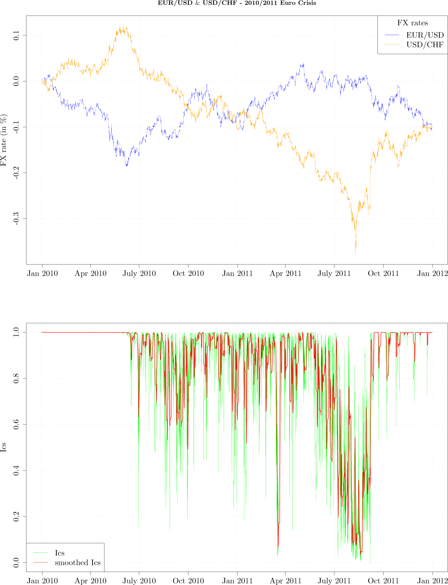
In Figure 4, the upper graph shows tick-by-tick EUR/USD (blue curve) and USD/CHF (orange curve) exchange rates during the period from January 2010 till January 2012. In the lower graph the green curve graphs hourly Ics, while the red curve graphs hourly Ics smoothed with a 20 point moving average. For the first six months of year 2010 the measurement Ics had a value of 1 indicating the exchange rate movements as mapped onto a fixed grid are not independent; this is intuitive as the exchange rates during that period look as mirror images of each other. In other words, the exchange rates were strongly codependent. For the period of next twelve months the measurement experiences periods that indicate the co-dependence is breaking apart, which finally culminated in the month of July 2011, as the USD/CHF exchange rate weakened by almost 20%. During the mentioned period Figure 4 shows that the exchange rates ceased to look as mirror images of each other—the USD/CHF exchange rate started its depreciation and there are several moments when Ics briefly dropped indicating the codependence is weakening. It is easy to notice from the upper graph that from July till October 2011 the exchange rates codependence broke apart as the USD/CHF significantly weakened, while the EUR/USD moved in a narrow range. The Swiss National Bank intervened in the FX market on 6 September 2011 to stop the strengthening of the Swiss Franc, at which point the exchange rate codependence re-emerged and the Ics achieved again a value of 1. We have also computed correlation and mutual information on 5 min logarithmic returns, with a sliding window of one day, noticing both measurement oscillate a lot more than Ics, even during period from January 2010 till July 2010, when it is clear EUR/USD and USD/CHF exhibit strong negative codependence.

5. Conclusions

We have presented novel information theoretic based methods to determine the optimal order as well as co-dependence relationships between Markov processes. To establish the new measurements, we have derived an approximate for the distribution of Kullback-Leibler divergences between an known transition probability matrix and its sample estimate, as a sum of gamma distributed random variables that has been validated with Monte-Carlo simulations. We have tested the validity of both measurements by considering toy examples as well as empirical financial data.