Oxygen Saturation and RR Intervals Feature Selection for Sleep Apnea Detection

Abstract

A diagnostic system for sleep apnea based on oxygen saturation and RR intervals obtained from the EKG (electrocardiogram) is proposed with the goal to detect and quantify minute long segments of sleep with breathing pauses. We measured the discriminative capacity of combinations of features obtained from RR series and oximetry to evaluate improvements of the performance compared to oximetry-based features alone. Time and frequency domain variables derived from oxygen saturation (SpO2) as well as linear and non-linear variables describing the RR series have been explored in recordings from 70 patients with suspected sleep apnea. We applied forward feature selection in order to select a minimal set of variables that are able to locate patterns indicating respiratory pauses. Linear discriminant analysis (LDA) was used to classify the presence of apnea during specific segments. The system will finally provide a global score indicating the presence of clinically significant apnea integrating the segment based apnea detection. LDA results in an accuracy of 87%; sensitivity of 76% and specificity of 91% (AUC = 0.90) with a global classification of 97% when only oxygen saturation is used. In case of additionally including features from the RR series; the system performance improves to an accuracy of 87%; sensitivity of 73% and specificity of 92% (AUC = 0.92), with a global classification rate of 100%.

1. Introduction

Obstructive Sleep Apnea (OSA) is a disorder characterized by intermittent cessation of breathing due to upper airway closure during sleep. If breathing ceases completely, the event is called apnea. In case that it does not completely cease, but there is a marked reduction of air entering the lungs, the event is called hypopnea [1].

As a consequence of OSA there is also an increase in arousals and fragmentation of the sleep [2]. Development of concomittent morbidities such as cardiovascular problems, for example complex tachyarrhythmias including atrial fibrillation, and symptoms such as daytime somnolence, cognitive impairment and mood changes may decrease life expectancy and affect quality of life making of OSA a serious disease. OSA is highly prevalent and represents a significant area of clinical respiratory practice in developed countries [3].

The American Academy of Sleep Medicine (AASM) Manual specifies details for the recording and scoring of sleep and associated events in a sleep center [4]. It is used to score the breathing events. Overnight polysomnography (PSG), is the accepted diagnostic tool for sleep apnea [4–6]. Apnea severity is quantified by calculating the apnea-hypopnea index (AHI) which is the number of apnea and hypopnea events per hour of sleep. Performing PSGs is a costly [7] and labor-intensive technique that is not only uncomfortable for the patient but also not available in all areas [8], leading to the need to develop new diagnostic strategies to enable ambulatory diagnoses and thus reduce the demand of PSGs.

A decrease in the oximetry levels may be secondary to hypoventilation and it is also dependent on the oxyhemoglobin desaturation dynamic. So, oximetry is considered a surrogate indirect method for sleep apnea screening [9]. Repetitive oxygen desaturations are highly specific to apnea. However, the sensitivity of oximetry with such criterion is generally low because it is not unusual for patients to display normal oximetry during apnea events if they are short. It is also possible that some desaturations are not the result of breathing pauses but may be caused by chronic obstructive pulmonary disease (COPD) [10] or alveolar hypoventilation. We additionally, in the hope to improve on those results, explore a large number of linear and non linear variables describing features of the heart rate variability (HRV) [11,12] that are extracted from the RR intervals in order to evaluate their performance and compare the results if combined with oximetry.

In this work we apply forward feature selection in order to improve the performance of apnea screening and find variables which describe patterns in presence of OSA with more detail. Linear Discriminant Analysis (LDA) is being proposed in order to decide on the presence of apnea in segments of one minute length. The system will finally provide a global score indicating the presence of clinically significant apnea integrating the segment based apnea detection.

2. Materials and Methods

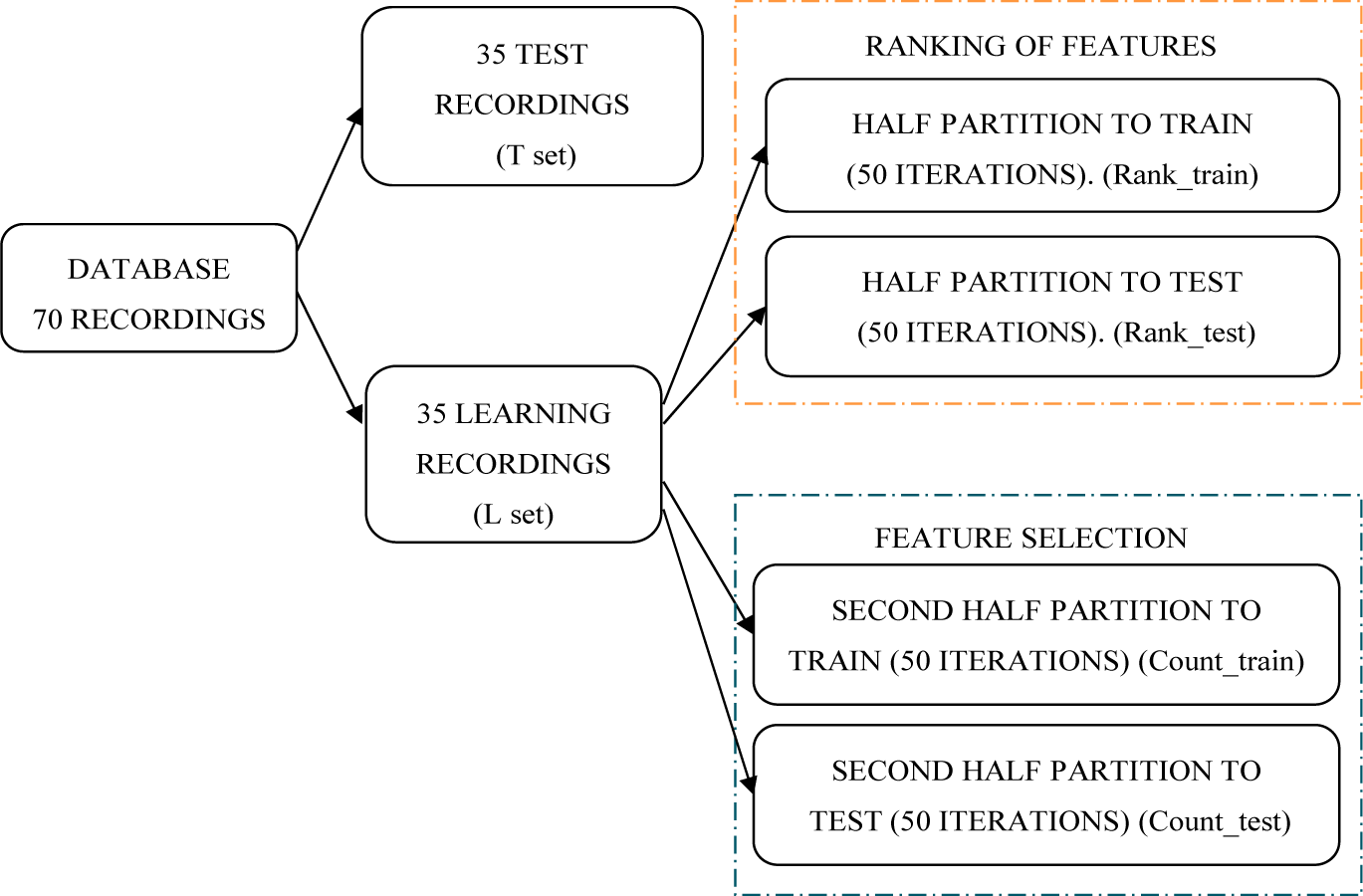
2.1. Data Sets

The database was provided by the Sleep Unit of the Dr. Negrín Gran Canaria University Hospital. It contains recordings of 70 patients (51 males and 19 females, 18 to 82 years old) that were referred to the sleep clinic because of suspected OSA. Patients did not suffer from heart diseases. Arrhythmic subjects were excluded from the study. Total sleep time was at least 3 h. Comorbid nonrespiratory sleep disorders were not suspected at the time of referral to polysomnography, even though no protocol to exclude certain disorders (e.g., insomnia) was used. Some patients referred to polysomnography are found to be snorers without clinical relevant sleep apnea (AHI < 5). All patients were examined by one of two experts in sleep medicine.

The used recordings contain a single electrocardiogram (EKG) digitized at 200 Hz with 16-bit resolution and oxygen saturation (SpO2) signals with 50 Hz sampling rate and 16 bits resolution. Individual recordings vary in length from slightly less than 230 min to 486 min. Recordings were collected using a computerized system from VIASYS Healthcare Inc. (Wilmington, MA, USA). The sleep studies were scored for respiratory events according to the AASM criterion [4].

The manual detection of respiratory events was performed for every 30 s interval according to standard AASM criterion and an apnea hypopnea index (AHI), indicating the number of events per hour of sleep, was calculated according to the PSG analysis. The respiratory annotations were mapped to segments of one minute length indicating the presence or absence of apnea or hypopnea during that minute. This segment length was chosen to correspond to the one chosen in the Computers in Cardiology Challenge 2000 [13] to allow for better comparability. Minutes were annotated as either normal breathing or disturbed breathing.

The records have been divided into a group of learning data (L set) and a group of test data (T set) of equal size. Each group consists of 35 EKG recordings. L set contains 15,170 1-minute training epochs and T set, 14,373 epochs. We considered an AHI threshold of 10 to differentiate between control and apnea group. This is based on the criterion as used in the CinC Challenge 2000. We define three classes: class A (apnea), class B (borderline) and class C (control). Below we define each class:

• Class A (46 recordings): Recordings contain AHI greater than or equal to 10 and at least 70 min with apnea. Both the L set and the T set contain 23 recordings fitting this criterion.
• Class B (4 recordings): Recordings contain AHI greater or equal to 5 and between 5 and 69 min with apnea. There are two recordings in each group (L and T set) that fit this criterion.
• Class C (20 recordings): These recordings can be considered normal since AHI is lower than 5. Both groups (L and T set) contain 10 recordings of class C.

For the use in this paper we have combined Groups A and B to present as a single “apnea” group. Since the used dataset does not contain any recording of an AHI > 5 but < 10 the difference between A and B mostly reduces to differences in sleeping time which does not add to the analysis. The data of the polysomnography is presented in

Table 1. Description of polysomnography data for different groups in the database: AHI, dips/h (desaturations events per hour) and apnea hypopnea duration in seconds. Results are represented as mean (min-max).

SUBJECTS	AHI	DIPS/h	APNEA-HYPOPNEA DURATION (s)
APNEA (Group A and B)	48.87 (11–151.9)	53.65 (7.9–122.3)	17.8 (10–125)
NORMAL (Group C)	1.87 (0–4.8)	1.55 (0–4.3)	12 (0–30)

.

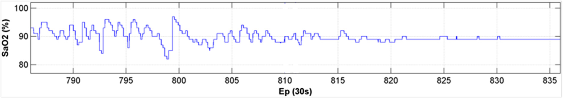
2.2. Time Domain Oximetry Features

During respiratory pauses in sleep, the oxygen saturation signal undergoes marked changes, making the variance of the signal a variable with high discriminatory power. To maximize the utility of this variable, the length of the segments has to be decided. According to the AASM [4] the minimum period necessary to consider a respiratory pause an apnea or hypopnea is 10 s. Some such events can be longer than 50 s; therefore, in this study, the variance will be considered for one minute segments, enabling the detection of both long and short apnea and hypopnea events. While it may be possible for more than one respiratory event to occur per minute interval, we will not consider this further. We will consider the variance in 1 and 5 min centered on a specific segment, called var Sat_1m and var Sat_5m respectively with one minute of displacement between adjacent frames, achieving a minute-by-minute analysis.

2.3. Frequency Domain Oximetry Features

A characteristic pattern of severe apnea is a cyclical drop in the levels of SpO₂, which, through spectral analysis, is possible to locate as a specific low-frequency component. The graph in Figure 1 shows exemplary the dynamic of an oximetry signal for 50 epochs of 30 s each in presence of apnea where it is possible to find oscillations between epoch 785 and 820.

The causal relationship between interruption in airflow and oxygen desaturation allows us to extract associated features from 5 min oximetry segments, with one minute of displacement between adjacent frames. The power spectrum of a SpO2 signal can be obtained through the periodogram with the following expression:

$$S\left(k\right)={\left|\frac{1}{N}{\displaystyle \sum _{n=0}^{N-1}\mathit{Sat}(n)e^{-j2\pi k/N}}\right|}^2$$

(1)

In order to extract features for different frequency bands the use of a filter bank is proposed. There are many ways to implement filter banks. One which may be considered having good computational properties is to develop a filter directly on the transformed domain [14]:

$$Y^{\prime }\left(m\right)=\frac{{\displaystyle \sum _{k=b_m-{\mathrm{\Delta }}_m}^{b_m+{\mathrm{\Delta }}_m}S(k)U_{{\mathrm{\Delta }}_m}(k)}}{{\displaystyle \sum _{k=0}^{\frac{N}{2}-1}S(k)}}1\le m\le M$$

(2)

A windowing process U is applied where Δ_m represents the bandwidth of the m^th filter and b_m the center frequency of the m^th band on the outcome of the periodogram calculated according to the expression (1). Total power term in the denominator appears to normalize the expression, N expresses the number of samples of S(k) and M is the number of output elements of the filter bank. In our particular case we use a bank of equally spaced 10 filters (M = 10).

2.4. Generation and Postprocessing of RR Intervals

The EKG is divided into five minutes segments with one minute of displacement between adjacent frames, achieving a minute-by-minute quantification. The central minute determines the index of said quantification. Then, the EKG is band pass filtered between 40 and 70 Hz, and the signal is full wave rectified and low pass filtered to 25 Hz.

An interval of values is set around a relative maximum of the output signal, locating the R peak as the maximum value of the EKG signal within that range. The time separation between successive R peaks provides the RR intervals. The use of RR intervals often requires the exclusion of misdetection due to artifacts as well additional ectopic values (e.g., premature ventricular complexes). An adaptive filtering procedure for automatic artifact removal, including ectopic beats, is applied [11]. The advantage of this algorithm is the spontaneous adaptation of the filter coefficients due to sudden changes in the RR intervals.

2.5. Time Domain RR Interval Features

A tachogram shows the temporal development of the heart rate as the interval duration of the RR or NN interval for either registered time or interval number (N is the set of normal RR intervals, eliminating artifacts and ectopic beats). This temporal development is also known as HRV that, while being able to be measured non-invasively, allows inferences regarding the activities of its main drivers the sympathetic and parasympathetic nervous systems. During sleep it is dominated by vagal efferent activity and from respiratory induced changes such in the venous return related mechanical sinus node stretch [15]. It has been shown that OSA is associated with autonomic imbalances and consequently changes in the HRV [16]. From the time domain, the following variables [12] have been calculated:

-

meanNN: the mean value of the NN-intervals in 5 min segments

-

sdNN: standard deviation of the NN-intervals in 5 min segments

-

cvNN: coefficient of variation of the NN-intervals (quotient of standard deviation and mean value of the filtered tachogram)

$$cvN{N}_{5m}=\frac{sdN{N}_{5m}}{meanN{N}_{5m}}$$

(3)

-

Rmssd: root mean square of successive 5 min of NN intervals:

$$Rmssd=\sqrt{\left(\frac{1}{N}{\displaystyle \sum _{n=1}^{N}N{N}^2{}_{5m}(n)}\right)}$$

(4)

-

sdaNN1: standard deviation of mean values of successive 1 min of NN-intervals:

$$sdaNN1={\left(\frac{{\displaystyle \sum _{n=1}^M{\left(meanN{N}_{1m}(n)-\frac{1}{M}{\displaystyle \sum _{n=1}^{M}meanN{N}_{1m}(n)}\right)}^2}}{M-1}\right)}^{1/2}$$

(5)

where M = 5, $meanN{N}_{1m}=\frac{1}{N}{\displaystyle \sum _{n=1}^{N}N{N}_{1m}(n)}$ and N is the number of NN intervals in a one minute segment.

The differences between successive NN intervals can provide information about vagal activity and is contained in group of variables pNNx [17,18]. Below is the list of specific instances of these variables calculated over 5 minute intervals:

-

pNN20: Percentage of NN-interval differences greater than 20 ms

-

pNN30: Percentage of NN-interval differences greater than 30 ms

-

pNN50: Percentage of NN-interval differences greater than 50 ms

-

pNN100: Percentage of NN-interval differences greater than 100 ms

-

pNN120: Percentage of NN-interval differences greater than 120 ms

-

pNN150: Percentage of NN-interval differences greater than 150 ms

Entropy is conceived of as a measure of disorder, uncertainty or information that can be gained by observation of disordered systems. Claude Shannon formally defined entropy as follows:

$$H=-{\displaystyle \sum _{i=1}^{n}p(i)\cdot \ln \mathrm{p}(\mathrm{i})}$$

(6)

where p(i) is the probability of the occurrence of a specific event.

Renyi entropy was introduced as a generalization of the Shannon entropy and is defined as follows:

$$H^{(\mathrm{q})}=\frac{1}{1-q}\ln \left({\displaystyle \sum _{i=1}^{n}p{(i)}^{(\mathrm{q})}}\right)$$

(7)

where q is a parameter which is greater than zero and different to one. The order q can be adjusted to make it more or less sensitive to the shape of the probability distributions. Renyi is generalized entropy where in the limit q →1, the Renyi entropy converges to the Shannon entropy.

We will use an estimate of the differential entropy for the observed RR intervals, using the probability density function estimated from histogram.

-

Shanon: The Shannon entropy in each 5 min tachogram is calculated by the following expression:

$$H=-{\displaystyle \sum _{i=1}^{n}f(x_i)\cdot \ln \left(\frac{f(x_i)}{\mathrm{w}\left(x_i\right)}\right)}$$

(8)

where f is the probability density function estimated from histogram obtained in each 5 min tachogram frame and w is the width of the i^th bin. In our particular case, the width of each bin is 20 ms leading to the total of n = 100 bins.

-

Renyi: Renyi entropy for a histogram of each 5 min tachogram is calculated. Expression (9) estimates the Renyi entropy:

$$H=\frac{1}{1-q}{{\displaystyle \sum _{i=1}^n\ln \left(\frac{f(x_i)}{\mathrm{w}(x_i)}\right)}}^q$$

(9)

where w is the width of the i^th bin. Entropies of order 2, 4 and 0.25 (Renyi2, Renyi4 and Renyi0.25) will be used.

-

noNNtime: Total time with artifacts in milliseconds.

2.6. Frequency Domain RR Interval Features

In order to obtain good frequency resolution, five minute EKG frames with a displacement of one minute between frames, will be considered [19,20].

As suggested in [21], in our work, the power spectral analysis of the RR series is performed by means of the periodogram method $R(k)={\left|\frac{1}{N}{\displaystyle \sum _{n=0}^{N-1}RR(n)e^{-j2\pi k/N}}\right|}^2$, which is a good tool to identify the dominant frequencies and their strength. We consider the estimated power following the task force recommendations [22], in the bands of interest detailed below:

-

ULF: power in the frequency band from 0 Hz up to 0.0033 Hz.

-

VLF: power in the frequency band from 0.0033 Hz up to 0.04 Hz.

-

LF: power in the frequency band from 0.04 Hz up to 0.15 Hz.

-

HF power in the frequency band from 0.15 Hz up to 0.4 Hz.

On the other hand, the following common used ratios have been used and were added to the previous variables:

-

LF/HF: ratio of LF and HF.

-

LF/P: ratio between LF and total power P.

-

HF/P: ratio of HF and total power P.

-

VLF/P: ratio between VLF and total power P.

-

ULF/P: ratio between ULF and total power P.

-

(ULF + VLF)/P: ratio of ULF + VLF and total power P.

-

(ULF + VLF + LF)/P: ratio of ULF + VLF + LF and total power P.

-

LFn: LF in normalized units, LF/(P − VLF) × 100.

-

HFn: HF in normalized units, HF/(P − VLF) × 100.

2.7. Measures of Non-linear Dynamics of RR Intervals

Some processes in autonomic regulation can be described reliably by linear methods. However the complexity in the modulation of the sinus node activity indicates the inclusion non-linear features. Applying non-linear dynamic methods gives additional information about the state of the cardiovascular and the autonomous nervous systems, especially for non-stationary parts of the RR time series and transient processes [23].

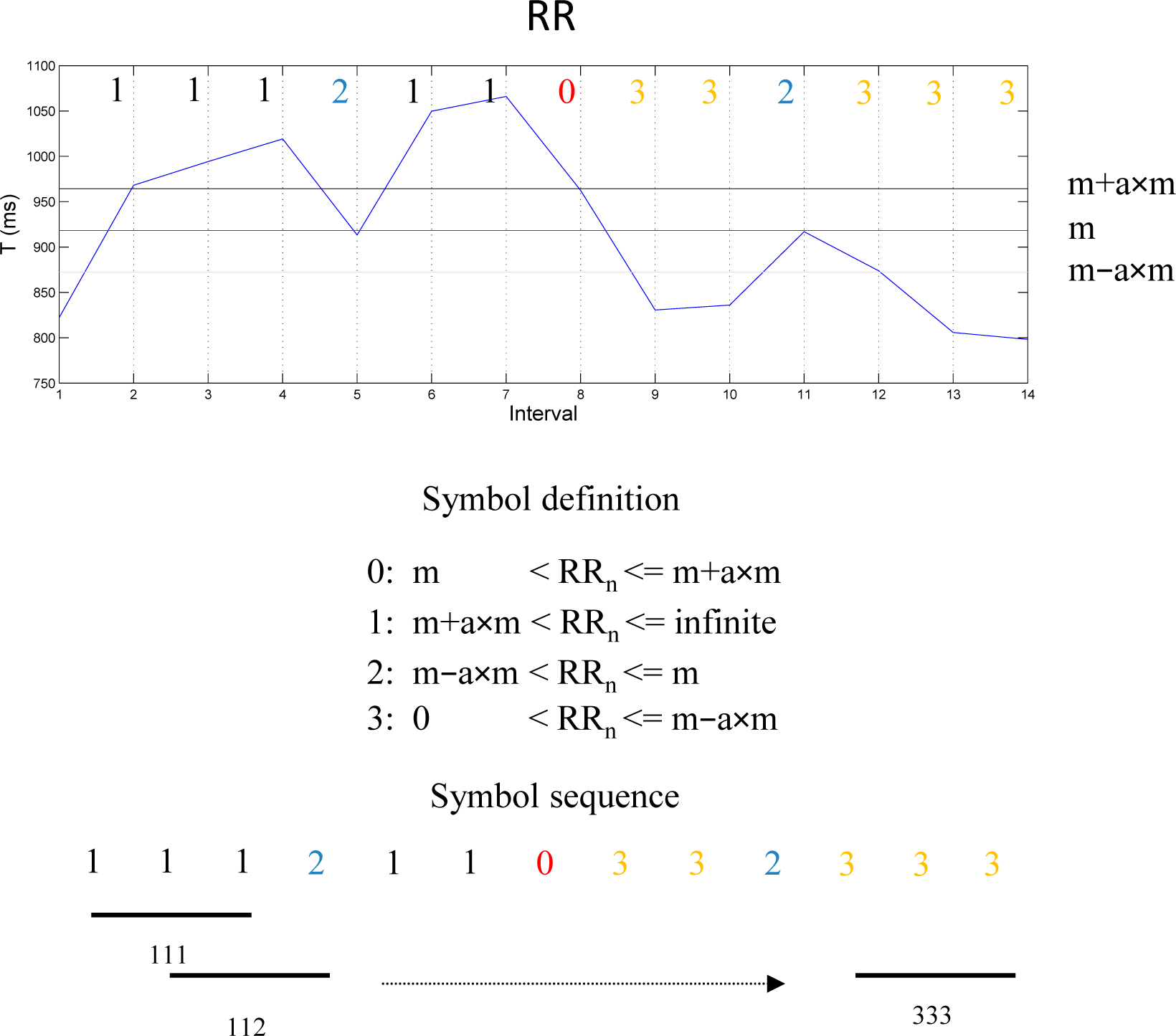
2.7.1. Symbolic Dynamic (SD)

The methods from symbolic dynamics (see Figure 2) are a suitable tool for non-linear HRV analysis and allow its investigation as a complex system [24]. It consists of a transformation of the initial time series of RR-intervals into a sequence of symbols of a given alphabet. While some detailed information is lost in the process, the coarse dynamic behavior can be analyzed more easily.

We investigated the use of words of length 3 (i.e., constructed from three adjacent symbols), obtaining the next word by shifting the time series to the next symbol. The maximum number of possible different words of length three from our given alphabet {0,1,2,3} is equal to 64. The full range of RR intervals is divided into four partitions by using three different levels:

$$\begin{array}{l}{\mathrm{T}}_1=\mathrm{m}\left(1-\mathrm{a}\right)\\ {\mathrm{T}}_2=\mathrm{m}\\ {\mathrm{T}}_3=\mathrm{m}\left(1+\mathrm{a}\right)\end{array}$$

(10)

The transformation into symbols refers to three given levels where m refers to the mean RR-interval and a is a special parameter which is set to 0.05. The symbols are assigned to each RR interval by applying the following rules:

$$\begin{array}{l}\mathrm{if}{\mathrm{T}}_2<\mathrm{RRn}<={\mathrm{T}}_3,\text{then}\mathrm{Sn}=0;\\ \mathrm{if}{\mathrm{T}}_3<\mathrm{RRn},\text{then}\mathrm{Sn}=1;\\ \mathrm{if}{\mathrm{T}}_1<\mathrm{RRn}<{\mathrm{T}}_2,\text{then}\mathrm{Sn}=2;\\ \mathrm{if}0<\mathrm{RRn}<={\mathrm{T}}_1,\text{then}\mathrm{Sn}=3.\end{array}$$

(11)

From the different variables based on linear dynamics and described in [11], we decided to use the following:

-

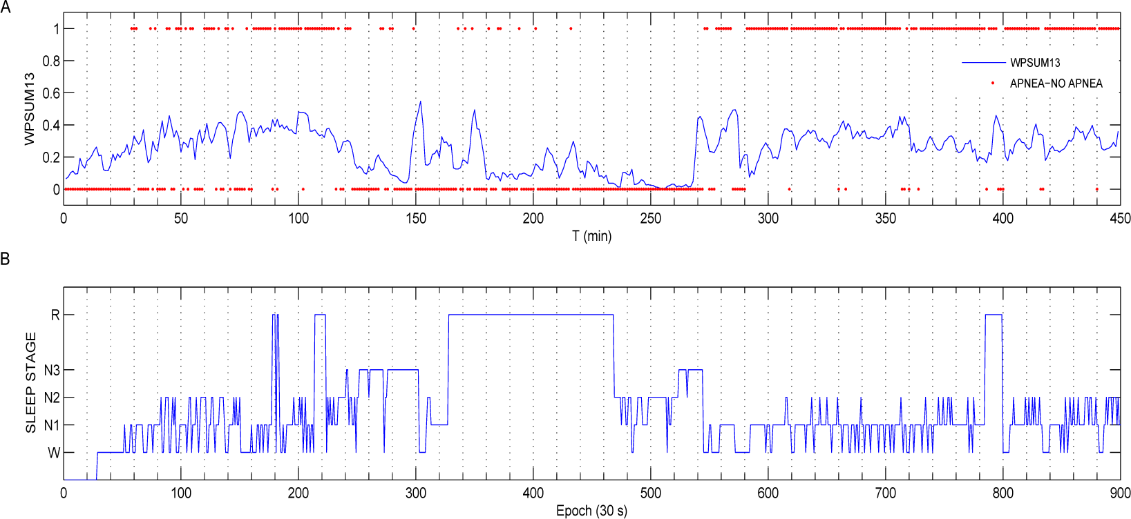
WPSUM13: This variable quantifies the percentage of words which contain the symbols “1” and “3”. This feature is a measure of increased HRV.

-

WPSUM02: This variable quantifies the percentage of words which contain the symbols “0” and “2”. This feature is a measure of decreased HRV.

Entropy measures are very interesting features to evaluate the complexity of time series from the generated distributions of words. Higher values of these entropies are related to increased complexity in the corresponding tachograms and lower values to decreased complexity. Measures based on entropy are presented below:

-

FWSHANNON: Shannon entropy of order k is defined on the basis of the probability distribution p of words of length k [12].

$$H_k=-{\displaystyle \sum _{\omega \in W^k,p\left(\omega \right)>0}p(\omega )\ln p(\omega )}$$

(12)

where ω^k denotes the set of all words of length k.

-

FWRENYI: This is a generalization of Shannon entropy based on the distribution of probability p of length k words and defined by the following expression:

$$H_k=\frac{1}{1-q}\ln \left({\displaystyle \sum _{\omega \in W^k,p(\omega )>0}p{(\omega )}^{(q)}}\right)$$

(13)

where q is a real number greater than zero. The q parameter can be adjusted to weight probabilities differently, for example if q > 1, the words of length k with large probabilities dominantly influence the Renyi entropy. On the other hand if 0 < q <1 the words with small probabilities mainly determine the value of H_k^(q). In our case we have considered these two possibilities using q = 0.25 (FWRENYI0.25) and q = 4 (FWRENYI4). Starting from the word sequences it is possible to derive other sequences which can then be analyzed. The variables which we state in the following are based on this proposal.

-

WSDVAR: This variable is a measure of the variability of the time series calculated from the transformed sequence of words. The resulting sequence of words {ω1,ω2,ω3,…} of Figure 2 is transformed into a sequence $\left\{\overline{s_1,}\overline{s_2,}\overline{s_3,}\dots \right\}$ as described in (14):

$$\overline{s_i}({\omega }_i)=\left\{\begin{array}{l}3if{n}_{13}({\omega }_i)=3\wedge s_{13}({\omega }_i)=\prime 1\prime \\ 2if{n}_{13}({\omega }_i)=2\wedge s_{13}({\omega }_i)=\prime 1\prime \\ 1if{n}_{13}({\omega }_i)=1\wedge s_{13}({\omega }_i)=\prime 1\prime \\ 0if{n}_{13}({\omega }_i)=0\\ -1if{n}_{13}({\omega }_i)=1\wedge s_{13}({\omega }_i)=\prime 3\prime \\ -2if{n}_{13}({\omega }_i)=2\wedge s_{13}({\omega }_i)=\prime 3\prime \\ -3if{n}_{13}({\omega }_i)=3\wedge s_{13}({\omega }_i)=\prime 3\prime \end{array}\right\}i=1,2,3,\dots$$

(14)

where n₁₃(ω_i) represents the number of symbols corresponding to 1 or 3 in the word and s₁₃(ω_i) represents the first occurring symbol, either 1 or 3, in the word ω_i. WSDVAR is defined as the standard deviation of the sequence $\overline{s_i}$.

$$WSDVAR={\left(\frac{{\displaystyle \sum _{i=1}^N{\left(\overline{s_i}({\omega }_i)-\frac{1}{N}{\displaystyle \sum _{i=1}^N\overline{s_i}({\omega }_i)}\right)}^2}}{N-1}\right)}^{1/2}$$

(15)

-

FORBWORDS: This variable counts the so-called forbidden words of length 3. Specifically, the number of words that never occur or do so with very low probability (less than 0.001) is calculated. If the sequence under study is highly complex, we will find few forbidden words. A large number of forbidden words can, on the other hand, imply a much more regular behaviour.

A last set of variables based on symbolic dynamics is used for the analysis of high or low variability. In this case we will consider words of 6 consecutive symbols of a simplified 2-symbol alphabet {0,1}. The symbol “0” is selected when the difference between two successive values is less than a certain threshold, while the symbol “1” represents those exceeding it. The output sequence is determined by the expression:

$$S_{n,w_i}=\left\{\begin{array}{c}\prime 0\prime :{\left|N{N}_n-N{N}_{n-1}\right|}_{w_i}<th\\ \prime 1\prime :{\left|N{N}_n-N{N}_{n-1}\right|}_{w_i}\ge th\end{array}\right\}$$

(16)

where n = 1,2,3,4,5,6, ωi is the i^th word of 6 symbols and the threshold (5, 10, 20 ms).

-

POLVAR: These variables represent the probability that the word “000000” occurs for a specific threshold, thus describing the occurrence of low heart rate variability. We select three versions for analysis: POLVAR5, POLVAR10, POLVAR20, with thresholds of 5, 10 and 20 ms respectively.

-

PHVAR: Oposite to POLVAR, the PHVAR variables represent the probability of the word “111111”, so quantifying high variation in heart rate as defined by thresholds as above (5, 10 and 20 ms) resulting in the PHVAR5, PHVAR10 and PHVAR20 variables.

2.8. Classifier

A linear discriminant analysis (LDA) [25] is used to classify segments in a minute by minute basis into the classes of containing apnea and those that do not. This classifier provides a parametric model that maps the feature inputs to the required output classes and has a set of adjustable parameters that are calculated from the learning data.

The models in this study assumes that the features have a class-dependent multivariate Gaussian distribution:

$$f_k\left(x\right)=\frac{1}{{\left(2\pi \right)}^{\frac{p}{2}}{\left|{\displaystyle {\sum }_k}\right|}^{\frac{1}{2}}}{e}^{-\frac{1}{2}{(x-{\mu }_k)}^T{\displaystyle {\sum }_k{}^{-1}(x-{\mu }_k)}}$$

(17)

where µ_k and ∑k are the mean vector and covariance matrix of each class k (apnea and no-apnea class).

LDA also makes the simplifying assumption that the class covariances are identical ∑k = ∑ for both classes, defining a linear boundary between the classes as:

$${\delta }_k\left(x\right)=x^T{\displaystyle {\sum }_{}^{-1}{\mu }_k-\frac{1}{2}{\mu }_k^T{\displaystyle {\sum }_{}^{-1}{\mu }_k+\log {\pi }_k}}$$

(18)

where π_k is the prior probability of class k.

The parameters of the Gaussian distributions will be estimated from the learning data:

$${\widehat{\pi }}_k=N_k/N$$

(19)

$${\widehat{\mu }}_k={\displaystyle {\sum }_{g_i=k}^{}{x}_i/N_k}$$

(20)

$$\widehat{\mathrm{\Sigma }}={\displaystyle \sum _{k=1}^K{\displaystyle \sum _{g_i=k}\left(x_i-{\widehat{\mu }}_k\right){\left(x_i-{\widehat{\mu }}_k\right)}^T/\left(N-K\right)}}$$

(21)

where N_k is the number of class-k observations.

The LDA will classify one minute segment as apnea if:

$$x^T{\widehat{\mathrm{\Sigma }}}^{-1}\left({\widehat{\mu }}_{ap}-{\widehat{\mu }}_{\mathit{nap}}\right)>\frac{1}{2}{\mu }_{ap}^T{\widehat{\mathrm{\Sigma }}}^{-1}{\widehat{\mu }}_{ap}-\frac{1}{2}{\mu }_{\mathit{nap}}^T{\widehat{\mathrm{\Sigma }}}^{-1}{\widehat{\mu }}_{\mathit{nap}}+\log \left(\frac{N_{\mathit{nap}}}{N}\right)-\log \left(\frac{N_{ap}}{N}\right)$$

(22)

where ${\widehat{\mu }}_{ap}$ and ${\widehat{\mu }}_{\mathit{nap}}$ are the mean vectors of class apnea and no-apnea respectively and on the other hand N_ap and N_nap, the number of apnea and no-apnea vectors.

Finally, LDA assumes normal distribution for both classes. In order to reduce the dynamic range of the variables and approximate them to a gaussian distribution, we applied a logarithmic transformation.

2.9. Global Classification Criterion

Our approach is to classify apnea in minute long segments. With the minute by minute approach, we are able to establish a threshold based on the number of detected apneic minutes. The threshold is defined, taking into consideration the PSG-based AHI definition and our thus calculated m-AHI-tib defined as the number of minutes with events per hour of time in bed. This is in line with previous publications [14,26] and it is highly correlated with the AHI-tib obtained with polygraphy. The LDA provides two outputs. The first one is a one minute by minute quantification of normal respiration or apnea. The second is a global score of the presence of clinically significant apnea which is derived from segment-wise output. A subject is classified globally as apneic if the m-AHI-tib is greater than 10.

2.10. Feature Selection

In order to optimize classification performance, a 50 repeated random sub-sampling validation [27] is used with the learning set in order to find the variables that are most highly correlated with the presence of apnea. On each iteration a random partition of half of the feature vectors is used to train (Rank_train) with the rest then used to test (Rank_test) (Figure 3).

The features are selected greedily, i.e., a classifier is repeatedly trained with all features added individually to the current set, and the best performing set it used for the next round. If the performance does not increase with added features the final feature set is found. After 50 iterations a corresponding number of feature sets have been generated and the features can be ranked by the number of times they were included in those sets.

In a second step (with the features ordered according to their rankings), the mean misclassification error is calculated for an increasing number of features, using a training (Count_train) and a validation set (Count_test), also chosen through random sub-sampling validation in the L set repeated 50 times. The final number of selected features is based on the minimum average error per feature count obtained in this last validation process. Finally, the performance of the classifier is evaluated for the independent 35 recordings (Test set) with the selected features.

3. Results

3.1. Descriptive Statistics

For all one minutes segments and each of the subgroups considered (presence of OSA: apnea/absence of OSA: normal), all oxymetry and RR variables were summarized as median and interquartile ranges. The distribution of the different variables for both groups were compared with the Wilcoxon test.

Table 2. Description of the time and frequency domain HRV variables of the data set as a function of the presence (A) or absence of OSA (NA). Data are expressed as median and interquartile ranges.

Features	A	NA	P
meanNN5m (ms)	917.12 (820.97;995.03)	913.89 (836.84;989.55)	NS
SdNN5m (ms)	63.27 (42.85;89.94)	40.35 (27.42;61.65)	<0.0001
CvNN5m (ms)	0.07 (0.05;0.1)	0.05 (0.03;0.07)	<0.0001
sdaNN1 (ms)	20.04 (12.19;32.19)	14.97 (8.51;27.27)	<0.001
Rmssd (ms)	31.42 (19.9;50.1)	22.78 (14.49;37.35)	<0.0001
pNN20 (%)	0.47 (0.26;0.62)	0.36 (0.14;0.58)	<0.01
pNN30 (%)	0.71 (0.53;0.89)	0.84 (0.6;0.96)	<0.001
pNN50 (%)	0.1 (0.02;0.26)	0.03 (0;0.16)	<0.0001
pNN100 (%)	0.01 (0;0.05)	0 (0;0.02)	<0,001
pNN110 (%)	0.28 (0.2;0.44)	0.35 (0.22;0.55)	NS
pNN120 (%)	0.53 (0.38;0.74)	0.64 (0.42;0.86)	<0.01
pNN150 (%)	0.9 (0.74;0.98)	0.97 (0.84;1)	<0.0001
Shanon	2.47 (2.11;2.78)	2.03 (1.68;2.41)	<0.0001
Renyi025 2.7	(2.37;2.99)	2.34 (2.01;2.69)	<0.0001
Renyi4 2.17	(1.79;2.49)	1.7 (1.36;2.07)	<0.0001
Renyi2	2.31 (1.94;2.63)	1.84 (1.5;2.23)	<0.0001
ULF (s2)	22.08 (6.39;68.77)	15.44 (4.14;55.92)	NS
VLF (s2)	935.2 (406.61;1953.83)	270.45 (112.84;691.04)	<0.0001
LF (s2)	376.71 (165.92;877.88)	151.93 (66.32;362.75)	<0.0001
HF (s2)	110.78 (43.41;292.77)	63.88 (25.07;178.28)	<0.001
P (s2) 1713.15	(767.24;3471.79)	628.22 (283.64;1478.56)	<0.0001
LF/HF	3.51 (2.04;6.34)	2.35 (1.09;4.98)	<0.05
LF/P	0.25 (0.16;0.38)	0.26 (0.17;0.37)	NS
HF/P	0.07 (0.04;0.13)	0.11 (0.05;0.24)	<0.001
VLF/P 0.61	(0.46;0.73)	0.5 (0.34;0.66)	<0.001
ULF/P	0.01 (0;0.04)	0.03 (0.01;0.07)	NS
(ULF+VLF+LF)/P	0.93 (0.87;0.96)	0.89 (0.76;0.95)	<0.001
(ULF+VLF)/P	0.65 (0.48;0.77)	0.56 (0.38;0.73)	<0.001
UVLF (s2)	989.77 (430.6;2043.49)	298.42 (124.49;769.25)	<0.0001
LFn 0.78	(0.67;0.86)	0.7 (0.52;0.83)	<0.05
HFn 0.22	(0.14;0.33)	0.3 (0.17;0.48)	<0.05
NoNNtime (ms)	1053.13 (0;3993.13)	1050.47 (0;4400.96)	NS

summarizes the variables obtained by linear feature extraction methods applied to RR intervals in time and frequency domain.

Table 3. Description of the symbolic dynamics variables of HRV for the whole database in function of the presence (A) or absence of obstructive sleep apnea (NA). Data are expressed as median and interquartile ranges.

Features	A	NA	P
FORBWORD	30 (21;38)	37 (25;43)	<0.0001
FWSHANNON	2.82 (2.51;3.11)	2.65 (2.24;3.08)	<0.001
FWRENYI025	3.33 (3.07;3.59)	3.13 (2.86;3.5)	<0.0001
FWRENYI4	1.95 (1.6;2.29)	1.91 (1.52;2.38)	NS
WSDVAR	1.82 (1.38;2.2)	1.24 (0.77;1.73)	<0.0001
WPSUM02	0.33 (0.14;0.55)	0.59 (0.33;0.82)	<0.0001
WPSUM13	0.26 (0.13;0.41)	0.09 (0.03;0.21)	<0.0001
POLVAR5	0 (0;0.01)	0 (0;0.01)	NS
POLVAR10	0 (0;0.03)	0 (0;0.04)	NS
POLVAR20	0.06 (0.01;0.24)	0.11 (0.01;0.44)	NS
PHVAR5	0.42 (0.23;0.56)	0.32 (0.14;0.53)	<0.01
PHVAR10	0.17 (0.05;0.31)	0.08 (0.01;0.25)	<0.001
PHVAR20 0.02	(0;0.1)	0 (0;0.05)	<0.0001

summarizes the p-values of the variables obtained by non linear feature extraction methods applied to HRV.

WPSUM13 presents the best discriminatory capacity of all the individual symbolic dynamics based variables. Figure 4 shows the dynamic of this variable every minute and the hypnogram for a patient with obstructive sleep apnea who clearly experiences increased heart rhythm. It can be observed bigger values of variable WPSUM13 in minutes with apnea and also in rapid eye movement (REM) and Wake transitions.

Table 4. Description of the variables obtained from oximetry for the whole data set as a function of the presence (A) or absence of obstructive sleep apnea (NA). Data are expressed as median and interquartile ranges.

Features	A	NA	P
var Sat1m	5.229 (2.231;12.737)	0.251 (0.163;0.778)	<0.0001
var Sat5m	6.678 (3.135;15.376)	0.623 (0.259;1.659)	<0.0001
Fb1	1.7 × 10−26 (5 × 10−27;1.2 × 10−25)	4.1 × 10−25 (6.3 × 10−26;4.3 × 10−24)	<0.0001
Fb2	0.054 (0.02;0.121)	0.113 (0.046;0.236)	<0.0001
Fb3	0.04 (0.015;0.087)	0.073 (0.032;0.144)	<0.001
Fb4	0.041 (0.016;0.087)	0.06 (0.025;0.116)	NS
Fb5	0.045 (0.019;0.098)	0.055 (0.023;0.104)	NS
Fb6	0.05 (0.02;0.107)	0.051 (0.022;0.098)	NS
Fb7	0.057 (0.021;0.123)	0.045 (0.018;0.087)	<0.01
Fb8	0.057 (0.022;0.129)	0.037 (0.015;0.073)	<0.01
Fb9	0.047 (0.018;0.109)	0.031 (0.013;0.062)	NS
Fb10	0.032 (0.012;0.075)	0.026 (0.01;0.052);	NS
Fb11	0.021 (0.008;0.051)	0.021 (0.008;0.043)	NS
Fb12	0.016 (0.006;0.036)	0.017 (0.007;0.036)	NS
Fb13	0.012 (0.005;0.026)	0.014 (0.005;0.031)	NS
Fb14	0.009 (0.004;0.021)	0.011 (0.004;0.025)	NS
Fb15	0.008 (0.003;0.018)	0.01 (0.004;0.022)	NS
Fb16	0.007 (0.003;0.016)	0.008 (0.003;0.019)	NS
Fb17	0.006 (0.002;0.014)	0.007 (0.003;0.016)	NS
Fb18	0.005 (0.002;0.012)	0.006 (0.002;0.014)	NS
Fb19	0.004 (0.002;0.009)	0.005 (0.002;0.012)	<0.05
Fb20	0.003 (0.001;0.007)	0.004 (0.002;0.01)	NS

summarizes the p-values of the variables obtained from oximetry. Variance of the signals and some spectral based features present a relevant p-value.

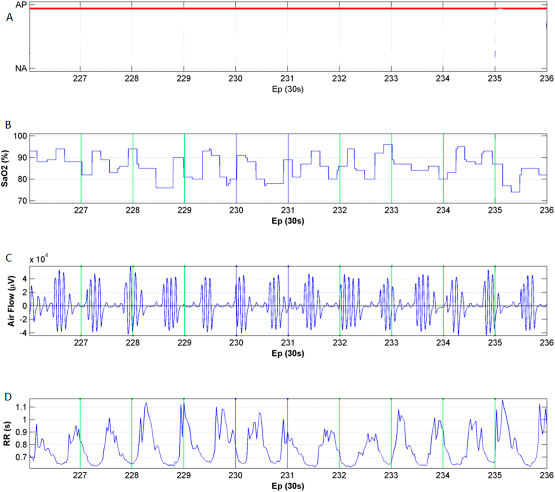
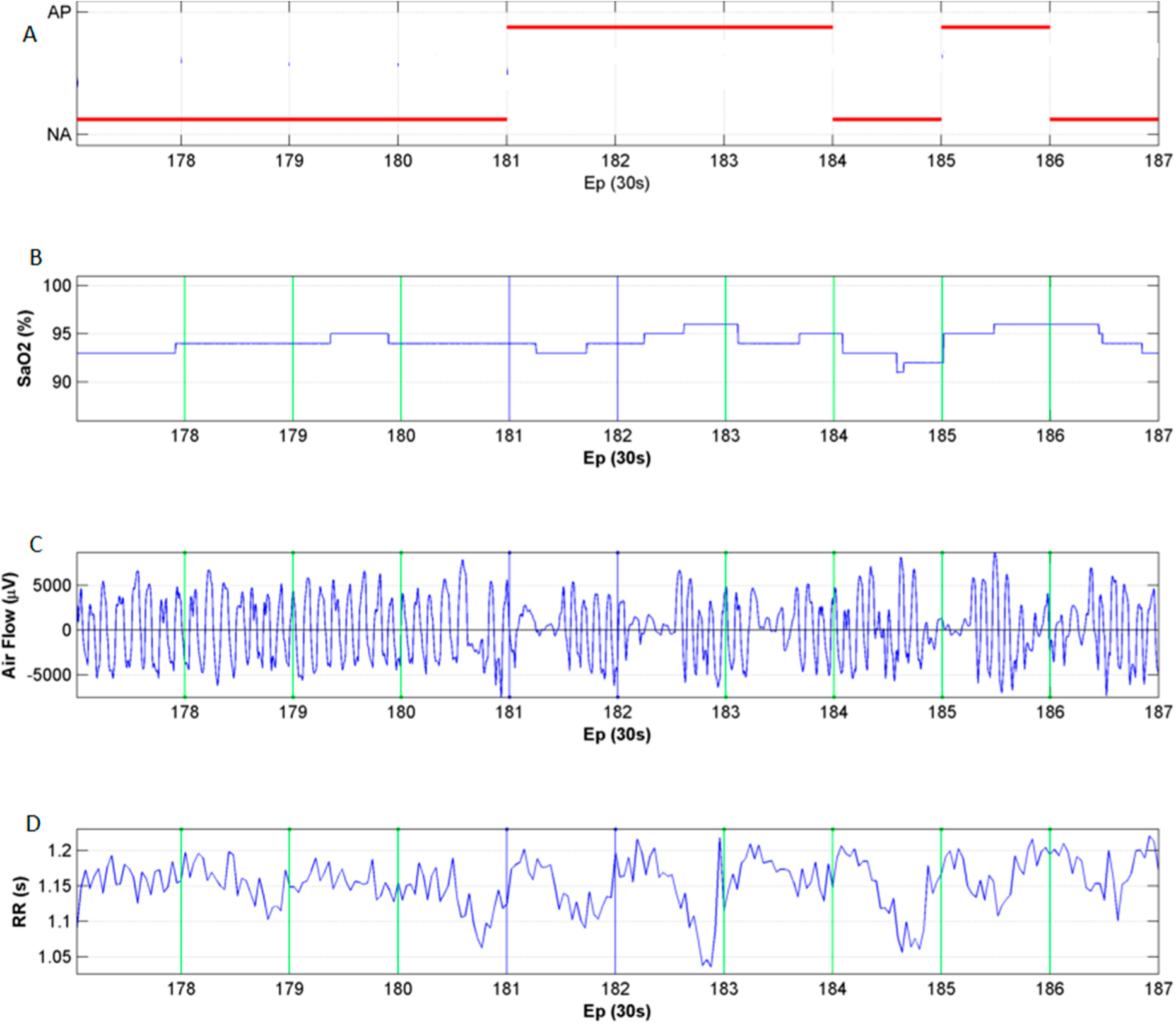
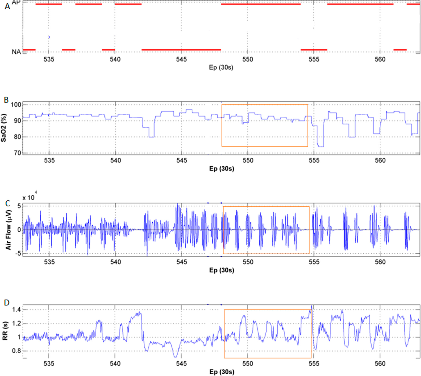
3.2. HRV and Oximetry Pattern Obtained in Presence of OSA

In Figure 5 measurements for a patient with OSA is presented, with 10 epochs of 30 seconds length. In Figure 5a, the manual scoring indicates the presence of a respiratory disturbance. Oximetry, air flow obtained by thermistor and RR intervals from EKG, is represented in Figure 5b–d, respectively.

In some segments with obstructive sleep apnea, heart rate shows occurrence of both, first presenting bradycardia during the apneic phase, followed by tachycardia during the arousal and activation of the upper airway muscle that finally allows airflow into the lungs. A resulting low frequency periodic pattern can be observed in Figure 5d.

Deep oxygen desaturations can also be observed in oximetry signal. In patients with severe obstructive sleep apnea, these desaturations are observed as a periodic oximetry signals where a low frequency component could be obtained as in Figure 5b. A recovery of the oximetry value is obtained shortly after the upper airway muscle allows airflow into the lungs. This patter strengthens our idea of using not only the variance of the signal in one minute segment but also the variance in five minutes segments or even a spectral analysis in wider segments windows (in our case, five minutes).

In some cases, certain respiratory pauses do not produce a clear pattern in the oximetry signal. This is the case presented in Figure 6 where short time apnea/hipopneas do not produce desaturations.

In Figure 7 it is possible to appreciate another example from the same patient as in Figure 6 where short events (in the orange rectangle) are linked to increased heart rate variability but not to oxygen desaturations and longer breathing events after epoch 555 are associated to increased heart rate variability but also to desaturations in the oximetry signal. In both cases, tachycardia and bradycardia are observable in the RR series dynamic.

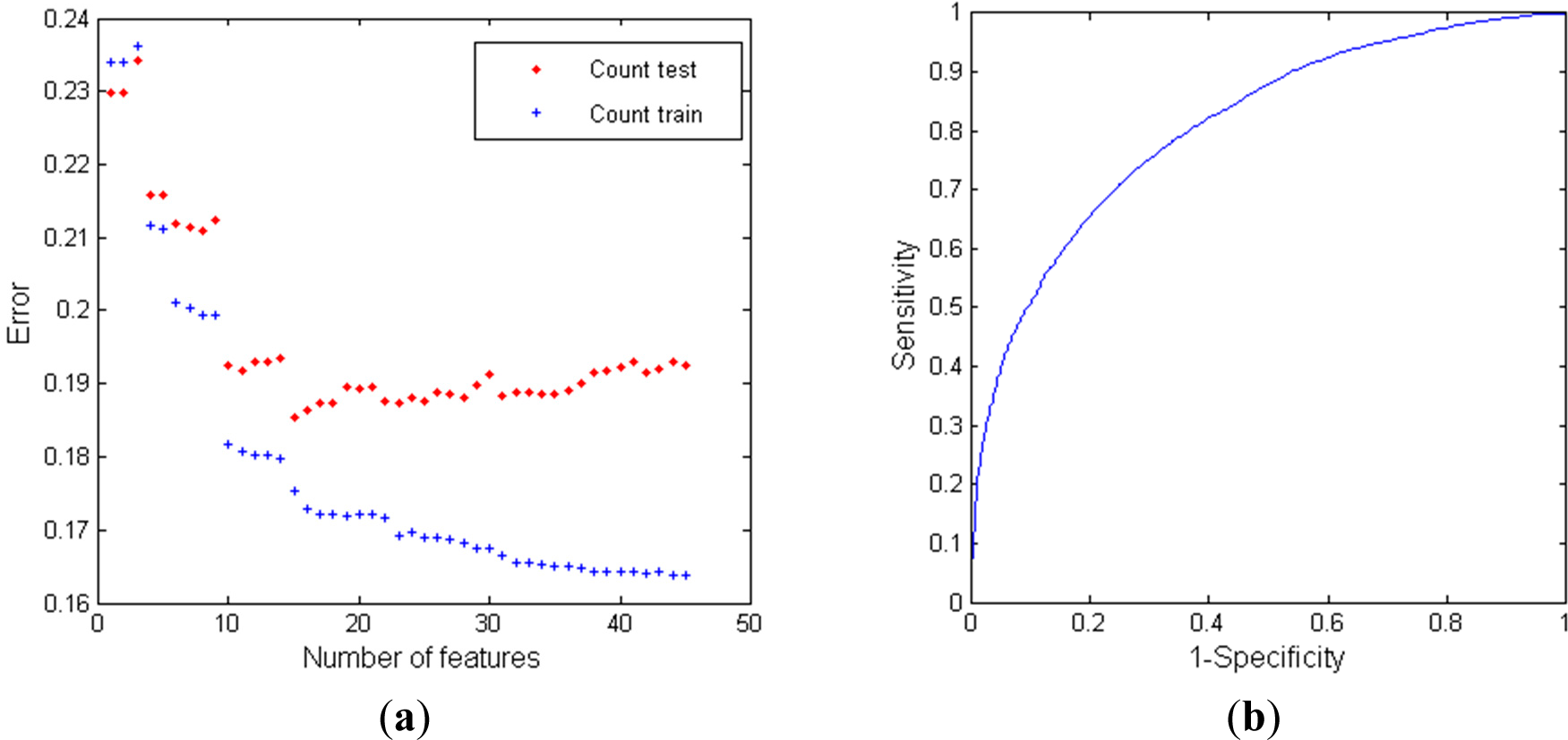
3.3. Results of the OSA Detection System Based on LDA Classifier

The machine learning performance is evaluated using the features obtained from RR series, oxymetry and the combination of both. For all these combinations, a LDA classifier is evaluated through a ROC presentation and a feature selection process is proposed. The data analysis was carried out in MatLab R2012a.

3.3.1. Classifier Performance using RR Intervals

Variables obtained from RR intervals in time and frequency domain (TD, FD) and from symbolic dynamics (SD) have been studied in order to evaluate the performance of the LDA classifier. In Figure 8a, misclassification error for the Count_test data in function of number of features is represented with red asterisks. In case of Count_train data, misclassification error is presented in blue crosses. In this example, 15 features obtain the best results being selected the following variables in the following order of relevance (meanNN_5m, ULF/P, ULF, WPSUM13, sdaNN1, Renyi4, Renyi025, Shannon, LF/P, HFn, Renyi2, sdNN_5m, POLVAR5, (ULF + VLF)/P and POLVAR20).

The cut-off corresponding to the point of ROC curve (Figure 8b) that minimizes the distance between the curve and the upper left corner (the sum of sensitivity and specificity is maximal) was chosen with the L set.

Table 5. Performance of the classifier for the different selected variables. * Results of global classification considering all the validation dataset except borderline subjects.

Features	Signals	n	Variables	Acc %	Se %	Sp %	AUC %	Gc %	Gc %*
TD + FD + SD	RR	15	meanNN5m, ULF/P, ULF, WPSUM13, sdaNN1, Renyi4, Renyi025, Shanon, LF/P, HFn, Renyi2, sdNN5m, POLVAR5, (ULF+VLF)/P, POLVAR20	79.4	42.4	94.3	80.9	71.4	81.8
Var + Fbank	SpO2	19	var Sat1m, Fb2, Fb9, Fb8, Fb11, Fb20, Fb7, Fb12, Fb1, Fb18, Fb4, Fb5, Fb13, Fb17, Fb14, Fb15, Fb16, Fb6, Fb10	86.5	75.6	91	89.8	91.4	97
TD + FD + SD + (Var + Fbank)	SpO2 + RR	33	var Sat1m, Fb2, Fb9, LF/HF, Fb3, (ULF+VLF+LF)/P, Fb8, sdaNN1, Fb12, FORBWORD, Fb11, var Sat5m, Fb1, pNN120, ULF/P, POLVAR5, LF/P, FWRENYI025, POLVAR10, Fb7, Shanon, HF, Renyi2, sdNN, Fb20, cvNN5m, Fb6, noNNtime, Fb16, Renyi025, pNN30, Renyi4, pNN110	86.9	73.4	92.3	91.9	94.3	100

summarizes quantitatively the performance of the recognition system for the T set and for the best combination of variables. The accuracy is 79.4% (AUC = 81), sensitivity being 42.4% and specificity 94.3%. Although specificity is very good, a poor sensitivity is obtained. Global classification performance is 71.4%. When borderline are not used, 81.8% of the patients are correctly discriminated in the global classification task.

3.3.2. Classifier Performance using Oximetry

For each of the selected variables obtained from oximetry, and in the order of relevance which are extracted, the misclassification error is obtained and represented in Figure 9a. For this case, optimum number of features (n = 19) are selected according to misclassification error obtained with the Count_test data. The features are the following: var Sat_1m, Fb2, Fb9, Fb8, Fb11, Fb20, Fb7, Fb12, Fb1, Fb18, Fb4, Fb5, Fb13, Fb17, Fb14, Fb15, Fb16, Fb6 and Fb10. An optimum decision threshold is obtained and the ROC curve presented in Figure 9b.

Table 5 summarizes the performance of the LDA classifier for the T set, with an accuracy of 86.5% (AUC = 89.8). The sensitivity obtained is 75.6% and specificity is 91%. Global classification performance is 91.4%. When borderline are not used, global classification performance is 97%. From the 33 test patients (10 control and 23 apneas), 32 are correctly classified according to the criterion of m-AHI-tib = 10 as threshold. The patient that is not correctly classified is a patient with respiratory events without clear desaturation and with some polygraphic traces represented in Figures 8 and 9.

3.3.3. Classifier Performance using RR Series and Oximetry

Figure 10a,b represents the misclassification error for the Count_train (red asterisks) and Count_test (blue crosses) data for one thing and ROC curve, on the other hand, when a combination of RR series and oximetry variables are involved.

Variables selected are the following in order of ranking: var Sat_1m, Fb2, Fb9, LF/HF, Fb3, (ULF + VLF + LF)/P, Fb8, sdaNN1, Fb12, FORBWORD, Fb11, var Sat_5m, Fb1, pNN120, ULF/P, POLVAR5, LF/P, FWRENYI025, POLVAR10, Fb7, Shanon, HF, Renyi2, sdNN, Fb20, cvNN, Fb6, noNNtime, Fb16, Renyi025, pNN30, Renyi4 and pNN110.

The features extracted from the oximetry seem to be significant according to the order of relevance, such as the variance in one minute segments, although the inclusion of other variables obtained from the spectral analysis of oximetry in five minutes segments are also quite relevant.

For this combination of variables Table 5 summarizes the performance of the classifier. The accuracy has increased from 86.5% (only oximetry) to 86.9% (a combination of variables of RR series and oximetry) with a sensitivity of 73.4% and specificity of 93.3%.

In this case, global classification performance is 94.3%. When borderline are not used, the global classification rate is 100%. The patient that was previously globally misclassified is now classified correctly. The changes in the dynamic of the HRV could be helping to the classifier to detect events with poor desaturations as in this case.

4. Discussion

The performance of an automatic diagnostic system based on oximetry and RR series has been evaluated. In addition to respiratory events, other variables related to high blood pressure or cardiovascular or respiratory disorders may affect the autonomic regulatory system and may be respresented in HRV. We showed that the RR series can be a complementary source of information to oximetry and can in combination improve the performance of a low cost diagnosis system for apnea.

Previously oximetry has demonstrated its high specificity in the detection of sleep breathing events, however in some cases, as we also observe in this study, apnea does not always present a clear pattern of oxygen desaturation. For example, short time events scored as apnea or hypopnea by the expert may fall into this category.

According to the feature selection process, the variables obtained from oximetry seems to be highly significant indicators, especially the variance obtained in one and five minutes segments, but also the variables related to the spectral analysis of oximetry.

Regarding variables obtained from RR series, both linear and nonlinear features are selected in the final classifier that integrates oximetry and RR series. Some variables obtained from symbolic dynamic are also statistically significant according to the results. This is the case of FORBWORD and WPSUM13, although this last variable is only included in the classifier that exclusively consisted of RR series features. The inclusion of WPSUM13 variable allows us to obtain information about the higher variability of the heart rhythm highly correlated with the presence of OSA.

A question remains, in what the reason is to not experience oxygen desaturation for short apnea events? One possibility could be the hemoglobin dissociation curve. The sigmoid representation of the curve could indicate that the percentage of SpO2 would not start to decrease until a marked reduction in the partial oxygen pressure occurs, sometime after the airflow obstruction. There would not be enough time to desaturate in short events. On the other hand, this curve could be displaced due to other factors such as pH, temperature and 2,3-diphosphoglycerate (2,3-DPG) levels, which are specific to each person and would explain the different responses in airflow obstructions of the same duration.

An explanation could be also the averaging of pulses in the oximetry hardware to calculate oxygen saturation. Always a decent number of pulses, usually between three and 12, is needed to calculate an oxygen saturation value. In the case of short events, there may be too few pulses that a relevant desaturation is noted. For example, 12 pulses represent roughly 10 s in time. So this is like a low-pass filter to the true oxygen saturation.

Other groups have previously scored the presence of OSA based on oximetry and HRV, and in a few cases also on a combination of oximetry and HRV. Most of the studies tend to classify the presence of apnea globally based on an AHI threshold. For example, Marcos et al. [28] extracted spectral and linear features obtained from oximetry with four different classifiers. They achieved a maximum accuracy of 86.7% (88.1% sensitivity and 84.8% sensitivity) on a dataset of 187 subjects (113 of them used to validate the algorithm), with a definition of apnea using an AHI of 10. Alvarez et al. [29] achieved an accuracy of 89.7% (sensitivity of 92% and specificity 85.4%, n = 148) separating apneic patients from normal ones using the same AHI limit with a LR model on features extracted from the oximetry in time and frequency domain.

In a more recent publication, Alvarez et al [30] extracted different linear and non linear features from oximetry trained with 148 subjects and validated on two different databases. An accuracy of 85.2% is achieved for a database of 101 subjects and 88.7% for a different database of 71 subjects in this global classification task.

Only a few studies have been published that have tried to detect the apneic/hypopneic events on a minute by minute basis. In this sense Xie et al. [31] studied a dataset of 25 subjects with HRV and oximetry data, reaching an accuracy of 84.40% (if used with 150 features, reducing to 83.26% when only 39 features were considered). A work reported by Burgos et al. [32] has achieved an accuracy of 93%, but on a very limited database of 8 subjects.

If one would try to compare to studies using all available data from a polygraphic recording, Masa et al. [33] studied a dataset of 348 patients, obtaining a sensitivity of 87% and specificity of 86% in global subject classification targeting subjects with an AHI > 10.

As opposed to many previous publications, our approach is to classify apnea in minute long segments. With this minute by minute approach, we can establish a threshold based on the number of detected apneic minutes. In order to determine the final value of this approach, the cardiovascular consequences of sleep apnea need to be tested against this measure.

It is not easy to establish comparisons with other results due to the use of different datasets in different conditions. That aside, our approach performs well when compared with other methods in a per-subject global OSA diagnosis classification and also in a minute by minute apnea location task.

One limitation of our study is the absence of subjects with cardiac disorders that we would expect to have an impact on the reliability of the feature detection and in general using a population selected among individuals with symptoms suggesting OSA. Moreover the absence of subjects between 5 and 10 events per hour is a limitation that also should be taking into consideration.

Some other issues remain open for future work. For example, the use of other entropy-based features [34]. More in depth considerations about harmonic phenomena and/or the asynchronous increments and decrements of RRI during apneas should be performed. For instance, it is possible to identify numerous small bands located in VLF, LF, and HF regions that may need special attention and the properties of additional methods for spectral analysis must be studied (complex demodulation, wavelets, Cohen’s class time-frequency representations, etc.) if they are able to account for these. We also plan to work others techniques as bootstrapping as an alternative to the random subsampling used in this work. Additionally, recent studies [35] have shown that women with OSA may be more easily detected than men when using RR time series. In future studies we will take into account this aspect considering the gender to carry out a differentiated learning and validation process.

References

1. Ravelo-Garcia, A.; Navarro-Mesa, J.; Hernádez-Pérez, E.; Martin-González, S.; Quintana-Morales, P.; Guerra-Moreno, I.; Juliá-Serdá, G. Cepstrum Feature Selection for the Classification of Sleep Apnea-Hypopnea Syndrome based on Heart Rate Variability, Proceedings of the IEEE Computing in Cardiology Conference (CinC), Zaragoza, Spain, 22–25 September 2013; pp. 959–962.
2. Ravelo, A.; Travieso, C.; Lorenzo, F.; Navarro, J.; Martin, S.; Alonso, J.; Ferrer, M. Application of support vector machines and gaussian mixture models for the detection of obstructive sleep apnoea based on the RR series. WSEAS Trans. Comput. 2006, 5, 121–124. [Google Scholar]
3. Park, J.G.; Ramar, K.; Olson, E.J. Updates on definition, consequences, and management of obstructive sleep apnea. Mayo Clin. Proc. 2011, 86, 549–555. [Google Scholar]
4. Berry, R.B.; Budhiraja, R.; Gottlieb, D.J.; Gozal, D.; Iber, C.; Kapur, V.K.; Marcus, C.L.; Mehra, R.; Parthasarathy, S.; Quan, S.F.; et al. Rules for scoring respiratory events in sleep: Update of the 2007 AASM manual for the scoring of sleep and associated events. J. Clin. Sleep Med. 2012, 8, 597–619. [Google Scholar]
5. Moser, D.; Anderer, P.; Gruber, G.; Parapatics, S.; Loretz, E.; Boeck, M.; Kloesch, G.; Heller, E.; Schmidt, A.; Danker-Hopfe, H.; et al. Sleep classification according to AASM and Rechtschaffen & Kales: Effects on sleep scoring parameters. Sleep 2009, 32, 139–149. [Google Scholar]
6. Ruehland, W.R.; O’Donoghue, F.J.; Pierce, R.J.; Thornton, A.T.; Singh, P.; Copland, J.M.; Stevens, B.; Rochford, P.D. The 2007 AASM recommendations for EEG electrode placement in polysomnography: Impact on sleep and cortical arousal scoring. Sleep 2011, 34, 73–81. [Google Scholar]
7. Deutsch, P.; Simmons, M.; Wallace, J. Cost-effectiveness of split-night polysomnography and home studies in the evaluation of obstructive sleep apnea syndrome. J. Clin. Sleep Med. 2006, 2, 145–153. [Google Scholar]
8. Chiner, E. Approach to the cost of polysomnography in a spanish hospital. Int. J. Pulmon. Med. 2001, 2(2). [Google Scholar]
9. Lévy, P.; Pépin, J.L.; Deschaux-Blanc, C.; Paramelle, B.; Brambilla, C. Accuracy of Oximetry for Detection of Respiratory Disturbances in Sleep Apnea Syndrome. Chest 1996, 109, 395–399. [Google Scholar]
10. Coccagna, G.; Lugaresi, E. Arterial blood gases and pulmonary and systemic arterial pressure during sleep in chronic obstructive pulmonary disease. Sleep 1978, 1, 117–124. [Google Scholar]
11. Wessel, N.; Voss, A.; Malberg, H.; Ziehmann, C.; Voss, H.U.; Schirdewan, A.; Meyerfeldt, U.; Kurths, J. Nonlinear analysis of complex phenomena in cardiological data. Herzschr. Elektrophys. 2000, 11, 159–173. [Google Scholar]
12. Voss, A.; Kurths, J.; Kleiner, H.J.; Witt, A.; Wessel, N.; Saparin, P.; Osterziel, K.J.; Schumann, R.; Dietz, R. The application of methods of non-linear dynamics for the improved and predictive recognition of patients threatened by sudden cardiac death. Cardiovasc. Res. 1996, 31, 419–433. [Google Scholar]
13. Penzel, T.; Moody, G.B.; Mark, R.G.; Goldberger, A.L.; Peter, J.H. The Apnea-ECG Database. Comput. Cardiol. 2000, 27, 255–258. [Google Scholar]
14. Ravelo-García, A.G.; Navarro-Mesa, J.L.; Murillo-Díaz, M.J.; Julia-Serda, G. Application of RR Series and Oximetry to a Statistical Classifier for the Detection of Sleep Apnoea/Hipopnoea, Proceedings of the IEEE Computers in Cardiology Conference 2004 (CinC), Chicago, IL, USA, 19–22 September 2004; pp. 305–308.
15. Trimer, R.; Cabidu, R.; Sampaio, L.L.M.; Stirbulov, R.; Poiares, D.; Guizilini, S.; Bianchi, A.M.; Costa, F.S.M.; Mendes, R.G.; Delfino, A., Jr.; et al. Heart rate variability and cardiorespiratory coupling in obstructive sleep apnea: Elderly compared with young. Sleep Med. 2014, 15, 1324–1331. [Google Scholar]
16. Maeder, M.T. More on heart rate variability in obstructive sleep apnea: Confusion on a higher level or first step to unravel the cardiovascular mystery of the sleep apnea patient? Sleep Breath. 2014, 18, 233–234. [Google Scholar]
17. Kleiger, R.E.; Bosner, M.S.; Rottman, J.N.; Stein, P.K. Time-domain measurements of heart rate variability. J. Ambul. Monit. 1992, 10, 487–498. [Google Scholar]
18. Wessel, N.; Malberg, H.; Bauernschmitt, R.; Kurths, J. Nonlinear methods of cardiovascular physics and their clinical applicability. Int. J. Bifurcat. Chaos. 2007, 17, 3325–3371. [Google Scholar]
19. Bigger, J.T.; Fleiss, J.L.; Steinman, R.C.; Rolnitzky, L.M.; Kleiger, R.E.; Rottman, J.N. Frequency domain measures of heart period variability and mortality after myocardial infarction. Circulation 1992, 85, 164–171. [Google Scholar]
20. Ravelo-García, A.G.; Casanova-Blancas, U.; Martín-González, S.; Hernández-Pérez, E.; Guerra-Moreno, I.; Quintana-Morales, P.; Wessel, N.; Navarro-Mesa, J.L. An Approach to the Enhancement of Sleep Apnea Detection by means of Detrended Fluctuation Analysis of RR intervals. Comput. Cardiol. 2014, 41, 905–908. [Google Scholar]
21. Hayano, J.; Barros, A.K.; Kamiya, A.; Ohte, N.; Yasuma, F. Assessment of pulse rate variability by the method of pulse frequency demodulation. BioMed. Eng. Online. 2005, 4. [Google Scholar] [CrossRef]
22. Task Force of the European Society of Cardiology, the North American. Society of Pacing, and Electrophysiology. Heart rate variability: Standards of measurement, physiological interpretation, and clinical use. Circulation 1996, 93, 1043–1065.
23. Ravelo-García, A.G.; Saavedra-Santana, P.; Juliá-Serdá, G.; Navarro-Mesa, J.L.; Navarro-Esteva, J.; Álvarez-López, X.; Gapelyuk, A.; Penzel, T.; Wessel, N. Symbolic dynamics marker of heart rate variability combined with clinical variables enhance obstructive sleep apnea screening. Chaos 2014, 24, 024404. [Google Scholar]
24. Wessel, N.; Riedl, M.; Kurths, J. Is the normal heart rate “chaotic” due to respiration? Chaos 2009, 19, 028508. [Google Scholar]
25. Hastie, T.; Tibshirani, R. Generalized additive models. Stat. Sci. 1986, 1, 297–310. [Google Scholar]
26. Al-Angari, H.M.; Sahakian, A.V. Automated recognition of obstructive sleep apnea syndrome using support vector machine classifier. IEEE Trans. Inf. Technol. Biomed. 2012, 16, 463–468. [Google Scholar]
27. Bouckaert, RR.; Frank, E. Evaluating the replicability of significance tests for comparing learning algorithms. In Advances in Knowledge Discovery and Data Mining, Proceedings of the 8th Pacific-Asia Conference, PAKDD 2004, Sydney, Australia, 26–28 May 2004; Dai, H., Srikant, R., Zhang, C., Eds.; Springer: Berlin/Heidelberg, Germany, 2004; 3056, pp. 3–12. [Google Scholar]
28. Marcos, J.V.; Hornero, R.; Álvarez, D.; del Campo, F.; Zamarrón, C. Assessment of four statistical pattern recognition techniques to assist in obstructive sleep apnoea diagnosis from nocturnal oximetry. Med. Eng. Phys. 2009, 31, 971–978. [Google Scholar]
29. Alvarez, D.; Hornero, R.; Marcos, J.V.; del Campo, F. Multivariate analysis of blood oxygen saturation recordings in obstructive sleep apnea diagnosis. IEEE Trans. Biomed. Eng. 2010, 57, 2816–2824. [Google Scholar]
30. Alvarez, D.; Hornero, R.; Marcos, J.V.; Wessel, N.; Penzel, T.; del Campo, F. Assessment of feature selection approaches to enhance information from overnight oximetry in the context of sleep apnea diagnosis. Int. J. Neural Syst. 2013, 23. [Google Scholar] [CrossRef]
31. Xie, B.; Minn, H. Real-Time Sleep Apnea Detection by Classifier Combination. IEEE Trans. Inf. Technol. Biomed. 2012, 16, 469–477. [Google Scholar]
32. Burgos, A.; Goñi, A.; Illarramendi, A.; Bermúdez, J. Real-Time Detection of Apneas on a PDA. IEEE Trans. Inf. Technol. Biomed. 2010, 14, 995–1002. [Google Scholar]
33. Masa, J.F.; Corral, J.; Pereira, R.; Duran-Cantolla, J.; Cabello, M.; Hernández-Blasco, L.; Monasterio, C.; Alonso, A.; Chiner, E.; Rubio, M.; et al. Effectiveness of home respiratory polygraphy for the diagnosis of sleep apnoea and hypopnoea syndrome. Thorax 2011, 66, 567–573. [Google Scholar]
34. Ravelo-García, A.G.; Navarro-Mesa, J.L.; Casanova-Blancas, U.; Martin-Gonzalez, S.; Quintana-Morales, P.; Guerra-Moreno, I.; Canino-Rodríguez, J.M.; Hernández-Pérez, E. Application of the Permutation Entropy over the Heart Rate Variability for the Improvement of Electrocardiogram-based Sleep Breathing Pause Detection. Entropy 2015, 17, 914–927. [Google Scholar]
35. Gutiérrez-Tobal, G.C.; Álvarez, D.; Gomez-Pilar, J.; del Campo, F.; Hornero, R. Assessment of Time and Frequency Domain Entropies to Detect Sleep Apnoea in Heart Rate Variability Recordings from Men and Women. Entropy 2015, 17, 123–141. [Google Scholar]
Figure 1. Oximetry signal presented in epoch of 30 s. The graphic shows the evolution of SpO2 signal between epoch 785 and epoch 835.
Entropy 17 02932f1
Figure 2. Example of extraction of symbols from RR intervals and the extraction of word sequences from the symbols series.
Entropy 17 02932f2
Figure 3. Schematic representation of the partition of the database to select features.
Entropy 17 02932f3
Figure 4. WPSUM13 and hypnogram for an apnea patient. (a) represents the dynamic of the variable WPSUM13 every minute. In red asterisk format, the apnea score for every minute indicating the presence of apnea (value = 1) or absence of apnea (value = 0) is presented. Generally, larger values for the variable WPSUM13 are observed for minutes with OSA present. (b) represents the hypnogram indicating the different sleep stages, wakefulness (stage W), light sleep (stages N1 and N2), deep sleep (stage N3) and rapid eye movement (REM) sleep (stage R).
Entropy 17 02932f4
Figure 5. Example of the dynamics in the polygraph for 10 epochs of 30 s for a patient with clear breathing pauses in the entire presented segment. It is possible to observe deep desaturations and the typical bradycardia and tachycardia pattern in RR intervals. (a) represents the score (presence of apnea (AP) or absence of apnea (NA) classified by the expert for every 30 s epoch. (b) represents the oxymetry signal indicating clear desaturations in presence of sleep breathing pauses during the entire segment presented. (c) represents the air flow measured with a thermistor. Finally (d) represents a clear pattern of bradycardia and tachycardia in RR intervals.
Entropy 17 02932f5
Figure 6. Example of the dynamics in the polygraph for a patient with short breathing pauses without associated oxygen desaturations. (a) represents the score (presence of apnea (AP) or absence of apnea (NA) classified by the expert in every 30 seconds epoch. (b) represents the oxymetry signal without deep desaturations in presence of events, for instance between the epoch 181 and 184. (c) represents the air flow measured with a thermistor where it is possible to appreciate shorter events than in Figure 5. Finally (d) represents a pattern of bradycardia and tachycardia in the instants in which the events appear, for example between epoch 181 and 184.
Entropy 17 02932f6
Figure 7. Example of the dynamics in the polygraph for the same patient as in Figure 6 where can be observed short breathing pauses indicated by an orange rectangle which do not produce deep desaturations whereas deeper desaturations are detected in longer events (epoch 556 to 561). (a) represents the presence of apnea (AP) or absence of apnea (NA) classified by the expert for every 30 seconds epoch. (b) represents the oximetry signal. (c) represents the airflow measured with a thermistor where it is possible to appreciate short events (indicated by the orange rectangle) and longer events (epoch 556 to 561). Finally (d) represents a pattern of tachycardia and bradycardia in short and longer events.
Entropy 17 02932f7
Figure 8. (a) Evaluation of misclassification error for variables obtained from RR series with LDA classifier. Misclassification error for Count_test data shown as red asterisks and error for the Count_train data shown in blue crosses. (b) represents the obtained ROC curve.
Entropy 17 02932f8
Figure 9. (a) Evaluation of misclassification error for variables obtained from oximetry with LDA. Misclassification error for Count_test data shown as red asterisks and the error for the Count_train data is shown as blue crosses. (b) represents the obtained ROC curve.
Entropy 17 02932f9
Figure 10. (a) Evaluation of misclassification error for variables obtained from oximetry and HRV with LDA classifier. Misclassification error for Count_test data shown as red asterisks and the error for the Count_train data is shown as blue crosses. (b) represents the obtained ROC curve.
Entropy 17 02932f10