Path Planning of Pattern Transfer Based on Dual-Operator and a Dual-Population Ant Colony Algorithm for Digital Mask Projection Lithography


Abstract
:1. Introduction
2. Methods
2.1. ACS Algorithm
2.2. Improvement Strategy
2.2.1. Self-Adaptive Ant Colony Division
2.2.2. Feedback Operator
2.2.3. Load Operator
2.3. Self-Adaptive Dual-Population Ant Colony
2.3.1. Convergence Rate Optimization
2.3.2. Optimization of Solutions
2.3.3. Algorithm Flow
3. Results and Discussion
3.1. Algorithm Simulation and Discussion
3.1.1. Parameter Setting
3.1.2. Simulation Results and Analysis
Comparison with Simulation Results of Classical ACO Algorithms
Comparison with Simulation Results of Other ACO Algorithms
3.2. Verification Experiments and Discussion
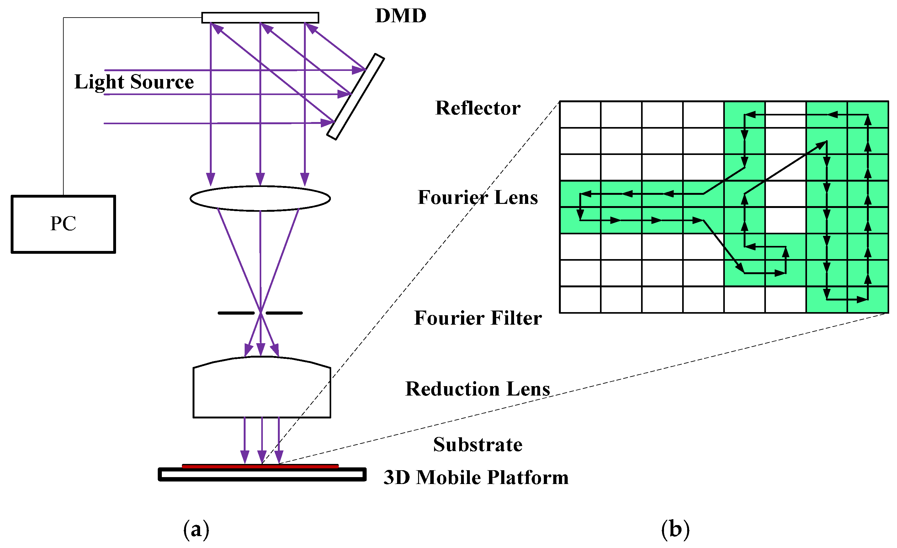
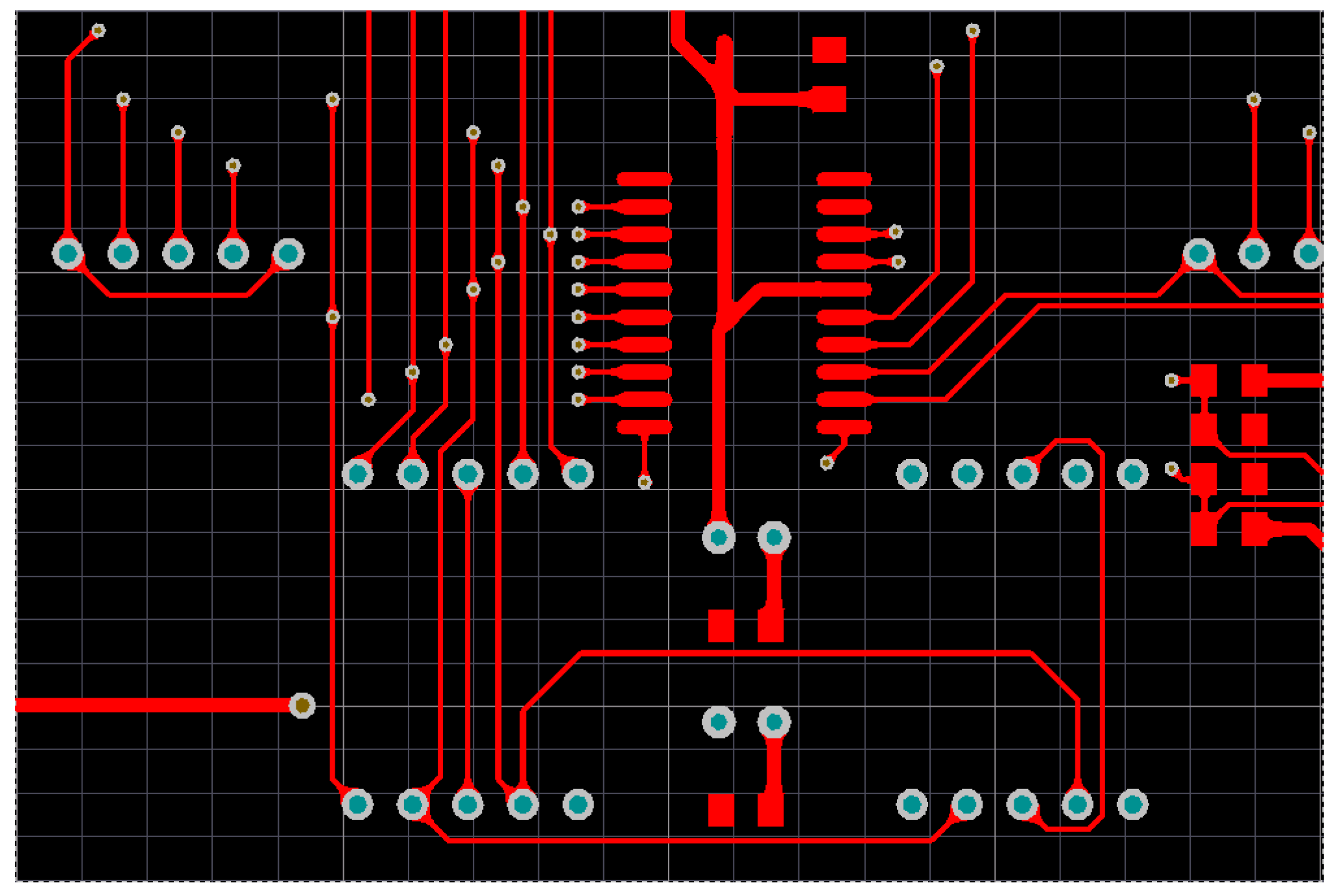
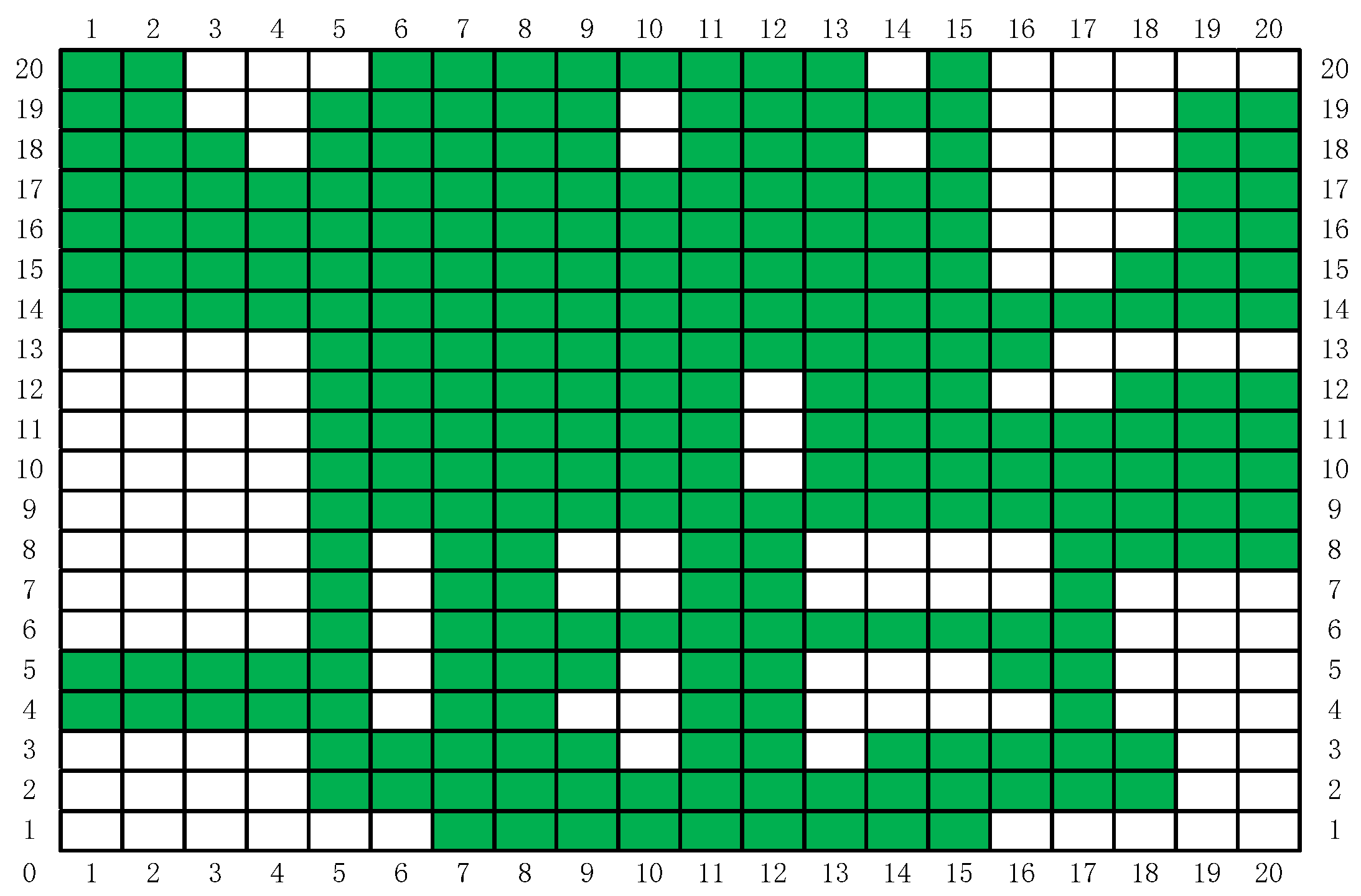
3.2.1. Path Planning Model Establishment
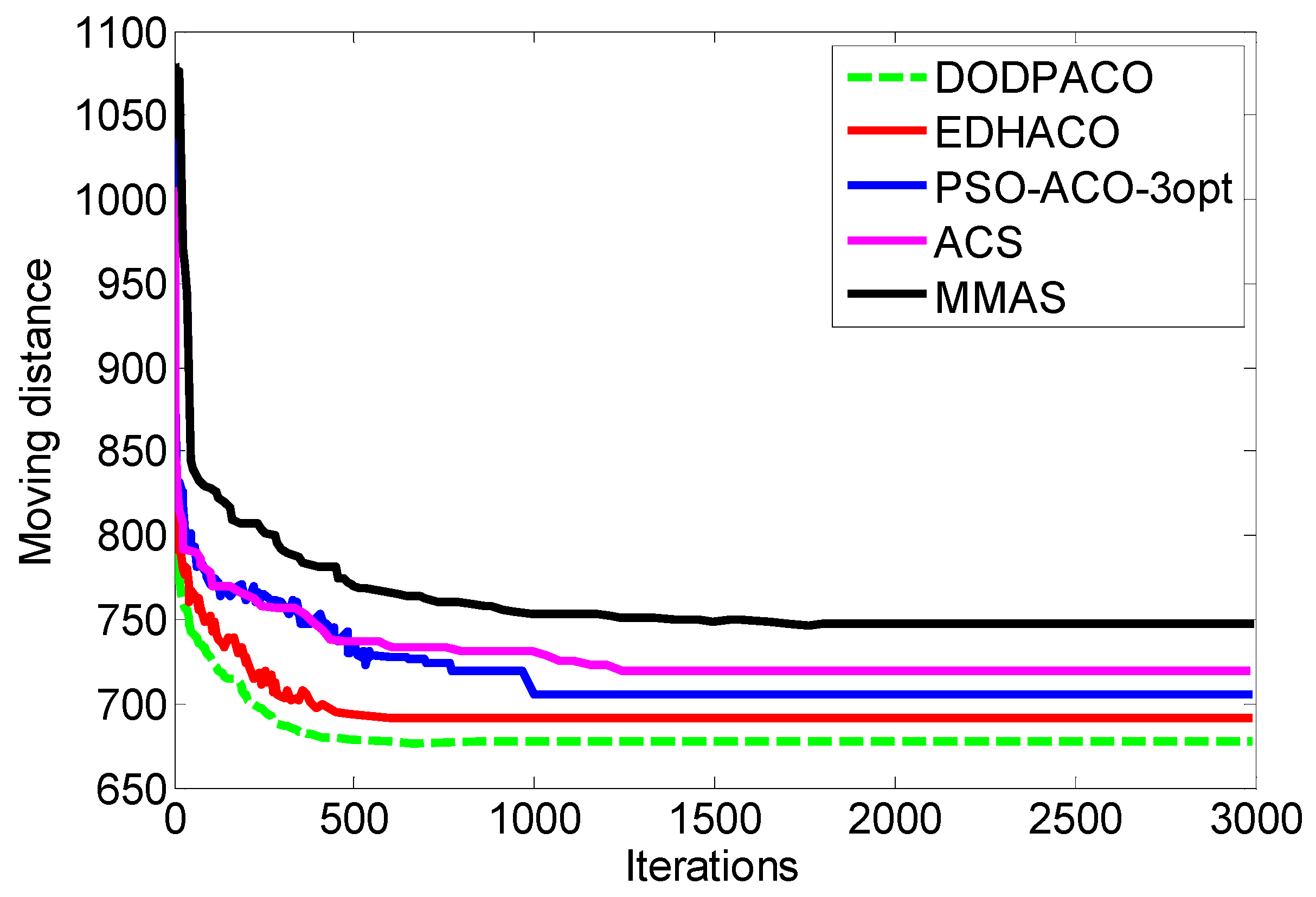
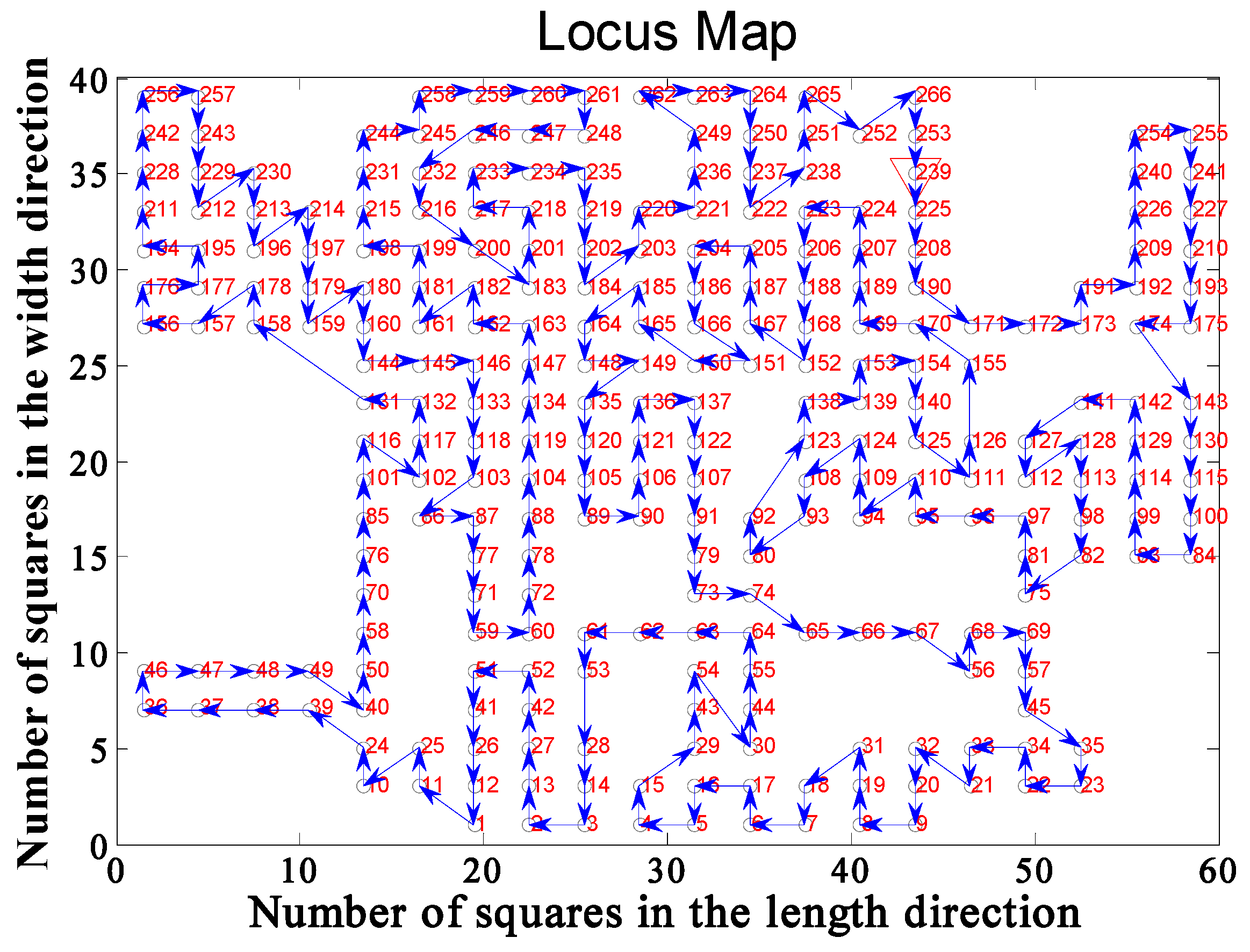
3.2.2. Verification Experiments
3.2.3. Discussion
4. Conclusions
Author Contributions
Funding
Conflicts of Interest
References
- Dinh, D.H.; Chien, H.L.; Lee, Y.C. Maskless lithography based on digital micromirror device (DMD) and double sided microlens and spatial filter array. Opt. Laser Technol. 2019, 113, 407–415. [Google Scholar] [CrossRef]
- Matteo, A. E-beam lithography for micro-/nano fabrication. Biomicrofluidics 2010, 4, 26503. [Google Scholar]
- Bae, B.S.; Park, O.H.; Charters, R.; Luther-Davies, B.; Atkins, G.R. Direct laser writing of self-developed waveguides in benzyldimethylketal-doped sol-gel hybrid glass. J. Mater. Res. 2001, 16, 3184–3187. [Google Scholar] [CrossRef] [Green Version]
- Seo, J.H.; Park, J.H.; Kim, S.I.; Park, B.J.; Ma, Z.; Choi, J.; Ju, B.K. Nanopatterning by laser interference lithography: Applications to optical devices. J. Nanosci. Nanotechnol. 2014, 14, 1521–1532. [Google Scholar] [CrossRef] [PubMed]
- Baglin, J.E.E. Ion beam nanoscale fabrication and lithography-A review. Appl. Surf. Sci. 2012, 258, 4103–4111. [Google Scholar] [CrossRef]
- Xiong, Z.; Liu, H.; Tan, X.; Lu, Z.; Li, C.; Song, L.; Wang, Z. Diffraction analysis of digital micromirror device in maskless photolithography system. J. Micro-Nanolith. MEM. 2014, 13, 43016. [Google Scholar] [CrossRef]
- Guo, X.; Du, J.; Guo, Y.; Du, C.; Cui, Z.; Yao, J. Simulation of DOE fabrication using DMD-based gray-tone lithography. Microelectron. Eng. 2006, 83, 1012–1016. [Google Scholar] [CrossRef]
- Chan, K.F.; Ren, Y. High-resolution maskless lithography. J. Microlith. Microfab. 2003, 2, 331–339. [Google Scholar] [CrossRef]
- Chen, R.; Liu, H.; Zhang, H.; Zhang, W.; Xu, J.; Xu, W.; Li, J. Edge smoothness enhancement in DMD scanning lithography system based on a wobulation technique. Opt. Express 2017, 25, 21958–21968. [Google Scholar] [CrossRef] [PubMed]
- Li, Q.K.; Xiao, Y.; Liu, H.; Zhang, H.L.; Xu, J.; Li, J.H. Analysis and correction of the distortion error in a DMD based scanning lithography system. Opt. Commun. 2019, 434, 1–6. [Google Scholar] [CrossRef]
- Lake, J.H.; Cambron, S.D.; Walsh, K.M.; McNamara, S. Maskless grayscale lithography using a positive-tone photo definable polyimide for MEMS applications. J. Microelectromech. Syst. 2011, 20, 1483–1488. [Google Scholar] [CrossRef]
- Zhong, K.; Gao, Y.; Li, F.; Luo, N.; Zhang, W. Fabrication of continuous relief micro-optic elements using real-time maskless lithography technique based on DMD. Opt. Laser Technol. 2014, 56, 367–371. [Google Scholar] [CrossRef]
- Liu, J.; Liu, J.; Deng, Q.; Liu, X.; He, Y.; Tang, Y.; Hu, S. Dose-modulated maskless lithography for the efficient fabrication of compound eyes with enlarged field-of-view. IEEE Photonics J. 2019, 11, 2400110. [Google Scholar] [CrossRef]
- Song, S.H.; Kim, K.; Choi, S.E.; Han, S.; Lee, H.S.; Kwon, S.; Park, W. Fine-tuned grayscale optofluidic maskless lithography for three-dimensional freeform shape microstructure fabrication. Opt. Lett. 2014, 39, 5162–5165. [Google Scholar] [CrossRef]
- Waldbaur, A.; Waterkotte, B.; Schmitz, K.; Rapp, B.E. Maskless projection lithography for the fast and flexible generation of grayscale protein patterns. Small 2012, 8, 1–9. [Google Scholar] [CrossRef] [PubMed]
- Wang, Q.; Zheng, J.; Wang, K.; Gui, K.; Guo, H.; Zhuang, S. Parallel detection experiment of fluorescence confocal microscopy using DMD. Scanning 2016, 38, 234–239. [Google Scholar] [CrossRef]
- Rammohan, A.; Dwivedi, P.K.; Martinez-Duarte, R.; Katepalli, H.; Madou, M.J.; Sharma, A. One-step maskless grayscale lithography for the fabrication of 3-dimensional structures in SU-8. Sens. Actuators B Chem. 2011, 153, 125–134. [Google Scholar] [CrossRef]
- Hansotte, E.J.; Carignan, E.C.; Meisburger, W.D. High speed maskless lithography of printed circuit boards using digital micromirrors. In Emerging Digital Micromirror Device Based Systems and Applications III; International Society for Optics and Photonics: Bellingham, WA, USA, 2011; Volume 793207. [Google Scholar]
- Lee, J.; Lee, H.; Yang, J. A rasterization method for generating exposure pattern images with optical maskless lithography. J. Mech. Sci. Technol. 2018, 32, 2209–2218. [Google Scholar] [CrossRef]
- Ryoo, H.; Kang, D.W.; Hahn, J.W. Analysis of the line pattern width and exposure efficiency in maskless lithography using a digital micromirror device. Microelectron. Eng. 2011, 88, 3145–3149. [Google Scholar] [CrossRef]
- Ryoo, H.; Kang, D.W.; Hahn, J.W.; Song, Y.T. Experimental analysis of pattern line width in digital maskless lithography. J. Micro-Nanolith. MEM. 2012, 11, 23004. [Google Scholar] [CrossRef]
- Xiong, Z.; Liu, H.; Chen, R.; Xu, J.; Li, Q.; Li, J.; Zhang, W. Illumination uniformity improvement in digital micromirror device based scanning photolithography system. Opt. Express 2018, 26, 18597–18607. [Google Scholar] [CrossRef] [PubMed]
- Wei, X.; Han, L.; Hong, L. A modified ant colony algorithm for traveling salesman problem. Int. J. Comput. Commun. 2014, 9, 633–643. [Google Scholar] [CrossRef] [Green Version]
- Yang, F.; Wu, X. Trajectory Planning of Step-and-scan Lithography by Genetic Algorithm. Mech. Sci. Technol. Aerospace Eng. 2007, 26, 1545–1547. [Google Scholar]
- Kar, A.K. Bio inspired computing–a review of algorithms and scope of applications. Expert Syst. Appl. 2016, 59, 20–32. [Google Scholar] [CrossRef]
- Li, Y.; Mei, K.; Liu, Y. Improving the area efficiency of aco-based routing by directional pheromone in large-scale NoCs. Microprocess. Microsy 2016, 45, 81–94. [Google Scholar] [CrossRef]
- Dorigo, M.; Maniezzo, V.; Colorni, A. Ant System: An Autocatalytic Optimizing Process; Technology Report 91-016; Politecnico di Milano: Milan, Italy, 1991. [Google Scholar]
- Dorigo, M.; Colorni, A.; Maniezzo, V. Distributed Optimization by Ant Colonies; Elsevier Publishing: Amsterdam, The Netherlands, 1991; pp. 134–142. [Google Scholar]
- Dorigo, M.; Birattari, M.; Stützle, T. Ant Colony Optimization. IEEE Comput. Intell. Mag. 2006, 1, 28–39. [Google Scholar] [CrossRef]
- Dorigo, M.; Gambardella, L.M. Ant colony system: A cooperative learning approach to the traveling salesman problem. IEEE Trans. Evolut. Comput. 1997, 1, 53–66. [Google Scholar] [CrossRef] [Green Version]
- Zhang, H.; Han, J. Strategy of optimization in ant colony algorithm and simulation research. Comput. Eng. Appl. 2006, 25, 52–53. [Google Scholar]
- Deng, W.; Xu, J.; Zhao, H. An improved ant colony optimization algorithm based on hybrid strategies for scheduling problem. IEEE Access 2019, 7, 20281–20292. [Google Scholar] [CrossRef]
- Zhang, Y.; Le, J.; Liao, X.; Zheng, F.; Liu, K.; An, X. Multi-objective hydro-thermal-wind coordination scheduling integrated with large-scale electric vehicles using IMOPSO. Renew. Energy. 2018, 128, 91–107. [Google Scholar] [CrossRef]
- Chen, J.; You, X.M.; Liu, S.; Li, J. Entropy-Based Dynamic Heterogeneous Ant Colony Optimization. IEEE Access 2019, 7, 56317–56328. [Google Scholar] [CrossRef]
- Jia, Z.H.; Zhang, Y.L.; Leung JY, T.; Li, K. Bi-criteria ant colony optimization algorithm for minimizing makespan and energy consumption on parallel batch machines. Appl. Soft Comput. 2017, 55, 226–237. [Google Scholar] [CrossRef]
- Sun, X.; Zhang, K.; Ma, M.; Su, H. Multi-population ant colony algorithm for virtual machine deployment. IEEE Access 2017, 5, 27014–27022. [Google Scholar] [CrossRef]
- Guan, B.; Zhao, Y. Self-adjusting ant colony optimization based on information entropy for detecting epistatic interactions. Genes 2019, 10, 114. [Google Scholar] [CrossRef] [Green Version]
- Chen, E.; Liu, X. Multi-colony ant algorithm using both repulsive operator and pheromone crossover based on multi-optimum for tsp. In Proceedings of the 2009 International Conference on Business Intelligence and Financial Engineering, Beijing, China, 24–26 July 2009; pp. 69–73. [Google Scholar]
- Li, Q.; Ba, W.; Liu, J.L. Scheduling Based on An Ant Colony Algorithm with Crossover Operator. In Proceedings of the 3rd International Conference on Mechatronics and Control Engineering (ICMCE), Zhuhai, China, 27–28 August 2014; pp. 47–50. [Google Scholar]
- Mohsen, A.M. Annealing ant colony optimization with mutation operator for solving TSP. Comput. Intell. Neurosc. 2016, 2016, 8932896. [Google Scholar] [CrossRef]
- Kalayci, C.B.; Kaya, C. An ant colony system empowered variable neighborhood search algorithm for the vehicle routing problem with simultaneous pickup and delivery. Expert Syst. Appl. 2016, 66, 163–175. [Google Scholar] [CrossRef]
- Zhu, H.; You, X.; Liu, S. Multiple Ant Colony Optimization Based on Pearson Correlation Coefficient. IEEE Access 2019, 7, 61628–61638. [Google Scholar] [CrossRef]
- Mahi, M.; Baykan, Ö.K.; Kodaz, H. A new hybrid method based on particle swarm optimization, ant colony optimization and 3-opt algorithms for traveling salesman problem. Appl. Soft Comput. 2015, 30, 484–490. [Google Scholar] [CrossRef]
- Xu, M.; You, X.; Liu, S. A novel heuristic communication heterogeneous dual population ant colony optimization algorithm. IEEE Access 2017, 5, 18506–18515. [Google Scholar] [CrossRef]
- Zhang, H.; You, X. Multi-Population Ant Colony Optimization Algorithm Based on Congestion Factor and Co-Evolution Mechanism. IEEE Access 2019, 7, 158160–158169. [Google Scholar] [CrossRef]
- Ma, X.; Kato, Y.; Van Kempen, F.; Hirai, Y.; Tsuchiya, T.; Van Keulen, F.; Tabata, O. Experimental study of numerical optimization for 3-D microstructuring using DMD-based grayscale lithography. J. Microelectromech. Syst. 2015, 24, 1856–1867. [Google Scholar] [CrossRef]


| k | |||||||
|---|---|---|---|---|---|---|---|
| 1 | 5 | 8 | 0.80 | 0.70 | 3/n | 6/n | 0.28 |
| pr152 | d198 | TSP225 | a280 | lin318 | berlin52 | kroa100 | kroa200 |
|---|---|---|---|---|---|---|---|
| 95 | 140 | 155 | 175 | 220 | 126 | 134 | 182 |
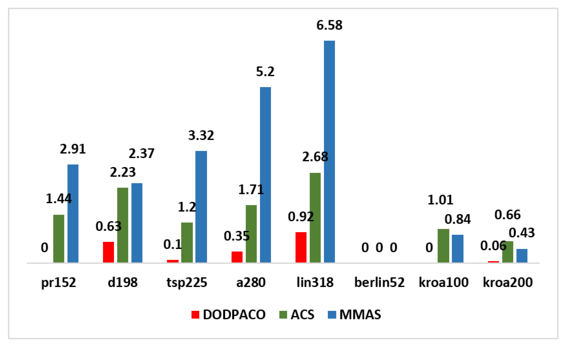
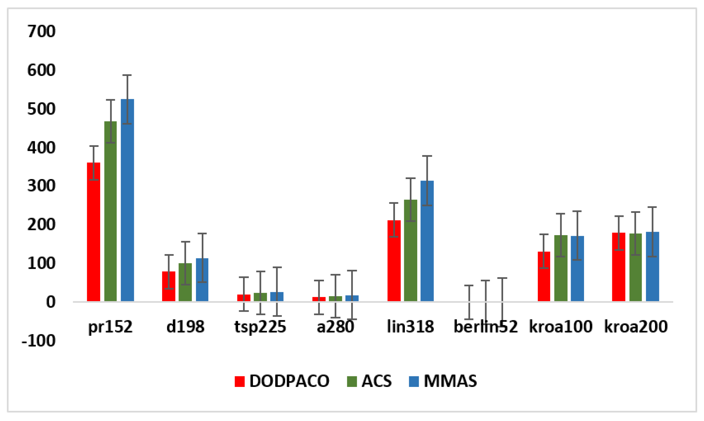
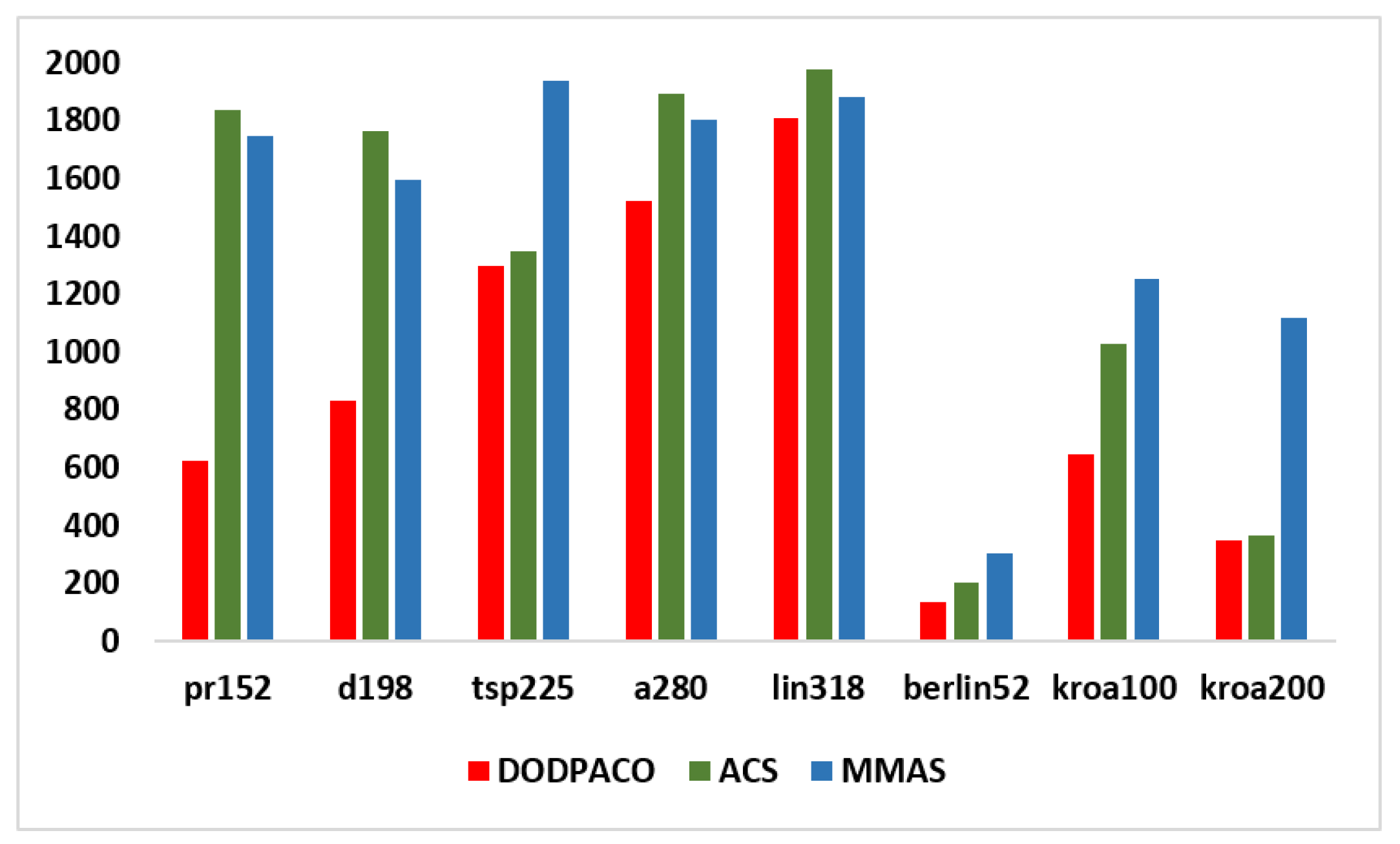
| Instance | Opt | Algorithms | Best | Mean | Error rate | Standard Deviation | Convergence |
|---|---|---|---|---|---|---|---|
| pr152 | 73,682 | DODPACO | 73,683 | 73,905 | 0.00 | 360 | 624 |
| ACS | 74,742 | 74,929 | 1.44 | 467 | 1838 | ||
| MMAS | 75,829 | 76,056 | 2.91 | 524 | 1745 | ||
| d198 | 15,780 | DODPACO | 15,790 | 15,896 | 0.63 | 79 | 832 |
| ACS | 16,132 | 16,172 | 2.23 | 101 | 1765 | ||
| MMAS | 16,154 | 16,20 | 2.37 | 114 | 1596 | ||
| TSP225 | 3916 | DODPACO | 3920 | 3963 | 0.10 | 21 | 1298 |
| ACS | 3963 | 3973 | 1.20 | 25 | 1349 | ||
| MMAS | 4046 | 4058 | 3.32 | 27 | 1940 | ||
| a280 | 2579 | DODPACO | 2588 | 2591 | 0.35 | 13 | 1521 |
| ACS | 2623 | 2630 | 1.71 | 16 | 1891 | ||
| MMAS | 2713 | 2721 | 5.20 | 19 | 1805 | ||
| lin318 | 42,029 | DODPACO | 42,416 | 42,458.42 | 0.92 | 212 | 1806 |
| ACS | 43,155 | 43,263 | 2.68 | 265 | 1979 | ||
| MMAS | 44,794 | 44,928 | 6.58 | 314 | 1881 | ||
| berlin52 | 7542 | DODPACO | 7542 | 7542 | 0 | 0 | 134 |
| ACS | 7542 | 7542 | 0 | 0 | 200 | ||
| MMAS | 7542 | 7542 | 0 | 0 | 304 | ||
| kroa100 | 26,524 | DODPACO | 21,282 | 21,286 | 0 | 132 | 645 |
| ACS | 26,793 | 26,938 | 1.01 | 174 | 1029 | ||
| MMAS | 26,746 | 26,562 | 0.84 | 172 | 1254 | ||
| kroa200 | 29,368 | DODPACO | 29,387 | 29,506 | 0.06 | 179 | 349 |
| ACS | 29,561 | 30,732 | 0.66 | 177 | 367 | ||
| MMAS | 29,495 | 30,435 | 0.43 | 182 | 1120 |
| Algorithms | Instance | pr152 | d198 | TSP225 | a280 | lin318 | berlin52 | kroa100 | kroa200 |
|---|---|---|---|---|---|---|---|---|---|
| Known Best Solution | 73,682 | 15,780 | 3916 | 2579 | 42,029 | 7542 | 21,282 | 29,368 | |
| PCCACO | best | / | 15,814 | 3937 | / | 42,461 | 7542 | 21,282 | 29,391 |
| mean | / | 16,463 | 3981 | / | 42,933 | 7542 | 21,383 | 29,485 | |
| EDHACO | best | 73,682 | / | / | / | 43,291 | / | 21,282 | 29,694 |
| mean | 74,251.6 | / | / | / | 43,926.3 | / | 21,355.13 | 30,391 | |
| ICMPACO | best | / | / | 4106 | / | / | 7548.6 | / | 31,267 |
| mean | / | / | 4214 | / | / | 7621.36 | / | 32,086 | |
| PSO-ACO-3opt | best | / | / | 4135 | / | / | 7542 | 21,301 | 29,468 |
| mean | / | / | 4250 | / | / | 7543.2 | 21,445.1 | 29,957 | |
| HHACO | best | / | / | 3998 | / | / | / | / | / |
| mean | / | / | 4113 | / | / | / | / | / | |
| CCMACO | best | / | / | 3926 | 2592 | 42,475 | / | 21,282 | 29,399 |
| mean | / | / | 4086.5 | 2682.6 | 42,682.7 | / | 21,488.3 | 29,834.8 | |
| Proposed Method DODPACO | best | 73,683 | 15,790 | 3920 | 2588 | 42,416 | 7542 | 21,282 | 29,387 |
| mean | 73,905 | 15,896 | 3963 | 2591 | 42,458 | 7542 | 21,286 | 29,356 |
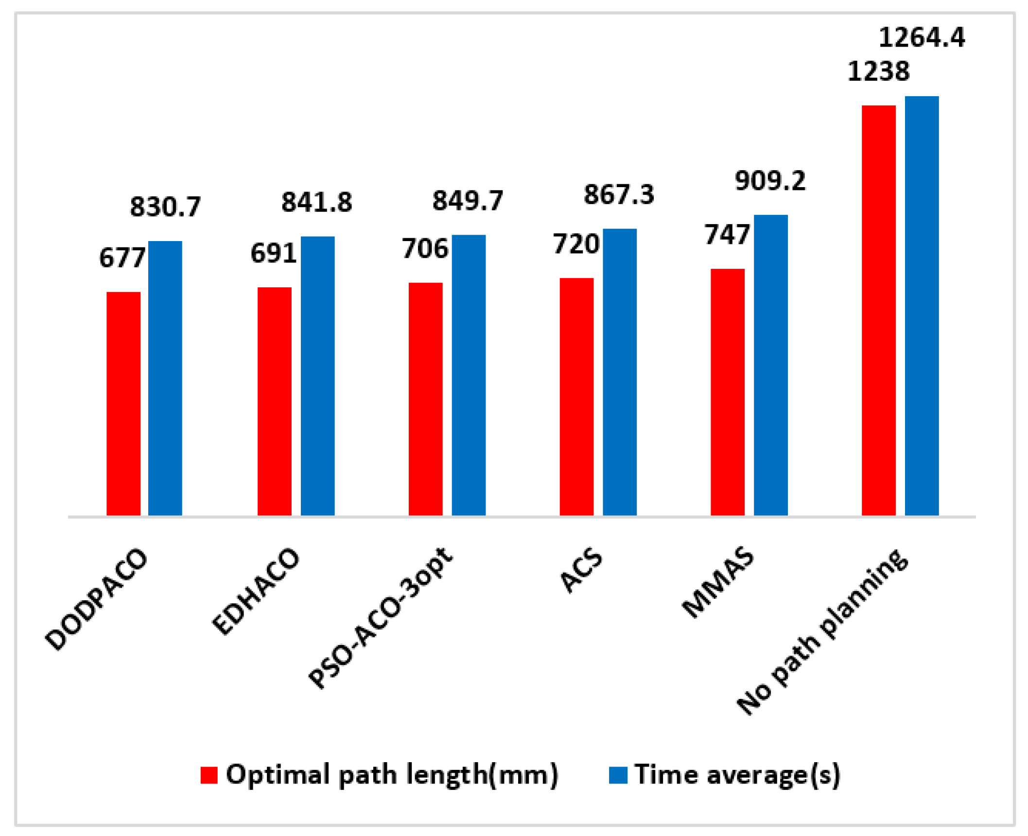
| Algorithms | DODPACO | EDHACO | PSO-ACO-3opt | ACS | MMAS | No Path Planning |
|---|---|---|---|---|---|---|
| Optimal path length (mm) | 677 | 691 | 706 | 720 | 747 | 1238 |
| Time average (s) | 830.7 | 841.8 | 849.7 | 867.3 | 909.2 | 1264.4 |
| Time savings compared with no-path planning (%) | 34.3 | 33.4 | 32.8 | 31.4 | 28.1 | 0 |
© 2020 by the authors. Licensee MDPI, Basel, Switzerland. This article is an open access article distributed under the terms and conditions of the Creative Commons Attribution (CC BY) license (http://creativecommons.org/licenses/by/4.0/).
Share and Cite
Wang, Y.; Han, T.; Jiang, X.; Yan, Y.; Liu, H. Path Planning of Pattern Transfer Based on Dual-Operator and a Dual-Population Ant Colony Algorithm for Digital Mask Projection Lithography. Entropy 2020, 22, 295. https://0-doi-org.brum.beds.ac.uk/10.3390/e22030295
Wang Y, Han T, Jiang X, Yan Y, Liu H. Path Planning of Pattern Transfer Based on Dual-Operator and a Dual-Population Ant Colony Algorithm for Digital Mask Projection Lithography. Entropy. 2020; 22(3):295. https://0-doi-org.brum.beds.ac.uk/10.3390/e22030295
Chicago/Turabian StyleWang, Yingzhi, Tailin Han, Xu Jiang, Yuhan Yan, and Hong Liu. 2020. "Path Planning of Pattern Transfer Based on Dual-Operator and a Dual-Population Ant Colony Algorithm for Digital Mask Projection Lithography" Entropy 22, no. 3: 295. https://0-doi-org.brum.beds.ac.uk/10.3390/e22030295