
Entanglement and Photon Anti-Bunching in Coupled Non-Degenerate Parametric Oscillators

1
Physics and Informatics Laboratories, NTT Research Inc., 940 Stewart Dr, Sunnyvale, CA 94085, USA
2
E. L. Ginzton Laboratory, Stanford University, Stanford, CA 94305, USA
*
Author to whom correspondence should be addressed.
Entropy 2021, 23(5), 624; https://0-doi-org.brum.beds.ac.uk/10.3390/e23050624
Submission received: 31 March 2021
/
Revised: 10 May 2021
/
Accepted: 13 May 2021
/
Published: 17 May 2021
(This article belongs to the Special Issue Quantum Measurement and Control in Quantum Machine Learning)
Abstract
:We analytically and numerically show that the Hillery-Zubairy’s entanglement criterion is satisfied both below and above the threshold of coupled non-degenerate optical parametric oscillators (NOPOs) with strong nonlinear gain saturation and dissipative linear coupling. We investigated two cases: for large pump mode dissipation, below-threshold entanglement is possible only when the parametric interaction has an enough detuning among the signal, idler, and pump photon modes. On the other hand, for a large dissipative coupling, below-threshold entanglement is possible even when there is no detuning in the parametric interaction. In both cases, a non-Gaussian state entanglement criterion is satisfied even at the threshold. Recent progress in nano-photonic devices might make it possible to experimentally demonstrate this phase transition in a coherent XY machine with quantum correlations.
1. Introduction
Networks of degenerate optical parametric oscillators (DOPOs), called coherent Ising machines (CIMs) [1,2,3,4,5,6,7,8,9,10,11,12,13], have been extensively studied from quantum optics and neural-network perspectives (for a recent review, see Ref. [14]). A DOPO network is constructed with a dissipative (Liouvillian) linear coupling rather than a conservative (Hamiltonian) coupling using either optical delay lines [2,5,6] or homodyne measurement feedback circuits [7,8,12]. The fundamental topics in quantum optics that can be studied with CIMs include Gaussian state entanglement [3,4], the Schrödinger cat state [10], and the entangled cat state [15]. Applications cover a broad spectrum, including spin-glass solvers [16,17], structure-based virtual screening for drug discovery [18], combinatorial optimization [12,19], compressed sensing [20], and fair sampling for deep machine learning [21].
The fundamental quantum resources of CIMs come from the phase-sensitive amplification/deamplification of two quadrature amplitudes in the DOPO [22]. Quantum correlation among DOPOs, evaluated by entanglement and quantum discord, reaches a maximum at the DOPO threshold and decreases below and above the threshold [23]. This quantum resource comes at the cost of limiting the spin-like degrees of freedom for computation and simulation. The in-phase quadrature amplitude (a canonical coordinate of a harmonic oscillator) takes either one of the bi-stable values above the threshold. We can relax this binary constraint using phase-insensitive oscillators such as lasers [24,25,26] or exciton-polariton condensates [27,28], in which the optical or polaritonic field can take a continuous phase above the threshold, so that an XY Hamiltonian (or Kuramoto model) can be naturally implemented instead of the Ising Hamiltonian. We call such a network as a coherent XY machine (CXM) in this paper. However, the bosonic fields in lasers and polariton condensates are thermal statistical mixture states below the threshold, while they approach coherent states far above the threshold [29]. The lack of non-classical states in lasers and polariton condensates seems to exclude the possibility of creating quantum correlations in a CXM based on such classical oscillators.
Non-degenerate optical parametric oscillators (NOPOs) have recently been used to construct a CXM [30]. One of the experimental advantages of an NOPO-based CXM is that we can easily transform a CIM to a CXM by introducing the frequency non-degeneracy between the signal and idler waves without changing the basic structure of the machine. An NOPO is a phase insensitive oscillator with a continuous phase degree of freedom, but its quantum statistical features are unique and distinct from standard lasers and polariton condensates. An NOPO below the threshold has a stronger gain saturation than a standard laser, so that a sub-Poissonian light or even a single photon state may be generated if the system parameters are chosen appropriately. This non-classical behavior below the threshold is analogous to those of a strongly coupled atom-cavity system [31,32] and coherently excited Raman three-level system with a large coupling and detuning [33]. On the other hand, an NOPO above the threshold can produce an amplitude squeezed state with a reduced amplitude fluctuation due to the strong gain saturation and diverging phase fluctuation due to a random walk diffusion process. This non-classical behavior above the threshold is analogous to those of pump-noise-suppressed lasers [34,35,36,37,38,39]. When such non-classical states of light are mixed by dissipative (Liouvillian) coupling, it is expected that the quantum correlations will form among the two NOPOs, just as in the case of two DOPOs in a CIM [3,4,23]. This would be another advantage of NOPO-based CXMs.
In this paper, we investigate the formation of entanglement in a CXM consisting of two NOPOs with a large parametric gain and show that entanglement is achieved below, above, and at the threshold. We use both analytical and numerical methods, although the analytical one is used to calculate the entanglement characteristics only far below and far above the threshold. Our analytical study on above-threshold CXMs, started with c-number stochastic differential equations (cSDEs) in the positive-P representation [40,41]. The numerical simulations were performed using both the quantum master equation (QME) in the photon number representation, and the wave function Monte Carlo (WFMC) method [42]. The paper is organized as follows. We introduce the model of CXM consisting of two NOPOs in Section 2. In Section 3, we investigate the case of a large dissipation in the pump mode and find that a large detuning of the parametric interaction is required to satisfy the entanglement criterion below the threshold. Next, in Section 4, we consider the case of a large dissipative coupling. We find that, below the threshold, entanglement is obtained even in the absence of detuning in the parametric interaction. Section 5 summarizes the paper. Appendix A shows the Fokker-Planck equation of the positive-P quasi-distribution function and derives the below-threshold characteristics of a single NOPO. Appendix B and Appendix C provide subsidiary information on the numerical and theoretical equations. Appendix D and Appendix E provide the detailed derivations of analytical results. Appendix F and Appendix G show the supplementary information about the entanglement criterion and the experimental NOPO [30].
2. Model
The density matrix equation of a single NOPO is written as
Here, , , and are pump, signal, and idler modes, respectively. These three photon modes have cavity frequencies and the linear dissipation rates . is the detuning of the parametric interaction. is the strength of the coherent excitation of the pump mode. is the strength of the parametric interaction. If the idler mode has a much larger dissipation than the other two photon modes (), the quantum master equation can be written as
Here G is the coefficient of the effective Raman interaction in Refs. [43,44,45], and K is the coefficient of the non-degenerate Kerr effect [46]. If , the Kerr coefficient is and the signal mode has a parametric gain . We define the maximum parametric gain as . For the detuned parametric interaction, the parametric gain is , and the Kerr coefficient is . We use the dimensionless detuning parameter to represent the normalized detuning. We also introduce the normalized excitation , where is the strength of the excitation at the oscillation threshold.
Let us consider a CXM consisting of two NOPOs (NOPO1 with and NOPO2 with ) coupled by a dissipative Liouvillian for two signal modes [3,4,47,48,49],
We will evaluate the entanglement between the two signal modes using one of the entanglement criteria in Ref. [50],
If this value is larger than zero, the two signal modes are entangled. Above the threshold, we assume the ferromagnetic configuration is created by the coupling Liouvillian (4). Using the fluctuation of positive-P amplitudes (introduced in Appendix A and Appendix B), the normalized is written as . Here, we assumed and that is real. Introducing the canonical coordinates and canonical momenta as and , this normalized entanglement criterion is written as
This criterion is equivalent to the Duan’s sufficient condition for entanglement (Theorem 1 of Ref. [51]). Moreover, criterion can detect an entanglement in a non-Gaussian state, for example, entanglement of a superposition of single photon states [52]. This criterion seems useful to detect non-Gaussian entanglement in the below-threshold CXM, since the similar model [33] realizes a single photon state.
3. Large Pump Dissipation Limit
3.1. Quantum Master Equation after the Elimination of the Pump Mode
In this section, we consider the large pump mode dissipation limit, where J. In this limit, the linear loss of the pump mode, due to the dissipation into the reservoir and spontaneous emission into the signal mode, is much larger than the linear loss of the signal mode. We will use the expansion of the density matrix with the complex-P representation [53,54] for the pump mode and photon number state representation for the signal mode:
Substituting this expansion into Equation (2), we can obtain a time development equation for .
Due to the linear dissipation of the signal mode (), components with photon number indices are excited by components with larger photon number indices . The parametric gain () introduces a contribution from components with smaller photon number indices . Other processes do not affect the photon number indices. Although the equation has drift terms for the pump amplitudes , the signal photon number indices do not change when components are derived using or . When is sufficiently large, the complex-P amplitude () at photon number indices (, ) rapidly converge to the steady-state value of the time-development equation . We can eliminate the pump mode amplitudes by writing , and integrating the complex-P amplitudes by . The density matrix components of the signal mode are,
Here , and . The denominators of these terms have higher dependence on the signal photon number than in Scully–Lamb’s theory [55]. In regard to the CXM consisting of two NOPOs, we can omit the subscript for the signal mode s, after eliminating the pump mode. The density matrix components of the two signal modes develop as,
3.2. Far-Below-Threshold Entanglement
From the above Equation (10), we will analytically derive the photon anti-bunching and entanglement characteristics far below the threshold (). In this limit, and are of order . Therefore, these contributions to on the right hand side of Equation (10) are much smaller than those of and J. However, the on the right hand side are not negligible. Although the on the right hand side do not contribute for small p, the non-degenerate Kerr coefficient K in the denominators of contributes to the characteristics far below the threshold. The signal photon number of the CXM is obtained from the equations of the two density-matrix components, , and .
From these equations, the mean signal photon number is . In the steady-state, this becomes
For a weak nonlinear gain saturation (), this value reaches one at . However, in general, is required for achieving , where stimulated emission becomes dominant over spontaneous emission. provides an amplitude correlation function between the two signal modes,
Next, we calculate the values of order from the equations of four components, , , and .
The second-order correlation function is obtained as . Its steady-state value is
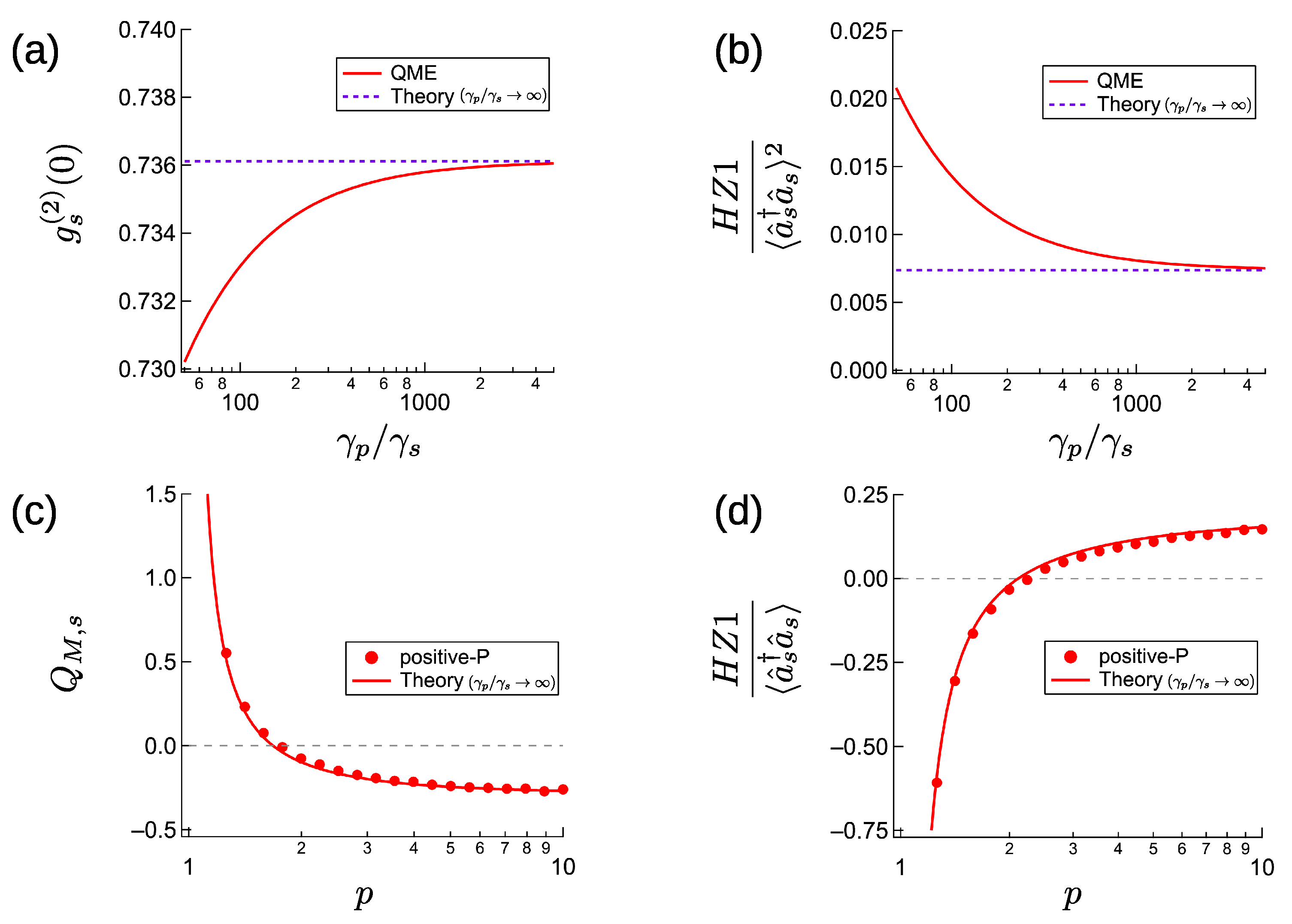
When the parametric coefficients are sufficiently small (), the signal modes are in blackbody radiation states with [29]. In the case of a large parametric gain (), however, the signal modes can have non-classical (photon anti-bunching) states with . In the single NOPO limit (), is obtained. This is identical to the limit of for a single NOPO, which is derived in Appendix A and shown in Equation (A15). This expression converges to a completely anti-bunching state in the limit [33]. In the limit, is , and it converges to in the large-K limit. This is larger than the minimum value for a single NOPO (). Hillery-Zubairy’s entanglement criterion (Equation (5)) for the two signal modes is obtained as , i.e.,
If this value is larger than zero, the two NOPOs are entangled far below the threshold. From the equation, is always negative if . To achieve entanglement, the detuning of the parametric interaction must be larger than the idler linewidth (). For below-threshold entanglement, a small ratio and large J are preferred.
The following is an example of a parameter set for below-threshold entanglement, , , and . These parameters give and . Therefore, the two NOPOs have anti-bunching states and are entangled. Figure 1a,b compares the analytically and numerically calculated and . The numerical results are obtained by time developing the quantum master Equation (3) from the vacuum state in accordance with the pump schedule . The values at are used as the approximate steady-state results for , and are plotted for various ratio. When becomes larger than by two orders of magnitude, and the below-threshold entanglement criterion converge to the analytical results that assume infinite .
3.3. Far-Above-Threshold Entanglement
Next, we analytically derive the above-threshold characteristics of the CXM by assuming a large pump dissipation and small parametric gain . We derive an analytical expression for the above-threshold fluctuations from the equations of positive-P representation [40,41]. For a single NOPO, the Fokker-Planck equation of the positive-P quasi-distribution function is derived in Appendix A. Here, are positive-P amplitudes for the pump (signal) mode. Using the Ito rule, the equivalent c-number stochastic differential equations are expressed as:
Here , and are independent complex Gaussian random numbers satisfying correlation functions, such as . reflects random spontaneous emission of signal photons. and contribute to the correlation between the pump and signal amplitudes. From Equations (23) and (24), the above-threshold pump photon number is identical to that of an NOPO without a Kerr term K [39]:
The above-threshold signal photon number is obtained from and
which is the steady-state mean of Equation (21), . Here, we have assumed that and . Using and , the steady-state signal photon number is obtained as
Here, is the normalized excitation modified by the detuning parameter in the parametric interaction. The steady-state pump amplitude is written as
By introducing the phase factor
the mean pump amplitude becomes .
Now let us introduce the small amplitude fluctuations in the pump and signal modes, and . The pump amplitude fluctuation is defined as the fluctuation after removing the phase factor denoted by .
The mean signal amplitude rotates with the frequency due to Kerr-nonlinearity. The signal amplitude fluctuation is defined as the fluctuation after removing this time-dependent phase factor,
These phase factors do not affect the products, and , appearing in the positive-P equations. The equations for small amplitude fluctuations are
Here, and . The time t is normalized so that is the unit time. The equivalent equations written with canonical coordinates and momenta are shown in Appendix C.
From these equations in the limit of , we can calculate the steady-state value of Mandel’s Q parameter [56] for a signal mode. It is defined as , where and . When is smaller than zero, the signal mode is in an amplitude squeezed state. From the calculation shown in the Appendix D,
is obtained. In the large excitation limit (), converges to a negative value . Therefore, an amplitude squeezed state is obtained even in a small-G NOPO. In the single NOPO limit (), . This value converges to for a large pump excitation, which is identical to the value obtained in Ref. [35]. In terms of the order , Mandel’s Q parameter is written as . Therefore, for the same p, detuning in the parametric interaction increases the amplitude squeezing. In the strong dissipative coupling limit, i.e., , the Mandel’s Q parameter is halved from that of the single NOPO limit.
The steady-state value of entanglement criterion is also obtained for large r, as
The detailed derivation is provided in Appendix D. Here, in the large excitation limit (), converges as . The coupling coefficient j must satisfy for entanglement far above the threshold. Therefore, detuning d is not preferred for satisfying above-threshold entanglement criterion, although must be satisfied for below-threshold entanglement.
The analytical and numerical Mandel’s Q parameter and entanglement criterion are compared in Figure 1c,d. Both results are obtained for and and plotted as the function of normalized excitation p. The analytical results assume that and . The numerical results were obtained by integrating the positive-Pc-number SDEs in Appendix B, for and . To obtain steady-state statistics from the positive-P calculation, we calculated a single trajectory, starting from with excitation depending on time as , and took the time average from to . The theoretical Mandel’s parameter from Equation (36) becomes negative at . The numerical values were slightly larger than the theoretical values due to the finite ratio. When , Equation (36) always gave at . Therefore, the non-degenerate Kerr effect causes amplitude squeezing for smaller p. Moreover, the theoretical from Equation (37) becomes positive for . The numerical values are slightly smaller than the analytical results due to the finite ratio. Above the threshold, the use of a small ratio helps to decrease the degrees of both amplitude squeezing and entanglement. This differs from the below threshold case, where using small ratio improves the anti-bunching and entanglement.
3.4. Numerical Results
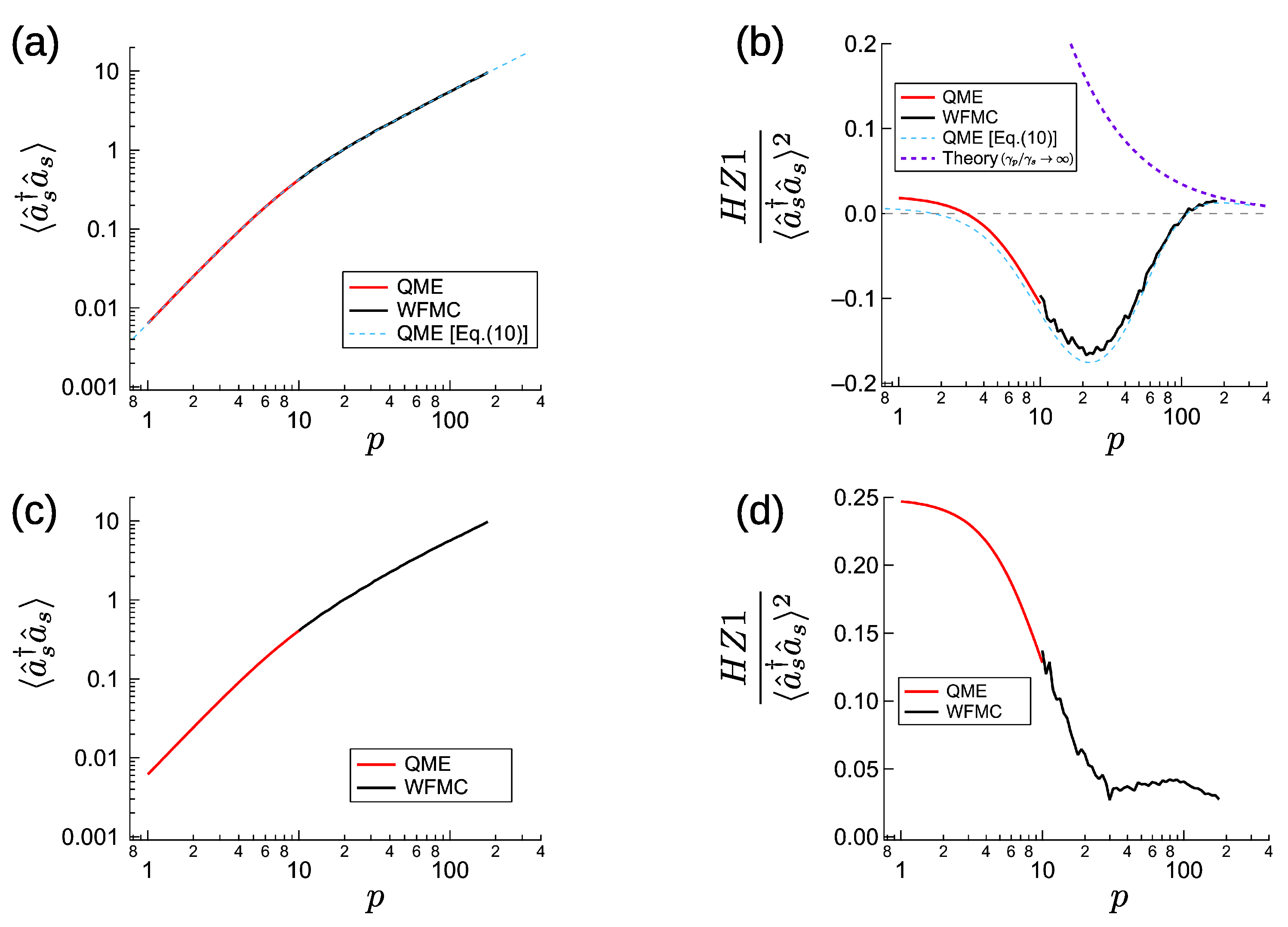
Here, we give the numerical simulation results as a function of normalized excitation p. The mean signal photon number and entanglement criterion are presented in Figure 2a,b for , , , and . For a small excitation p, we numerically calculated the quantum master equation (QME) in Equation (3) with a photon number space expansion. When the maximum pump photon number is and maximum signal photon number is in the expansion, the size of the density matrix and the calculation time are of order . This means that the calculation time increases rapidly for large p, where the mean signal photon number increases and we have to prepare a sufficiently larger satisfying . The maximum value of p calculated by QME was , where the mean signal photon number is , and we have used and . The method of the QME calculation is the same as for Figure 1a,b.
For a larger excitation p, we used Mølmer’s wave-function Monte Carlo (WFMC) calculation [42], whose calculation time is . In the WFMC calculation, time development started from the vacuum state with the excitation . A time average was taken from to , depending on the values of normalized excitation p. The calculation for small p with required more samples (longer period for time averaging) due to the slow convergence, although the size of the Hilbert space is smaller than that of the case of large p. The maximum p value calculated by WFMC was , where the mean signal photon number was , where we set and . The blue dashed line shows the results of the density matrix calculation with the pump mode eliminated in Equation (10). The calculation time of this method is , so we could use it to calculate even the above-threshold characteristics. We calculated the characteristics at with , where .
The numerical simulation indicated that the mean signal photon number does not show a rapid increase at the threshold. This behavior is known as a thresholdless lasing [57] and is obtained for a large nonlinear saturation coefficient. For an NOPO, different from a Scully–Lamb laser [55], the dependence of the signal photon number on p becomes smaller above the threshold. The below-threshold signal photon number is proportional to (Equation (13)), and the above-threshold signal photon number is proportional to p (Equation (27)). As a consequence of this behavior, a small stimulated emission below the threshold helps to reduce the signal photon number below the line. The Hillery-Zubairy’s entanglement criterion is satisfied far-below and far-above the threshold. This is an expected from the analytical results (K is much larger than G below the threshold, while above the threshold is satisfied). However, the small stimulated emission below the threshold gives a negative correction to . turned negative and reached a minimum value near the threshold (), where the signal photon number exceeds one. Far above the threshold converges to the theoretical values (purple dash line) obtained from dividing Equation (37) by Equation (27). Figure 2c,d presents the numerical simulation results for larger coupling coefficient (other parameters are the same as in Figure 2a,b). Equation (20) leads us to expected that a larger coupling coefficient increases the normalized value far below the threshold. Although a stimulated emission contributes negatively to the entanglement criterion, in a similar way to Figure 2b, always has a positive value even at the threshold. We thus obtained entanglement in below, above and at the threshold of the CXM, starting from a large pump mode dissipation.
4. Large Dissipative Coupling Limit
In the previous section, we showed that achieving entanglement at the threshold is not straightforward. The correction of the small stimulated emission to normalized is negative, and the entanglement criterion at the threshold can only be satisfied by increasing to the same order of . In Figure 1a,b, it can be seen that a large linewidth ratio () reduces the anti-bunching and entanglement. The theory for a large pump mode dissipation assumes the coupling coefficient J is much smaller than , which keeps J small and prevents quantum correlation between the two signal modes. Here, we consider another limit where J is sufficiently larger than the other parameters ().
4.1. Far-Below-Threshold Entanglement
First, we will consider the quantum statistics far below the threshold. Appendix A describes the procedure for deriving quantum statistics for a single NOPO far below the threshold. Briefly, this procedure starts from the truncated Fokker-Planck equation (Equation (A3)) in the positive-P representation, after the stimulated emission and Kerr non-linearity terms removed (which we write as ). We integrate the Fokker-Planck equation to obtain the time development equations of mean amplitude products and use them to derive the steady-state photon number and correlation functions. For a CXM, we start from the following Fokker-Planck equation,
Some of the steady-state results obtained from this Fokker-Planck equation are similar to, or even identical to the results for a single NOPO in Appendix A. Even with the large coupling of a signal mode, the pump amplitudes satisfy , which is identical to those of a single NOPO. However, as , the signal photon number becomes one half of that of a single NOPO . This is the same as the limit of Equation (13) obtained for large pump mode dissipation, and is also identical to the same limit of the two signal amplitudes’ correlation in Equation (14). We assume that such amplitude products connected by J, i.e., , to any replacement of and , have the same value in the zeroth order of .
The details of the derivation of are shown in Appendix E. In the large-J limit, the below-threshold second-order correlation function can be written as,
In the limit , this value converges to . This is different from the limit of Equation (19). If we start from large dissipative coupling , the anti-bunching state is obtained with large non-degenerate Kerr coefficient K. From Equation (39), the below-threshold entanglement criterion obeys as . The normalized with no detuning in the parametric interaction () is
This equation shows that the far-below-threshold entanglement criterion is satisfied even with . When , it is satisfied for .
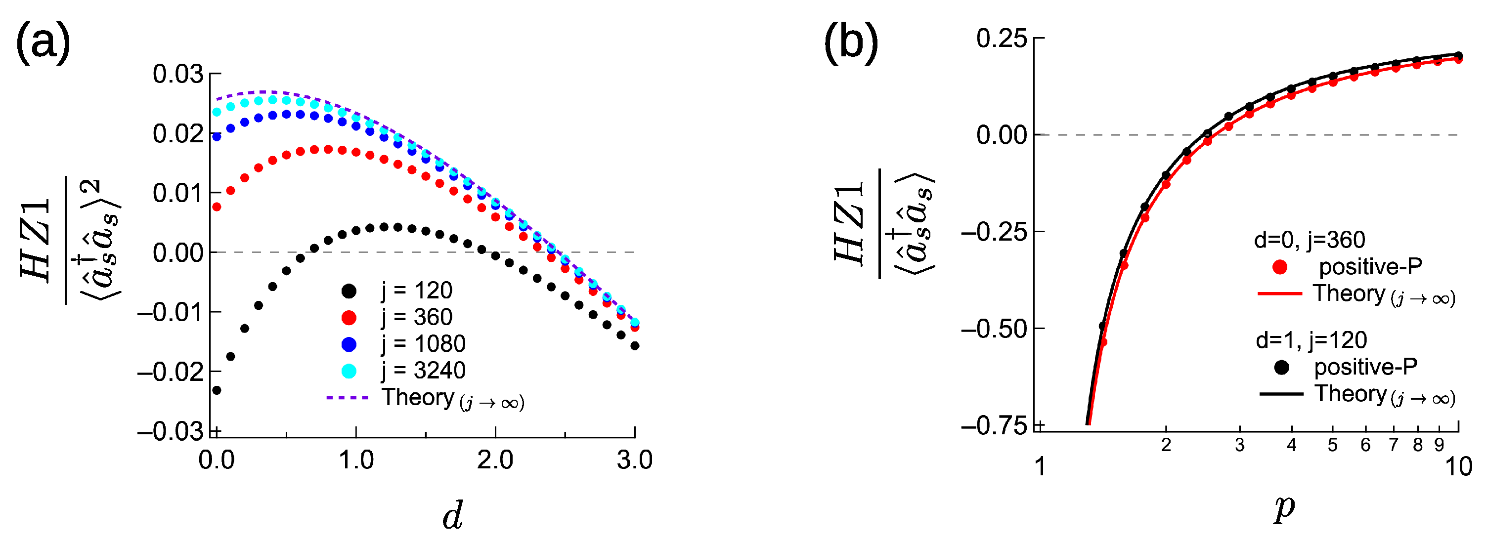
Figure 3a compares the normalized entanglement criterion obtained from the quantum master Equation (3) and the theory in the limit ( with Equation (39)). We set the linewidth ratio to 4 and the maximum parametric gain to 40 and investigate the impact of normalized detuning d in the parametric interaction. With detuning, the parametric gain becomes and the non-degenerate Kerr effect is . The numerical methods are the same as in Figure 1b. The numerical results with the largest j () have almost the same values as those in the theory assuming . Even in the limit, normalized slightly increases for a small detuning d. As d increases, K decreases as and gets closer to , where below-threshold entanglement is impossible. When , entanglement criterion is satisfied for . However, when , the entanglement criterion is not satisfied with zero detuning, although becomes positive with a non-zero detuning parameter.
4.2. Far-Above-Threshold Entanglement
Next, we derive the far-above-threshold entanglement in the limit . First of all, we will consider a single NOPO. From the cSDEs in Equations (32) and (33), we obtain the equations of the pump amplitude fluctuations, and . The equations in this representation are shown in Appendix C. The mean fluctuation products are
These pump amplitude fluctuations are excited by two fluctuation correlations, , and , where is the amplitude fluctuation of the signal mode. We introduce the normalized amplitude correlations,
The steady-state pump amplitude fluctuations in terms of A and B are
Next, we obtain the time development equations of , and .
is obtained from the steady state of Equation (51). Substituting Equations (46) and (48) into Equations (49) and (50), we obtain the steady-state signal amplitude fluctuation,
Here,
This fluctuation theory for a single NOPO is sufficient for calculating the normalized in a CXM in the limit. above the threshold obeys Equation (6) and includes a contributions from canonical momenta. However, for canonical momenta of signal modes, the fluctuation products of the CXM obey
The steady-state difference of these two fluctuation values is
which converges to zero in the large j limit. The sum appearing in the is the same as of a single NOPO shown in Equation (52). Finally, the normalized in the limit is
Mandel’s Q parameter for the signal mode is the same as in the limit. If we take the limit in Equation (57), the normalized entanglement criterion converges to , which is the same as the limit of the theory with a large pump dissipation (Equation (37)). This independence of the order of taking limits does not apply below the threshold. The correction to is negative: . Therefore, above-threshold entanglement is more easily obtained with large r (see Figure 1d).
We performed a numerical simulation using a positive-P equations in Appendix B. From Figure 3a with , we chose two sets of parameters: and . Below-threshold entanglement was achieved with these parameters, when we set a large parametric gain . Here, to check the far-above threshold entanglement, we performed the positive-P calculation for , with the same method as Figure 1d. The results are shown in Figure 3b. The numerical results fit the analytical ones (Equation (57)), which assume the limit. For , the numerical values are slightly smaller than the theoretical values, because the correction of reduces , as shown in Equation (37). Nevertheless, the values of normalized for are larger than for , because, as discussed in relation to Figure 1c, the correction makes it easier for an above-threshold NOPO to have a non-classical state.
4.3. Numerical Results
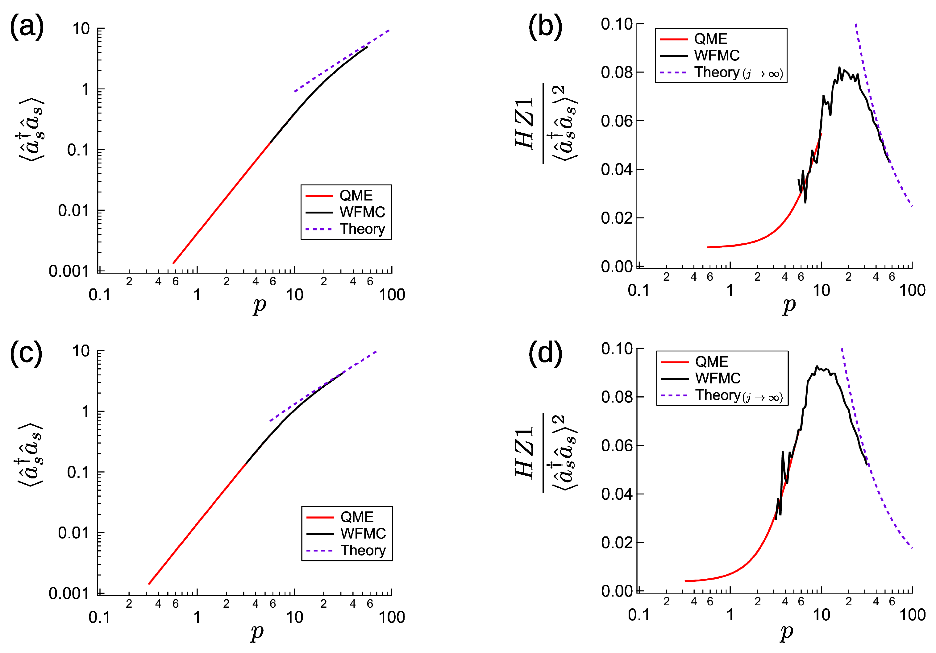
Here, we present the numerical simulation results as a function of normalized excitation p, for , and . The mean signal photon number and normalized are shown in Figure 4a,b. The numerical results are obtained by solving the QME (3) for small-p, and by performing a WFMC calculation [42] for large-p. The Methods are the same as those used to calculate the results shown in Figure 2, but for WFMC, the time average was taken from to depending on the excitation p. For the smallest p (∼5.6), time average was taken from to because of the slow convergence. For the maximum for WFMC, where the mean signal photon number is , we used a photon number space with and and took the time average from to . The purple dashed lines far-above the threshold are plots of Equation (27), or Equation (57) divided by Equation (27). The numerical results converge to the theoretical values far-above the threshold. The entanglement criterion is satisfied below and above the threshold, although the nonlinear Kerr effect is absent (). In contrast to Figure 2b,d, a small stimulated emission gave a positive correction to the normalized entanglement criterion . Because of this correction, the entanglement criterion is satisfied, even at the threshold. Next, we present the numerical simulation results for . As shown in Figure 4c,d, for the maximum p value (∼32) the mean signal photon number was . We used and for calculating this value. As with Figure 4b, stimulated emission gives a positive correction to the normalized value, which also results in entanglement at the threshold. As expected from Figure 3b, the peak value of the normalized is slightly larger than in Figure 4b.
5. Summary
We showed that Hillery-Zubairy’s entanglement criterion is satisfied in coherent XY machines, below, above, and even at the threshold of a CXM consisting of two highly non-Gaussian -NOPOs. We investigated two limits: (1) the pump mode has much larger dissipation than the signal mode, and (2) the dissipative coupling coefficient is much larger than the other parameters. In the first limit, below-threshold entanglement is possible only when the parametric coupling is detuned. In the second limit, below-threshold entanglement was obtained even when the parametric coupling is not detuned. In the first limit, although detuning of the parametric interaction is necessary to achieve below-threshold entanglement, it prevents above-threshold entanglement if J is comparable to . Moreover, the normalized entanglement criterion is decreased by a small stimulated emission, while in the second limit, the same value increased. The experimentally required for at-threshold entanglement is smaller for the second limit than the first. From these considerations, the second case with large dissipative coupling seems to be a more effective way to achieve entanglement at the threshold. For a more detailed study, other entanglement criteria should be discussed (In Appendix F, we discussed the Simon’s necessary and sufficient criterion for Gaussian state entanglement [58]). For obtaining entanglement at the threshold, the small stimulated emission correction to below-threshold , would be important. By further increasing G and K from the values we used in this paper, quantum state production in quantum spin model [59] would be possible in a CXM.
A large parametric interaction, , has been experimentally confirmed in a second-order nonlinear () rib-waveguide-based microring resonator [60]. The theoretical model studied in this paper could be realized by stimulated Raman scattering of traveling-wave modes in a silicon rib-waveguide [61], or standing-wave modes in silicon photonic crystal nanocavities [62,63], coupled via low-Q cavity mode [64]. For traveling wave model, the pulse period must be longer than the phonon lifetime to avoid unintentional correlation. In the standing-wave model, the parametric gain normalized by linear dissipation is calculated as [62]. Here, c is the speed of light in vaccum, is the quality factor of the signal cavity mode, is the coefficient of Raman amplification, is the relative dielectric coefficient of the material, and is the volume of the cavity (we used [65], and [62] for silicon photonic crystal nanocavity). The cavity quality factor must be as large as to achieve below-threshold entanglement. This is only an order of magnitude larger than the numerically achieved Q factor [66]. The hyper-parametric oscillation which enabled the CXM with third-order () nonlinearity [30] can have similar characteristics in terms of below-threshold anti-bunching or above-threshold amplitude squeezing (Appendix G). The CXMs of NOPOs seem to realize entanglement due to these non-classical characteristics.
Author Contributions
Formal analysis, Y.I.; Supervision, Y.Y. All authors have read and agreed to the published version of the manuscript.
Funding
This research received no external funding.
Conflicts of Interest
The authors declare no conflict of interest.
Appendix A. Fokker-Planck Equation and Far-Below Threshold Characteristics of Single NOPO
Here, we derive the below-threshold characteristics of a single NOPO using the positive-P Fokker-Planck equation. The positive-P distribution function is defined for a bosonic mode as [40,41],
For a single NOPO obeying Equation (2), the motion of the positive-P amplitudes, for the pump mode () and for the signal mode (), depends on the Fokker-Planck equation of the quasi-distribution function .
Next, we derive the far below-threshold characteristics (). Assuming small signal photon number (), we remove terms representing stimulated emission from the pump mode to the signal mode, and terms representing Kerr nonlinearity. After these terms have been removed, the Fokker-Planck equation of becomes
From this truncated Fokker-Planck equation, the mean of pump amplitude
(= develops as
The steady-state mean pump amplitude is written as
The time-development of higher order moments for the pump mode is obtained as,
Here, we neglect terms with a negative exponent in the right hand side. Far below the threshold, these moments in the steady state can be simply written as a product of steady-state mean pump amplitudes .
Next, the mean signal photon number develops as
The steady-state signal photon number is written as
Next, we consider higher-order moments containing signal mode amplitudes. To obtain the second-order correlation function of the signal mode , we derive the time development of from Equation (A3),
In the steady-state, the second order correlation function is
Here, is the correlation between the pump photon number and signal photon number. This photon number correlation develops as
The steady-state correlation function is
Here, is the correlation function between pump amplitude and signal photon number. This correlation is written as,
In the steady-state, we achieve.
The second-order correlation function of the signal mode of a below-threshold single NOPO is written as
This value is 2 for small [29], and it converges to zero in the large-K limit [33]. Even when (no detuning in the parametric interaction), a single NOPO can have an anti-bunching state () for large G. However, the minimum value is , instead of zero as obtained from the detuned parametric interaction.
Appendix B. Positive-P Equations for Numerical Calculation
The Fokker-Planck equation of the positive-P distribution function (Equation (A2)) has only first- and second-order derivatives of the positive-P amplitudes. Therefore, the Fokker-Planck equation of is rewritten as c-number stochastic differential equations (cSDEs) of the complex amplitudes (). For one Fokker-Planck equation, there can be multiple cSDEs with different coefficients of random numbers [41]. We used Equations (21)–(24) to derive the above-threshold fluctuation characteristics. In the numerical calculations to test the above-threshold characteritics, instead, we used the following equations of positive-P amplitudes,
These equations have two complex random numbers per NOPO, instead of three complex random numbers in Equations (21)–(24). In the CXM consisting of two NOPOs (Equation (3)), the equations of the signal amplitudes have additional terms due to the dissipative coupling Liouvillian, i.e., , , , and . The numerical results of the positive-P calculations are shown in Figure 1c,d and Figure 3b. These results are calculated for a small ratio. However, the positive-P calculation becomes unstable for a large ratio as shown in Figure 2 and Figure 4, although a large is essential for obtaining below-threshold entanglement. We used QME or WFMC to calculate the characteritics for a large parametric gain.
Appendix C. On the Fluctuations of Above-Threshold NOPO
Here, we summarize the different representation of above-threshold fluctuations of a single NOPO. After removing the phase factors from Equations (30) and (31), the equations of positive-P amplitudes become Equations (32)–(35). Here, we rewrite these equations with , and ,
Here, is a complex random number satisfying . are real random numbers satisfying . is the phase factor of the pump mode defined in Equation (29). It satisfies , and . These equations can also be written as , and .
Appendix D. Details of Above-Threshold Theory in the Large Pump Mode Dissipation Limit
In this appendix, we derive the above-threshold theory of CXM in the large pump mode dissipation limit. Assuming large , we can eliminate the pump mode and obtain the equations of signal-mode amplitude fluctuations from Equations (32)–(35), as
Here, and are independent real Gaussian noise satisfying and .
Using these equations, we will consider an CXM consisting of two NOPOs. Defining the coefficients, , , and , the fluctuations of the canonical coordinates obey,
where . Assuming a Gaussian state, the Mandel’s Q parameter is obtained as (shown in Equation (36)).
Next, we calculate the above-threshold values of Hillery-Zubairy’s entanglement criterion following Equation (6). The first two terms related to are obtained as . The mean fluctuation of diverges above the threshold of the NOPO. We can use a small lasing linewidth parameter to produce a finite fluctuation,
The contains the difference of these values, which is independent of small ,
Next, we consider the mean products of the and amplitudes, appearing in Equation (A30):
Since , the steady-state difference of these values is
Finally, the normalized criterion is obtained as Equation (37).
Appendix E. Details of Below-Threshold Theory in the Large Dissipative Coupling Limit
In this Appendix, we derive the second order correlation function for below-threshold CXM in the large dissipative coupling limit, using the assumption that values coupled by J have the same value in the large J limit. and the three values coupled to it via J obey,
There is no coupling coefficient J in the time-development equation of . Assuming that this weighted average is identical to in the zeroth order of , we obtain
From , the steady-state value of the second-order correlation function can be written as . Here, is the correlation function between the pump photon number and signal photon number.
Next, we calculate the correlation between the pump and signal photon numbers from the three following equations:
Moreover, there is no coupling coefficient J in the equation of . Assuming that this equation is identical to in the zeroth order of inverse coupling coefficient , the mean photon number product is,
From this equation, the steady-state pump-signal photon number correlation can be written as,
Here, we have used . is the correlation between the pump amplitude and the signal photon number.
To obtain the steady-state correlation function between the pump amplitude and the signal photon number, we derived the time development equations of four mean amplitude products,
The average of these four mean amplitude products obeys the equation without the coupling coefficient J. If we assume this average is identical to in the zeroth order of , we obtain
From this equation, the steady-state correlation between the pump amplitude and the signal photon number is
The second order correlation function of the far below-threshold large-J CXM is obtained in the form of Equation (39).
Appendix F. Simon’s Criterion for Above-Threshold Entanglement
For entanglement above the threshold, we can use Simon’s criterion [58], which is necessary and sufficient condition for entanglement when the states are Gaussian. When the above-threshold states of CXMs are treated as the Gaussian states with infinite fluctuations of canonical momenta, we can use this criterion. This criterion is described by a covariance matrix of two signal modes , where ( and are defined for positive-P amplitudes). If the minimum eigenvalue of (which we call ) is smaller than 1, for a partial-transposition matrix , and , the two signal modes are entangled [67].
From the equations in Appendix C (for , we add to the right hand side to avoid divergence), we obtain the steady-state values of 20 fluctuation products, , , , , , , , , , , and these between different NOPOs. From six values , , , , , and , we calculated the minimum symplectic eigenvalue of a partially transposed covariance matrix.
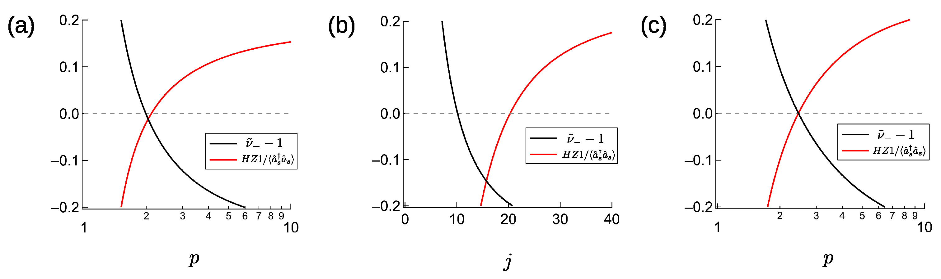
First, we study the limit of large pump mode dissipation. For , , , and , we plot the as a function of excitation p. The comparison with criterion is shown in Figure A1a. The entanglement criterion is satisfied for smaller 1.99) than the criterion . In the special case of , the Simon’s criterion is calculated as . Therefore, we need for entanglement in the limit, instead of larger 2) for . When , and , we show the j dependency of and the normalized in Figure A1b. The required j for above-threshold entanglement was also by a factor of 2 smaller for Simon’s criterion. Next, we show the results for large dissipative coupling. For , , , and , we plot the in Figure A1c. The Simon’s entanglement criterion is satisfied at the same 2.46) as the criterion.
Figure A1.
Comparison between Simon’s criterion () and for above-threshold CXM. (a,b) The case of large pump mode dissipation as a function of p or j. (c) The case of large dissipative coupling as a function of p.
Figure A1.
Comparison between Simon’s criterion () and for above-threshold CXM. (a,b) The case of large pump mode dissipation as a function of p or j. (c) The case of large dissipative coupling as a function of p.

Appendix G. Quantum Characteristics of Hyper-Parametric Oscillation
In this Appendix, we discuss the steady-state quantum statistics of hyper-parametric oscillation [30] in the limit of large idler mode dissipation and large parametric interaction. In this system, two degenerate pump photons are converted to a signal photon and an idler photon via a interaction. We use the Liouvillian derived for hyper-Raman scattering [68] with zero-temperature phonons. In this model of hyper-parametric oscillation, the density operator follows:
Here, the last term of Equation (2) are modified and was assumed. The excitation at the threshold of a hyper-parametric oscillation is written as , . As done in Equation (7), we expand the density operator with the complex-P representation for the pump mode and the photon number states representation for the signal mode: . We can obtain the time development equation for ,
When the signal photon number is fixed to , the pump mode has a coherent excitation, linear dissipation depending on , and two photon absorption depending on . When , the pump mode at each converges to a steady-state of the system of coherent excitation, linear dissipation, and two-photon absorption. The steady-state complex-P distribution function of such a system was derived in Ref. [40], . Here, and . We write the distribution function as . The hopping rate from to is proportional to , which is written as [40]
From the recursion relation of , the distribution of signal photon number is obtained as
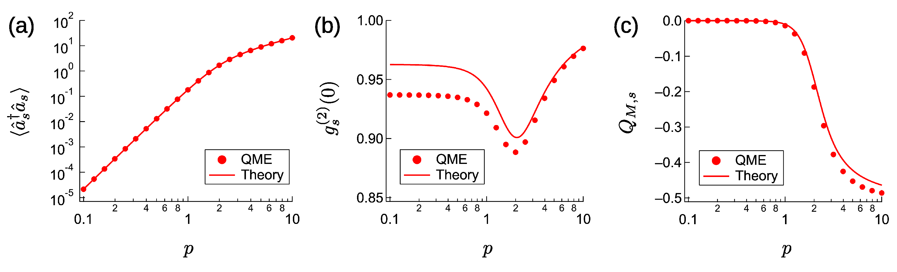
For , and , we show the comparison between numerical results of QME (calculated in the same methods as the main text) and the analytical results obtained by Equations (A52) and (A53). In Figure A2, two methods produced the same mean signal photon number, and the similar behavior of second order correlation function and Mandel’s Q parameter . Both methods show that the signal mode has a photon anti-bunching state below the threshold and an amplitude squeezed state above the threshold. In this special limit, is obtained far below the threshold, which is the same as -NOPO with (Equation (A15)). For the direct calculation of QME (Equation (A50)), the signal mode has a slightly smaller and , due to the finite and .
Figure A2.
Comparison between QME and analytical results for a hyper-parametric oscillator with . (a) Mean signal photon number. (b) The second order correlation function of the signal mode, . (c) Mandel’s Q parameter of the signal mode.
Figure A2.
Comparison between QME and analytical results for a hyper-parametric oscillator with . (a) Mean signal photon number. (b) The second order correlation function of the signal mode, . (c) Mandel’s Q parameter of the signal mode.

References
- Wang, Z.; Marandi, A.; Wen, K.; Byer, R.L.; Yamamoto, Y. Coherent Ising machine based on degenerate optical parametric oscillators. Phys. Rev. A 2013, 88, 063853. [Google Scholar] [CrossRef] [Green Version]
- Marandi, A.; Wang, Z.; Takata, K.; Byer, R.L.; Yamamoto, Y. Network of time-multiplexed optical parametric oscillators as a coherent Ising machine. Nat. Photon. 2014, 8, 937–942. [Google Scholar] [CrossRef] [Green Version]
- Takata, K.; Marandi, A.; Yamamoto, Y. Quantum correlation in degenerate optical parametric oscillators with mutual injections. Phys. Rev. A 2015, 92, 043821. [Google Scholar] [CrossRef] [Green Version]
- Maruo, D.; Utsunomiya, S.; Yamamoto, Y. Truncated Wigner theory of coherent Ising machines based on degenerate optical parametric oscillator network. Phys. Scr. 2016, 91, 083010. [Google Scholar] [CrossRef] [Green Version]
- Takata, K.; Marandi, A.; Hamerly, R.; Haribara, Y.; Maruo, D.; Tamate, S.; Sakaguchi, H.; Utsunomiya, S.; Yamamoto, Y. A 16-bit coherent Ising machine for one-dimensional ring and cubic graph problems. Sci. Rep. 2016, 6, 1–7. [Google Scholar] [CrossRef] [Green Version]
- Inagaki, T.; Inaba, K.; Hamerly, R.; Inoue, K.; Yamamoto, Y.; Takesue, H. Large-scale Ising spin network based on degenerate optical parametric oscillators. Nat. Photon. 2016, 10, 415–419. [Google Scholar] [CrossRef]
- McMahon, P.L.; Marandi, A.; Haribara, Y.; Hamerly, R.; Langrock, C.; Tamate, S.; Inagaki, T.; Takesue, H.; Utsunomiya, S.; Aihara, K.; et al. A Fully Program. 100-Spin Coherent Ising Mach. All- Connections. Science 2016, 354, 614–617. [Google Scholar] [CrossRef] [PubMed] [Green Version]
- Inagaki, T.; Haribara, Y.; Igarashi, K.; Sonobe, T.; Tamate, S.; Honjo, T.; Marandi, A.; McMahon, P.L.; Umeki, T.; Enbutsu, K.; et al. A Coherent Ising Mach. 2000-Node Optim. Problems. Science 2016, 354, 603–606. [Google Scholar] [CrossRef] [PubMed] [Green Version]
- Shoji, T.; Aihara, K.; Yamamoto, Y. Quantum model for coherent Ising machines: Stochastic differential equations with replicator dynamics. Phys. Rev. A 2017, 96, 053833. [Google Scholar] [CrossRef] [Green Version]
- Yamamura, A.; Aihara, K.; Yamamoto, Y. Quantum model for coherent Ising machines: Discrete-time measurement feedback formulation. Phys. Rev. A 2017, 96, 053834. [Google Scholar] [CrossRef] [Green Version]
- Yamamoto, Y.; Aihara, K.; Leleu, T.; Kawarabayashi, K.I.; Kako, S.; Fejer, M.; Inoue, K.; Takesue, H. Coherent Ising machines—Optical neural networks operating at the quantum limit. Npj Quantum Inf. 2017, 3, 1–15. [Google Scholar] [CrossRef] [Green Version]
- Hamerly, R.; Inagaki, T.; McMahon, P.L.; Venturelli, D.; Marandi, A.; Onodera, T.; Ng, E.; Langrock, C.; Inaba, K.; Honjo, T.; et al. Exp. Investig. Perform. Differ. Coherent Ising Mach. A Quantum Annealer. Sci. Adv. 2019, 5, eaau0823. [Google Scholar] [CrossRef] [PubMed] [Green Version]
- Kako, S.; Leleu, T.; Inui, Y.; Khoyratee, F.; Reifenstein, S.; Yamamoto, Y. Coherent Ising machines with error correction feedback. Adv. Quantum Technol. 2020, 3, 2000045. [Google Scholar] [CrossRef]
- Yamamoto, Y.; Leleu, T.; Ganguli, S.; Mabuchi, H. Coherent Ising machines—Quantum optics and neural network Perspectives. Appl. Phys. Lett. 2020, 117, 160501. [Google Scholar] [CrossRef]
- Zhou, Z.Y.; Gneiting, C.; You, J.Q.; Nori, F. Generating and detecting entangled cat states in dissipatively coupled degenerate optical parametric oscillators. arXiv 2021, arXiv:2103.16090. [Google Scholar]
- Leleu, T.; Yamamoto, Y.; Utsunomiya, S.; Aihara, K. Combinatorial optimization using dynamical phase transitions in driven-dissipative systems. Phys. Rev. E 2017, 95, 022118. [Google Scholar] [CrossRef]
- Leleu, T.; Yamamoto, Y.; McMahon, P.L.; Aihara, K. Destabilization of local minima in analog spin systems by correction of amplitude heterogeneity. Phys. Rev. Lett. 2019, 122, 040607. [Google Scholar] [CrossRef] [Green Version]
- Sakaguchi, H.; Ogata, K.; Isomura, T.; Utsunomiya, S.; Yamamoto, Y.; Aihara, K. Boltzmann sampling by degenerate optical parametric oscillator network for structure-based virtual screening. Entropy 2016, 18, 365. [Google Scholar] [CrossRef]
- Haribara, Y.; Utsunomiya, S.; Yamamoto, Y. Computational principle and performance evaluation of coherent Ising machine based on degenerate optical parametric oscillator network. Entropy 2016, 18, 151. [Google Scholar] [CrossRef] [Green Version]
- Aonishi, T.; Mimura, K.; Okada, M.; Yamamoto, Y. Statistical mechanics of CDMA multiuser detector implemented in coherent Ising machine. J. Appl. Phys. 2018, 124, 233102. [Google Scholar] [CrossRef] [Green Version]
- Ng, E.; Onodera, T.; Kako, S.; McMahon, P.L.; Mabuchi, H.; Yamamoto, Y. Efficient sampling of ground and low-energy Ising spin configurations with a coherent Ising machine. arXiv 2021, arXiv:2103.05629. [Google Scholar]
- Caves, C.M. Quantum limits on noise in linear amplifiers. Phys. Rev. D 1982, 26, 1817. [Google Scholar] [CrossRef]
- Inui, Y.; Yamamoto, Y. Entanglement and quantum discord in optically coupled coherent Ising machines. Phys. Rev. A 2020, 102, 062419. [Google Scholar] [CrossRef]
- Eckhouse, V.; Fridman, M.; Davidson, N.; Friesem, A.A. Loss enhanced phase locking in coupled oscillators. Phys. Rev. Lett. 2008, 100, 024102. [Google Scholar] [CrossRef] [PubMed]
- Nixon, M.; Ronen, E.; Friesem, A.A.; Davidson, N. Observing geometric frustration with thousands of coupled lasers. Phys. Rev. Lett. 2013, 110, 184102. [Google Scholar] [CrossRef] [PubMed]
- Pal, V.; Tradonsky, C.; Chriki, R.; Friesem, A.A.; Davidson, N. Observing dissipative topological defects with coupled lasers. Phys. Rev. Lett. 2017, 119, 013902. [Google Scholar] [CrossRef] [Green Version]
- Berloff, N.G.; Silva, M.; Kalinin, K.; Askitopoulos, A.; Töpfer, J.D.; Cilibrizzi, P.; Langbein, W.; Lagoudakis, P.G. Realizing the classical XY Hamiltonian in polariton simulators. Nat. Mater. 2017, 16, 1120–1126. [Google Scholar] [CrossRef]
- Kalinin, K.P.; Berloff, N.G. Networks of non-equilibrium condensates for global optimization. New J. Phys. 2018, 20, 113023. [Google Scholar] [CrossRef]
- Walls, D.F.; Milburn, G.J. Quantum Optics; Springer Science & Business Media: Berlin, Germany, 2007. [Google Scholar]
- Takeda, Y.; Tamate, S.; Yamamoto, Y.; Takesue, H.; Inagaki, T.; Utsunomiya, S. Boltzmann sampling for an XY model using a non-degenerate optical parametric oscillator network. Quantum Sci. Technol. 2017, 3, 014004. [Google Scholar] [CrossRef]
- Agarwal, G.S.; Gupta, S.D. Steady states in cavity QED due to incoherent pumping. Phys. Rev. A 1990, 42, 1737. [Google Scholar] [CrossRef]
- Gartner, P. Two-level laser: Analytical results and the laser transition. Phys. Rev. A 2011, 84, 053804. [Google Scholar] [CrossRef] [Green Version]
- Pellizzari, T.; Ritsch, H. Preparation of stationary Fock states in a one-atom Raman laser. Phys. Rev. Lett. 1994, 72, 3973. [Google Scholar] [CrossRef] [PubMed]
- Yamamoto, Y.; Machida, S.; Nilsson, O. Amplitude squeezing in a pump-noise-suppressed laser oscillator. Phys. Rev. A 1986, 34, 4025. [Google Scholar] [CrossRef] [PubMed]
- Ritsch, H.; Marte, M.A.M.; Zoller, P. Quantum noise reduction in Raman lasers. Europhys. Lett. 1992, 19, 7. [Google Scholar] [CrossRef]
- Gheri, K.M.; Walls, D.F. Sub-shot-noise lasers without inversion. Phys. Rev. Lett. 1992, 68, 3428. [Google Scholar] [CrossRef]
- Ralph, T.C. Squeezing from lasers. In Quantum Squeezing; Springer: Berlin/Heidelberg, Germany, 2004; pp. 141–170. [Google Scholar]
- Björk, G.; Yamamoto, Y. Phase correlation in nondegenerate parametric oscillators and amplifiers: Theory and applications. Phys. Rev. A 1988, 37, 1991. [Google Scholar] [CrossRef]
- Roos, P.A.; Murphy, S.K.; Meng, L.S.; Carlsten, J.L.; Ralph, T.C.; White, A.G.; Brasseur, J.K. Quantum theory of the far-off-resonance continuous-wave Raman laser: Heisenberg-Langevin approach. Phys. Rev. A 2003, 68, 013802. [Google Scholar] [CrossRef] [Green Version]
- Drummond, P.D.; Gardiner, C.W. Generalised P-representations in quantum optics. J. Phys. A 1980, 13, 2353. [Google Scholar] [CrossRef]
- Gilchrist, A.; Gardiner, C.W.; Drummond, P.D. Positive P representation: Application and validity. Phys. Rev. A 1997, 55, 3014. [Google Scholar] [CrossRef] [Green Version]
- Mølmer, K.; Castin, Y.; Dalibard, J. Monte Carlo wave-function method in quantum optics. JOSA B 1993, 10, 524–538. [Google Scholar] [CrossRef]
- Shen, Y.R. Quantum statistics of nonlinear optics. Phys. Rev. 1967, 155, 921. [Google Scholar] [CrossRef]
- Walls, D.F. A master equation approach to the Raman effect. J. Phys. A 1973, 6, 496. [Google Scholar] [CrossRef]
- McNeil, K.J.; Walls, D.F. A master equation approach to nonlinear optics. J. Phys. A 1974, 7, 617. [Google Scholar] [CrossRef]
- Holland, M.J.; Collett, M.J.; Walls, D.F.; Levenson, M.D. Nonideal quantum nondemolition measurements. Phys. Rev. A 1990, 42, 2995. [Google Scholar] [CrossRef] [PubMed]
- Koga, K.; Yamamoto, N. Dissipation-induced pure Gaussian state. Phys. Rev. A 2012, 85, 022103. [Google Scholar] [CrossRef] [Green Version]
- Goto, H. Quantum computation based on quantum adiabatic bifurcations of Kerr-nonlinear parametric oscillators. J. Phys. Soc. Jpn. 2019, 88, 061015. [Google Scholar] [CrossRef] [Green Version]
- Linowski, T.; Gneiting, C.; Rudnicki, Ł. Stabilizing entanglement in two-mode Gaussian states. Phys. Rev. A 2020, 102, 042405. [Google Scholar] [CrossRef]
- Hillery, M.; Zubairy, M.S. Entanglement conditions for two-mode states. Phys. Rev. Lett. 2006, 96, 050503. [Google Scholar] [CrossRef] [Green Version]
- Duan, L.M.; Giedke, G.; Cirac, J.I.; Zoller, P. Inseparability criterion for continuous variable systems. Phys. Rev. Lett. 2000, 84, 2722. [Google Scholar] [CrossRef] [Green Version]
- Hillery, M.; Zubairy, M.S. Entanglement conditions for two-mode states: Applications. Phys. Rev. A 2006, 74, 032333. [Google Scholar] [CrossRef] [Green Version]
- Drummond, P.D.; Walls, D.F. Quantum theory of optical bistability. I. Nonlinear polarisability model. J. Phys. A 1980, 13, 725. [Google Scholar] [CrossRef]
- Drummond, P.D.; Gardiner, C.W.; Walls, D.F. Quasiprobability methods for nonlinear chemical and optical systems. Phys. Rev. A 1981, 24, 914. [Google Scholar] [CrossRef]
- Scully, M.; Lamb, W.E., Jr. Quantum theory of an optical maser. Phys. Rev. Lett. 1966, 16, 853. [Google Scholar] [CrossRef]
- Mandel, L. Sub-Poissonian photon statistics in resonance fluorescence. Opt. Lett. 1979, 4, 205–207. [Google Scholar] [CrossRef] [PubMed]
- Björk, G.; Karlsson, A.; Yamamoto, Y. Definition of a laser threshold. Phys. Rev. A 1994, 50, 1675. [Google Scholar] [CrossRef]
- Simon, R. Peres-Horodecki separability criterion for continuous variable systems. Phys. Rev. Lett. 2000, 84, 2726. [Google Scholar] [CrossRef] [Green Version]
- Wang, X. Entanglement in the quantum Heisenberg XY model. Phys. Rev. A 2001, 64, 012313. [Google Scholar] [CrossRef] [Green Version]
- Lu, J.; Li, M.; Zou, C.L.; Al Sayem, A.; Tang, H.X. Toward 1% single-photon anharmonicity with periodically poled lithium niobate microring resonators. Optica 2020, 7, 1654–1659. [Google Scholar] [CrossRef]
- Boyraz, O.; Jalali, B. Demonstration of a silicon Raman laser. Opt. Express 2004, 12, 5269–5273. [Google Scholar] [CrossRef]
- Yang, X.; Wong, C.W. Coupled-mode theory for stimulated Raman scattering in high-Q/Vm silicon photonic band gap defect cavity lasers. Opt. Express 2007, 15, 4763–4780. [Google Scholar] [CrossRef] [Green Version]
- Takahashi, Y.; Inui, Y.; Chihara, M.; Asano, T.; Terawaki, R.; Noda, S. A micrometre-scale Raman silicon laser with a microwatt threshold. Nature 2013, 498, 470–474. [Google Scholar] [CrossRef] [PubMed]
- Sato, Y.; Tanaka, Y.; Upham, J.; Takahashi, Y.; Asano, T.; Noda, S. Strong coupling between distant photonic nanocavities and its dynamic control. Nat. Photon. 2012, 6, 56–61. [Google Scholar] [CrossRef]
- Dadap, J.I.; Espinola, R.L.; Osgood, R.M.; McNab, S.J.; Vlasov, Y.A. Spontaneous Raman scattering in ultrasmall silicon waveguides. Opt. Lett. 2004, 29, 2755–2757. [Google Scholar] [CrossRef] [PubMed]
- Asano, T.; Noda, S. Optimization of photonic crystal nanocavities based on deep learning. Opt. Express 2018, 26, 32704–32717. [Google Scholar] [CrossRef]
- Adesso, G.; Serafini, A.; Illuminati, F. Extremal entanglement and mixedness in continuous variable systems. Phys. Rev. A 2004, 70, 022318. [Google Scholar] [CrossRef] [Green Version]
- Simaan, H.D. A master equation approach to the hyper-Raman effect. J. Phys. A 1978, 11, 1799. [Google Scholar] [CrossRef]
Figure 1.
Below- and above-threshold characteristics of CXM with large pump dissipation for , . (a,b) Comparison of far-below-threshold theory () and quantum master equation with for . (c,d) Comparison of far-above-threshold theory () and positive-P numerical calculation with and .
Figure 1.
Below- and above-threshold characteristics of CXM with large pump dissipation for , . (a,b) Comparison of far-below-threshold theory () and quantum master equation with for . (c,d) Comparison of far-above-threshold theory () and positive-P numerical calculation with and .

Figure 2.
Numerically calculated steady-state of CXM with large pump dissipation, for , , . (a,b) Excitation dependent signal photon number and entanglement criterion for . (c,d) The same results for .
Figure 2.
Numerically calculated steady-state of CXM with large pump dissipation, for , , . (a,b) Excitation dependent signal photon number and entanglement criterion for . (c,d) The same results for .

Figure 3.
Far-below and far-above threshold characteristics of CXM with large dissipative coupling (), for . (a) Comparison of far-below threshold theory () and quantum master equation with , for . (b) Comparison of far-above threshold theory () and positive-P calculation with .
Figure 3.
Far-below and far-above threshold characteristics of CXM with large dissipative coupling (), for . (a) Comparison of far-below threshold theory () and quantum master equation with , for . (b) Comparison of far-above threshold theory () and positive-P calculation with .

Figure 4.
Numerical steady state of CXM with large dissipative coupling (), for , . (a,b) Excitation-dependent signal photon number and entanglement criterion for . (c,d) The same results for .
Figure 4.
Numerical steady state of CXM with large dissipative coupling (), for , . (a,b) Excitation-dependent signal photon number and entanglement criterion for . (c,d) The same results for .

Publisher’s Note: MDPI stays neutral with regard to jurisdictional claims in published maps and institutional affiliations. |
© 2021 by the authors. Licensee MDPI, Basel, Switzerland. This article is an open access article distributed under the terms and conditions of the Creative Commons Attribution (CC BY) license (https://creativecommons.org/licenses/by/4.0/).
Share and Cite
MDPI and ACS Style
Inui, Y.; Yamamoto, Y. Entanglement and Photon Anti-Bunching in Coupled Non-Degenerate Parametric Oscillators. Entropy 2021, 23, 624. https://0-doi-org.brum.beds.ac.uk/10.3390/e23050624
AMA Style
Inui Y, Yamamoto Y. Entanglement and Photon Anti-Bunching in Coupled Non-Degenerate Parametric Oscillators. Entropy. 2021; 23(5):624. https://0-doi-org.brum.beds.ac.uk/10.3390/e23050624
Chicago/Turabian StyleInui, Yoshitaka, and Yoshihisa Yamamoto. 2021. "Entanglement and Photon Anti-Bunching in Coupled Non-Degenerate Parametric Oscillators" Entropy 23, no. 5: 624. https://0-doi-org.brum.beds.ac.uk/10.3390/e23050624
Note that from the first issue of 2016, this journal uses article numbers instead of page numbers. See further details here.