
Unitary Evolution and Elements of Reality in Consecutive Quantum Measurements


1
Departmento de Química-Física, Universidad del País Vasco, UPV/EHU, 48940 Leioa, Spain
2
IKERBASQUE, Basque Foundation for Science, Plaza Euskadi 5, 48009 Bilbao, Spain
Entropy 2022, 24(7), 877; https://0-doi-org.brum.beds.ac.uk/10.3390/e24070877
Submission received: 9 June 2022
/
Revised: 16 June 2022
/
Accepted: 21 June 2022
/
Published: 26 June 2022
(This article belongs to the Special Issue The Philosophy of Quantum Physics)
Abstract
:Probabilities of the outcomes of consecutive quantum measurements can be obtained by construction probability amplitudes, thus implying the unitary evolution of the measured system, broken each time a measurement is made. In practice, the experimenter needs to know all past outcomes at the end of the experiment, and that requires the presence of probes carrying the corresponding records. With this in mind, we consider two different ways to extend the description of a quantum system beyond what is actually measured and recorded. One is to look for quantities whose values can be ascertained without altering the existing probabilities. Such “elements of reality” can be found, yet they suffer from the same drawback as their EPR counterparts. The probes designed to measure non-commuting operators frustrate each other if set up to work jointly, so no simultaneous values of such quantities can be established consistently. The other possibility is to investigate the system’s response to weekly coupled probes. Such weak probes are shown either to reduce to a small fraction the number of cases where the corresponding values are still accurately measured, or lead only to the evaluation of the system’s probability amplitudes, or their combinations. It is difficult, we conclude, to see in quantum mechanics anything other than a formalism for predicting the likelihoods of the recorded outcomes of actually performed observations.
PACS:
03.65.Ta; 03.65.AA; 03.65.UD1. Introduction
In [1], Feynman gave a brief yet surprisingly thorough description of quantum behaviour. Quantum systems are intrinsically stochastic, calculation of probabilities must rely on complex valued probability amplitudes, and it is unlikely that one will be able to get a further insight into the mechanism behind the formalism. One may ask two separate questions about the view expressed in [1]. Firstly, is it consistent? There have been recent suggestions [2] that quantum mechanics may be self-contradictory, and that its flaws can be detected from within the theory, i.e., by considering certain thought experiments. In [3], we have, argued that the proposed “contradictions” are easily resolved if Feynman’s description is adopted. Secondly, one can ask if the rules can be explained further? There have been proposals of “new physics” based on such concepts as time symmetry, weak measurements, and weak values (see [4,5,6], and Refs. therein). Recently, we have shown the weak values to be but Feynman’s probability amplitudes, or their combinations [7,8]. The ensuing paradoxes occur if the amplitudes are used inappropriately, e.g., as a proof of the system’s presence at a particular location [9], a practice known for quite some time to be unwise (see [10] and Ch. 6 pp. 144–145 of [11]). It is probably fair to say that Feynman’s conclusions have not been successfully challenged to date, and we will continue to rely on them in what follows.
The approach of [1] is particularly convenient for describing situations where several measurements are made one after another on the same quantum system. Such consecutive or sequential measurements have been studied by various authors over a number of years [12,13,14,15,16], and we will continue to study them here. The simplest case involves just two observations, of which the first prepares the measured system in a known state, and the second yields the value of the measured quantity “in that state.” Adding intermediate measurements between these two significantly changes the situation, as it brings in a new type of interference the measurements can now destroy. Below we will discuss two particular issues which arise in the analysis of such sequential measurements. One is the break down of the unitary evolution of the measured system, which occurs each time a measurement is made. Another is the possibility of extending the description of the system beyond what is actually being measured. This can be done, e.g., by looking for “elements of reality”, i.e., the properties or values which can be ascertained without changing anything else in the system’s evolution. This can also be done by studying a system’s response to weekly coupled inaccurate measuring devices. It is not our purpose here to dispute the findings made by the authors using alternative approaches (see, for example, [5]). Rather we we want to see how the above issues can be addressed in conventional quantum mechanics, as presented in [1].
The rest of the paper is organised as follows. In Section 2, we recall the basic rules and discuss the broken unitary evolution of the measured system, In Section 3, we note that, in order to be able to gather the statistics, the experimenter would need the records of the previous outcomes. The system’s broken evolution can then be traded for an unbroken unitary evolution of a composite {system + the probes which carry the records}. In Section 4, we discuss two different (and indeed well known) types of the probes. In Section 5, we discuss the quantities whose additional measurements would not alter the likelihoods of all other outcomes. However, like their EPR counterparts, these “elements of reality” cannot be observed simultaneously. In Section 6, we illustrate this on a simple two-level example. In Section 7, we look at what would happen in an attempt to measure two of such quantities jointly. Section 8 asks if something new can be learnt about the system by minimising the perturbation incurred by the probes. Section 9 contains a summary of our conclusions.
2. Feynman’s Rules of Quantum Motion: Broken Unitary Evolutions
Consider a system (S) with which the theory associates N-dimensional Hilbert space . The quantities to be measured at the times are represented by Hermitian operators acting in , each with distinct real valued eigenvalues
where , (, ) are the measurement bases, if , and 0 otherwise, and is the projector onto the eigen-subspace, corresponding to an eigenvalue . The first operator is assumed to have only non-degenerate eigenvalues, i.e., . This is needed to initialise the system, in order to proceed with the calculation.
The possible outcomes of the experiment are, therefore, the sequences of the observed values , and one wishes to predict the probabilities (frequencies) with which a particular real path would occur after many trials. Following [1], one can obtain these obtained by constructing first the system’s virtual paths , connecting the corresponding states in , and ascribing to each path a probability amplitude (we use )
where is the system’s evolution operator (the time ordered product is assumed if the system’s hamiltonian operators do not commute at different times, ). We will assume that all Hermitian operators can be measured in this way. We will also allow for all unitary evolutions, .
Combining the virtual paths according to the degeneracies of the intermediate eigenvalues , , yields elementary paths, endowed with both the amplitudes
and the probabilities,
We note that the amplitudes in Equation (3) depend only on the projectors in Equation (2), and not on the corresponding eigenvalues . To stress this, we are able to write
Finally, summing over the degeneracies of the last operator , yields the desired probabilities for the real paths,
Note that there is no interference between the paths leading to different (i.e., orthogonal) final states , even if they correspond to the same eigenvalue [1]. This is necessary, since an additional ()-nd measurement of an operator immediately after would destroy any interference between the paths ending in different s at . Since future measurements are not supposed to alter the results already obtained, one never adds the amplitudes for the final orthogonal states [1]. Note that the same argument cannot be repeated for the past measurements at .
It may be convenient to cast Equation (6) in an equivalent form,
where
and a unitary evolution of the initial state with the system’s evolution operator is seen to be interrupted at each . check that the probabilities in Equation (6) sum, as they should, to unity.
It is worth bearing in mind the Uncertainty Principle which, we recall, states that [1] “one cannot design equipment in any way to determine which of two alternatives is taken, without, at the same time, destroying the pattern of interference”. In particular, this means that if two or more virtual paths in Equation (2) are allowed to interfere, it must be absolutely impossible to find out which one was followed by the system. Moreover, one will not even be able to say that, in a given trial, one of them was followed, while the others were not (see [10] and Ch. 6 pp. 144–145 of [11]).
With the basic rules laid out, and an example given in Figure 1, we will turn to practical realisations of an experiment involving several consecutive measurements of the kind just described.
3. The Need for Records: Unbroken Unitary Evolutions
In an experiment, described in Section 2, there are possible sequences of observed outcomes. At the end of each trial, the experimenter identifies the real path followed by the system, , and increases by 1 the count in the corresponding part of their inventory, . After trials, the ratios will approach the probabilities in Equation (6), from which all the quantities of interest, such as averages or correlations, can be obtained later.
There is one practical point. In order to identify the path, an Observer must have readable records of all past outcomes once the experiment is finished, i.e., just after . There are two reasons for that. Firstly, quantum systems are rarely visible to the naked eye, so something accessible to the experimenter’s senses is clearly needed. Secondly, and more importantly, the condition of the system changes throughout the process [cf. Equation (8)], and its final state simply cannot provide all necessary information. In other words, one requires L probes which copy the system’s state at , and retain this information till the end of the trial. It is easy to see what such probes must do. The experiment begins by coupling the first probe to a previously unobserved system at . To proceed with the calculation, we may assume that just the initial state of a composite is
where is the initial state of the ℓ-th probe which, if found changed into , , would tell the experimenter that the outcome at was . Note that the first probe has already been coupled to a previously unobserved system and produced a reading , thus preparing the system in a state .
The composite would undergo unitary evolution with an (yet unknown) evolution operator . The rules of the previous section still apply, albeit in a larger Hilbert space, and with only two () measurements, of which the first one prepares the entire composite in the state (9). For simplicity, we let the last operator have non-degenerate eigenvalues, . By (6), the probability to have an outcome is
where
We want the probabilities in Equation (10) (the ones the experimenter measures) and the probabilities in Equation (6) (the ones the theory predicts) to agree. Consider again the scenarios in Equation (3). In the absence of the probes they lead to the same final state, , interfere, and cannot be told apart, according to the Uncertainty Principle. If we could use the probes to turn these scenarios into exclusive alternatives [1], e.g., by directing them to different (orthogonal) final states in the larger Hilbert space, Equation (6) for the system subjected to measurements would follow. In other words, we will be able to trade a broken evolution in a smaller space [cf. Equation (8)] for an uninterrupted unitary evolution in a larger Hilbert space . For this we need an evolution operator such that
where the orthogonal states play the role of “tags”, by which previously interfering paths can now be distinguished (see Figure 2).
For the reader worried about the collapse of the wave function we note that the same probabilities can be obtained in two different ways. Either the evolution of the wave function of the system only is broken every time an instantaneous measurement is made, as happens in Equation (8), or the evolution of the system + the probes continues until the end of the experiment as in Equation (12).
Finally, we note the difference between producing all L records, but not using or having no access to some of them, and not producing some of the records at all. There is also a possibility of destroying, say, the ℓ-th record by making a later measurement on a composite {the system+ the ℓ-th probe} [17,18]. In this case, the composite becomes the new measured system, and the rules of the previous section still apply.
4. Two Kinds of Probes
We note next that it does not really matter for the theory how exactly the records are produced, as long as the interference between the virtual paths is destroyed, and Equation (12) is satisfied. The states in Equation (9) may equally refer to devices, to the Observer or the Observers’ memories [17,19], or to the notes the Observers have made in the course of a trail, [18]. We will assume for simplicity that the probes have no own dynamics, and retain their states after having interacted with the measured system,
Several interactions which have the desired effect are, in fact, well known, and we will discuss them next. There are at least two types of probes consistent with Equation (12). They require different treatments, and we will consider them separately.
4.1. Discrete Gates
For the ℓ-th probe consider a register of two-level sub-systems, each prepared in its lower states
The probe, designed to measure a quantity , is coupled to the system via
where is the Pauli matrix, which acts on the -th sub-system in the usual way, . Since the individual terms in Equation (15) commute, the evolution operator of the over a short interval , is
The probe entangles with the system in the required way,
where in is obtained from by flipping the state of the -th sub-system,
We note that, whatever the state , one of the subsystems will change its condition (the system will be found somwhere). We note also that in each trial only one subsystem will be affected (the system is never found simultaneously in two or more places). The full evolution operator is, therefore, given by
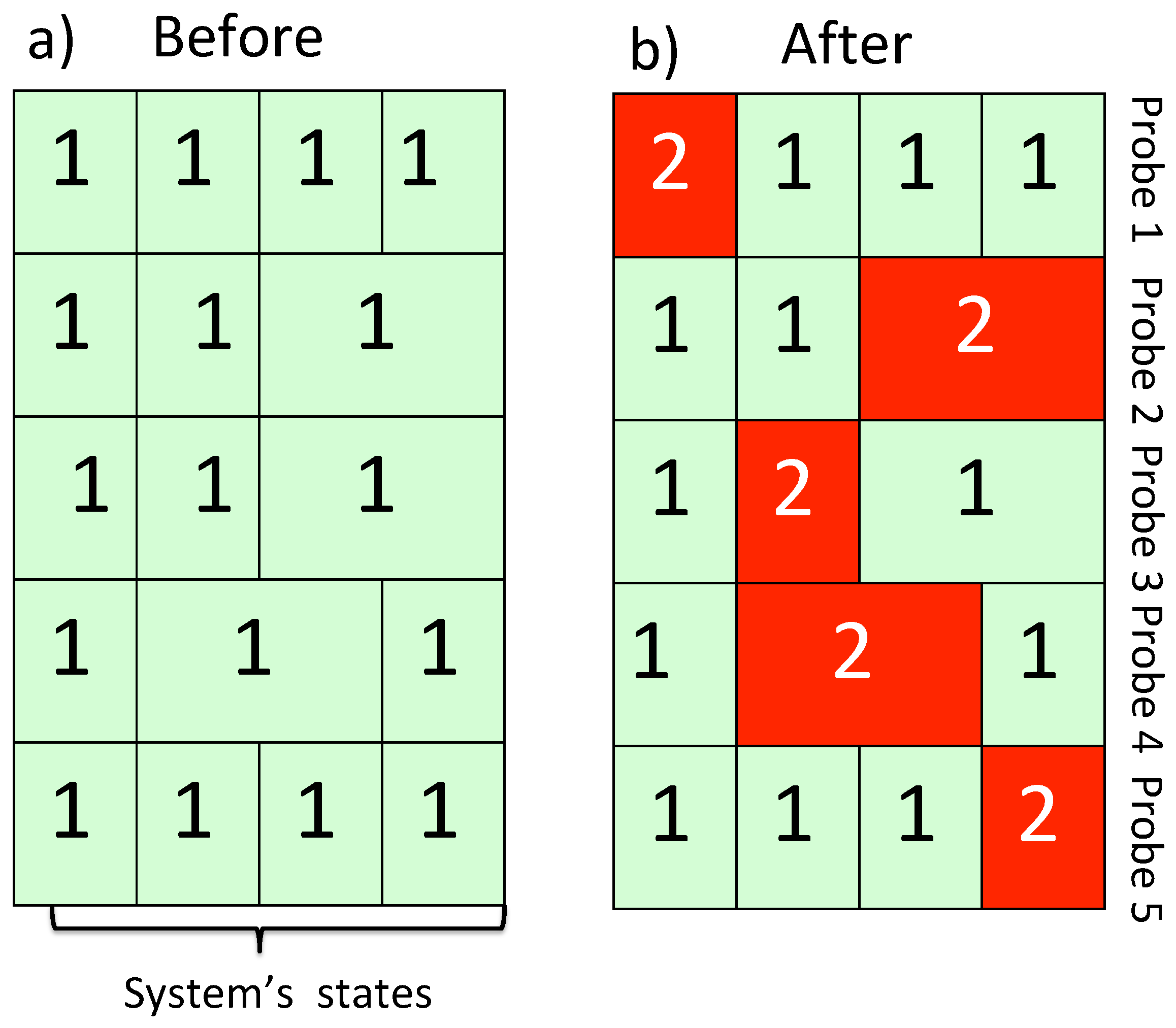
where, as before, we we assumed , , and . The experimenter prepares all probes in the states (14) and, once the experiment is finished, only needs to check which sub-system of , say, the -th, has changed its state. This will tell him/her that the value of at was . As a simple example, Figure 3 shows an outcome of five measurements made on a four-state system. There the first probe, capable of distinguishing between all four states prepares the system in a state . The second probe cannot tell apart the third and the second states, so , , and , and so on. The sequence of the measured valued obtained by inspecting the probes at is . After many trials the sequence will be observed with a probability [cf. Equation (5)]
4.2. Von Neumann’s Pointers
In classical mechanics one can measure the value of a dynamical variable at by coupling the system to a “pointer”, a heavy one-dimensional particle with position f and momentum . The full Hamiltonian is given by , and at the pointer is rapidly displaced by , which providies the desired reading. What happens to the system, depends on the pointer’s momentum, which remains unchanged by the interaction. If , the system continues on its way unperturbed. If , the system experiences a sudden kick, whereby its position and momentum are changed by and , respectively.
The quantum version of the pointer [20] employs a coupling , where , is the pointer’s momentum operator, and is the (system’s) operator to be measured. The function can be chosen constant for the duration of the measurement , , and zero otherwise. It tends to a Dirac delta for an instantaneous (impulsive) measurement, where . For a system whose state lies in the eigen sub-space of a projector , the action of results in a spatial shift of the pointer’s initial state by ,
With pointers employed to measure quantities , the initial state of the composite can be chosen to be [cf. Equation (9)]
where the initial pointer states can be, e.g., identical Gaussians of a width , all centred at the origin,
except for the first probe, where we would need a narrow Gaussian, in order to prepare the system in . If all couplings are instantaneous, for the amplitude in Equation (3) [with , and replaced by a state of the composite, , ] one finds
where, again, is the system’s amplitude (3).
If one wants their measurements to be accurate, the pointers need to be set to zero with as little uncertainty as possible (see. Figure 4). This uncertainty is determined by the Gaussian’s width , and sending it to zero we have [since and for any ]
where is the probability, computed with the help of Equation (7).
Equation (24) is the desired result, which deserves a brief discussion. In each trial, the pointers’ readings may take only discrete values , and the observed sequences occur with the probabilities, predicted for the system by Feynman’s rules of Section 2. However, unlike in the classical case, this information comes at the cost of perturbing the system’s evolution. Indeed, writing and proceeding as before, one obtains terms like , where represents the “kick”, produced on the system by the ℓ-th pointer at . As in the classical case, we can get rid of the kick by ensuring that the pointer’s momentum is approximately zero. However, Heisenberg’s uncertainty principle (see, e.g., [1]) will make the uncertainty in the initial pointer position very large. Accuracy and perturbation go hand in hand, and the measured values do not “pre-exist” measurements but are produced in the course of it [21]. Notably, one can still predict the probabilities by not mentioning the pointers at all and analyzing instead an isolated system, whose unitary evolution is broken each time the coupling takes place.
Secondly, and importantly, von Neumann pointers have many states, and only a few of them are actually used. This suggests that the pointers and the probes of the previous section could, in principle, be replaced by much more complex devices, with only a few states of their vast Hilbert spaces coming into play. For example, there is nothing in quantum theory that forbids using printers, which print the observed values on a piece of paper. If an experiment that measures spin’s component is set properly, the machine will print only “up” or “down” with the predicted frequencies, and would never digress into French romantic poetry.
5. The Past of a Quantum System: Elements of Reality
The stock of an experiment described so far, is taken just after the last measurement at . This is the “present” moment, the times are relegated to the “past”, and the “future” is yet unknown. Possible pasts are defined by the choice of the measured quantities , and of the times at which the impulsive measurements are performed. The possible outcomes occur with probabilities which the theory aims to predict. There are clearly gaps in the description of the system between successive measurements at and . One way to fill them (without adding new measurements, which would change the problem) is to look for quantities whose values can be ascertained at some without altering the existing probabilities . Or, to put it slightly differently, to ask what can be measured without destroying the interference between the virtual paths [cf. (2)] which contribute to the amplitudes in Equation (3).
There is a well-known analogy. EPR-like scenarios [22] are often used to question the manner in which quantum theory describes the physical world. In a nutshell, the argument goes as follows. Alice and Bob, at two separate locations, share an entangled pair of spins. Alice can ascertain that Bob’s spin has any desired direction, while apparently unable to influence it due to the restrictions imposed by special relativity. Hence, all possible values of the spin’s projections can exist simultaneously, i.e., be in some sense real. If quantum mechanics insists that different projections cannot have well-defined values at the same time, it must be incomplete. We are not interested here in the details of this important ongoing discussion (for an overview see [22] and Refs. therein), or the implications relativity theory may have for elementary quantum mechanics [23]. Rather we want to make use of the Criterion of Reality (CR) used by the authors of [24] to determine what should be considered “real”. This criterion reads: “If, without in any way disturbing a system, we can predict with certainty (i.e., with probability equal to unity) the value of a physical quantity, then there exists an element of reality corresponding to that quantity.” [24].
Consider again an experiment in which measurements are made on the system at , , while the system’s condition at some between, say, and remains unknown. To fill this gap, one may use the CR criterion just cited, and look for any information about the system, which can be obtained without altering the existing statistical ensemble. Thus, one needs a variable whose measurement at results is
There are at least two kinds of quantities that satisfy this condition. To the first kind belong operators of the type
where is the projector evolved backwards in time from to . To the second kind belong the quantities
where is the projector evolved forwards in time from to . Indeed, since and , we have
and [cf. Equation (6)]
There is, of course, a simple explanation. The states form an orthogonal basis for measuring , and the system in at can only go to at , as all other matrix elements of vanish. Similarly, the system in at can only go to at . The presence of the operators and in Equations (26) and (27) ensures that Equation (25) holds, and Equation (29) follow.
The problem is as follows. By using the CR, we appear to be able to say that at a quantity has a definite value if the value of at was . Similarly, it would appear that also has a definite value if the value of at is Since in general and do not commute, , and quantum mechanics forbids ascribing simultaneous values to non-commuting quantities, we seem to have a contradiction.
Fortunately, the contradiction is easily resolved. At the end of the experiment, one needs to have all the relevant records and to produce these records an additional probe must be coupled at . Measuring , or requires different probes, which affect the system differently, and produce different statistical ensembles. The values and do not pre-exist in their respective measurements [9,21], and appear as a result of a probe acting on a system. The caveat is the same as in Bohr’s answer [25] to the authors of [24]. There are no practical means of ascertaining these conflicting values simultaneously. Next, we give a simple example.
6. A Two-Level Example
Consider a two-level system, (a qubit), , prepared by the first measurement of an operator
in a state at . The second measurement (we have ) yields one of the eigenvalues of an operator
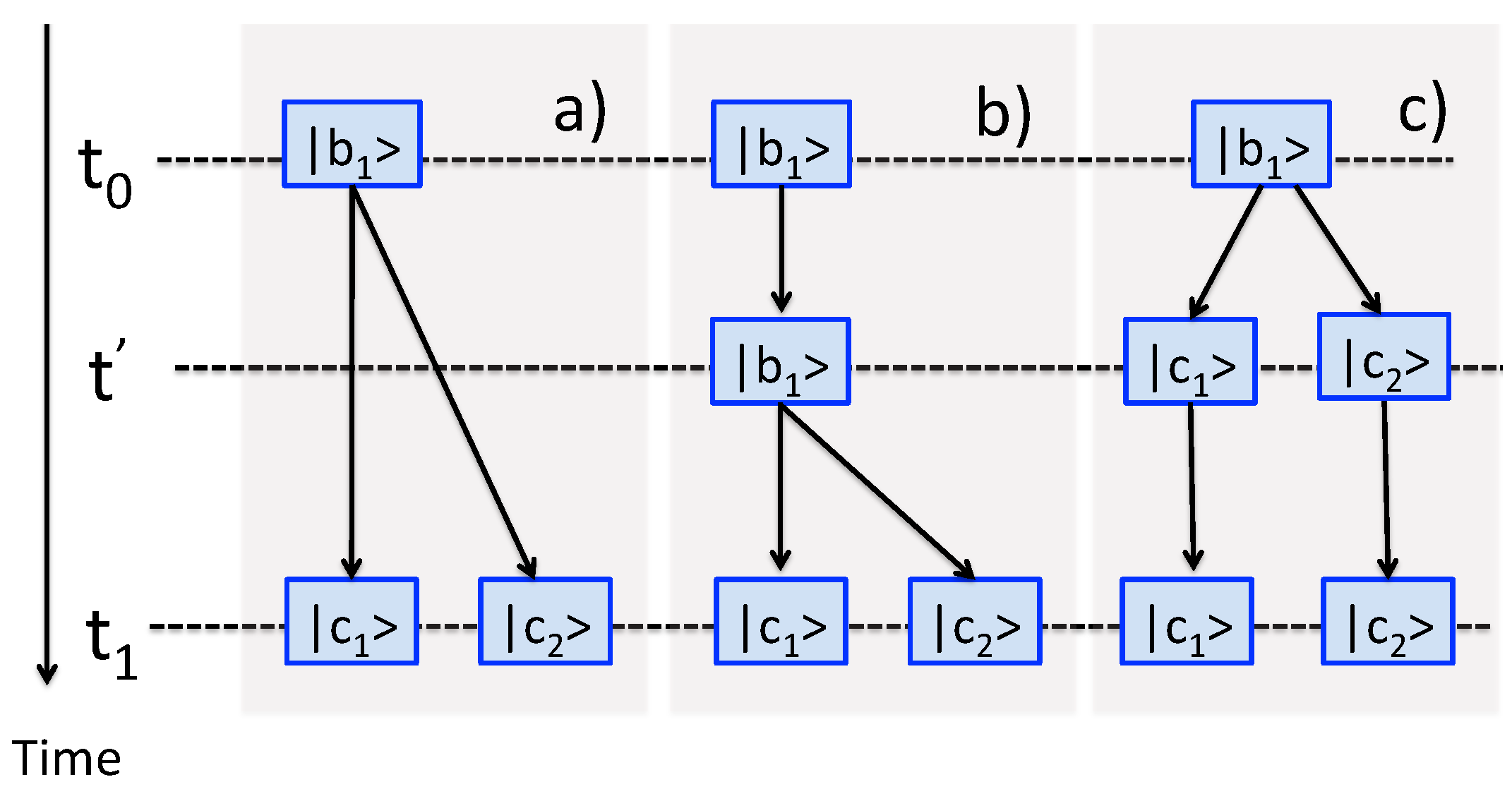
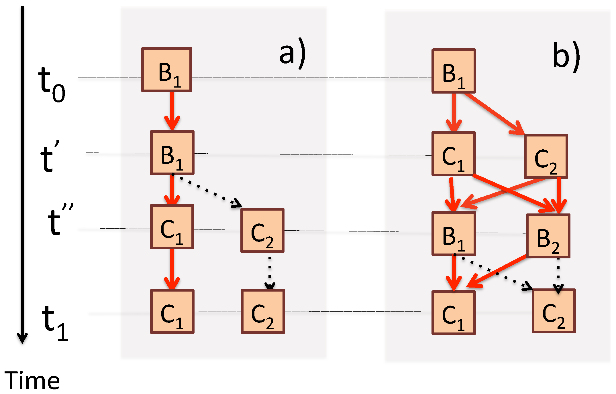
With only two dimensions involved, all eigenvalues are non-degenerate. If for simplicity we put , (see Figure 5a), one can easily verify that at any the value of is (see Figure 5b), or that has the same value it will have at (see Figure 5c). Moreover, its is easy to ascertain that if the first and the last outcomes are and , the values of at and of at are and , as long as (see Figure 6a). Indeed, according to (3) we have
The former is no longer true if is measured before . A final value can now be reached via four real paths shown in Figure 6b, and the probabilities no longer agree with those Equation (32),
The transition between the two regimes occurs at , when an attempt is made to measure two non-commuting quantities at the same time. The rules of Section 2 imply that such measurements are not possible in principle, since and do not have a joint set of eigenstates which could inserted into Equation (2). However, ultimately one is interested in the records available at the end of the experiment. Next, we will look at the readings the probes would produce, should they be set up to measure non-commuting and simultaneously.
7. Joint Measurement of Non-Commuting Variables
We want to consider two measurements made on the system in Figure 6 which can overlap in time at least partially. No longer instantaneous, both measurement will last seconds, start at and , , respectively, and finish before , . The degree to which the measurements overlap will be controlled by a parameter ,
so that for the measurement of precedes that of , corresponds to simultaneous measurements of both and , and for is measured first. Next we consider the two kind of probes introduced in Section 4 separately.
7.1. C-NOT Gates as a Meters
For our two-level example of Section 6 we can further simplify the probe described in Section 4. Since we only need to distinguish between two of the system’s conditions, a two-level probe, whose state either changes or remains the same, is all that is required. We will need two such probes, and , two sets of states
four projectors
and two couplings
where . In what follows we will put . The probes are prepared in the respective states and , and after finding the system in at their state is given by
if , while for the order of operators in (38) is reversed. It is easy to check that ()
so that for the r.h.s. of Equation (39) reduces to . The action of the coupling is, therefore, that of a quantum (C)ontrolled-NOT gate [26], which flips the probe’s (target) state if the system’s (control) state is or , and leaves the probes’s condition unchanged if it is or .
There are four possible outcomes, , , , and , and four corresponding probabilities (i, j = 1, 2),
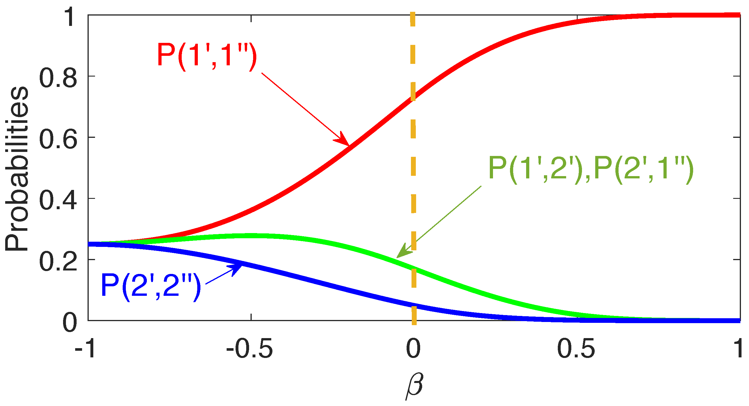
The matrix elements are easily evaluated (for details see Appendix B), and the results are shown in Figure 7.
If , there is no overlap, and is measured before . Dividing into K sub-intervals and sending we have an identity (cf. Equation (39))
and the state of the first probe remains unchanged. For both probes act simultaneously. Now the use of the Trotter’s formula yields
Equation (42) contains scenarios where both probes change their states, and since , the evolution of one of them must affect what happens to the other. Now all four probabilities in Equation (40) have non-zero values, although it is still more likely that both probes will remain in their initial states (cf. Figure 7). Finally, for , is measured before as if both measurements were instantaneous, and all four paths in Figure 6b are equally probable. A different result is obtained if the two measurements are of von Neumann type, as we will discuss next.
7.2. Von Neumann Meters
Consider the same problem but with the two-level probes replaced by two von Neumann pointers with positions and , respectively. As before, the interaction with each pointer lasts seconds, so the two Hamiltonians are
If the pointers are prepared in identical Gaussian states (22) the probability distribution of their final positions is given by
where (we measure f in units of and put )
where , , and . (For we interchange with .)
Consider first the case where the measurements coincide. The amplitude has several general properties. Firstly, it cannot be a smooth finite function of and , or the integral in (44) would vanish in the limit of narrow Gaussians, , due to the normalisation of and (cf. Equation (22)). It must, therefore, have -singularities [27,28]. Secondly, using the Trotter’s formula [29], we have
It is readily seen that each time the product in the r.h.s. of Equation (46) is applied, the pointers are displaced by or and or , respectively. If , one has a quantum random walk, where the pointers are shifted by an equal amount ether to the right or to the left. Since the largest possible displacement is 1, must vanish outside a square . One also notes that for , the maximum of is reached for , since there are (let K be an even number) walks, each contributing to the same amount . Similarly, a maximum of is reached for .
A detailed combinatorial analysis is complicated, but the location of the singularities can be determined as was done in [30]. As explained in the Appendix B, the amplitude in Equation (45) can also be written as (, )
where is the Bessel function of the first kind of order k. From Equation (44) one notes that in the limit , in Equation (44) will become singular, and that its singularities will coincide with those of in Equation (45). Since [31]
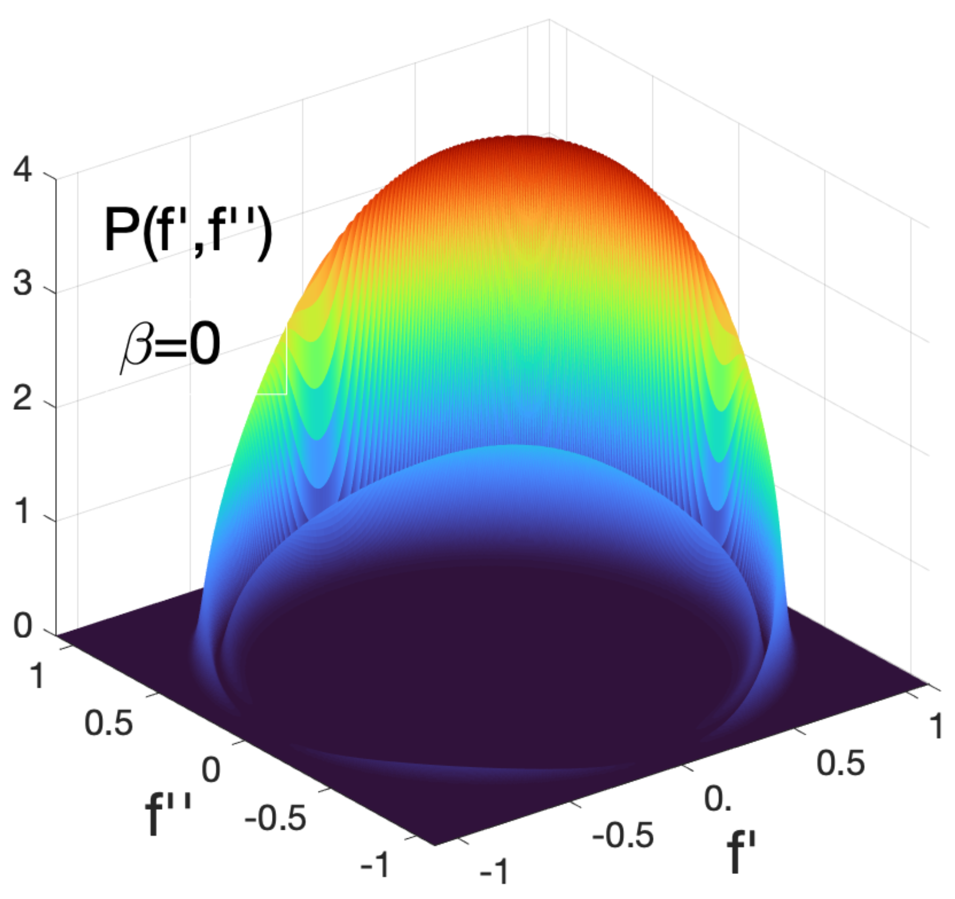
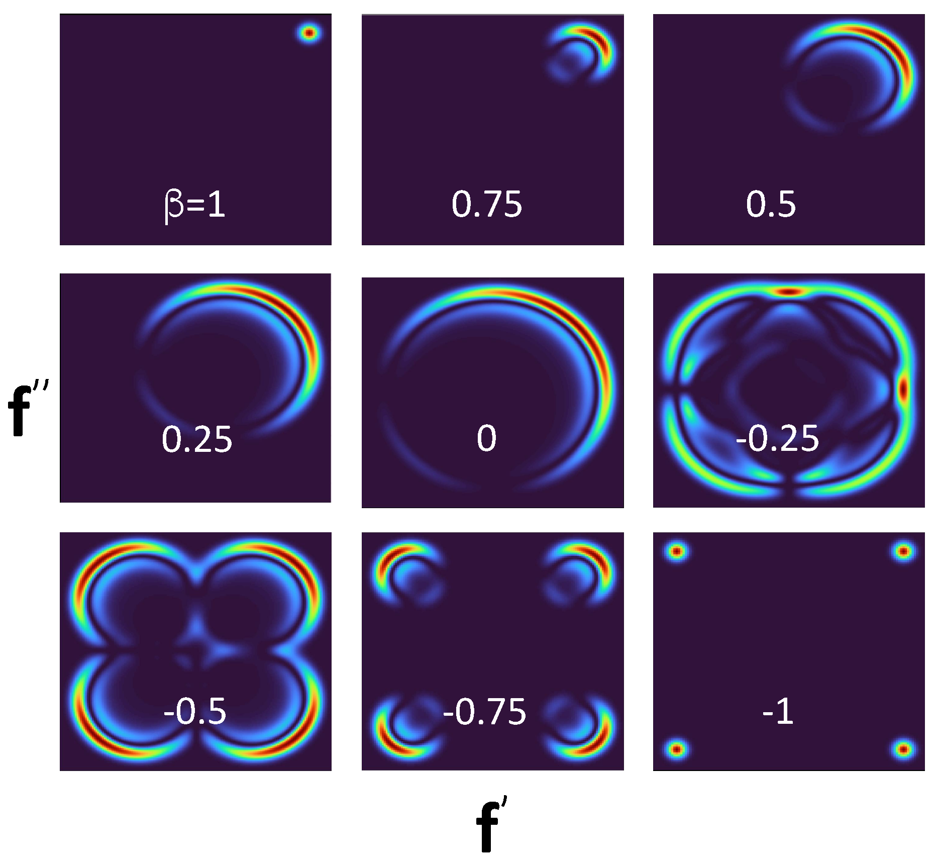
the integral in Equation (47) will diverge at large ’s provided the oscillations of and are cancelled by those of and , i.e., for . As a result, we find the pointer readings of two simultaneous accurate measurements of and (with ) distributed along the perimeter of a unit circle as shown in Figure 8. Figure 9 shows the distribution of the pointer’s readings for different degrees of overlap between the two measurements.
There is, therefore, an important difference between employing discrete probes and von Neumann pointers. In the previous example shown in Figure 7 one could (although should not) assume, e.g., that for yields the probability for and to have the values 1 and , if measured simultaneously. Figure 8 and Figure 9 show this conclusion to be inconsistent. As decreases from 1 to , the pointer’s readings are not restricted to , . Rather, for they are along the perimeters of a unit circle (cf. Figure 8 and Figure 9), which, if taken at face value, implies that the probability in question is zero. We already noted that the theory in Section 2 is unable to prescribe probabilities of simultaneous values of non-commuting operators. In practice, this means that the probes, capable of performing the task in a consistent manner, simply cannot be constructed.
8. The Past of a Quantum System: Weakly Perturbing Probes and the Uncertainty Principle
It remains to see what information can be obtained from the measurements, designed to perturb the measured system as little as possible. If such a measurement were an attempt to distinguish between interfering scenarios, without destroying interference between them, it would contradict the Uncertainty Principle cited in Section 2. As before, we treat the two types of probes separately.
8.1. Weak Discrete Gates
We start by reducing the coupling strength, so the interaction Hamiltonians (15) become
In [11], Feynman described a double-slit experiment where photons, scattered by the the passing electron, allowed one to know through which of the two slits the electron has travelled. With every electron duly detected, their distribution on the screen, , does not exhibit an interference pattern. With no photons present, the pattern is present in the distribution . If the intensity of light (i.e., the number of photons) is decreased, some of the electrons pass undetected. The total distribution on the screen is, therefore, “a mixture of the two curves” [11]. , where a and b are some constants.
Something very similar happens if an extra discrete probe is added to measure at , . As before [cf Equation (16)], we find
where the cosine term accounts for the possibility that the systems passes the check undetected. Replacing in Feynman’s example with the probability of detecting the system in a final state at . With a values of detected in every run, , one has a distribution
where is the amplitude in Equation (5). If the probe is uncoupled, , the distribution is
With the outcomes fall into two groups, those where the probe remains in its initial state, and those where the state of one of its sub-systems has been flipped. The two alternatives are exclusive [32], and the total distribution is indeed a mixture of the two curves. As one has
In other words, in the vast majority of cases, the system remains undetected, and the interference is preserved (cf. Equation (52)). In the few remaining cases, it is detected and the interference is destroyed. The Uncertainty Principle [1] is obeyed to the letter: probabilities are added where records allow one to distinguish between the scenarios; otherwise one sums the amplitudes. One has, however, to admit that nothing really new has been learned from this example, as both possibilities simply illustrate the rules of Section 2.
The above analysis is easily extended to include more extra measurements, whether impulsive or not. Since to the first order in the coupling constant weak probes act independently of each other, the r.h.s. of Equation (53) would contain additional terms , , etc.
8.2. Weak von Neumann Pointers
Next we add to accurate impulsive von Neumann pointers an extra “weak” pointer, designed to measure at between and . The new coupling, given by
will perturb the system only slightly in the limit . To see what happens in this limit, one can replace by , in Equation (54) by , and the pointer’s initial state by . Now as the pointer’s initial states become very broad, while the coupling remains unchanged. For a Gaussian pointers (22), considered here, this means replacing with , i.e., making the measurement highly inaccurate. This makes sense. The purpose of a pointer is to destroy interference between the system’s virtual paths, (cf. Equation (24)), which it is clearly unable to do if the coupling vanishes. Accordingly, with the pointer’s initial position highly uncertain, its final reading is also spread almost evenly between and ∞. Measured in this manner, the value of remains indeterminate, as required by the Uncertainty Principle.
This could be the end of our discussion, except for one thing. It is still possible to use the broad distribution of a pointer’s readings in order to evaluate averages, which could, in principle, remain finite in the limit . Maybe this can tell us something new about the system’s condition at . Note, however, that whatever information is extracted in this manner should not contradict the Uncertainty Principle, or the whole quantum theory would be in trouble [1].
From Equation (22) it is already clear that any average of this type will be expressed in terms of the amplitudes . The simplest average is the pointer’s mean position. If the outcomes of the accurate measurements are , for the mean reading of the weakly coupled pointer we obtain (see Appendix C)
If the measured operator is one of the projectors, say, , this reduces to
We note that, as in the previous example, different pointers do not affect each other to the leading order in the small parameter .
The quantities in the l.h.s. of Equations (55) and (56) are the standard averages of the probes’ variables. In the l.h.s. of these equations one finds probability amplitudes for the system’s entire paths, . The values of these amplitudes can be deduced from the probes’s probabilities [33]. The problem is, these values offer no insight into the condition of the system at . In the double-slit case, to conclude that a particle “...goes through one hole or the other when you are not looking is to produce an error in prediction” [11]. In our case, one cannot say that the value of was or was not a particular . The Uncertainty Principle prevails again, this time by letting one only gain information not sufficient for determining the condition of the unobserved system at . A more detailed discussion of this point can be found, e.g., in [7,8].
9. Summary and Conclusions
A very general way to describe quantum mechanics is to say that it is a theory that prescribes probability amplitudes to sequences of events, and then predicts the probability of a sequence by taking an absolute square of the corresponding amplitude [1]. Where several () consecutive measurements are made on the same system (S), a sequence of interest is that of the measured values , endowed with a (system’s) probability amplitude in Equation (5).
This is not, however, the whole story. To test the theory’s predictions, an experimenter (Observer) must keep the records of the measured values, in order to collect the statistics once the experiment is finished. This is more than a mere formality. The system, whose condition changes after each measurement, cannot itself store this information. Hence the need for the probes, material objects, whose conditions must be directly accessible to the Observer at the end. One can think of photons [1,11] devices with or without dials, or Observer’s own memories of the past outcomes [17,18]. The probes must be prepared in suitable initial condition and be found in one of the orthogonal states later, with an amplitude , .
To be consistent, the theory must construct the amplitudes and using exactly the same rules, and ensure that . In other words, the experimenter should see a record occurring with a frequency the theory predicts for an isolated (no probes) system, going through its corresponding conditions. This requires the existence of a suitable coupling between the system and the probe. Its choice is not unique, and for a system with a finite-dimensional Hilbert space studied here, two different kinds of probes were discussed in Section 4. The first one is a discrete gate, using the interaction in Equation (15), while the second is the original von Neumann pointer [20].
Now one can obtain the same probability by considering a unitary evolution of a composite until the moment the Observer examines their records at the end of the experiment. Or one can consider such an evolution of the system only, but broken every time a probe is coupled to it. For a purist intent on identifying quantum mechanics with unitary evolution (see, e.g., the discussion in [34]), the first way may seem preferable. Yet there is no escaping the final collapse of the composite’s wave function when the stock is taken at the end of the experiment.
It is often simpler to discuss measurements in terms of the measured system’s amplitude, leaving out, but not forgetting, the probes. The rules formulated in Section 2 readily give an answer to any properly asked question, but offer no clues regarding a question which has not been asked operationally. One may try to extend the description of a quantum system’s past by looking for additional quantities whose values could be ascertained without changing the probabilities of the measured outcomes. In general, this is not possible. To find the value of a quantity at a between to successive measurements, , one needs to connect an extra probe. This would destroy interference between the system’s paths and change other probabilities, leaving the question “what was the value of if was not measured?” without an answer.
There are two seeming exceptions to this rule. If is obtained by evolving backward in time the previously measured (cf. Equation (26)), call it , its value is certain to equal that of , and all other probabilities will remain unchanged, (cf. Equation (28)). Similarly, the value of a (cf. Equation (27)), obtained by the forward evolution of the next measured operator , will also agree with that of . It would be tempting to assume that these values represent some observation-free “reality”, were it not for the fact that they cannot be ascertained simultaneously. The two measurements require different probes, each affecting the system in a particular way. The probes frustrate each other if employed simultaneously. It is hardly surprising that different evolution operators , in Equation (10) may lead to different outcomes.
One notes also that measuring these two quantities one after another would also leave all other probabilities intact, but only if is measured first, as shown in Figure 6a. Changing this order results in a completely different statistical ensemble, shown in Figure 6b. The rules of Section 2 say little about what happens if the measurements coincide, except that if and do not have common eigenstates, Equation (5) cannot be applied. One can still analyze the behavior of the two probes at different degrees of overlap to explain why it is impossible to reach consistent conclusions about the simultaneous values of and . For example, if two discrete gates are used, Figure 7 appears to offer four joint probabilities of having the values . If discrete probes are replaced by von Neumann pointers, the readings shown in Figure 8 suggest that joint values of and should lie on the perimeter of a unit circle, in a clear contradiction with the previous conclusion.
Another way to explore the system’s past beyond what has been established by accurate measurements, is to study its response to a weakly perturbing probe, set up to measure some at an intermediate time . In this limit, the two types of probes produce different effects but, in accordance with the Uncertainty Principle, reveal nothing new that can be added to the rules formulated in Section 2. If the coupling of an additional discrete probe is reduced, trials are divided into two groups. In a (larger) number of cases, the system remains undetected, and interference between its virtual paths passing through different eigenstates of remains intact. In a (smaller) fraction of cases, the value of is accurately determined, and the said interference is destroyed completely. Individual readings of a weak von Neumann pointer extend a range much wider than the region which contains the values of , and are in this sense practically random. Its mean position (reading) allows one to learn something about the probability amplitude in Equation (56), or a combination of such amplitudes as in Equation (55). The problem is that even after obtaining the values of these amplitudes (and this can be done in practice [33]), one still does not know the value of , for the same reason he/she cannot know the slit chosen by an unobserved particle in a double-slit experiment. Quantum probability amplitudes simply do not have this kind of predictive power [1,11].
In summary, quantum mechanics can consistently be seen as a formalism for calculating transition amplitudes by means of evaluating matrix elements of evolution operators. In such a “minimalist” approach (see also [35]), the importance of a wave function, represented by an evolving system’s state, is reduced to that of a convenient computational tool. In the words of Peres [23] (see also [36]) “... there is no meaning to a quantum state before the preparation of the physical system nor after its final observation (just as there is no ‘time’ before the big bang or after the big crunch).” This is, however, not a universally accepted view. For example, the authors of [4,5,6] propose a time-symmetric formulation of quantum mechanics, employing not one but two evolving quantum states. We will examine the usefulness of such an approach in future work.
Funding
This research was funded by the Basque Government, Grant No. IT986-16, and of MINECO, the Ministry of Science and Innovation of Spain, Grant PGC2018-101355-B-100(MCIU/AEI/FEDER,UE).
Institutional Review Board Statement
Not applicable.
Informed Consent Statement
Not applicable.
Data Availability Statement
Not applicable.
Conflicts of Interest
The author declares no conflict of interest.
Appendix A
Evaluation of the Probabilities in Equation (40). For the eigenstates of the probes’s operators we have
Appendix B
Derivation of Equation (47). The two-level system (a spin-), with , is pre- and post-selected in the states and , , . respectively. Two pointers are employed to measure and simultaneously, . (Extension to measurements along non-orthogonal axes is trivial.) The final distribution of the pointer’s positions (readings) is, therefore, given by
where and
We recall that
where , and . Defining , , we obtain , where .
Appendix C
Derivation of Equation (55). Consider impulsive von Neumann pointers accurately measuring the quantities . and have non-degenerate eigenvalues, the first measurement yields an outcome and leaves the system in a state . The last measurement yields and leaves the system in . An extra weakly coupled pinter is added at , to measure . Just after the state of the pointers is given by
where , , and is very broad, so that . For the distribution of the readings we have
and the (unnormalised) distribution of the weak pointer’s readings given that the other outcomes are is given by ()
where we expanded the (broad) to the first order in its (small) derivatives. For a Gaussian pointer is given by Equation (22), , and . Defining
and integrating by parts, yields Equation (55).
References
- Feynman, R.P.; Leighton, R.; Sands, M. The Feynman Lectures on Physics III; Dover Publications, Inc.: New York, NY, USA, 1989; Ch.1: Quantum Behavior. [Google Scholar]
- Frauchiger, D.; Renner, R. Quantum theory cannot consistently describe the use of itself. Nat. Commun. 2018, 9, 3711. [Google Scholar] [CrossRef] [PubMed]
- Sokolovski, D.; Matzkin, A. Wigner’s Friend Scenarios and the Internal Consistency of Standard Quantum Mechanics. Entropy 2021, 23, 1186. [Google Scholar] [CrossRef] [PubMed]
- Aharonov, Y.; Vaidman, L. Complete description of a quantum system at a given time. Phys. A Math. Gen. 1991, 24, 2315. [Google Scholar] [CrossRef]
- Aharonov, Y.; Popescu, S.; Tollaksen, J. A Time-symmetric Formulation of Quantum Mechanics. Phys. Today 2010, 63, 11. [Google Scholar] [CrossRef] [Green Version]
- Robertson, K. Can the two-time interpretation of quantum mechanics solve the measurement problem? Stud. Hist. Philos. Mod. Phys. 2017, 58, 54–62. [Google Scholar] [CrossRef] [Green Version]
- Sokolovski, D. Weak measurements measure probability amplitudes (and very little else). Phys. Lett. A 2016, 380, 1593–1599. [Google Scholar] [CrossRef] [Green Version]
- Sokolovski, D.; Akhmatskaya, E. An even simpler understanding of quantum weak values. Ann. Phys. 2018, 388, 382–389. [Google Scholar] [CrossRef]
- Sokolovski, D. Path probabilities for consecutive measurements, and certain “quantum paradoxes”. Ann. Phys. 2018, 397, 474–502. [Google Scholar] [CrossRef] [Green Version]
- Bohr, N. Space and Time in Nuclear Physics. Manuscript Collection, Archive of the History of Quantum Physics. Master’s Thesis, American Philosophical Society, Philadelphia, PA, USA, 21 March 1935. [Google Scholar]
- Feynman, R.P. The Character of Physical Law; M.I.T. Press: Cambridge, MA, USA; London, UK, 1985. [Google Scholar]
- Peres, A. Consecutive quantum measurements. In Quantum Theory without Reduction; Cini, M., Levy-Leblond, J.-M., Eds.; IOP Publishing: Bristol, UK, 1990. [Google Scholar]
- Gudder, S.; Nagy, G. Sequential quantum measurements. J. Math. Phys. 2001, 42, 5212–5222. [Google Scholar] [CrossRef]
- Nagali, E.; Felicetti, S.; de Assis, P.-L.; D’Ambrosio, V.; Filip, R.; Sciarrino, F. Testing sequential quantum measurements: How can maximal knowledge be extracted? Sci. Rep. 2012, 2, 443. [Google Scholar] [CrossRef] [Green Version]
- Fields, D.; Bergou, A.; Varga, A. Sequential measurements on qubits by multiple observers: Joint Best Guess strategy. In Proceedings of the 2020 IEEE International Conference on Quantum Computing and Engineering (QCE), Denver, CO, USA, 12–16 October 2020; p. 235. [Google Scholar] [CrossRef]
- Glick, J.R.; Adami, C. Markovian and Non-Markovian Quantum Measurements. Found. Phys. 2020, 50, 1008–1055. [Google Scholar] [CrossRef]
- Matzkin, A.; Sokolovski, D. Wigner’s friend, Feynman’s paths and material records. EPL 2020, 131, 40001. [Google Scholar] [CrossRef]
- Sokolovski, D. Quantum Measurements with, and Yet without an Observer. Entropy 2020, 22, 1185. [Google Scholar] [CrossRef] [PubMed]
- Sudbery, A. Histories Without Collapse. Int. J. Theor. Phys. 2022, 61, 39. [Google Scholar] [CrossRef]
- von Neumann, J. Mathematical Foundations of Quantum Mechanics; Princeton University Press: Princeton, NJ, USA, 1955; Chapter VI. [Google Scholar]
- Mermin, N.D. Hidden variables and the two theorems of John Bell. Rev. Mod. Phys. 1993, 65, 803. [Google Scholar] [CrossRef]
- Fine, A. The Einstein–Podolsky–Rosen Argument in Quantum Theory; The Stanford Encyclopedia of Philosophy (Summer 2020 Edition); Zalta, E.N., Ed.; Available online: https://plato.stanford.edu/archives/sum2020/entries/qt-epr/ (accessed on 8 June 2022).
- Peres, A. Relativistic quantum measurements in Fundamental Problems of Quantum Theory. Ann. N. Y. Acad. Sci. 1995, 455. [Google Scholar] [CrossRef]
- Einstein, A.; Podolsky, B.; Rosen, N. Can quantum-mechanical description of physical reality be considered complete? Phys. Rev. 1935, 47, 777–780. [Google Scholar] [CrossRef] [Green Version]
- Bohr, N. Can quantum-mechanical description of physical reality be considered complete? Phys. Rev. 1935, 48, 696–702. [Google Scholar] [CrossRef]
- Barenco, A.; Bennett, C.H.; Cleve, R.; DiVincenzo, D.P.; Margolus, N.; Shor, P.; Sleator, T.; Smolin, J.A.; Weinfurter, H. Elementary gates for quantum computation. Phys. Rev. A 1995, 52, 3457–3467. [Google Scholar] [CrossRef] [Green Version]
- Sokolovski, D. Zeno effect and ergodicity in finite-time quantum measurements. Phys. Rev. A 2011, 84, 062117. [Google Scholar] [CrossRef] [Green Version]
- Sokolovski, D. Path integral approach to space-time probabilities: A theory without pitfalls but with strict rules. Phys. Rev. D 2013, 87, 076001. [Google Scholar] [CrossRef] [Green Version]
- Trotter, H.F. On the product of semi-groups of operators. Proc. Am. Math. Soc. 1959, 10, 545–551. [Google Scholar] [CrossRef]
- Sherman, E.Y.; Sokolovski, D. Von Neumann spin measurements with Rashba fields. New J. Phys. 2014, 16, 015013. [Google Scholar] [CrossRef]
- Abramowitz, M.; Stegun, I.A. Handbook of Mathematical Functions; Applied Mathematics Series; U.S. GPO: Washington, DC, USA, 1964.
- Feynman, R.P.; Hibbs, A.R. Quantum Mechanics and Path Integrals; McGrawHill: New York, NY, USA, 1965. [Google Scholar]
- Martínez-Garaot, S.; Pons, M.; Sokolovski, D. From Quantum Probabilities to Quantum Amplitudes. Entropy 2020, 22, 1389. [Google Scholar] [CrossRef] [PubMed]
- Kastner, R.E. Unitary-Only Quantum Theory Cannot Consistently Describe the Use of Itself: On the Frauchiger-Renner Paradox. Found. Phys. 2020, 50, 441–456. [Google Scholar] [CrossRef] [Green Version]
- Sokolovski, D. A minimalist’s view of quantum mechanics. EPL 2019, 128, 50001. [Google Scholar] [CrossRef]
- Fuchs, C.A.; Peres, A. Quantum Theory Needs No “Interpretation”. Phys. Today 2000, 53, 70. [Google Scholar] [CrossRef] [Green Version]
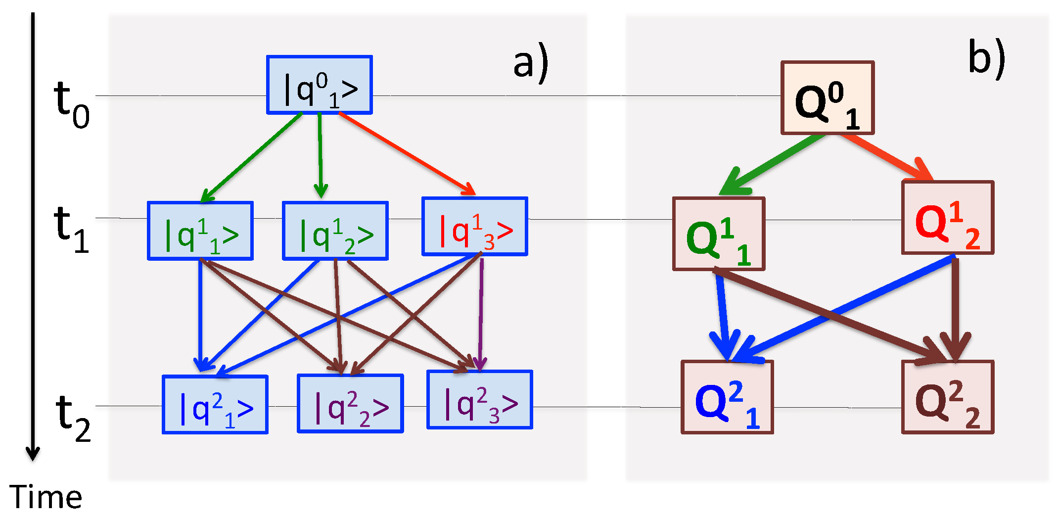
Figure 1.
Three measurements, , are made on a three-level system, . The first one, yields an outcome and prepares the system in a state . Two other operators have degenerate eigenvalues, , (), and , (). (a) Nine virtual paths in Equation (3). (b) Four real paths (i.e., the observed sequences ), . Different colours are used to relate the virtual paths to the observed outcomes.

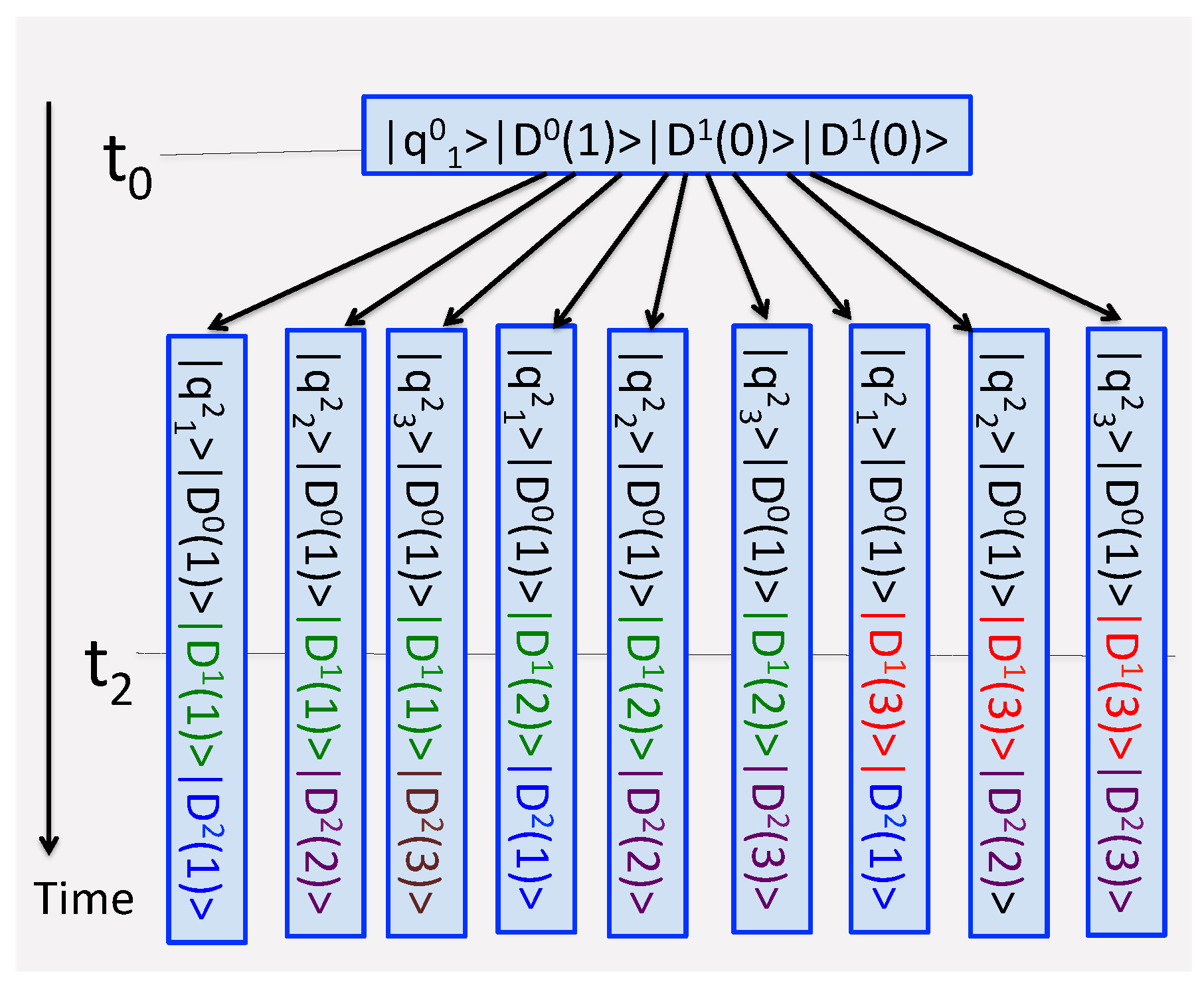
Figure 2.
The measurements in Figure 1 seen from a different perspective. Just after , the experimenter needs to compare three records, in order to determine which of the real paths in Figure 1b was actually taken. This information is encoded in the final conditions of the three probes, , . The composite undergoes an unbroken unitary evolution for . There are nine virtual paths ending in distinguishable states of the composite. The same colors are used to indicate which of the nine path probabilities should be added to obtain likelihoods of the four real scenarios in Figure 1b.

Figure 3.
Five consecutive measurements of the quantities are made on a four-level system (. Some of the eigenvalues are degenerate. Each probe consists of [cf. Equation (15)] two-level sub-systems. (a) Initially sub-systems of all probes are prepared in their lower states . (b) At the end of a trial some these states are found changed, and a record is produced.

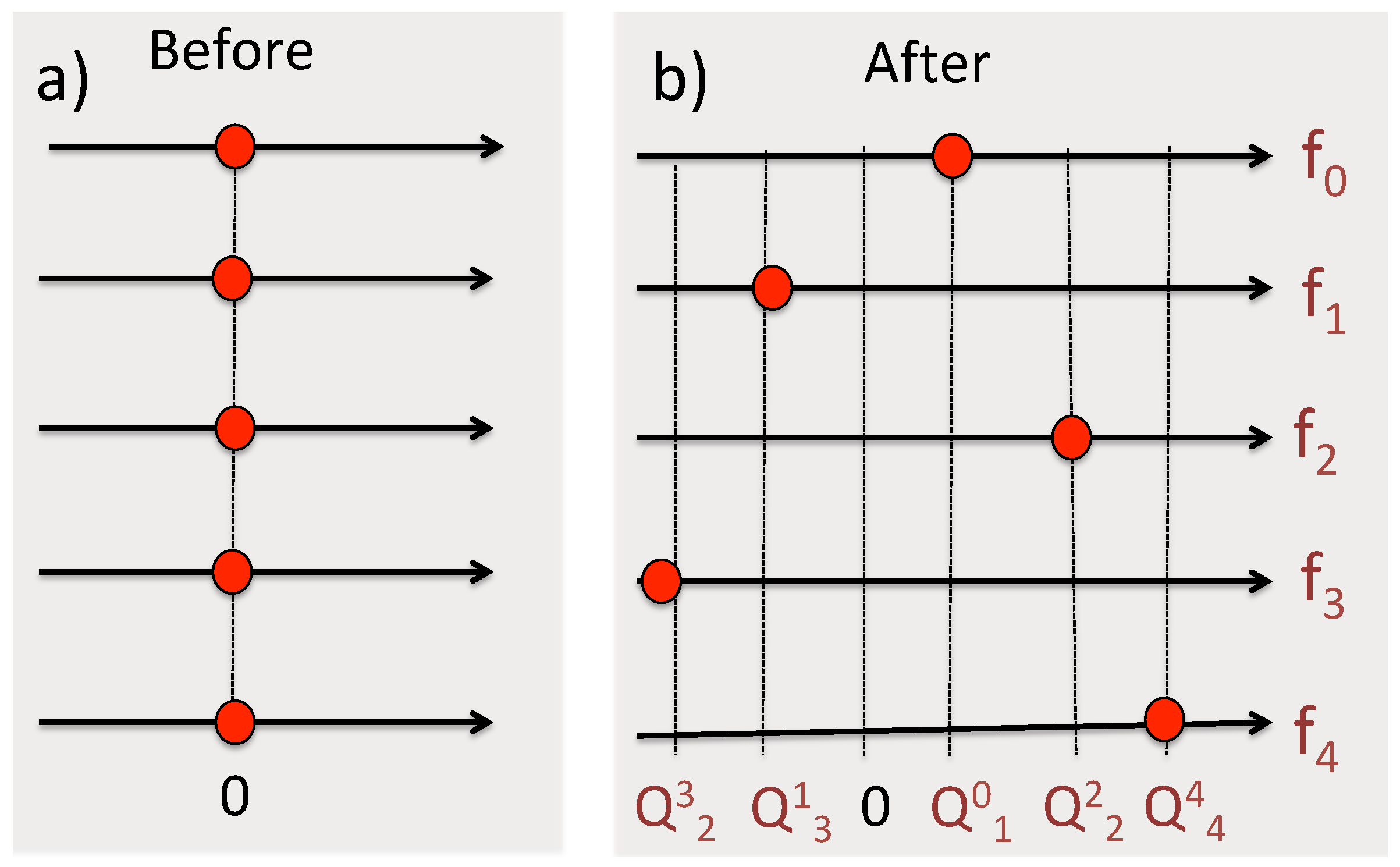
Figure 4.
The measurements shown in Figure 3, this time made by employing five accurate von Neumann pointers. (a) Initially, the pointers are set to zero. (b) At the end of the trial, one finds each pointer shifted by the corresponding eigenvalue. As in Figure 3, an outcome is recorded.

Figure 5.
(a) A measurement of an operator prepares the system () in a state , and is followed by a measurement of . (b) An additional measurement of at yields an outcome , and finds the system in the state with certainty. (c) An additional measurement of at the same yields with certainty, if the last outcome is also . The probabilities are unchanged, , and it would appear that at the system has well defined values of non-commuting operators and .

Figure 6.
(a) In the case shown in Figure 5b, at one can add a measurement of , still leaving the probabilities unchanged, . It would appear that in a transition intermediate values and co-exist for any and , such that . (b) The above is no longer true if is measured before . The transition between the cases (a,b) is discussed in Section 7.

Figure 7.
The values of and are measured jointly (cf. Equations (36)–(38)) for a two-level system (), initially polarised along the x-axis, , , and later found polarised along the y-axis, , . Four probabilities in Equation (40) are plotted vs. in Equation (35). For the measurement of precedes that of , for , and are measured simultaneously, and for , is measured first.

Figure 8.
The values of and are measured simultaneously (, ) for a two-level system (), initially polarised along the x-axis, , , and later found polarised along the y-axis, , .
Figure 8.
The values of and are measured simultaneously (, ) for a two-level system (), initially polarised along the x-axis, , , and later found polarised along the y-axis, , .


Publisher’s Note: MDPI stays neutral with regard to jurisdictional claims in published maps and institutional affiliations. |
© 2022 by the author. Licensee MDPI, Basel, Switzerland. This article is an open access article distributed under the terms and conditions of the Creative Commons Attribution (CC BY) license (https://creativecommons.org/licenses/by/4.0/).
Share and Cite
MDPI and ACS Style
Sokolovski, D. Unitary Evolution and Elements of Reality in Consecutive Quantum Measurements. Entropy 2022, 24, 877. https://0-doi-org.brum.beds.ac.uk/10.3390/e24070877
AMA Style
Sokolovski D. Unitary Evolution and Elements of Reality in Consecutive Quantum Measurements. Entropy. 2022; 24(7):877. https://0-doi-org.brum.beds.ac.uk/10.3390/e24070877
Chicago/Turabian StyleSokolovski, Dmitri. 2022. "Unitary Evolution and Elements of Reality in Consecutive Quantum Measurements" Entropy 24, no. 7: 877. https://0-doi-org.brum.beds.ac.uk/10.3390/e24070877
Note that from the first issue of 2016, this journal uses article numbers instead of page numbers. See further details here.