Layout Comparison and Parameter Optimization of Supercritical Carbon Dioxide Coal-Fired Power Generation Systems under Environmental and Economic Objectives

Abstract

In the current studies, the supercritical carbon dioxide coal-fired power generation systems show efficiency and cost advantages over the traditional steam-based power systems. However, few studies have considered simultaneously environmental and economic objectives in the multi-objective analysis process. This study conducts a layout comparison and parameter optimization of the systems under the above two objectives. Initially, the thermodynamic, environmental, and economic models of the systems are established. Subsequently, the optimal layout is determined by the two-stage layout comparison. Further, multi-objective optimization is performed for the selected layout, and the optimal design parameters are determined by the decision process. Finally, the sensitivities of three selected parameters to the optimization results are analyzed. The results show that the basic layout coupled with overlap and intercooling schemes is optimal. Its ultimate environmental impact (UEI) and levelized cost of electricity (LCOE) are 219.8 kp-eq and 56.9 USD/MWh, respectively. The two objectives UEI and LCOE are conflicting. Based on a trade-off between them, the maximum temperature/pressure of the system is determined to be 635.3 °C/30.1 MPa. The coal price per unit of heat shows the highest sensitivity, and the pinch temperature difference of the recuperator shows opposite sensitivities at the UEI below 218 kp-eq and above 223 kp-eq.

1. Introduction

The reduction in environmental pollution has been resolutely considered worldwide. Clean and low carbon are the development trends in power generation systems. Renewable energy has attracted increasing attention [1], but it continues to have the disadvantage of intermittency [2]. According to the statistical data provided by British Petroleum (BP) [3], in 2021, the share of coal was 36% of the global power generation, which was still the dominant energy type. Therefore, the need for clean and efficient coal-fired power generation systems exists [4]. Currently, it is difficult to improve further the efficiency of traditional steam-based coal-fired power generation systems because of material limitations and the rapidly increasing costs of ultrahigh parameters [5]. The supercritical carbon dioxide (SCO₂) Brayton cycle can solve this difficulty [6].

The SCO₂ Brayton cycle was first proposed in the 1940s, but it did not receive significant attention until the 21st century owing to technical limitations [7]. Compared with other cycles, the biggest advantage of the SCO₂ cycle is its high efficiency, which is closest to the efficiency limit of the Carnot cycle [6]. Moreover, it has other advantages, such as suitability for gas cooling [8], compact footprint [9], and decent flexibility [10]. In addition, the SCO₂ cycle is suitable for different types of heat sources [11]. Its main application fields are nuclear, solar, fossil fuel, waste heat, and geothermal power [12]. At present, many studies on nuclear and solar power are available [13], whereas relatively few studies have focused on coal-fired power generation.

Some researchers have attempted its introduction into traditional steam-based coal-fired systems. Liu et al. [14] utilized the SCO₂ cycle for the heat recovery of the tail flue gas of boilers. Xu et al. [15] attempted heating the SCO₂ cycle using the 1–6 stage extracted steam from the turbines, and the waste heat of the SCO₂ cycle was utilized to heat the air needed for combustion. Wang et al. [16] attempted heating the SCO₂ cycle using the 3–5 stage extracted steam from the turbines, and the SCO₂ cycle waste heat was utilized to heat the feedwater and air. Their results showed that the coupled system showed higher power generation efficiency and lower coal consumption rate.

However, more studies focus on the SCO₂ coal-fired power generation (SCPG) systems. In these systems, the energy released by coal combustion is absorbed by the SCO₂ cycle. Refs. [17,18], which studied the SCPG system, showed that it had an efficiency advantage over a traditional steam-based system. To further improve system efficiency, Refs. [18,19] adopted a method in which the bottom cycle was utilized to absorb the energy of tail flue gas. Moreover, Zhou et al. [20] analyzed SCPG systems with different capacities and concluded that the layouts of single reheat and double split flow were suitable for large-capacity systems. Bai et al. [21] introduced a spray attemperator into an SCPG system and found that the device could effectively adjust the working fluid temperature.

Currently, studies on the thermodynamic performance of SCPG systems are gradually maturing. In addition to thermodynamic performance, their economic performance should also be considered. The economic analysis of the SCPG system was performed in Refs. [22,23], where it was shown that it had a lower levelized cost of electricity (LCOE) than a traditional steam-based system. Xu et al. [24] adopted a more accurate economic model, indicating that the LCOE of the SCPG system was 1.32% lower than that of the traditional steam-based system and that the recuperator was the crucial component affecting the system costs. Sun et al. [25] compared different SCPG system layouts according to a unified standard and concluded that the basic cycle layout combined with a tail economizer, flue gas bypass, single-reheat, and intercooling had the best thermodynamic and economic performance. Moreover, Michalski et al. [26] compared different layouts under two indicators and found that the single recompression SCO₂ cycle had the lowest break-even electricity price and the highest net efficiency. In Ref. [27], it was shown that the cost of electricity could not be reduced by increasing the turbine inlet temperature. In conclusion, it is commonly believed that the SCPG system has an economic advantage, whereas the options for superior parameters and layout improvement do not necessarily result in better economic performance.

In summary, the existing studies focus on the thermodynamic and economic performance of SCPG systems, whereas environmental protection has received increasing attention, and thus it is necessary to consider the environmental performance of these systems. The environmental impact load is an indicator that quantifies the impact degree of the system on the environment. Li et al. [28] adopted this indicator to compare an SCPG system with a traditional steam-based system. However, the single-objective analysis cannot reflect the comprehensive performance of the system, and thus multi-objective analysis is needed. For the multi-objective analysis considering environmental and economic performance, relevant studies are scarce. It is only found that Li et al. [28] conducted multi-objective optimization using the weighted summation method, but the comparison of different SCPG system layouts was not studied. Meanwhile, it lacks further analysis of multi-objective optimization results.

Based on the limitations of existing studies, the study of the layout comparison and parameter optimization of SCPG systems under environmental and economic objectives is conducted. The main purpose of this study is to determine the optimal layout and design parameters of the SCPG system by multi-objective analysis. Moreover, the novelties of this study are summarized as follows. First, the layout comparison considering environmental and economic objectives is performed. Second, comprehensive performance under environmental and economic objectives is regarded as the selection principle. Third, the characteristic and correlation analyses of multi-objective optimization results are conducted. Finally, the sensitivities of three selected parameters to the multi-objective optimization results are explored.

2. System Description

The layouts focused on in this study include typical and improved layouts. The distinction between typical layouts is the scheme of extracting tail flue gas energy. The distinction between improved layouts is the scheme of improving system efficiency.

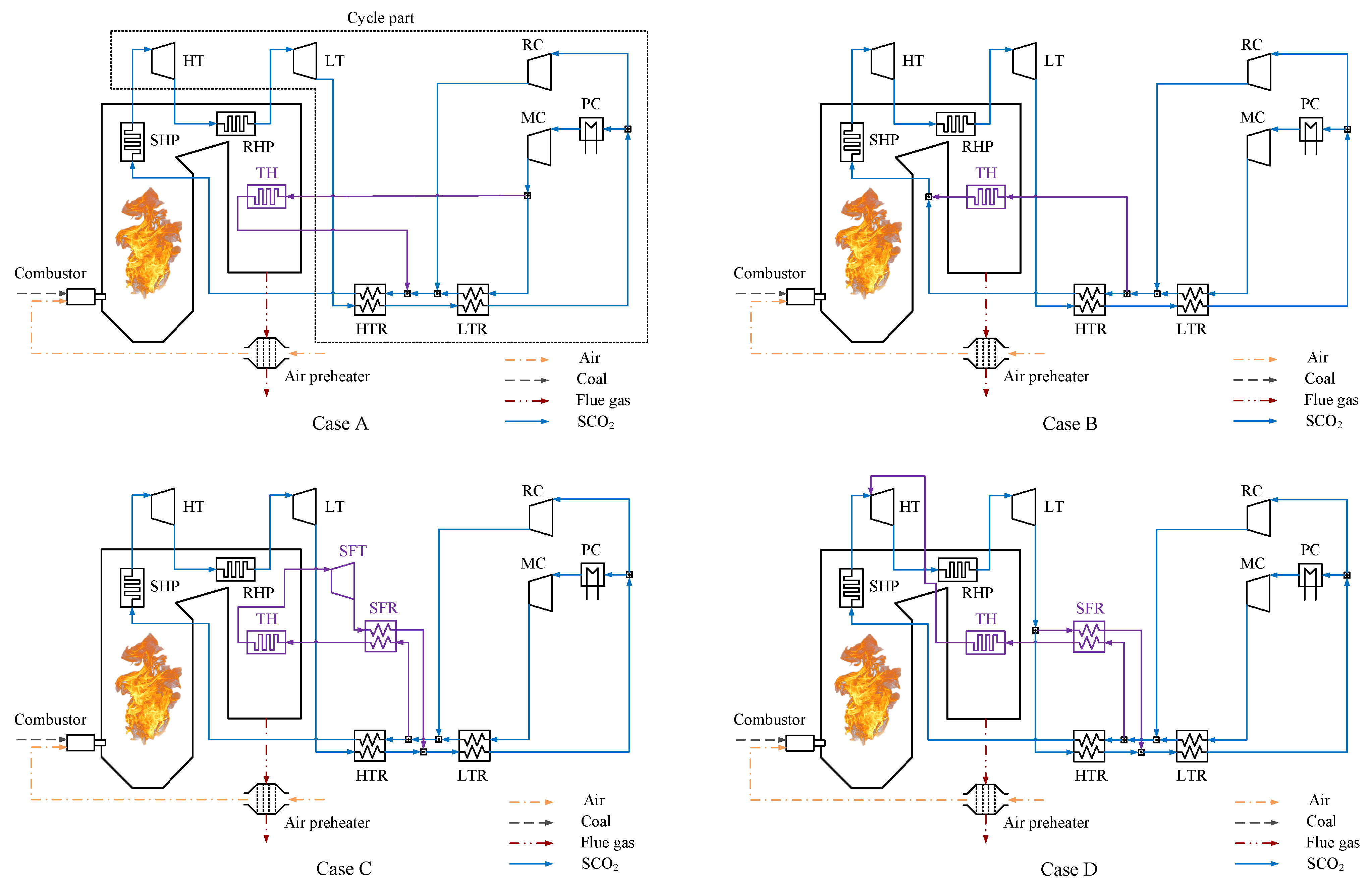
2.1. Typical System Layouts

Owing to the higher SCO₂ temperature before entering the boiler, the temperature of the tail flue gas is higher. Therefore, the extraction of tail flue gas energy is one of the critical concerns of SCPG systems [29]. It is necessary to split the lower temperature SCO₂ stream from the cycle part and utilize it to extract tail flue gas energy in the tail heater (TH). The basic SCPG system layout and its four extraction schemes constitute four typical system layouts, as shown in Figure 1. The components of the basic layout are shown in black. The extraction schemes are indicated in purple.

The basic layout consists of two parts: a boiler and a cycle. Specifically, the boiler includes heating surfaces, an air preheater, and a combustor. The heating surfaces consist of the superheat part (SHP) and reheat part (RHP). The SCO₂ recompression cycle is adopted as the cycle part. It includes two compressors: a main compressor (MC) and a recompressor (RC), two turbines: a low-pressure turbine (LT) and a high-pressure turbine (HT), two recuperators: a low-temperature recuperator (LTR) and a high-temperature recuperator (HTR), and a precooler (PC). The cycle process is described as follows. The superheated SCO₂ is expanded in the HT and is then sent to the RHP to be reheated. After being expanded in the LT, it enters the recuperation system to preheat the cold side stream and is then split into two streams. The main stream is allowed to enter the PC to release waste heat. After being compressed in the MC, it passes successively through the recuperation system and boiler to receive energy from the hot side stream and flue gas. The other stream is compressed in the RC, after which it is mixed into the cold side outlet of LTR.

Among the four extraction schemes, the reason behind choosing the former two is that they are representative heat absorption schemes using a direct split, whereas the reason for the latter two schemes is that they are representative heat absorption schemes based on a composite cycle. Their detailed explanations are as follows:

Case A (LTR parallel scheme): This scheme was adopted in Refs. [25,29]. The split path is parallel to the cold side of the LTR. Specifically, the stream is split from the outlet of the MC and mixed into the cold side outlet of the LTR.

Case B (HTR parallel scheme): This scheme was adopted in Refs. [25,30]. The split path is parallel to the cold side of the HTR. In particular, the stream is split from the cold side outlet of LTR and mixed into that of the HTR.

Case C (Top-bottom scheme): This scheme was proposed by Sun et al. according to the energy cascade utilization principle [31]. The stream is split from the cold side outlet of the LTR to form the bottom cycle to absorb the energy of the tail flue gas. The split flow turbine (SFT) and split flow recuperator (SFR) of the bottom cycle are independent of the top cycle. The heated stream is expanded in the SFT and is then mixed into the hot side outlet of the HTR after recuperation in the SFR.

Case D (Overlap scheme): This was proposed by Sun et al. according to the energy overlap utilization principle [32]. In contrast to Case C, the stream of the bottom cycle absorbs not only the energy of the tail flue gas but also the energy of the higher temperature flue gas. Therefore, the stream of the bottom cycle is heated to a higher temperature, and it shares turbines with the top cycle. The other parts are identical to those in Case C.

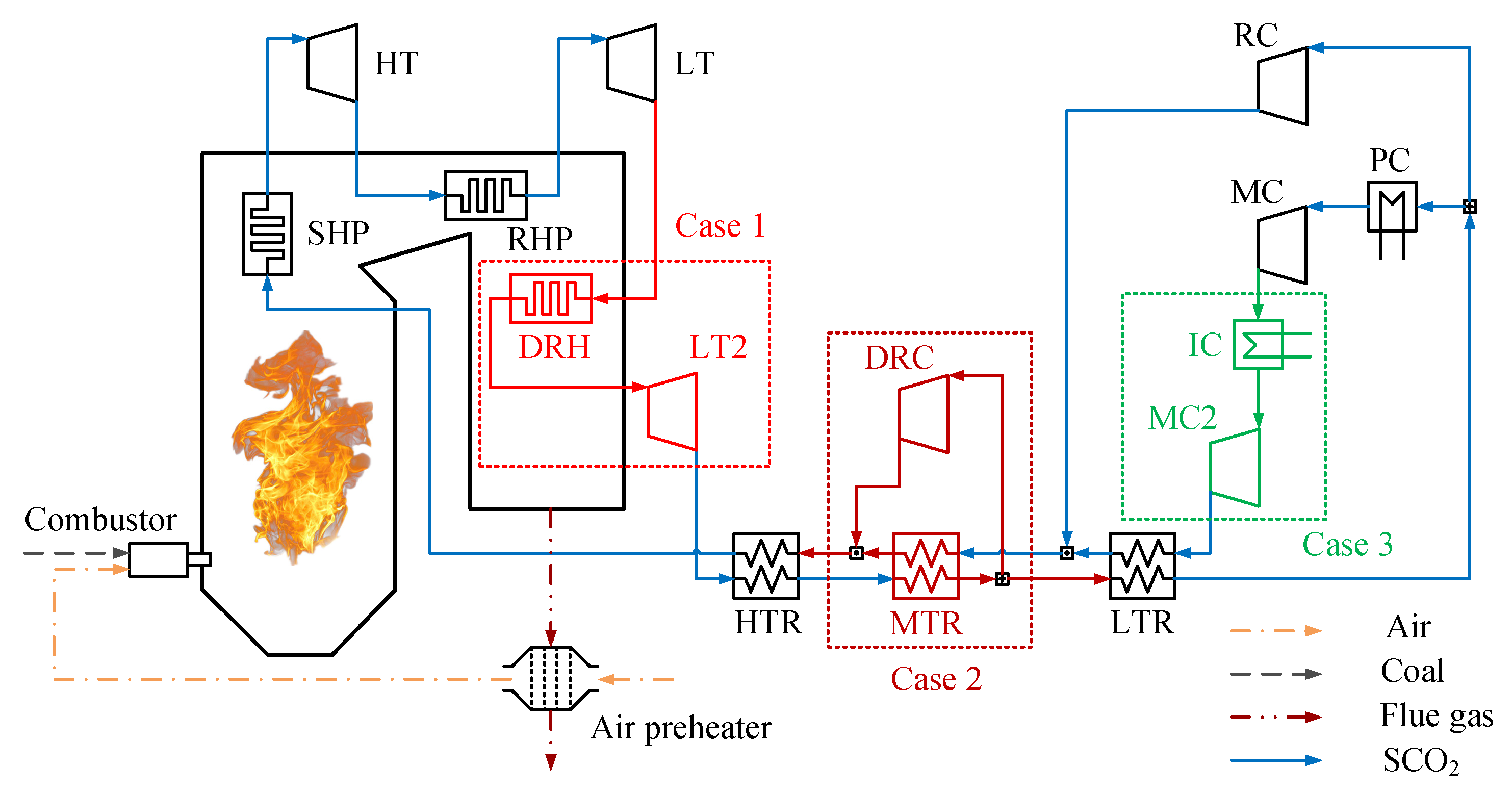
2.2. Improved System Layouts

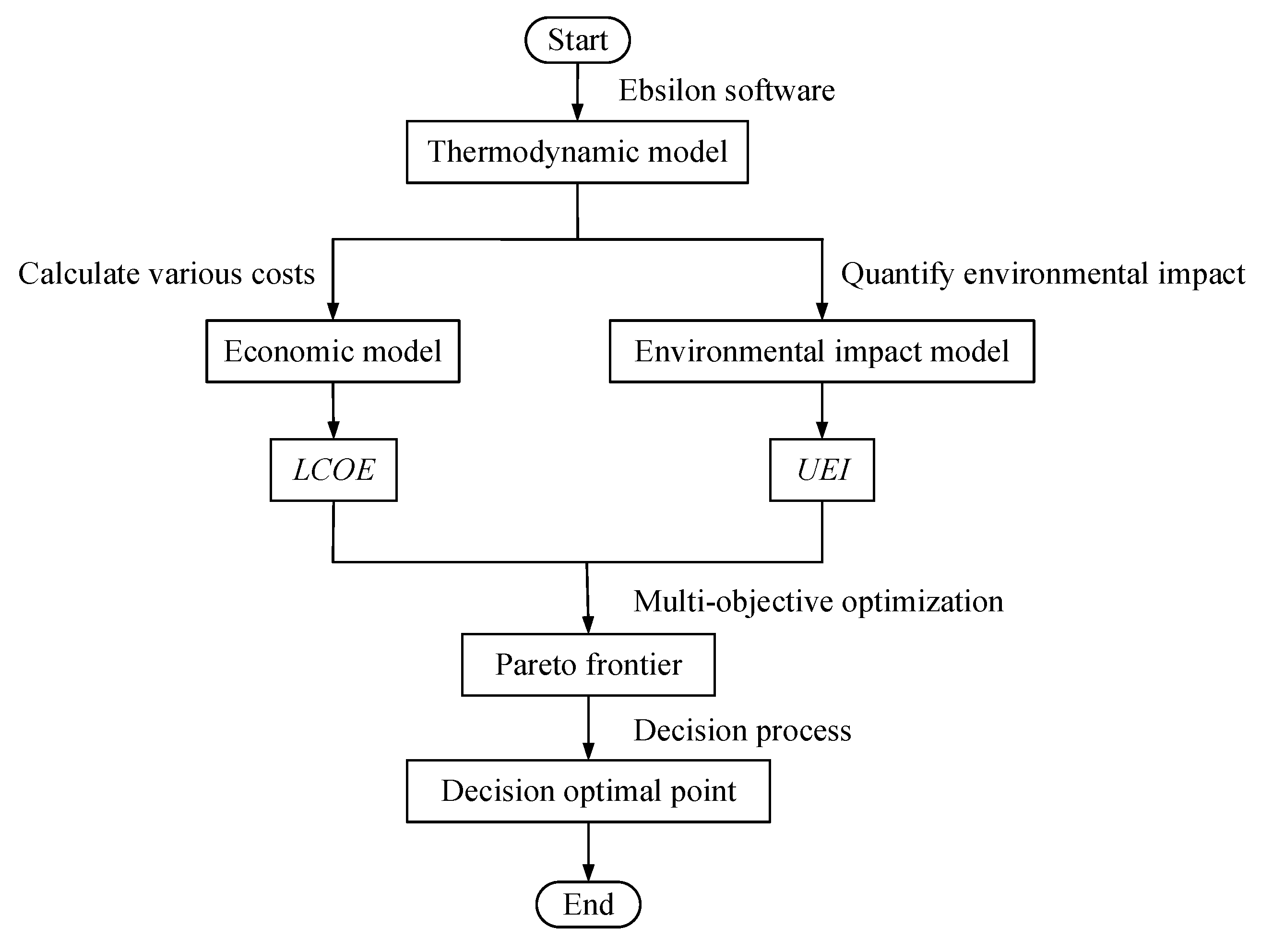
Based on the basic layout, three improved schemes are introduced to constitute three improved system layouts, as shown in Figure 2. The reason behind choosing them is that they are representative schemes for system efficiency improvement. These schemes target the expansion, recuperation, and compression processes of the system, respectively. The components of the basic layout are shown in black. The three improved schemes are indicated in other different colors. Their corresponding detailed explanations are as follows:

Case 1 (Double reheat scheme): The expanded stream in the LT is heated in a double reheater (DRH) and is then expanded in the LT2 to generate additional power. The average endothermic temperature of the SCO₂ in the boiler is increased, and thus the system efficiency is increased compared with the basic layout.

Case 2 (Double recompression scheme): This scheme was first proposed by Moisseytsev [33]. Similar to the recompression scheme, a medium-temperature recuperator (MTR) is introduced. The stream of the hot side outlet of the MTR is split to be compressed in a double recompressor (DRC) and is then mixed into the cold side outlet of the MTR. The heat transfer temperature difference of the recuperation system is decreased, and thus the system efficiency is increased compared with the basic layout.

Case 3 (Intercooling scheme): The compressed stream in the MC is cooled in the intercooler (IC) and is then compressed in the MC2 to the maximum pressure of the system. The total power consumption of compressors is decreased, and thus the system efficiency is increased compared with the basic layout.

Figure 2. The basic layout coupled with three improved schemes: (Case 1) Double reheat scheme. (Case 2) Double recompression scheme. (Case 3) Intercooling scheme.

Figure 2. The basic layout coupled with three improved schemes: (Case 1) Double reheat scheme. (Case 2) Double recompression scheme. (Case 3) Intercooling scheme.

3. Methodology

A logic flowchart of this section is shown in Figure 3. First, a thermodynamic model of the SCPG system is established using Ebsilon 13.02 software [34]. Second, based on this model, an economic and an environmental impact model are built by calculating various costs and quantifying the environmental impact of the system, respectively. The two objectives, namely, the levelized cost of electricity (LCOE) and the ultimate environmental impact (UEI) are obtained from the above models. Subsequently, multi-objective optimization for these two objectives is implemented to obtain the Pareto frontier. Finally, a decision process is conducted to find the decision optimal point from the Pareto frontier.

3.1. Thermodynamic Model

In this study, Ebsilon is employed to establish a thermodynamic model of the SCPG system. Because the corresponding codes are invisible to the users, it is necessary to verify the accuracy of this software. The simulation results of the entire system provided in Ref. [29] are used as a reference. In Ebsilon, the same model and input parameters as the above literature are applied. The comparison between present results and literature results is listed in

Table 1. The comparison between present results and literature results.

Items	Literature Results	Present Results	Errors
Cycle part
Heat transfer of recuperator (MW)	3822.59	3821.73	−0.02%
Power output of turbine (MW)	1359.81	1355.53	−0.31%
Power consumption of compressor (MW)	359.81	355.53	−1.19%
Heat release of cooler (MW)	952.51	949.63	−0.30%
Efficiency of cycle (%)	51.22	51.29	0.14%
Boiler part
Heat transfer to cycle part (MW)	1952.51	1949.63	−0.15%
Heat transfer of flue gas cooler (MW)	58.83	58.62	−0.35%
Heat loss of exhaust flue gas (MW)	118.02	117.58	−0.38%
Mass flow of coal (t/h)	317.54	315.85	−0.53%
Efficiency of boiler (%)	94.43	94.79	0.38%

. It can be seen that the errors are within a reasonable range, and thus the model established in Ebsilon is dependable.

In Ebsilon, the mass flow rate ($\dot{m}$), enthalpy (h), and composition of the flue gas are calculated according to the coal properties using an in-built function. This function can be expressed as Equation (1), the code of which is invisible to users.

$${\dot{m}}_{\mathrm{fg}},h_{\mathrm{fg}},M{F}_Y=f(X_{\mathrm{ar}}, \mathrm{LHV})$$

(1)

where MF_Y is the mass fraction of matter Y; X represents the coal elements, such as C, H, O, and so on; LHV is the low heat value of the coal; subscript fg represents the flue gas; subscript Y represents the combustion products of coal, such as CO₂, SO₂, NO_x, and so on; subscript ar represents the as-received basis. The as-received basis is a benchmark, which stipulates selecting the actually received fuel when measuring its elemental composition. The properties of the selected coal samples are provided in

Table 2. The properties of selected coal [29].

Car (%)	Har (%)	Oar (%)	Sar (%)	Nar (%)	Mar (%)	Aar (%)	LHV (kJ/kg)
61.70	3.67	8.56	0.60	1.12	15.55	8.80	23,442

.

Furthermore, the physical and thermodynamic properties of matters in Ebsilon are obtained from the standard reference database of the National Institute of Standards and Technology (NIST) [35]. Before establishing the system model, the following assumptions and considerations are formed.

• The studied system is established as a steady state model.
• The change of mechanical energy of working fluid is not considered.
• The heat release from the cycle part to the environment can be neglected.
• Except for the two streams at the outlet of the DRC and the cold side outlet of the MTR in Case 2, the two streams maintain identical temperatures before they are mixed [31].
• For the boiler model, the exhaust flue gas loss and ash thermophysical loss are obtained from the simulated results. All other losses are set to 1.2% [36].
• The pressure loss of the flue gas in the boiler is ignored [37].

The modeling process in Ebsilon involves selecting each component from the module library, connecting them using pipelines, setting input parameters, and performing simulations. The essence of the simulation is to solve the equation set generated from the energy equilibrium equations of all components. The energy equilibrium equations for the main components are presented in

Table 3. Energy equilibrium equations of main components.

Components	Energy Equilibrium Equations a
Boiler heating surface	${\dot{m}}_{\mathrm{fg}}\cdot (h_{\mathrm{fg},\mathrm{in}}-h_{\mathrm{fg},\mathrm{out}})={\dot{m}}_{{\mathrm{SCO}}_2}\cdot (h_{{\mathrm{SCO}}_2,\mathrm{out}}-h_{{\mathrm{SCO}}_2,\mathrm{in}})$
Recuperator	${\dot{m}}_{\mathrm{hot}}\cdot (h_{\mathrm{hot},\mathrm{in}}-h_{\mathrm{hot},\mathrm{out}})={\dot{m}}_{\mathrm{cold}}\cdot (h_{\mathrm{cold},\mathrm{out}}-h_{\mathrm{cold},\mathrm{in}})$
Turbine	${\dot{W}}_{\mathrm{t}}={\dot{m}}_{\mathrm{t}}\cdot (h_{\mathrm{t},\mathrm{in}}-h_{\mathrm{t},\mathrm{out}})$
Compressor	${\dot{W}}_{\mathrm{c}}={\dot{m}}_{\mathrm{c}}\cdot (h_{\mathrm{c},\mathrm{out}}-h_{\mathrm{c},\mathrm{in}})$
Precooler	${\dot{Q}}_{\mathrm{p}}={\dot{m}}_{\mathrm{p}}\cdot (h_{\mathrm{p},\mathrm{in}}-h_{\mathrm{p},\mathrm{out}})$

^a h—enthalpy, $\dot{m}$—mass flow rate, $\dot{W}$—power, $\dot{Q}$—heat rate. Subscript: fg—flue gas, t—turbine, c—compressor, p—precooler, in—inlet, out—outlet, hot—hot side, cold—cold side.

. The input parameters of the typical system models and those added owing to the improved schemes are listed in

Table 4. Input parameters of typical system models.

Parameters	Values
Maximum temperature of system (tmax)	600 °C a
Maximum pressure of system (pmax)	30 MPa a
Reheat pressure (prh)	16 MPa
Minimum pressure of system (pmin)	7.6 MPa b
Minimum temperature of system	32 °C a
Compressor isentropic efficiency	0.89 b
Turbine isentropic efficiency	0.93 a
Generator efficiency	0.99 a
Pinch temperature difference of recuperator	10 °C c
Pressure drop in components except for boiler	0.1 MPa b
Pressure drop in superheat part of boiler	0.6 MPa
Pressure drop in reheat part of boiler	0.25 MPa
Pressure drop in tail heater of boiler	0.1 MPa
Excess air coefficient	1.2 c
Split ratio to tail heater	0.1 d
Hot air temperature	340 °C
Exhaust temperature of flue gas	120 °C
Output electric power of system	300 MW

^a Ref. [38]. ^b Ref. [39]. ^c Ref. [29]. ^d Ref. [40].

and

Table 5. Added input parameters owing to the improved schemes.

Schemes	Parameters	Values
Double reheat	Inlet temperature of low-pressure turbine 2	600 °C a
	Inlet pressure of low-pressure turbine	20 MP a
	Inlet pressure of low-pressure turbine 2	13 MP a
	Pressure drop in double reheater of boiler	0.2 MP a
Double recompression	Second split ratio	0.15
Intercooling	Inlet pressure of intercooler (pic)	9.3 MP a
	Inlet temperature of intercooler	32 °C a

^a Ref. [38].

, respectively.

The system efficiency (η_sys) is calculated as

$${\eta }_{\mathrm{sys}}=\frac{{\dot{W}}_{\mathrm{ele}}}{{\dot{m}}_{\mathrm{coal}}\cdot \mathrm{LHV}}$$

(2)

where $\dot{W}$_ele is the output electric power of the system.

3.2. Economic Model

In this study, the total revenue requirement (TRR) method [41] is applied to calculate the annual levelized economic costs of the SCPG system. The cost values are baselined to USD₂₀₁₇ by the chemical engineering plant cost index. The levelized total revenue requirement (TRR_l) can be expressed as

$$TR{R}_l=C{C}_l+OM{C}_l+F{C}_l$$

(3)

The levelized carrying charges (CC_l) can be calculated as

$$C{C}_l=TCI\cdot CRF$$

(4)

where CRF is the capital recovery factor.

The total capital investment (TCI) includes direct and indirect costs, which can be calculated according to the total purchased equipment cost (PEC_tot).

$$TCI=\psi \cdot PE{C}_{\mathrm{tot}}$$

(5)

where ψ is the relation coefficient between TCI and PEC_tot.

The purchased equipment cost (PEC) of each component can be estimated by introducing the pressure correction coefficient (f_p) based on the National Energy Technology Laboratory (NETL) method [42]. The core equation is as follows:

$$PEC=\mathrm{a}\cdot C{P}^{\mathrm{b}}\cdot f_t\cdot f_p$$

(6)

where a and b are the fit coefficients according to the vendor quotes; CP is the characteristic parameter of the component; f_t is the temperature correction coefficient. A detailed explanation for calculating the PEC for each component is provided in Ref. [43].

The levelized operating and maintenance costs (OMC_l) and levelized fuel costs (FC_l) are calculated as:

$$OM{C}_l=OM{C}_0\cdot CELF$$

(7)

$$F{C}_l=F{C}_0\cdot CELF$$

(8)

where CELF is the constant escalation levelization factor.

The calculation of the CELF is as follows:

$$CELF=\frac{k(1-k^n)}{1-k}CRF$$

(9)

$$k=\frac{1+r_{\mathrm{n}}}{1+i_{\mathrm{e}}}$$

(10)

$$CRF=\frac{i_{\mathrm{e}}{(1+i_{\mathrm{e}})}^n}{{(1+i_{\mathrm{e}})}^n-1}$$

(11)

The first-year operating and maintenance costs (OMC) and fuel costs (FC) are calculated as [5]:

$$OM{C}_0={\phi }_{\mathrm{fix}}\cdot TCI+{\phi }_{\mathrm{var}}\cdot \tau \cdot {\dot{W}}_{\mathrm{ele}}$$

(12)

$$F{C}_0={\dot{m}}_{\mathrm{coal}}\cdot \mathrm{LHV}\cdot \tau \cdot c_{\mathrm{coal}}$$

(13)

The values of economic parameters are listed in

Table 6. The values of economic parameters.

Symbols	Economic Parameters	Values
n	system economic lifetime	20 year a
τ	annual operation hour	8000 h/year a
ie	annual effective interest rate	0.10 a
rn,OMC	annual nominal escalation rate of OMC	0.025 a
rn,FC	annual nominal escalation rate of FC	0.025 b
ψ	relation coefficient	1.3608 c
ccoal	coal price per unit of heat	4.09 USD/GJ d
φfix	fixed cost coefficient	0.015 e
φvar	variable cost coefficient	1.65 USD/MW e

^a Ref. [44]. ^b Ref. [45]. ^c Ref. [46]. ^d Ref. [47]. ^e Ref. [5].

.

The levelized system costs (SC_l) can be expressed as the sum of the levelized carrying charges and the levelized operating and maintenance costs.

$$S{C}_l=C{C}_l+OM{C}_l$$

(14)

Finally, the LCOE is calculated as follows:

$$LCOE=\frac{TR{R}_l}{\tau \cdot {\dot{W}}_{\mathrm{ele}}}$$

(15)

3.3. Environmental Impact Model

The calculation method for environmental impact adopted in the present study is a combination of the CML method [48] and the method proposed in Ref. [49]. The CML method is a method of assessing the impact of the system on the environment, which is developed by the Institute of Environmental Sciences of Leiden University. The considered environmental impact categories include global warming potential (GWP), acidification potential (AP), human toxicity potential (HTP), and dust pollution potential (DP). The pollutants considered in the system are CO₂, SO₂, NO_x, and dust. The removal efficiencies of SO₂, NO_x, and dust are 90% [50], 75% [51], and 99% [52], respectively.

The environmental impact of the ith category (EI_i) can be calculated as

$$E{I}_i={\displaystyle \sum _{j}A{E}_j\cdot C{F}_j}$$

(16)

where AE_j indicates annual emissions (kg/year) of the jth pollutant. CF_j indicates the characterization factor of the jth pollutant, which is listed in

Table 7. The values of characterization factor (CF).

Environmental Impact Categories	Units	Pollutants	CF
GWP	kg CO2-eq/kg	CO2	1 a
AP	kg SO2-eq/kg	SO2	1 a
		NOx	0.7 a
HTP	kg 1,4-DB-eq/kg	SO2	0.096 a
		NOx	1.2 a
DP	kg dust-eq/kg	dust	1 b

^a Ref. [53]. ^b Ref. [28].

. The unit of EI is the kilogram of pollutant equivalent per year (kg pollutant-eq/year).

The normalized environmental impact of the ith category (NEI_i) can be calculated as

$$NE{I}_i=E{I}_i/CE{I}_{90,i}$$

(17)

where CEI_90,i is the environmental impact per capita for China in 1990 of the ith category and is measured in kg pollutant-eq/year·p-eq. The unit of the NEI is the population equivalent (p-eq).

The ultimate environmental impact (UEI) can be calculated as

$$UEI={\displaystyle \sum _{i}NE{I}_i\cdot W{F}_i}$$

(18)

where the WF_i is the weight factor of the ith environmental impact category.

The values of the environmental impact per capita for China in 1990 (CEI₉₀) and the weight factor (WF) are obtained from Ref. [28] and are listed in

Table 8. The values of CEI₉₀ and WF.

Environmental Impact Categories	CEI90	WF
GWP	8700	0.83
AP	36	0.73
HTP	24.65	0.73
DP	18	0.61

.

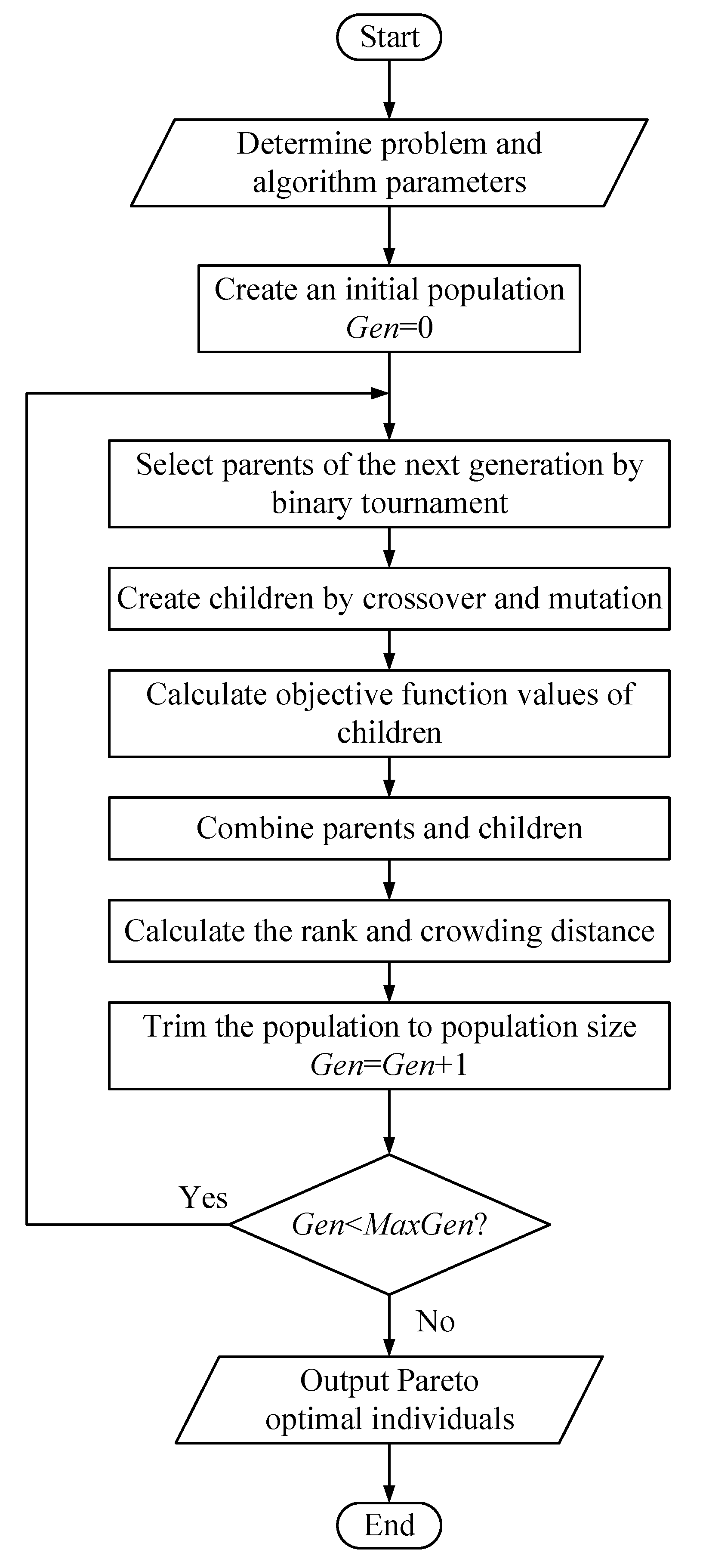
3.4. Multi-Objective Optimization Method

There are two types of methods for solving multi-objective optimization problems: the weighted summation method and the Pareto frontier method [28]. The weighted summation method transforms a multi-objective problem into a single-objective problem using the weighted summation of each objective, whereas the Pareto frontier method uses Pareto improvement to allow multiple objectives to reach a state. In this state, one objective cannot be improved without worsening the others. The final result will obtain the Pareto optimal point set, which is called the Pareto frontier.

The fast elitist non-dominated sorting genetic algorithm (NSGA-II) proposed by Deb et al. [54] belongs to the Pareto frontier method. In the present study, the gamultiobj algorithm in MATLAB R2014a software [55], which is a variant of NSGA-II, is adopted to perform multi-objective optimization. The biggest distinction between these two is the introduction of the Pareto fraction in the gamultiobj algorithm. This parameter is the ratio of the output Pareto optimal individuals to the population size. A flowchart of the gamultiobj algorithm is shown in Figure 4. First, the objectives, decision variables, and constraints of the problem are determined, and the algorithm parameters are set. Second, an initial population is created, the generation number (Gen) is marked as 0. Third, an iterative process is performed to achieve population evolution up to the maximum generation number (MaxGen), after which this iteration is stopped. Finally, the Pareto optimal individuals in the final population are obtained as the outputs. The values of the gamultiobj parameters in different sections are provided in

Table 9. The values of the gamultiobj parameters.

Parameters	Section 4.2	Section 4.4
Population size	100	100
MaxGen	1200	200
Pareto fraction	0.35 (Gen ≤ 1000)	0.35 (Gen ≤ 150)
	1 (Gen > 1000)	1 (Gen > 150)
Others	default	default

.

The purpose of increasing system efficiency is to save costs and protect the environment. Therefore, the goal of this study is to simultaneously minimize UEI and LCOE. The calculations for the two objectives are expressed in Equations (18) and (15). Five design parameters of the system are selected as the decision variables. These are expressed as follows:

$$\begin{array}{ll}\min .& UEI\left(t_{\max },p_{\max },p_{\mathrm{rh}},p_{\min },p_{\mathrm{ic}}\right) \&\\ & LCOE\left(t_{\max },p_{\max },p_{\mathrm{rh}},p_{\min },p_{\mathrm{ic}}\right)\end{array}$$

(19)

The range of decision variables and the corresponding constraints are as follows:

$$\{ \begin{array}{l}500 °\mathrm{C}<t_{\max }<700 °\mathrm{C}\hfill \\ 22 \mathrm{MPa}<p_{\max }<40 \mathrm{MPa}\hfill \\ 12 \mathrm{MPa}<p_{\mathrm{rh}}<21 \mathrm{MPa}\hfill \\ 7.4 \mathrm{MPa}<p_{\min }<10 \mathrm{MPa}\hfill \\ 7.4 \mathrm{MPa}<p_{\mathrm{ic}}<12 \mathrm{MPa}\hfill \\ p_{\min }<p_{\mathrm{ic}}\hfill \end{array}$$

(20)

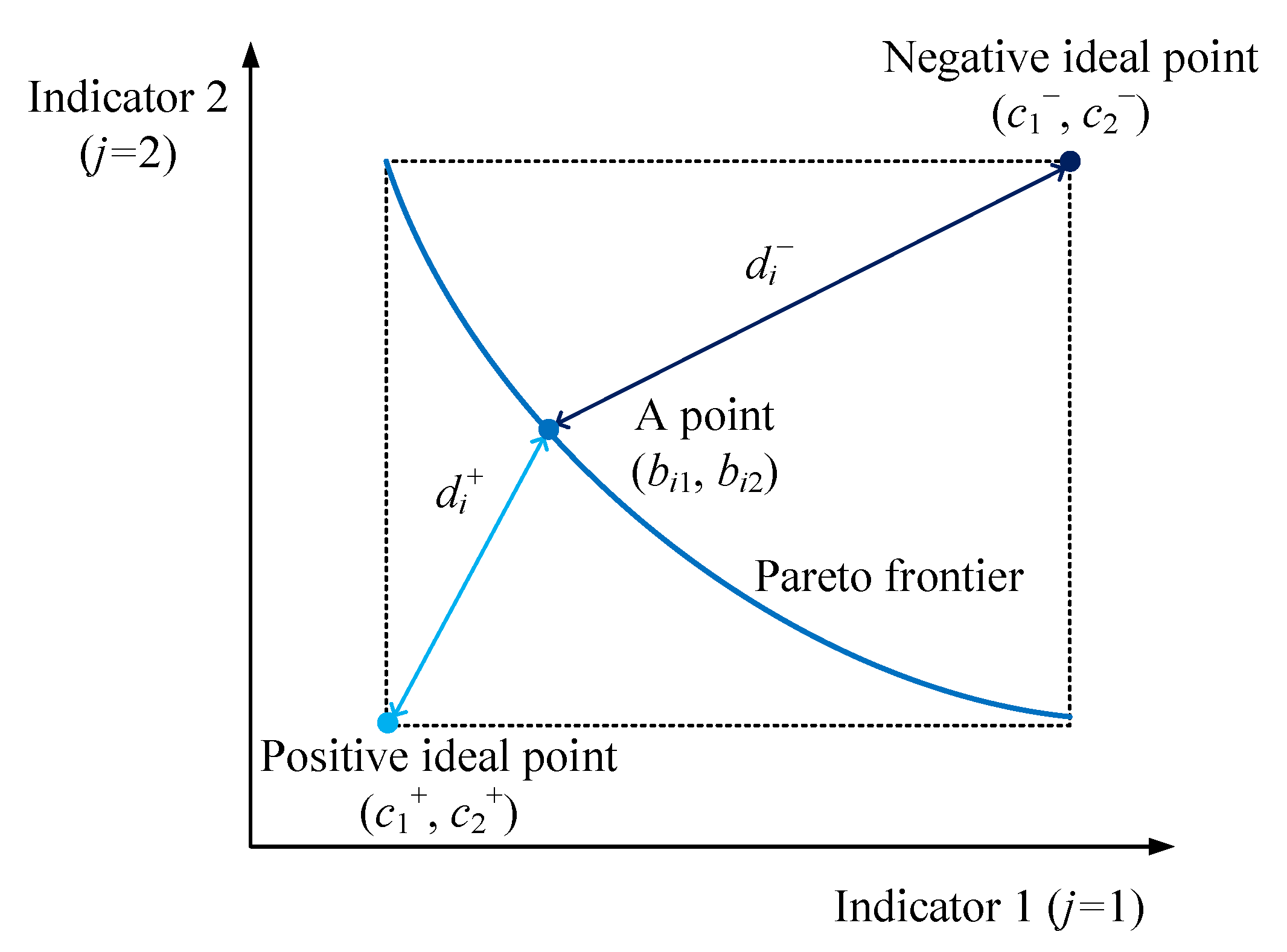
3.5. Decision Method

After obtaining the Pareto frontier, it is necessary to select a point from the Pareto frontier using a decision-making process. There are many decision methods, such as the ideal point method, principal component analysis method, and the analytic hierarchy process method. Among these, the ideal point method has the advantage of being simple and effective [56].

In this study, the technique for order preference by similarity to an ideal solution (TOPSIS) method proposed by Hwang and Yoon [57] is adopted. This method defines positive and negative ideal points, calculates their distances from each point, and ultimately searches for a point that is close to the positive ideal point and far from the negative ideal point. This point ensures a trade-off between multiple indicators and is called the decision optimal point (DOP). The steps of this method are detailed as follows [58].

For a decision-making problem, m candidates for competition and n indicators are involved in the evaluation, which can be represented as an m × n matrix, as shown in Equation (21).

$$\mathit{A}={(a_{ij})}_{m\times n}={\left[\begin{array}{cccc}{a}_{11}& a_{12}& \cdots & a_{1n}\\ a_{21}& a_{22}& \cdots & a_{2n}\\ ⋮& ⋮& \ddots & ⋮\\ a_{m1}& a_{m2}& \cdots & a_{mn}\end{array}\right]}_{m\times n}$$

(21)

where a_ij represents the value of the jth indicator for the ith candidate. Hereafter, i = 1, 2, …, m; j = 1, 2, …, n.

First, a normalization from matrix A to matrix B is conducted to eliminate the dimensional effect of the different indicators, as shown in Equation (22).

$$\mathit{B}={(b_{ij})}_{m\times n} , b_{ij}=\frac{a_{ij}}{\sqrt{ {\displaystyle \sum _{i=1}^m{a}_{ij}{}^2}}}$$

(22)

where b_ij represents the dimensionless value of the jth indicator for the ith candidate.

Second, the positive and negative ideal points are confirmed. The positive ideal point ($c_j^{+}$) is where each indicator reaches the maximum (for benefit attribute) or minimum (for cost attribute) of all points. The negative ideal point ($c_j^{-}$) is where each indicator reaches the minimum (for benefit attribute) or maximum (for cost attribute) of all points. These two points are expressed as follows:

$$c_j^{+}=\{\begin{array}{l}\underset{i}{\max }{b}_{ij} \mathrm{if} j \mathrm{is} \mathrm{benefit} \mathrm{attribute}\hfill \\ \underset{i}{\min }{b}_{ij} \mathrm{if} j \mathrm{is} \cos \mathrm{t} \mathrm{attribute}\hfill \end{array}$$

(23)

$$c_j^{-}=\{\begin{array}{l}\underset{i}{\min }{b}_{ij} \mathrm{if} j \mathrm{is} \mathrm{benefit} \mathrm{attribute}\hfill \\ \underset{i}{\max }{b}_{ij} \mathrm{if} j \mathrm{is} \cos \mathrm{t} \mathrm{attribute}\hfill \end{array}$$

(24)

Third, in the n-dimension space, the Euclidean distance between each point and the positive ideal point ($d_i^{+}$) and that between each point and the negative ideal point ($d_i^{-}$) are calculated as follows:

$$d_i{}^{+}=\sqrt{ {\displaystyle \sum _{j=1}^n{(b_{ij}-c_j{}^{+})}^2}}$$

(25)

$$d_i{}^{-}=\sqrt{ {\displaystyle \sum _{j=1}^n{(b_{ij}-c_j{}^{-})}^2}}$$

(26)

For a graphical display, only two indicators with cost attributes are assumed. Based on this assumption, a diagram of the second and third steps of the TOPSIS method is shown in Figure 5.

Fourth, the closeness coefficient (CLC_i) is used to weigh the relative distance between each point and the two ideal points, which can reflect the degree of relative closeness to the positive ideal point, and is expressed as follows:

$$CL{C}_i=\frac{d_i{}^{-}}{d_i{}^{+}+d_i{}^{-}}$$

(27)

Finally, all points are sorted in descending order according to the CLC_i. The point with the maximum CLC_i is considered as the decision optimal point.

4. Results and Discussion

4.1. Comparison of Different Layouts

In this section, under the objectives of UEI and LCOE, the comparisons of four typical layouts and three improved layouts are conducted to select the optimal layout with the best comprehensive performance.

4.1.1. Comparison of Typical Layouts

Figure 6a shows a comparison of the UEI and LCOE for the four typical layouts. Both objectives are cost attributes, and thus the closer a point is to the bottom left, the better the comprehensive performance it provides. Comparisons of the thermodynamic and economic parameters for the four typical layouts are shown in Figure 6b and

Table 10. Comparison of system efficiency (η_sys) and purchased equipment cost (PEC) for four typical layouts.

Items	Case A	Case B	Case C	Case D
Efficiency (%)
ηsys	46.20	47.85	47.19	47.89
PEC of identical components (USD)
Boiler	1.43 × 108	1.39 × 108	1.40 × 108	1.39 × 108
High-pressure turbine (HT)	5.67 × 106	5.77 × 106	5.55 × 106	5.78 × 106
Low-pressure turbine (LT)	4.76 × 106	4.85 × 106	4.64 × 106	4.84 × 106
Main compressor (MC)	8.36 × 106	8.13 × 106	8.22 × 106	8.12 × 106
Recompressor (RC)	8.14 × 106	9.14 × 106	9.25 × 106	9.13 × 106
High-temperature recuperator (HTR)	2.87 × 107	4.66 × 107	2.78 × 107	2.72 × 107
Low-temperature recuperator (LTR)	3.39 × 107	3.47 × 107	3.55 × 107	3.47 × 107
Precooler (PC)	5.26 × 106	4.88 × 106	5.03 × 106	4.87 × 106
Generator	2.46 × 106	2.46 × 106	2.46 × 106	2.46 × 106
PEC of added components (USD)
Split flow recuperator (SFR)	-	-	2.57 × 106	5.18 × 106
Split flow turbine (SFT)	-	-	1.76 × 106	-

.

From Figure 6a, it can be observed that Case D has the lowest UEI and LCOE. This is because it has the highest η_sys and the second-lowest SC_l. The reason for its highest η_sys is that it has the highest heat absorption quantity of tail flue gas. Case A has the highest UEI and LCOE values. This is mainly because it has the lowest η_sys, which leads to the highest FC_l. The reason for its lowest η_sys is that it has the lowest heat absorption quantity of tail flue gas. Although SC_l is the lowest, the LCOE is the highest owing to its large FC_l.

Cases B and C have different advantages. Compared with Case C, Case B has a lower UEI. This is because its η_sys is higher than that of Case C, which is consistent with the result in Ref. [25]. Compared with Case B, Case C has a lower LCOE mainly because of the drastic decrease in the HTR cost, which reduces its SC_l. Specifically, the introduction of the SFR shares the huge heat transfer of the HTR, which increases the heat transfer temperature difference, ultimately causing a drastic decrease in the HTR cost. Compared with Case C, the UEI of Case B decreases by 1.39% at the expense of increasing the LCOE by 0.74%. The benefit outweighs the expense. Hence, the comprehensive performance of Case B is better than that of Case C.

In conclusion, the comprehensive performance ranks of the typical layouts in descending order are Case D, Case B, Case C, and Case A. Therefore, Case D is selected as the system to be improved upon in the next section. Moreover, in the comparison of Cases B and D, the introduction of SFR increases the heat transfer temperature difference, and the SC_l is reduced while the η_sys is increased. Therefore, it is feasible to increase the heat transfer temperature difference by introducing an SFR.

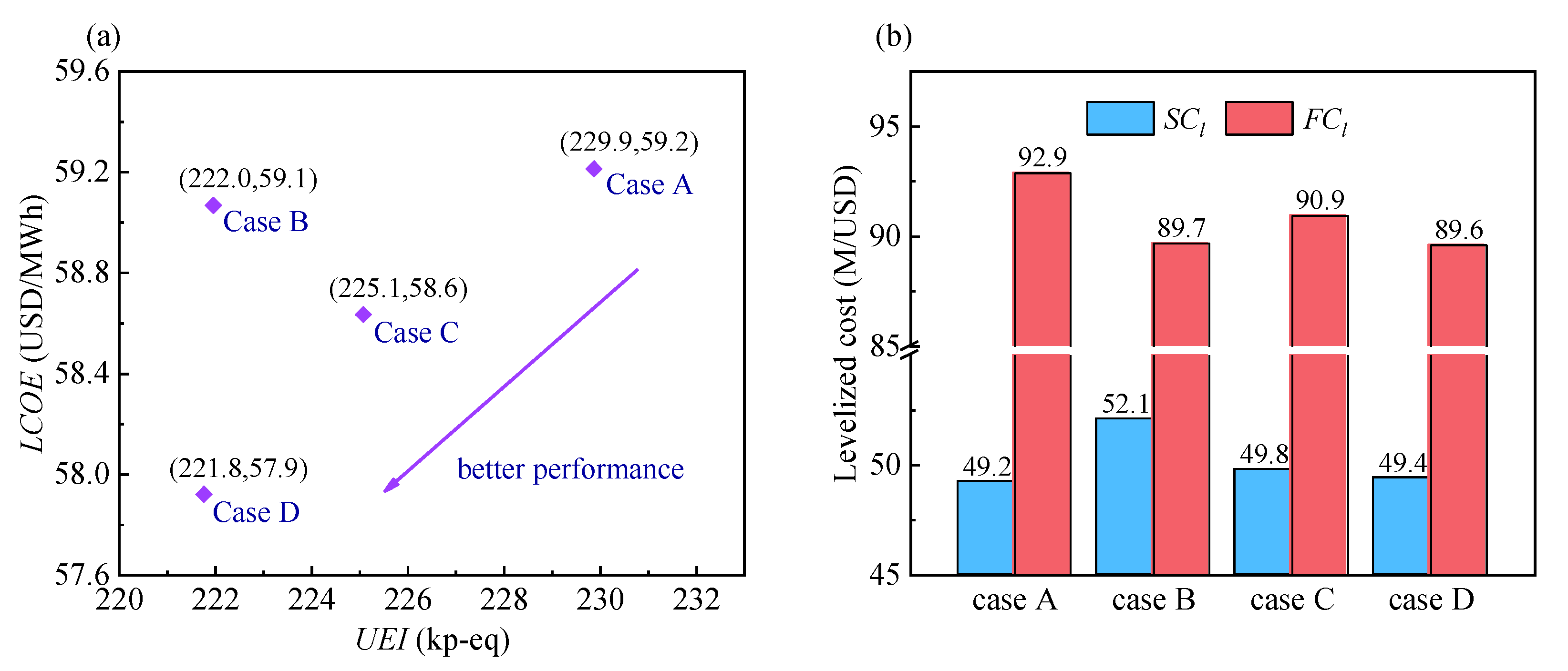
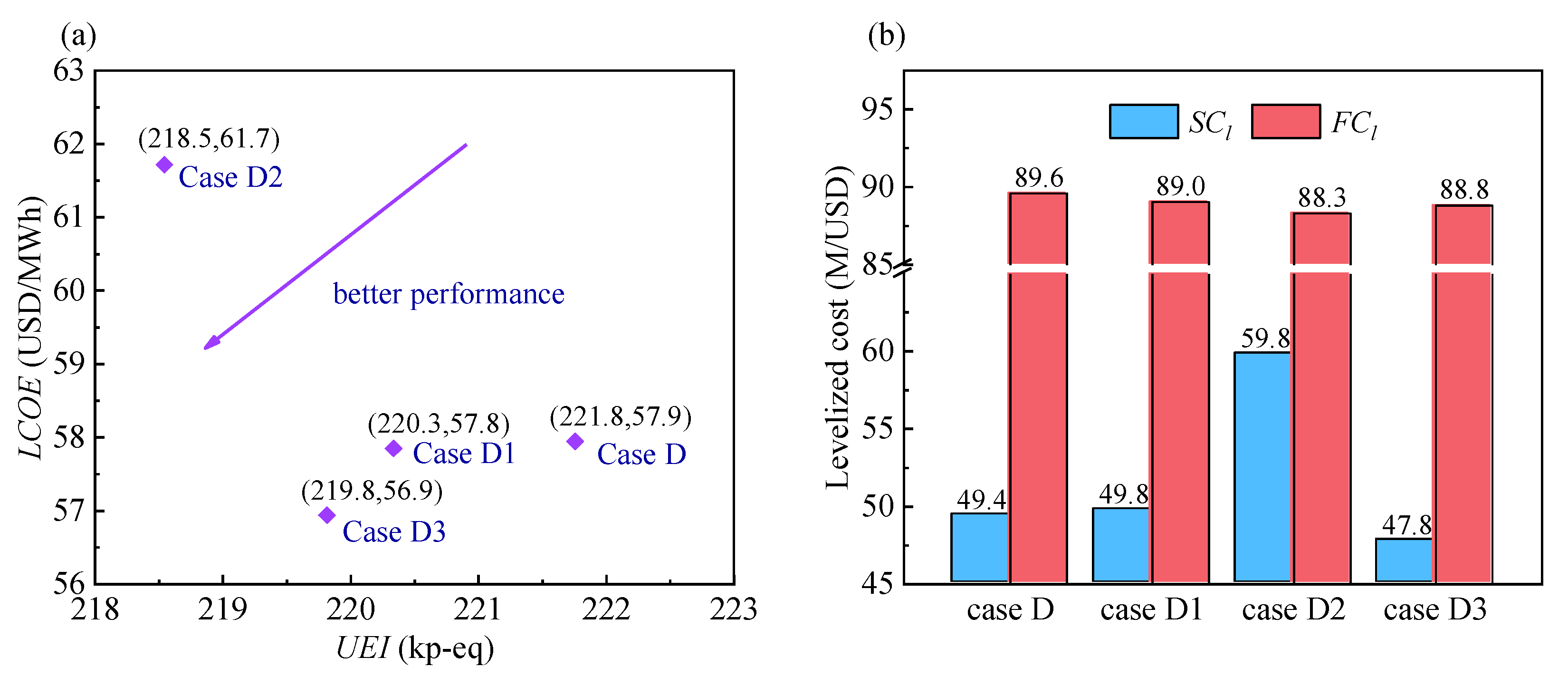
4.1.2. Comparison of Improved Layouts

Figure 7a compares the UEI and LCOE for the three improved layouts. Comparisons of the thermodynamic and economic parameters for these layouts are presented in Figure 7b and

Table 11. Comparison of system efficiency (η_sys) and purchased equipment cost (PEC) for three improved layouts.

Items	Case D	Case D1	Case D2	Case D3
Efficiency (%)
ηsys	47.89	48.20	48.60	48.32
PEC of identical components (USD)
Boiler	1.39 × 108	1.38 × 108	1.37 × 108	1.38 × 108
HT	5.78 × 106	4.51 × 106	6.21 × 106	5.64 × 106
LT	4.84 × 106	4.01 × 106	5.19 × 106	4.72 × 106
MC	8.12 × 106	8.08 × 106	8.03 × 106	2.32 × 106
RC	9.13 × 106	9.09 × 106	9.03 × 106	8.62 × 106
HTR	2.72 × 107	2.85 × 107	1.64 × 107	2.61 × 107
LTR	3.47 × 107	3.43 × 107	3.39 × 107	2.49 × 107
PC	4.87 × 106	4.80 × 106	4.71 × 106	5.01 × 106
Generator	2.46 × 106	2.46 × 106	2.46 × 106	2.46 × 106
SFR	5.18 × 106	5.43 × 106	3.13 × 106	4.98 × 106
PEC of added components (USD)
LT2	-	3.60 × 106	-	-
Medium-temperature recuperator (MTR)	-	-	6.27 × 107	-
Double recompressor (DRC) or MC2	-	-	8.50 × 106	7.25 × 106
Intercooler (IC)	-	-	-	2.22 × 106

.

In comparison with Case D, the UEI and LCOE are reduced in Cases D1 and D3. Furthermore, the reductions in Case D3 are more prominent than those in Case D1. In particular, in Case D1, the double reheat process increases the average endothermic temperature of SCO₂, the η_sys is improved, and the UEI is ultimately reduced. The introduction of LT2 increases the SC_l. In Case D3, the intercooling process decreases the MC power consumption. The coal consumption decreases due to a constant output of electric power, which consequently decreases the UEI. Despite the increased number of components, the heat transfer quantity of the LTR is decreased, and the LTR cost is reduced. As a result, the SC_l is reduced.

For Case D2, the second split process reduces the mass flow rate of exothermic SCO₂, which consequently reduces the total heat release quantity in the PC. Meanwhile, the heat transfer temperature difference of the recuperation system decreases owing to the double recompression process. However, the corresponding costs of the recuperation system increase. Compared with Case D, the UEI decreases by 1.45% at the expense of increasing the LCOE by 6.55%. In other words, it pays high expense while gaining low benefit. Hence, the comprehensive performance of Case D2 is worse than that of Case D, which also implies that the heat transfer temperature difference of the regenerator is not necessarily the smaller the better.

In conclusion, the comprehensive performance ranks of the improved layouts in descending order are Case D3, Case D1, Case D, and Case D2. Therefore, Case D3 is the optimal layout and is selected as the system to be optimized in the subsequent section.

4.2. Analysis of Multi-Objective Optimization Results

Multi-objective optimization is implemented to obtain the Pareto frontier of the layout of Case D3. Subsequently, the characteristics and correlations of all the design parameter points in the Pareto frontier are explored.

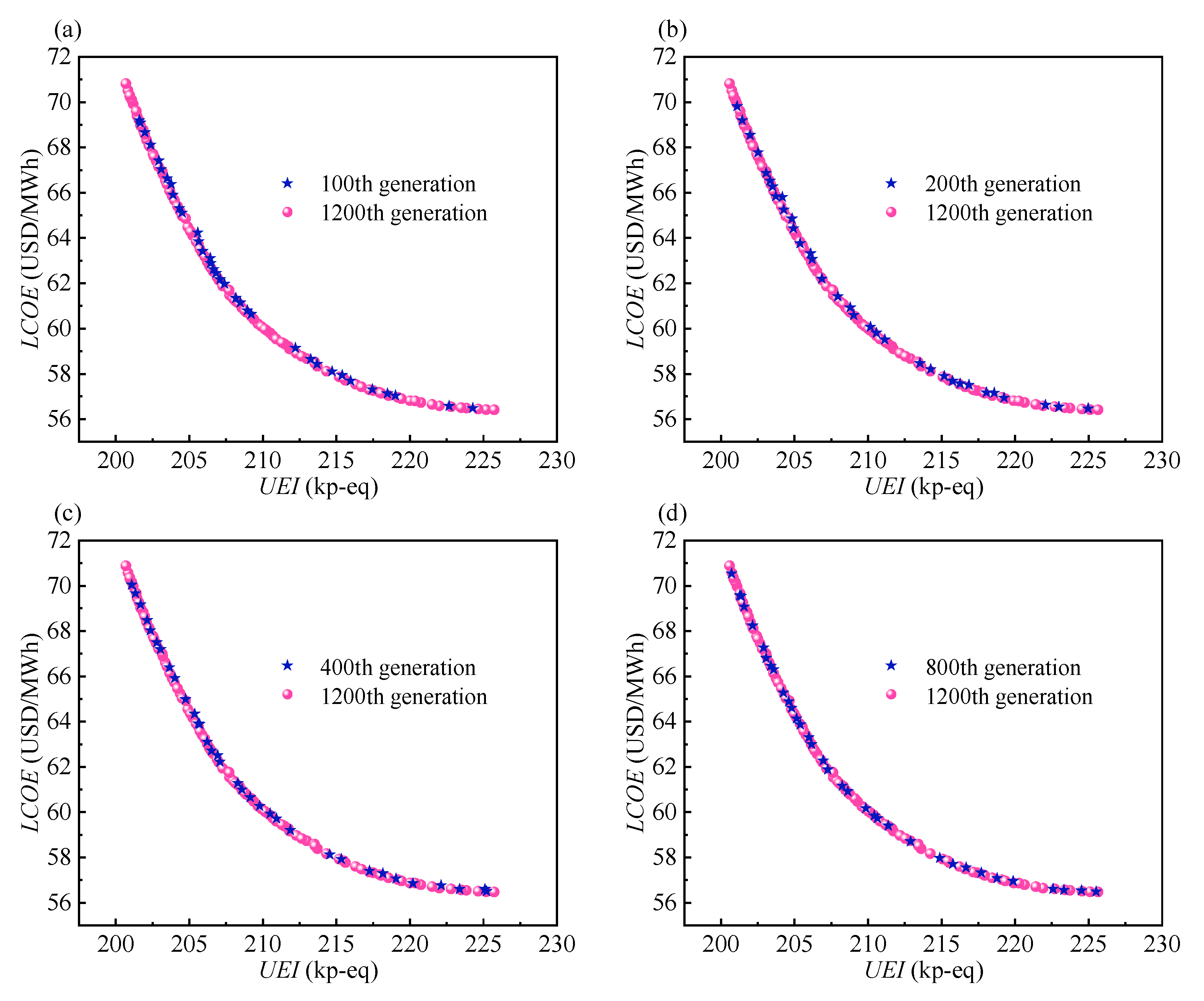
4.2.1. Evolution Process of Pareto Frontier

Figure 8 shows the Pareto frontier with the objectives of the UEI and LCOE for the different generations. The Pareto frontier of the 1200th generation is the final result and is used as a reference for other generations to reflect its evolution process. The reason for the higher number of points in the 1200th generation is the increased Pareto fraction after the 1000th generation.

From Figure 8, it can be observed that the Pareto frontier of the 100th generation is close to that of the 1200th generation, which means that the evolution process is fast. As the number of generations increases further, the two endpoints of the Pareto frontier appear in the trend of the extension. From the 100th to the 200th generation, the speed of extension is fast, after which it slows down. By the 200th generation, the two endpoints are close to the final endpoints of the 1200th generation. Hence, the 200th generation reflects the profile of the 1200th generation, which explains why the MaxGen is set to 200 in the sensitivity analysis. Moreover, the final result indicates that the two objectives conflict with each other. In other words, the benefit of one objective comes at the expense of the other. This indicates that each point is a candidate, and thus it is necessary to perform a characteristic analysis for all points.

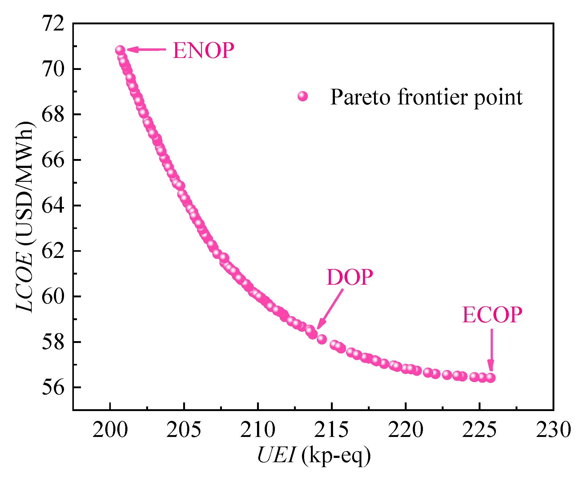
4.2.2. Characteristic Analysis of Pareto Optimal Points

In this section, the variations of the thermodynamic and economic parameters corresponding to the Pareto optimal points are presented to reflect the characteristics of all Pareto optimal points. The variations of the design parameters and system output parameters corresponding to the Pareto optimal points are shown in Figure 9 and Figure 10, respectively. The design parameters include the maximum temperature of the system (t_max), the maximum pressure of the system (p_max), the reheat pressure (p_rh), the minimum pressure of the system (p_min), and the inlet pressure of the intercooler (p_ic).

It can be seen from Figure 9a that the t_max and p_max tend to decrease with an increase in the UEI. It can be explained that high UEI values indicate that high efficiency is no longer needed. As a result, the maximum temperature/pressure of the system decreases. As shown in Figure 9b, the two pressure parameters p_rh and p_ic tend to decrease because of the decrease in the p_max. It is worth mentioning that the points of the p_rh and p_ic are concentrated and show an approximately linear decrease when the UEI is below 207 kp-eq. Above this value, their points become dispersed, which indicates that the correlations between them and the UEI decrease.

As shown in Figure 10a, the input heat rate of the boiler shows the largest variation with an increase in the UEI. The variations in the total power output of the turbines and the total power consumption of the compressors are identical because the output electric power of the system is set to a constant value of 300 MW. Referring to Figure 10b, the total recuperation rate and mass flow rate of SCO₂ increase with the increasing UEI. This can be explained by the fact that an increase in the input heat rate of the boiler requires more SCO₂ to absorb heat. Moreover, an increase in the mass flow rate leads to an increase in the total recuperation rate.

Figure 11 plots the variation of carrying charges (CC_l), operating and maintenance costs (OMC_l), and fuel costs (FC_l) corresponding to the Pareto optimal points. It can be seen that CC_l decreases with the increase in the UEI and that the curve tends to flatten gradually. Moreover, the FC_l values are larger than the CC_l values among all the UEI regions, while the variation of FC_l is less than that of CC_l. With the decrease in the UEI, the t_max increases. More expensive materials are needed to resist high temperatures, and thus the CC_l increases. An increase in the t_max will increase the η_sys and reduce the FC_l, but the increase in material costs is more prominent. Therefore, the variation of CC_l is larger than that of FC_l. In addition, the profile of CC_l is similar to that of the LCOE, which indicates that the variation of CC_l accounts for the main influence on the LCOE. Therefore, more attention should be focused on it.

Figure 12 displays the variation of purchased equipment cost (PEC) corresponding to Pareto optimal points, which is divided into two figures depending on whether the PEC is larger than 20 M/USD. As shown in Figure 12a, the PEC of the boiler shows the largest values and largest variation among the three components. Moreover, the profile of boiler PEC is similar to the profile of CC_l. These results indicate that the boiler PEC accounts for the main influence on CC_l. The variation of the boiler PEC is more apparent in the lower UEI region. This implies that as the UEI decreases, a higher boiler cost is required for reducing an identical UEI. Moreover, a UEI of 207 kp-eq splits the curve of the HTR into two parts. In the right part, the HTR PEC increases gently, whereas, in the left part, it shows a relatively rapid decline. A similar trend is visible in the curve of SFR PEC, as shown in Figure 12b. The reason for these trends is as follows: With the decrease in the UEI, the η_sys increases, the heat transfer quantity of these two components decreases, and thus the PEC decreases. When the UEI decreases below 207 kp-eq, the increase in the material costs caused by higher temperature becomes more prominent, and thus the PEC increases rapidly.

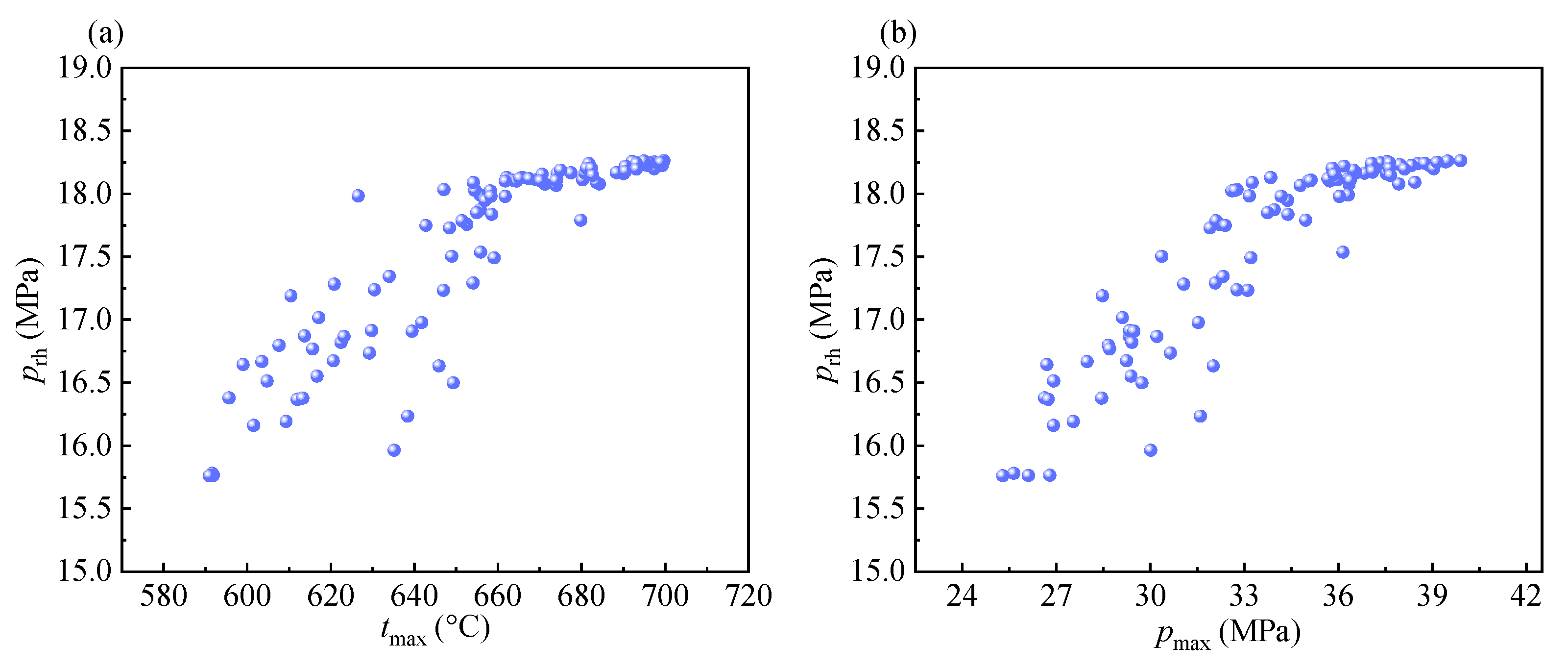
4.2.3. Correlation Analysis of Pareto Optimal Points

According to the analysis of Figure 9, a certain relation exists between the design parameters and the objective. Therefore, as proposed by Spearman in 1904, the Spearman correlation coefficient (ρ_s) [59], which could take values in the range of −1 and 1, is applied to quantify the relation. Here, positive and negative values denote positive and negative correlations, respectively. The larger the absolute value, the stronger the correlation.

Table 12. Spearman correlation coefficient among seven parameters.

Rank	Parameters	Values	Rank	Parameters	Values
1st	UEI and LCOE	−1.000	12th	pic and LCOE	0.909
2nd	tmax and LCOE	0.997	12th	pic and UEI	−0.909
2nd	tmax and UEI	−0.997	14th	tmax and pic	0.903
4th	pmax and LCOE	0.979	15th	pmax and pic	0.901
4th	pmax and UEI	−0.979	16th	prh and pmin	0.888
6th	tmax and pmax	0.966	17th	pmax and pmin	0.885
7th	prh and LCOE	0.947	18th	pmin and pic	0.885
7th	prh and UEI	−0.947	19th	pmin and LCOE	0.879
9th	tmax and prh	0.943	19th	pmin and UEI	−0.879
10th	pmax and prh	0.932	21st	tmax and pmin	0.870
11th	prh and pic	0.919

presents the ρ_s among the seven parameters (five design parameters and two objectives), which are sorted by absolute values in descending order. It can be seen that the ρ_s between the UEI and LCOE is −1, which indicates their completely monotonic negative correlation. The t_max and p_max show the 2nd and 4th strongest correlations, respectively, with the two objectives. This indicates that the t_max and p_max are the first and second most crucial parameters of the system, respectively. The t_max and p_max show the 6th strongest correlation with each other, and thus coordination between them is required in the parameter design process. In other words, their design values are determined together according to the relation between them.

Furthermore, relatively weaker correlations are observed between the p_rh and the two objectives, p_rh and t_max, and between the p_rh and p_max, which rank 7th, 9th, and 10th, respectively. These indicate that the p_rh is the third most crucial parameter of the system. In Figure 13, the relation between the p_rh and t_max, and that between p_rh and p_max are plotted as a scatter plot to visualize these relations. It can be observed that close correlations appear in the high-parameter region.

4.3. Comparison of Three Optimal Points

The decision optimal point (DOP) is obtained through the decision process, which is then compared with the environmental optimal point (ENOP) and economic optimal point (ECOP) to demonstrate its advantage. As shown in Figure 14, these three optimal points are marked in the Pareto frontier. It can be observed that a huge expense of UEI is required to reduce the LCOE around the ECOP. Moreover, the LCOE expense of reducing the UEI is high around the ENOP. The DOP lies between the ENOP and ECOP, which is a trade-off between the two objectives. The advantage of the DOP is that it simultaneously maintains lower environmental impact and economic costs.

The values of the five design parameters and two objectives corresponding to the three optimal points are listed in

Table 13. Comparison of three optimal points.

Points	tmax (°C)	pmax (MPa)	prh (MPa)	pmin (MPa)	pic (MPa)	UEI (kp-eq)	LCOE (USD/MWh)
DOP	635.3	30.08	15.95	7.602	9.216	213.8	58.29
ENOP	700.0	40.00	18.26	7.639	10.68	200.7	70.82
ECOP	591.1	25.35	15.74	7.596	8.738	225.8	56.37

. It can be seen that the maximum temperature/pressure of the system is 591 °C/25.4 MPa when the LCOE is the lowest. Moreover, the t_max and p_max reach the maximum values of the given boundary when the UEI is the lowest. For DOP, the maximum temperature/pressure of the system is found to be 635.3 °C/30.1 MPa. Compared with the ECOP, the UEI decreases by 5.3% at the expense of increasing the LCOE by 3.4%. Compared with the ENOP, the LCOE decreases by 17.7% at the expense of increasing the UEI by 6.5%. In other words, high benefits could be obtained at low expenses, and thus the DOP has a better comprehensive performance.

For further analysis of the DOP, the ingredient distributions of the UEI and LCOE are shown in Figure 15. The ingredient distributions of UEI include global warming potential (GWP), acidification potential (AP), human toxicity potential (HTP), and dust pollution potential (DP). As shown in Figure 15a, GWP contributes approximately 75% of the UEI, which is due to the massive emissions of CO₂ without the capture process. Therefore, the challenge of the SCPG system is to decrease CO₂ emissions. The second contribution is DP, which accounts for 9.83% of the UEI. Although the dust removal efficiency has reached 99%, its environmental impact continues to be higher than that of SO₂ and NO_x. Hence, dust emissions should also be considered seriously. Moreover, as shown in Figure 15b, FC_l accounts for more than half of the LCOE (61.73%), followed by CC_l (30.1%) and OMC_l (8.17%).

Finally, the basic layout coupled with overlap and intercooling schemes (Case D3) is determined to be the optimal layout. The decision optimal point (DOP) is determined to be the optimal design parameters. The Ebsilon model of this system is demonstrated in Figure 16.

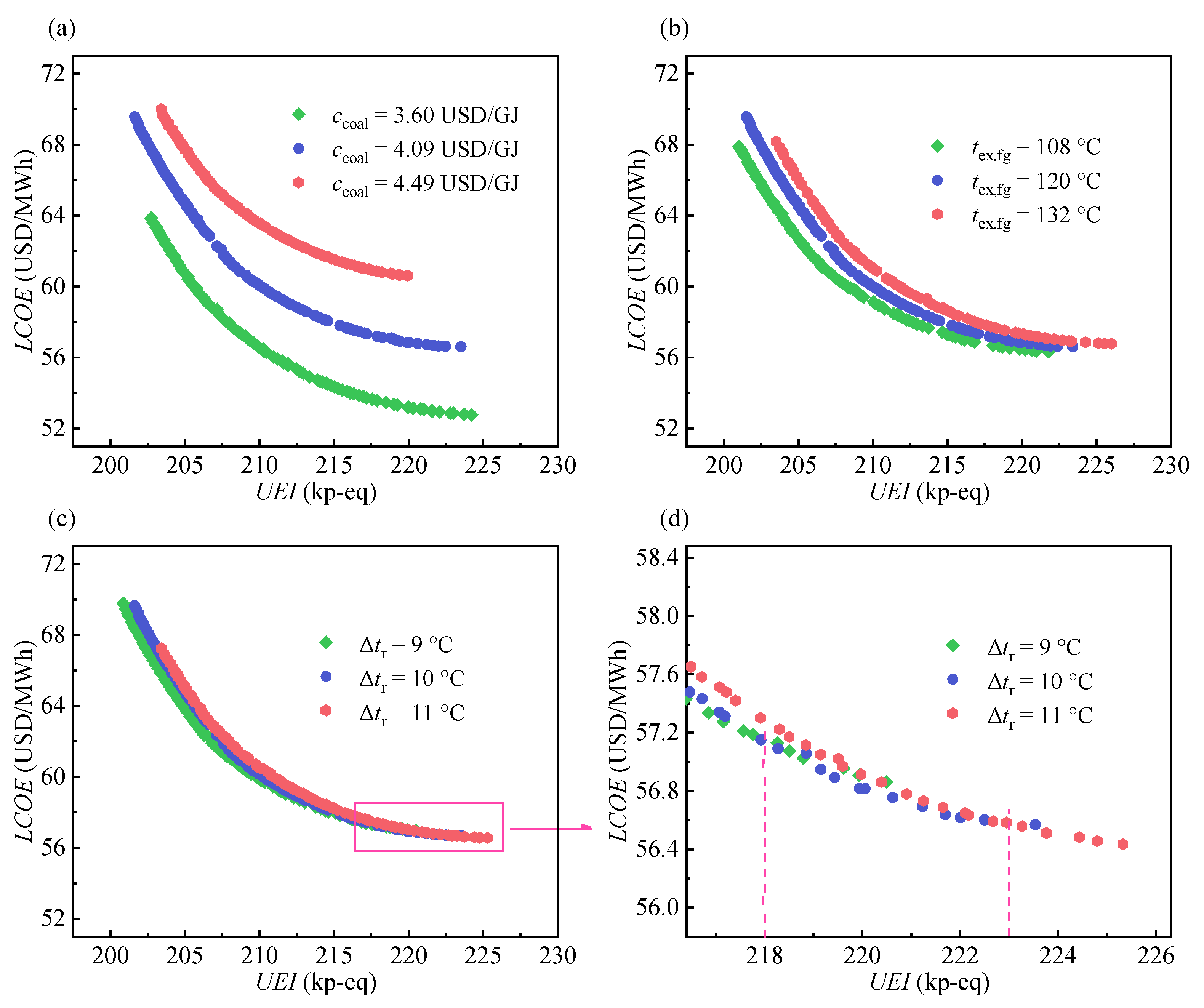
4.4. Sensitivity Analysis

A sensitivity analysis is conducted to explore the effect of the coal price per unit of heat (c_coal), exhaust temperature of flue gas (t_ex,fg), and the pinch temperature difference of the recuperator (Δt_r) on the Pareto frontier. Figure 17 displays the results with a ±10% variation in these three parameters. Figure 17d is the partial enlargement of Figure 17c. Based on observations and comparisons, the following three points are worth mentioning.

First, the c_coal shows the highest sensitivity, which is because the c_coal directly affects the FC_l. The t_ex,fg directly affects the boiler efficiency, further indirectly affecting the SC_l and FC_l. Hence, it has the second highest sensitivity. The Δt_r has the least relation with the SC_l and FC_l than others, and thus its sensitivity is the lowest.

Second, the distance between different the Pareto frontiers gradually increases with an increasing UEI in the case of the c_coal, which indicates that the sensitivity of c_coal to LCOE gradually increases with increasing UEI. This can be explained by the fact that in the high UEI region, the share of the FC_l to the total costs is larger than that in the low UEI region. Because c_coal is directly related to FC_l, high sensitivity appears in the high UEI region. In contrast, the sensitivities of t_ex,fg and Δt_r to LCOE gradually decrease with the increase in UEI.

Third, as shown in Figure 17d, the curves of the Pareto frontier intersect in the high UEI region in the case of Δt_r. When the UEI is below 218 kp-eq, the LCOE decreases with a decrease in the Δt_r for the same value of the UEI. In contrast, the LCOE increases when the UEI exceeds 223 kp-eq. For the former case, at the same UEI, the t_max and p_max will decrease with a decreasing Δt_r. Because the resultant cost reduction exceeds the increase in the recuperator cost, the LCOE is ultimately reduced. For the latter case, the resultant cost reduction is insufficient to offset the increasing recuperator cost, thus resulting in an increased LCOE.

5. Conclusions

In this study, environmental and economic objectives are considered to conduct layout comparison and parameter optimization of the SCO₂ coal-fired power generation system. Specifically, four typical and three improved layouts are compared to select the optimal layout. Subsequently, multi-objective optimization is performed to obtain the Pareto frontier of the selected layout. Further, for the Pareto frontier, characteristic and correlation analyses, decision process, and sensitivity analysis are successively conducted. The following conclusions are drawn.

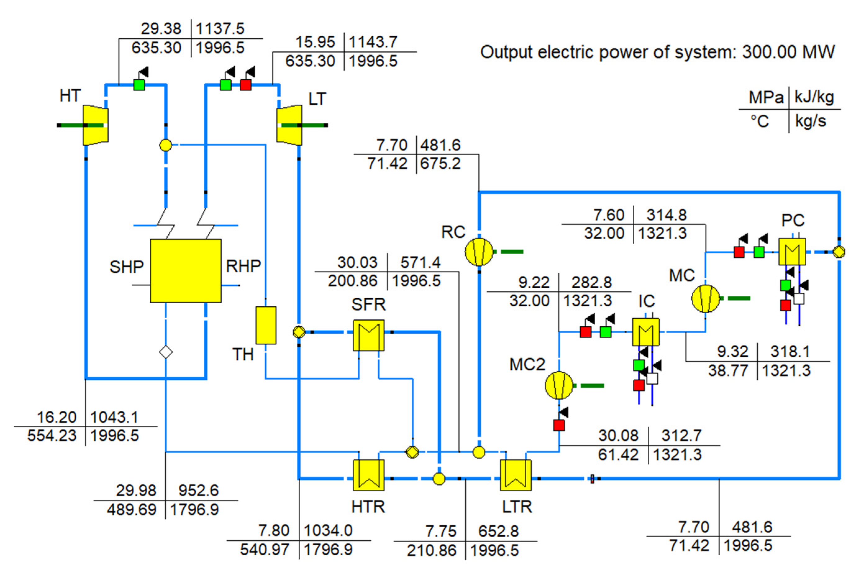
• Overlap is the optimal scheme for the extraction of tail flue gas energy, and intercooling is the optimal improved scheme. Case D3 is the optimal layout with the ultimate environmental impact (UEI) of 219.8 kp-eq and levelized cost of electricity (LCOE) of 56.9 USD/MWh.
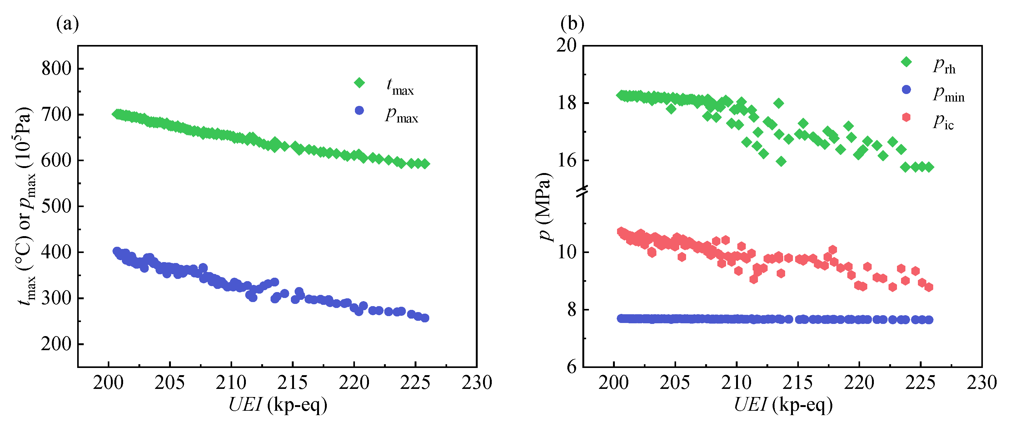
• The two objectives, namely, UEI and LCOE, conflict with each other. The Spearman correlation coefficient between the maximum temperature and pressure of the system is 0.966, which indicates that a coordination between them is required in the parameter design process.
• The decision optimal point shows a better comprehensive performance, the maximum temperature/pressure of which is 635.3 °C/30.1 MPa. Compared with economic and environmental optimal points, it takes 3.4% and 6.5% expenses in exchange for 5.3% and 17.7% benefits.
• The coal price per unit of heat shows the highest sensitivity and the sensitivity of it to the LCOE is higher in the higher UEI region. The pinch temperature difference of recuperator shows opposite sensitivities when the UEI is below 218 kp-eq and above 223 kp-eq.

At present, the concept of SCO₂ coal-fired power generation system is in the transition stage from theoretical study to engineering application. This study could provide some reference for the layout selection and parameter design of real systems in the future.

References

1. Li, P.; Hu, Q.Y.; Sun, Y.; Han, Z.H. Thermodynamic and economic performance analysis of heat and power cogeneration system based on advanced adiabatic compressed air energy storage coupled with solar auxiliary heat. J. Energy Storage 2021, 42, 103089. [Google Scholar] [CrossRef]
2. Li, P.; Hu, Q.Y.; Han, Z.H.; Wang, C.X.; Wang, R.X.; Han, X.; Wang, Y.Z. Thermodynamic analysis and multi-objective optimization of a trigenerative system based on compressed air energy storage under different working media and heating storage media. Energy 2022, 239, 122252. [Google Scholar] [CrossRef]
3. BP Statistical Review of World Energy. Available online: http://www.bp.com/statisticalreview (accessed on 30 June 2022).
4. Yang, Y.P.; Li, C.Z.; Wang, N.L.; Yang, Z.P. Progress and prospects of innovative coal-fired power plants within the energy internet. Glob. Energy Interconnect. 2019, 2, 160–179. [Google Scholar] [CrossRef]
5. Hofmann, M.; Tsatsaronis, G. Comparative exergoeconomic assessment of coal-fired power plants—Binary Rankine cycle versus conventional steam cycle. Energy 2018, 142, 168–179. [Google Scholar] [CrossRef]
6. Ahn, Y.; Bae, S.J.; Kim, M.; Cho, S.K.; Baik, S.; Lee, J.I.; Cha, J.E. Review of Supercritical CO2 Power Cycle Technology and Current Status of Research and Development. Nucl. Eng. Technol. 2015, 47, 647–661. [Google Scholar] [CrossRef]
7. Wang, X.; Wang, R.; Bian, X.; Cai, J.; Tian, H.; Shu, G.; Li, X.; Qin, Z. Review of dynamic performance and control strategy of supercritical CO2 Brayton cycle. Energy AI 2021, 5, 100078. [Google Scholar] [CrossRef]
8. Ehsan, M.M.; Guan, Z.Q.; Klimenko, A.Y. A comprehensive review on heat transfer and pressure drop characteristics and correlations with supercritical CO2 under heating and cooling applications. Renew. Sustain. Energy Rev. 2018, 92, 658–675. [Google Scholar] [CrossRef]
9. Liao, G.L.; Liu, L.J.; E, J.; Zhang, F.; Chen, J.W.; Deng, Y.W.; Zhu, H. Effects of technical progress on performance and application of supercritical carbon dioxide power cycle: A review. Energy Convers. Manag. 2019, 199, 111986. [Google Scholar] [CrossRef]
10. Xu, J.L.; Liu, C.; Sun, E.H.; Xie, J.; Li, M.J.; Yang, Y.P.; Liu, J.Z. Perspective of S-CO2 power cycles. Energy 2019, 186, 115831. [Google Scholar] [CrossRef]
11. Crespi, F.; Gavagnin, G.; Sanchez, D.; Martinez, G.S. Supercritical carbon dioxide cycles for power generation: A review. Appl. Energy 2017, 195, 152–183. [Google Scholar] [CrossRef]
12. White, M.T.; Bianchi, G.; Chai, L.; Tassou, S.A.; Sayma, A.I. Review of supercritical CO2 technologies and systems for power generation. Appl. Therm. Eng. 2021, 185, 116447. [Google Scholar] [CrossRef]
13. Yu, A.F.; Su, W.; Lin, X.X.; Zhou, N.J. Recent trends of supercritical CO2 Brayton cycle: Bibliometric analysis and research review. Nucl. Eng. Technol. 2021, 53, 699–714. [Google Scholar] [CrossRef]
14. Liu, M.; Zhang, X.W.; Ma, Y.G.; Yan, J.J. Thermo-economic analyses on a new conceptual system of waste heat recovery integrated with an S-CO2 cycle for coal-fired power plants. Energy Convers. Manag. 2018, 161, 243–253. [Google Scholar] [CrossRef]
15. Xu, C.; Zhang, Q.; Yang, Z.P.; Li, X.S.; Xu, G.; Yang, Y.P. An improved supercritical coal-fired power generation system incorporating a supplementary supercritical CO2 cycle. Appl. Energy 2018, 231, 1319–1329. [Google Scholar] [CrossRef]
16. Wang, D.; Xie, X.Y.; Wang, C.N.; Zhou, Y.L.; Yang, M.; Li, X.L.; Liu, D.Y. Thermo-economic analysis on an improved coal-fired power system integrated with S-CO2 brayton cycle. Energy 2021, 220, 119654. [Google Scholar] [CrossRef]
17. Hanak, D.P.; Manovic, V. Calcium looping with supercritical CO2 cycle for decarbonisation of coal-fired power plant. Energy 2016, 102, 343–353. [Google Scholar] [CrossRef]
18. Olumayegun, O.; Wang, M.H.; Oko, E. Thermodynamic performance evaluation of supercritical CO2 closed Brayton cycles for coal-fired power generation with solvent-based CO2 capture. Energy 2019, 166, 1074–1088. [Google Scholar] [CrossRef]
19. Wang, Y.J.; Xu, J.L.; Liu, Q.B.; Sun, E.H.; Chen, C. New combined supercritical carbon dioxide cycles for coal-fired power plants. Sustain. Cities Soc. 2019, 50, 101656. [Google Scholar] [CrossRef]
20. Zhou, J.; Zhu, M.; Tang, Y.F.; Xu, K.; Su, S.; Hu, S.; Wang, Y.; Xu, J.; He, L.M.; Xiang, J. Innovative system configuration analysis and design principle study for different capacity supercritical carbon dioxide coal-fired power plant. Appl. Therm. Eng. 2020, 174, 115298. [Google Scholar] [CrossRef]
21. Bai, W.G.; Li, H.Z.; Zhang, L.; Zhang, Y.F.; Yang, Y.; Zhang, C.; Yao, M.Y. Energy and exergy analyses of an improved recompression supercritical CO2 cycle for coal-fired power plant. Energy 2021, 222, 119976. [Google Scholar] [CrossRef]
22. Zhu, M.; Zhou, J.; Su, S.; Xu, J.; Li, A.S.; Chen, L.; Wang, Y.; Hu, S.; Jiang, L.; Xiang, J. Study on supercritical CO2 coal-fired boiler based on improved genetic algorithm. Energy Convers. Manag. 2020, 221, 113163. [Google Scholar] [CrossRef]
23. Wei, X.Y.; Manovic, V.; Hanak, D.P. Techno-economic assessment of coal- or biomass-fired oxy-combustion power plants with supercritical carbon dioxide cycle. Energy Convers. Manag. 2020, 221, 113143. [Google Scholar] [CrossRef]
24. Xu, J.L.; Wang, X.; Sun, E.H.; Li, M.J. Economic comparison between sCO2 power cycle and water-steam Rankine cycle for coal-fired power generation system. Energy Convers. Manag. 2021, 238, 114150. [Google Scholar] [CrossRef]
25. Sun, R.Q.; Yang, K.X.; Liu, M.; Yan, J.J. Thermodynamic and economic comparison of supercritical carbon dioxide coal-fired power system with different improvements. Int. J. Energy Res. 2021, 45, 9555–9579. [Google Scholar] [CrossRef]
26. Michalski, S.; Hanak, D.P.; Manovic, V. Advanced power cycles for coal-fired power plants based on calcium looping combustion: A techno-economic feasibility assessment. Appl. Energy 2020, 269, 114954. [Google Scholar] [CrossRef]
27. Thanganadar, D.; Asfand, F.; Patchigolla, K.; Turner, P. Techno-economic analysis of supercritical carbon dioxide cycle integrated with coal-fired power plant. Energy Convers. Manag. 2021, 242, 114294. [Google Scholar] [CrossRef]
28. Li, M.J.; Wang, G.; Xu, J.L.; Ni, J.W.; Sun, E.H. Life Cycle Assessment Analysis and Comparison of 1000 MW S-CO2 Coal Fired Power Plant and 1000 MW USC Water-Steam Coal-Fired Power Plant. J. Therm. Sci. 2020, 31, 463–484. [Google Scholar] [CrossRef]
29. Xu, J.L.; Sun, E.H.; Li, M.J.; Liu, H.; Zhu, B.G. Key issues and solution strategies for supercritical carbon dioxide coal fired power plant. Energy 2018, 157, 227–246. [Google Scholar] [CrossRef]
30. Zhou, J.; Zhang, C.H.; Su, S.; Wang, Y.; Hu, S.; Liu, L.; Ling, P.; Zhong, W.Q.; Xiang, J. Exergy analysis of a 1000 MW single reheat supercritical CO2 Brayton cycle coal-fired power plant. Energy Convers. Manag. 2018, 173, 348–358. [Google Scholar] [CrossRef]
31. Sun, E.H.; Xu, J.L.; Li, M.J.; Liu, G.L.; Zhu, B.G. Connected-top-bottom-cycle to cascade utilize flue gas heat for supercritical carbon dioxide coal fired power plant. Energy Convers. Manag. 2018, 172, 138–154. [Google Scholar] [CrossRef]
32. Sun, E.H.; Xu, J.L.; Hu, H.; Li, M.J.; Miao, Z.; Yang, Y.P.; Liu, J.Z. Overlap energy utilization reaches maximum efficiency for S-CO2 coal fired power plant: A new principle. Energy Convers. Manag. 2019, 195, 99–113. [Google Scholar] [CrossRef]
33. Moisseytsev, A.; Sienicki, J.J. Investigation of alternative layouts for the supercritical carbon dioxide Brayton cycle for a sodium-cooled fast reactor. Nucl. Eng. Des. 2009, 239, 1362–1371. [Google Scholar] [CrossRef]
34. STEAG Ebsilon Professional. Available online: http://www.ebsilon.com (accessed on 30 June 2022).
35. Thermophysical Properties of Fluid Systems. Available online: https://searchworks.stanford.edu/view/4136952 (accessed on 30 June 2022).
36. Zhang, Y.F.; Li, H.Z.; Han, W.L.; Bai, W.G.; Yang, Y.; Yao, M.Y.; Wang, Y.M. Improved design of supercritical CO2 Brayton cycle for coal-fired power plant. Energy 2018, 155, 1–14. [Google Scholar] [CrossRef]
37. Tong, Y.J.; Duan, L.Q.; Pang, L.P. Off-design performance analysis of a new 300 MW supercritical CO2 coal-fired boiler. Energy 2021, 216, 119306. [Google Scholar] [CrossRef]
38. Liu, M.; Yang, K.X.; Zhang, X.W.; Yan, J.J. Design and optimization of waste heat recovery system for supercritical carbon dioxide coal-fired power plant to enhance the dust collection efficiency. J. Cleaner Prod. 2020, 275, 122523. [Google Scholar] [CrossRef]
39. Zhou, J.; Ling, P.; Su, S.; Xu, J.; Xu, K.; Wang, Y.; Hu, S.; Zhu, M.; Xiang, J. Exergy analysis of a 1000 MW single reheat advanced supercritical carbon dioxide coal-fired partial flow power plant. Fuel 2019, 255, 115777. [Google Scholar] [CrossRef]
40. Bai, W.G.; Zhang, Y.F.; Yang, Y.; Li, H.Z.; Yao, M.Y. 300 MW boiler design study for coal-fired supercritical CO2 Brayton cycle. Appl. Therm. Eng. 2018, 135, 66–73. [Google Scholar] [CrossRef]
41. Bejan, A.; Tsatsaronis, G.; Moran, M. Thermal Design and Optimization; John Wiley & Sons: New York, NY, USA, 1996. [Google Scholar]
42. Weiland, N.T.; Lance, B.W.; Pidaparti, S.R. sCO2 Power Cycle Component Cost Correlations from DOE Data Spanning Multiple Scales and Applications. In Proceedings of the ASME Turbo Expo 2019: Turbomachinery Technical Conference and Exposition, Phoenix, AZ, USA, 17–21 June 2019. [Google Scholar]
43. Chen, D.X.; Han, Z.H.; Guo, D.Y.; Bai, Y.P.; Zhao, L.F. Exergoeconomic perspective to evaluate and optimize supercritical carbon dioxide coal-fired power generation system. Energy Convers. Manag. 2021, 244, 114482. [Google Scholar] [CrossRef]
44. Noaman, M.; Saade, G.; Morosuk, T.; Tsatsaronis, G. Exergoeconomic analysis applied to supercritical CO2 power systems. Energy 2019, 183, 756–765. [Google Scholar] [CrossRef]
45. Park, S.; Kim, J.; Yoon, M.; Rhim, D.; Yeom, C. Thermodynamic and economic investigation of coal-fired power plant combined with various supercritical CO2 Brayton power cycle. Appl. Therm. Eng. 2018, 130, 611–623. [Google Scholar] [CrossRef]
46. Mecheri, M. SCO2 closed Brayton cycle for coal-fired power plant: An economic analysis of a technical optimization. In Proceedings of the 2nd European sCO2 Conference, Essen, Germany, 30–31 August 2018; pp. 127–134. [Google Scholar]
47. Xu, C.; Li, X.S.; Xin, T.T.; Liu, X.; Xu, G.; Wang, M.; Yang, Y.P. A thermodynamic analysis and economic assessment of a modified de-carbonization coal-fired power plant incorporating a supercritical CO2 power cycle and an absorption heat transformer. Energy 2019, 179, 30–45. [Google Scholar] [CrossRef]
48. Handbook on Life Cycle Assessment. Available online: https://www.universiteitleiden.nl/en/research/research-projects/science/cml-new-dutch-lca-guide (accessed on 30 June 2022).
49. Yang, J.X.; Xu, C.; Wang, R.S. Product Life Cycle Evaluation Method and Application; China Meteorological Press: Beijing, China, 2002. (In Chinese) [Google Scholar]
50. Rasheed, R.; Javed, H.; Rizwan, A.; Sharif, F.; Yasar, A.; Tabinda, A.B.; Ahmad, S.R.; Wang, Y.B.; Su, Y.H. Life cycle assessment of a cleaner supercritical coal-fired power plant. J. Cleaner Prod. 2021, 279, 123869. [Google Scholar] [CrossRef]
51. Han, Y.; Sun, Y.Y. Collaborative optimization of energy conversion and NOx removal in boiler cold-end of coal-fired power plants based on waste heat recovery of flue gas and sensible heat utilization of extraction steam. Energy 2020, 207, 118172. [Google Scholar] [CrossRef]
52. Skorek-Osikowska, A.; Bartela, L.; Kotowicz, J. Thermodynamic and ecological assessment of selected coal-fired power plants integrated with carbon dioxide capture. Appl. Energy 2017, 200, 73–88. [Google Scholar] [CrossRef]
53. CML-IA Characterisation Factors. Available online: https://www.universiteitleiden.nl/en/research/research-output/science/cml-ia-characterisation-factors (accessed on 30 June 2022).
54. Deb, K.; Pratap, A.; Agarwal, S.; Meyarivan, T. A fast and elitist multiobjective genetic algorithm: NSGA-II. IEEE Trans. Evol. Comput. 2002, 6, 182–197. [Google Scholar] [CrossRef]
55. Mathworks MATLAB. Available online: https://www.mathworks.com (accessed on 30 June 2022).
56. Liu, Z.J.; Guo, J.C.; Wu, D.; Fan, G.Y.; Zhang, S.C.; Yang, X.Y.; Ge, H. Two-phase collaborative optimization and operation strategy for a new distributed energy system that combines multi-energy storage for a nearly zero energy community. Energy Convers. Manag. 2021, 230, 113800. [Google Scholar] [CrossRef]
57. Hwang, C.-L.; Yoon, K. (Eds.) Methods for Multiple Attribute Decision Making. In Multiple Attribute Decision Making; Springer: Berlin/Heidelberg, Germany, 1981; pp. 58–191. [Google Scholar] [CrossRef]
58. Rao, Z.H.; Xue, T.C.; Huang, K.X.; Liao, S.M. Multi-objective optimization of supercritical carbon dioxide recompression Brayton cycle considering printed circuit recuperator design. Energy Convers. Manag. 2019, 201, 112094. [Google Scholar] [CrossRef]
59. Forthofer, R.N.; Lee, E.S.; Hernandez, M. (Eds.) 3—Descriptive Methods. In Biostatistics, 2nd ed.; Academic Press: San Diego, CA, USA, 2007; pp. 21–69. [Google Scholar] [CrossRef]
Figure 1. The basic layout coupled with four extraction schemes of tail flue gas energy: (Case A) LTR parallel scheme. (Case B) HTR parallel scheme. (Case C) Top-bottom scheme. (Case D) Overlap scheme.
Entropy 24 01123 g001
Figure 3. The logic flowchart of Section 3.
Entropy 24 01123 g003
Figure 4. The flowchart of the gamultiobj algorithm.
Entropy 24 01123 g004
Figure 5. The diagram of the second and third steps of the TOPSIS method.
Entropy 24 01123 g005
Figure 6. Comparison of four typical layouts: (a) UEI and LCOE. (b) levelized system costs (SCl) and levelized fuel costs (FCl).
Entropy 24 01123 g006
Figure 7. Comparison of three improved layouts: (a) UEI and LCOE. (b) levelized system costs (SCl) and levelized fuel costs (FCl).
Entropy 24 01123 g007
Figure 8. The Pareto frontier of different generations: (a) 100th generation. (b) 200th generation. (c) 400th generation. (d) 800th generation.
Entropy 24 01123 g008
Figure 9. The variation of design parameters: (a) tmax and pmax. (b) prh, pmin, and pic.
Entropy 24 01123 g009
Figure 10. The variation of system output parameters: (a) input heat rate of boiler, total power output of turbines, and the total power consumption of compressors. (b) total recuperation rate and mass flow rate of SCO2.
Entropy 24 01123 g010
Figure 11. The variation of levelized costs.
Entropy 24 01123 g011
Figure 12. The variation of PEC: (a) PEC over 20 M/USD. (b) PEC below 20 M/USD.
Entropy 24 01123 g012
Figure 13. The relation between two parameters: (a) prh and tmax. (b) prh and pmax.
Entropy 24 01123 g013
Figure 14. Three optimal points in the Pareto frontier.
Entropy 24 01123 g014
Figure 15. The ingredient distribution: (a) UEI. (b) LCOE.
Entropy 24 01123 g015
Figure 16. The Ebsilon model of the system with Case D3 layout and DOP parameters.
Entropy 24 01123 g016
Figure 17. Sensitivity analysis for different parameters: (a) coal price per unit of heat. (b) exhaust temperature of flue gas. (c,d) pinch temperature difference of recuperator.
Entropy 24 01123 g017