
Semi-Quantitative MALDI Measurements of Blood-Based Samples for Molecular Diagnostics

 ,
,
Abstract
:
1. Introduction
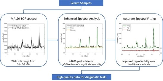
2. Results
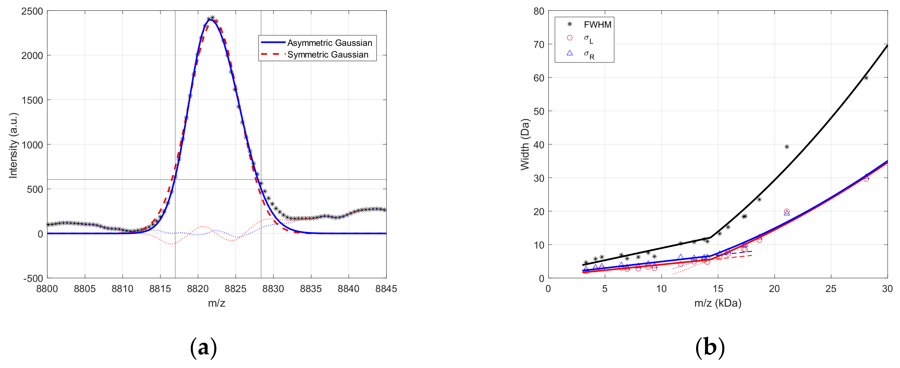
2.1. MALDI Peak Shape Analysis
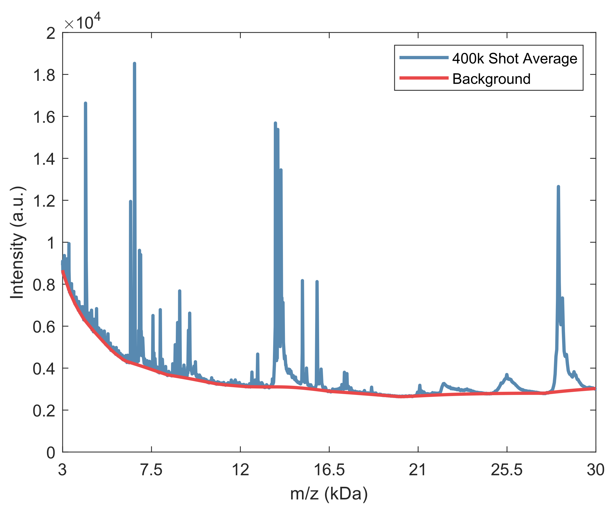
2.2. Spectral Analysis of Deep MALDI Spectra
2.2.1. Background Estimation
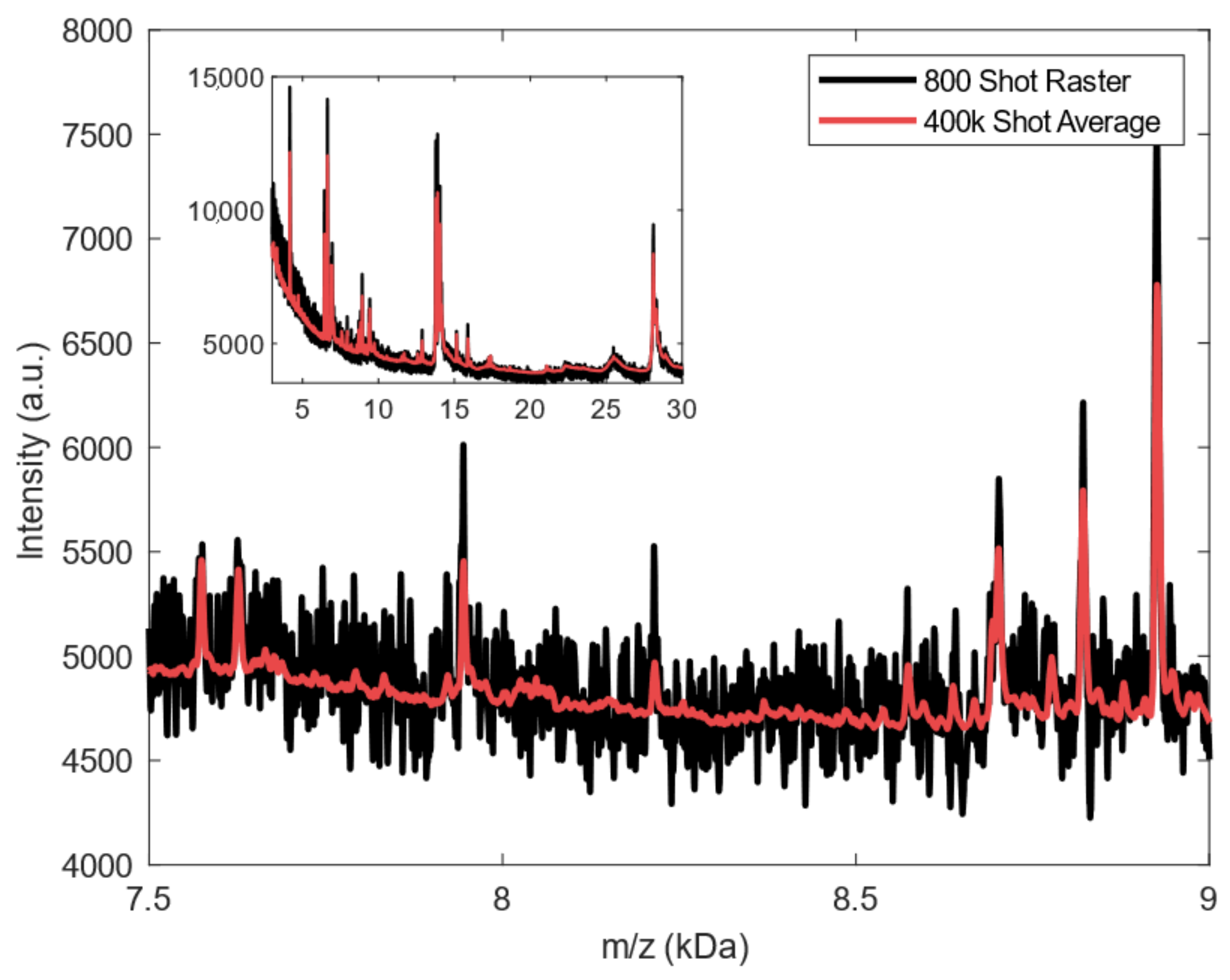
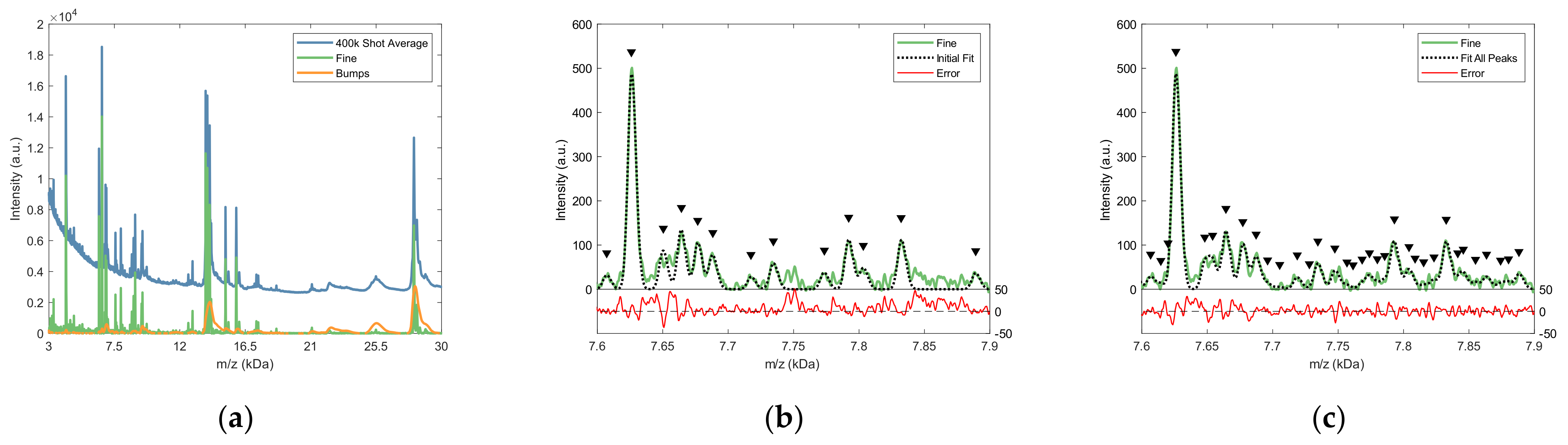
2.2.2. Fine Structure Determination and Peak Fitting
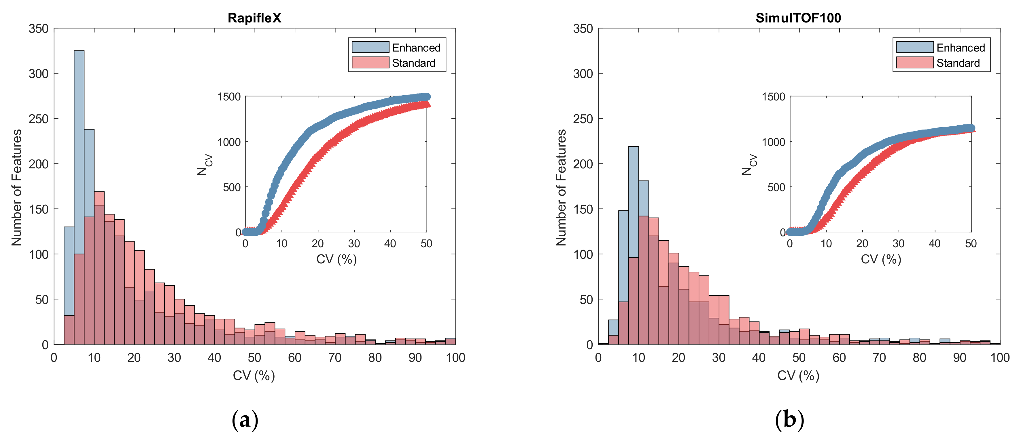
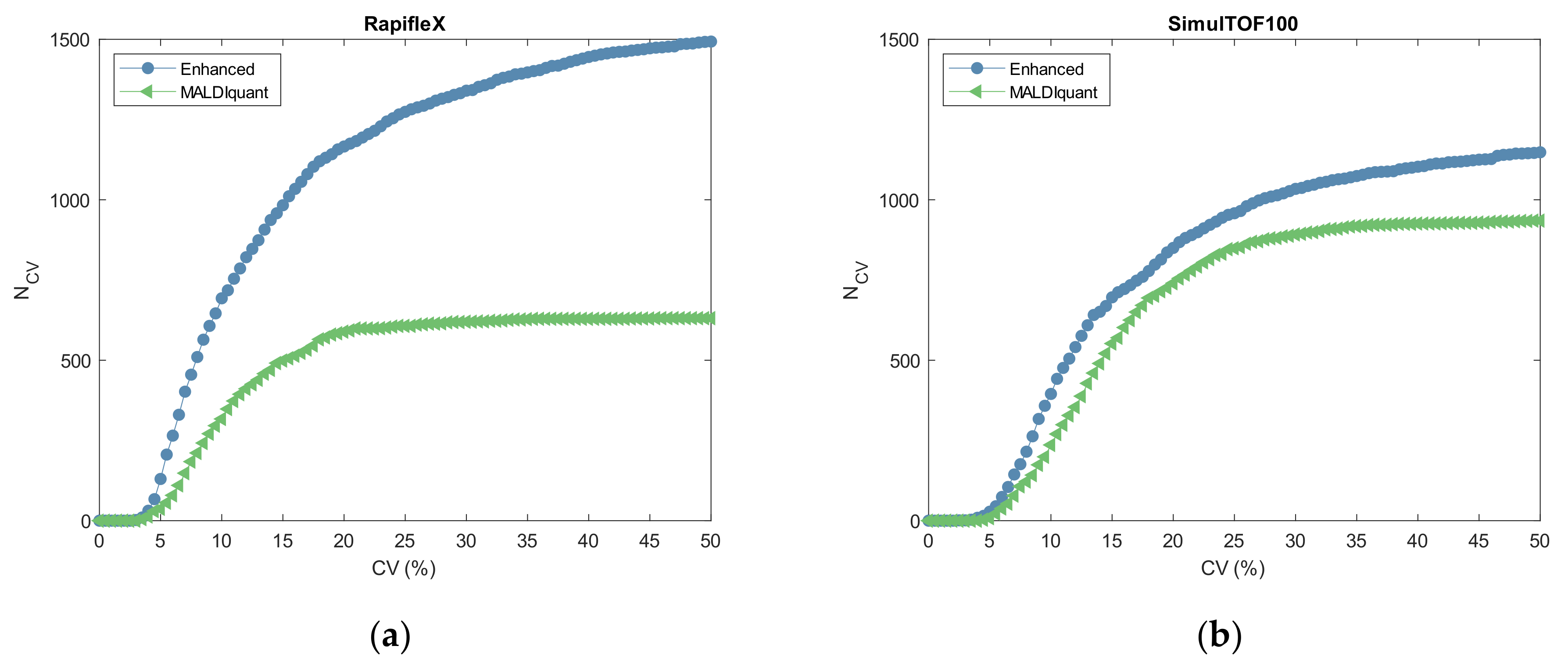
2.3. Reproducibility
2.4. Association with Biological Processes
3. Discussion
3.1. MALDI Peak Shape Analysis
3.2. Peak Detection and Feature Value Determination
3.3. Reproducibility
3.4. PSEA
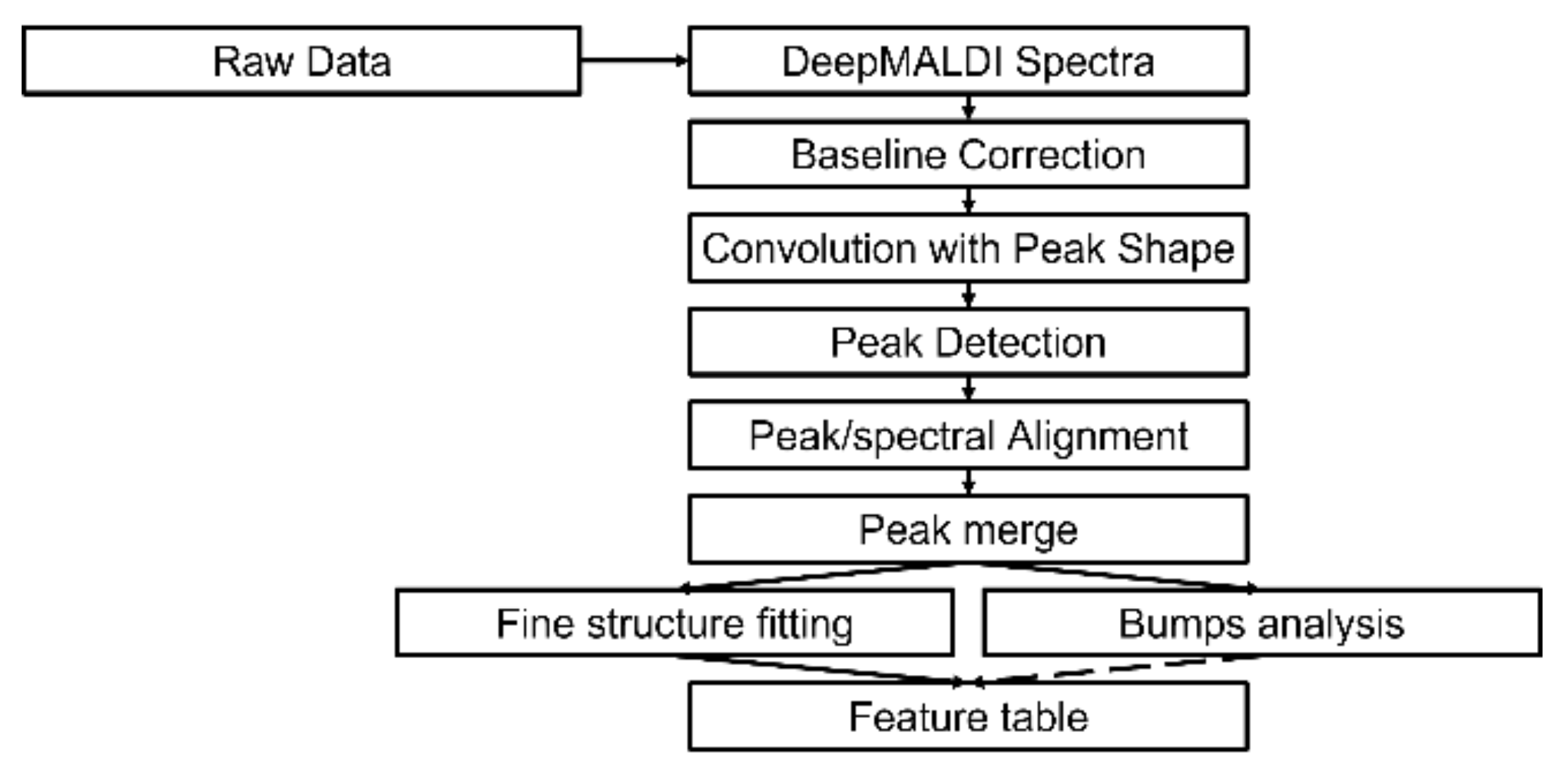
4. Materials and Methods
4.1. Serum Samples
4.2. Sample Preparation
4.3. Mass Spectra Acquisition
4.3.1. RapifleX
4.3.2. SimulTOF100
4.4. Spectral Analysis
4.4.1. Raster Averaging for Deep MALDI Spectra
4.4.2. Background Estimation
4.4.3. Fine Structure and Bumps Determination
4.4.4. Peak Detection
4.4.5. Spectral Alignment
4.4.6. Feature Value Determination
4.4.7. MALDIquant Analysis
4.5. Peak Shape Fitting
4.6. Merge Peak Lists
4.7. Reproducibility Analysis
4.8. Association with Biological Processes
5. Conclusions
Supplementary Materials
Author Contributions
Funding
Institutional Review Board Statement
Informed Consent Statement
Data Availability Statement
Acknowledgments
Conflicts of Interest
Sample Availability
References
- Bast, R., Jr.; Xu, F.-J.; Yu, Y.-H.; Barnhill, S.; Zhang, Z.; Mills, G. CA 125: The Past and the Future. Int. J. Biol. Markers 1998, 13, 179–187. [Google Scholar] [CrossRef] [PubMed]
- Scarà, S.; Bottoni, P.; Scatena, R. CA 19-9: Biochemical and Clinical Aspects. Adv. Cancer Biomark. 2015, 867, 247–260. [Google Scholar] [CrossRef]
- Dorcely, B.; Katz, K.; Jagannathan, R.; Chiang, S.S.; Oluwadare, B.; Goldberg, I.J.; Bergman, M. Novel Biomarkers for Prediabetes, Diabetes, and Associated Complications. Diabetes Metab. Syndr. Obes. Targets Ther. 2017, 10, 345. [Google Scholar] [CrossRef] [PubMed] [Green Version]
- Patel, S.P.; Kurzrock, R. PD-L1 Expression as a Predictive Biomarker in Cancer Immunotherapy. Mol. Cancer Ther. 2015, 14, 847–856. [Google Scholar] [CrossRef] [PubMed] [Green Version]
- Johnson, P.J.; Pirrie, S.J.; Cox, T.F.; Berhane, S.; Teng, M.; Palmer, D.; Morse, J.; Hull, D.; Patman, G.; Kagebayashi, C.; et al. The Detection of Hepatocellular Carcinoma Using a Prospectively Developed and Validated Model Based on Serological Biomarkers. Cancer Epidemiol. Prev. Biomark. 2014, 23, 144–153. [Google Scholar] [CrossRef] [PubMed] [Green Version]
- Tsypin, M.; Asmellash, S.; Meyer, K.; Touchet, B.; Roder, H. Extending the Information Content of the MALDI Analysis of Biological Fluids via Multi-Million Shot Analysis. PLoS ONE 2019, 14, e0226012. [Google Scholar] [CrossRef] [Green Version]
- Roder, J.; Oliveira, C.; Net, L.; Tsypin, M.; Linstid, B.; Roder, H. A Dropout-Regularized Classifier Development Approach Optimized for Precision Medicine Test Discovery from Omics Data. BMC Bioinform. 2019, 20, 325. [Google Scholar] [CrossRef] [Green Version]
- Roder, H.; Oliveira, C.; Net, L.; Linstid, B.; Tsypin, M.; Roder, J. Robust Identification of Molecular Phenotypes Using Semi-Supervised Learning. BMC Bioinform. 2019, 20, 273. [Google Scholar] [CrossRef] [Green Version]
- Taguchi, F.; Solomon, B.; Gregorc, V.; Roder, H.; Gray, R.; Kasahara, K.; Nishio, M.; Brahmer, J.; Spreafico, A.; Ludovini, V.; et al. Mass Spectrometry to Classify Non–Small-Cell Lung Cancer Patients for Clinical Outcome after Treatment with Epidermal Growth Factor Receptor Tyrosine Kinase Inhibitors: A Multicohort Cross-Institutional Study. J. Natl. Cancer Inst. 2007, 99, 838–846. [Google Scholar] [CrossRef] [Green Version]
- Weber, J.S.; Sznol, M.; Sullivan, R.J.; Blackmon, S.; Boland, G.; Kluger, H.M.; Halaban, R.; Bacchiocchi, A.; Ascierto, P.A.; Capone, M.; et al. A Serum Protein Signature Associated with Outcome after Anti–PD-1 Therapy in Metastatic Melanoma. Cancer Immunol. Res. 2018, 6, 79–86. [Google Scholar] [CrossRef] [Green Version]
- Mahalingam, D.; Chelis, L.; Nizamuddin, I.; Lee, S.S.; Kakolyris, S.; Halff, G.; Washburn, K.; Attwood, K.; Fahad, I.; Grigorieva, J.; et al. Detection of Hepatocellular Carcinoma in a High-Risk Population by a Mass Spectrometry-Based Test. Cancers 2021, 13, 3109. [Google Scholar] [CrossRef] [PubMed]
- Grigorieva, J.; Asmellash, S.; Net, L.; Tsypin, M.; Roder, H.; Roder, J. Mass Spectrometry-Based Multivariate Proteomic Tests for Prediction of Outcomes on Immune Checkpoint Blockade Therapy: The Modern Analytical Approach. Int. J. Mol. Sci. 2020, 21, 838. [Google Scholar] [CrossRef] [PubMed] [Green Version]
- Kasimir-Bauer, S.; Roder, J.; Obermayr, E.; Mahner, S.; Vergote, I.; Loverix, L.; Braicu, E.; Sehouli, J.; Concin, N.; Kimmig, R.; et al. Definition and Independent Validation of a Proteomic-Classifier in Ovarian Cancer. Cancers 2020, 12, 2519. [Google Scholar] [CrossRef] [PubMed]
- Ascierto, P.A.; Capone, M.; Grimaldi, A.M.; Mallardo, D.; Simeone, E.; Madonna, G.; Roder, H.; Meyer, K.; Asmellash, S.; Oliveira, C.; et al. Proteomic Test for Anti-PD-1 Checkpoint Blockade Treatment of Metastatic Melanoma with and without BRAF Mutations. J. Immunother. Cancer 2019, 7, 91. [Google Scholar] [CrossRef] [PubMed]
- Carbone, D.P.; Salmon, J.S.; Billheimer, D.; Chen, H.; Sandler, A.; Roder, H.; Roder, J.; Tsypin, M.; Herbst, R.S.; Tsao, A.S.; et al. VeriStrat® Classifier for Survival and Time to Progression in Non-Small Cell Lung Cancer (NSCLC) Patients Treated with Erlotinib and Bevacizumab. Lung Cancer 2010, 69, 337–340. [Google Scholar] [CrossRef] [Green Version]
- Carbone, D.P.; Ding, K.; Roder, H.; Grigorieva, J.; Roder, J.; Tsao, M.-S.; Seymour, L.; Shepherd, F.A. Prognostic and Predictive Role of the VeriStrat Plasma Test in Patients with Advanced Non–Small-Cell Lung Cancer Treated with Erlotinib or Placebo in the NCIC Clinical Trials Group BR. 21 Trial. J. Thorac. Oncol. 2012, 7, 1653–1660. [Google Scholar] [CrossRef] [Green Version]
- Kuiper, J.; Lind, J.; Groen, H.; Roder, J.; Grigorieva, J.; Roder, H.; Dingemans, A.; Smit, E. VeriStrat® Has Prognostic Value in Advanced Stage NSCLC Patients Treated with Erlotinib and Sorafenib. Br. J. Cancer 2012, 107, 1820–1825. [Google Scholar] [CrossRef] [PubMed] [Green Version]
- Gautschi, O.; Dingemans, A.-M.; Crowe, S.; Peters, S.; Roder, H.; Grigorieva, J.; Roder, J.; Zappa, F.; Pless, M.; Brutsche, M.; et al. VeriStrat® Has a Prognostic Value for Patients with Advanced Non-Small Cell Lung Cancer Treated with Erlotinib and Bevacizumab in the First Line: Pooled Analysis of SAKK19/05 and NTR528. Lung Cancer 2013, 79, 59–64. [Google Scholar] [CrossRef]
- Stinchcombe, T.E.; Roder, J.; Peterman, A.H.; Grigorieva, J.; Lee, C.B.; Moore, D.T.; Socinski, M.A. A Retrospective Analysis of VeriStrat Status on Outcome of a Randomized Phase II Trial of First-Line Therapy with Gemcitabine, Erlotinib, or the Combination in Elderly Patients (Age 70 Years or Older) with Stage IIIB/IV Non–Small-Cell Lung Cancer. J. Thorac. Oncol. 2013, 8, 443–451. [Google Scholar] [CrossRef] [Green Version]
- Grossi, F.; Genova, C.; Rijavec, E.; Barletta, G.; Biello, F.; Dal Bello, M.G.; Meyer, K.; Roder, J.; Roder, H.; Grigorieva, J. Prognostic Role of the VeriStrat Test in First Line Patients with Non-Small Cell Lung Cancer Treated with Platinum-Based Chemotherapy. Lung Cancer 2018, 117, 64–69. [Google Scholar] [CrossRef] [Green Version]
- Fidler, M.J.; Fhied, C.L.; Roder, J.; Basu, S.; Sayidine, S.; Fughhi, I.; Pool, M.; Batus, M.; Bonomi, P.; Borgia, J.A. The Serum-Based VeriStrat® Test Is Associated with Proinflammatory Reactants and Clinical Outcome in Non-Small Cell Lung Cancer Patients. BMC Cancer 2018, 18, 310. [Google Scholar] [CrossRef] [PubMed]
- Yasui, Y.; McLerran, D.; Adam, B.-L.; Winget, M.; Thornquist, M.; Feng, Z. An Automated Peak Identification/Calibration Procedure for High-Dimensional Protein Measures from Mass Spectrometers. J. Biomed. Biotechnol. 2003, 2003, 242. [Google Scholar] [CrossRef] [PubMed] [Green Version]
- Morris, J.S.; Coombes, K.R.; Koomen, J.; Baggerly, K.A.; Kobayashi, R. Feature Extraction and Quantification for Mass Spectrometry in Biomedical Applications Using the Mean Spectrum. Bioinformatics 2005, 21, 1764–1775. [Google Scholar] [CrossRef] [PubMed] [Green Version]
- Gibb, S.; Strimmer, K. MALDIquant: A Versatile R Package for the Analysis of Mass Spectrometry Data. Bioinformatics 2012, 28, 2270–2271. [Google Scholar] [CrossRef] [PubMed]
- Lange, E.; Gröpl, C.; Reinert, K.; Kohlbacher, O.; Hildebrandt, A. High-Accuracy Peak Picking of Proteomics Data Using Wavelet Techniques. In Biocomputing 2006; World Scientific: Singapore, 2006; pp. 243–254. [Google Scholar]
- Du, P.; Kibbe, W.A.; Lin, S.M. Improved Peak Detection in Mass Spectrum by Incorporating Continuous Wavelet Transform-Based Pattern Matching. Bioinformatics 2006, 22, 2059–2065. [Google Scholar] [CrossRef] [PubMed] [Green Version]
- Dubrovkin, J. Evaluation of the Peak Location Uncertainty in Second-Order Derivative Spectra. Case Study: Symmetrical Lines. Int. J. Emerg. Technol. Comput. Appl. Sci. 2014, 7, 45–53. [Google Scholar]
- Picaud, V.; Giovannelli, J.-F.; Truntzer, C.; Charrier, J.-P.; Giremus, A.; Grangeat, P.; Mercier, C. Linear MALDI-ToF Simultaneous Spectrum Deconvolution and Baseline Removal. BMC Bioinform. 2018, 19, 123. [Google Scholar] [CrossRef] [Green Version]
- Grigorieva, J.; Asmellash, S.; Oliveira, C.; Roder, H.; Net, L.; Roder, J. Application of Protein Set Enrichment Analysis to Correlation of Protein Functional Sets with Mass Spectral Features and Multivariate Proteomic Tests. Clin. Mass Spectrom. 2020, 15, 44–53. [Google Scholar] [CrossRef]
- Trede, D.; Kobarg, J.H.; Oetjen, J.; Thiele, H.; Maass, P.; Alexandrov, T. On the Importance of Mathematical Methods for Analysis of MALDI-Imaging Mass Spectrometry Data. J. Integr. Bioinforma. JIB 2012, 9, 189. [Google Scholar] [CrossRef]
- Eilers, P.H.; Boelens, H.F. Baseline Correction with Asymmetric Least Squares Smoothing. Leiden Univ. Med. Cent. Rep. 2005, 1, 5. [Google Scholar]
- Boelens, H.F.; Dijkstra, R.J.; Eilers, P.H.; Fitzpatrick, F.; Westerhuis, J.A. New Background Correction Method for Liquid Chromatography with Diode Array Detection, Infrared Spectroscopic Detection and Raman Spectroscopic Detection. J. Chromatogr. A 2004, 1057, 21–30. [Google Scholar] [CrossRef] [PubMed]
- Senko, M.W.; Beu, S.C.; McLaffertycor, F.W. Determination of Monoisotopic Masses and Ion Populations for Large Biomolecules from Resolved Isotopic Distributions. J. Am. Soc. Mass Spectrom. 1995, 6, 229–233. [Google Scholar] [CrossRef] [Green Version]
- Blaum, K.; Geppert, C.; Müller, P.; Nörtershäuser, W.; Wendt, K.; Bushaw, B. Peak Shape for a Quadrupole Mass Spectrometer: Comparison of Computer Simulation and Experiment. Int. J. Mass Spectrom. 2000, 202, 81–89. [Google Scholar] [CrossRef]
- Foxon, C.; Joyce, B.; Holloway, S. Instrument Response Function of a Quadrupole Mass Spectrometer Used in Time-of-Flight Measurements. Int. J. Mass Spectrom. Ion Phys. 1976, 21, 241–255. [Google Scholar] [CrossRef]
- Osborn, D.L.; Zou, P.; Johnsen, H.; Hayden, C.C.; Taatjes, C.A.; Knyazev, V.D.; North, S.W.; Peterka, D.S.; Ahmed, M.; Leone, S.R. The Multiplexed Chemical Kinetic Photoionization Mass Spectrometer: A New Approach to Isomer-Resolved Chemical Kinetics. Rev. Sci. Instrum. 2008, 79, 104103. [Google Scholar] [CrossRef] [Green Version]
- Yang, C.; He, Z.; Yu, W. Comparison of Public Peak Detection Algorithms for MALDI Mass Spectrometry Data Analysis. BMC Bioinform. 2009, 10, 4. [Google Scholar] [CrossRef] [Green Version]
- Danielsson, R.; Bylund, D.; Markides, K.E. Matched Filtering with Background Suppression for Improved Quality of Base Peak Chromatograms and Mass Spectra in Liquid Chromatography–Mass Spectrometry. Anal. Chim. Acta 2002, 454, 167–184. [Google Scholar] [CrossRef]
- Ahn, S.-M.; Simpson, R.J. Body Fluid Proteomics: Prospects for Biomarker Discovery. PROTEOMICS–Clin. Appl. 2007, 1, 1004–1015. [Google Scholar] [CrossRef]
- Müller, A.C.; Breitwieser, F.P.; Fischer, H.; Schuster, C.; Brandt, O.; Colinge, J.; Superti-Furga, G.; Stingl, G.; Elbe-Bürger, A.; Bennett, K.L. A Comparative Proteomic Study of Human Skin Suction Blister Fluid from Healthy Individuals Using Immunodepletion and ITRAQ Labeling. J. Proteome Res. 2012, 11, 3715–3727. [Google Scholar] [CrossRef]
- Subramanian, A.; Tamayo, P.; Mootha, V.K.; Mukherjee, S.; Ebert, B.L.; Gillette, M.A.; Paulovich, A.; Pomeroy, S.L.; Golub, T.R.; Lander, E.S.; et al. Gene Set Enrichment Analysis: A Knowledge-Based Approach for Interpreting Genome-Wide Expression Profiles. Proc. Natl. Acad. Sci. USA 2005, 102, 15545–15550. [Google Scholar] [CrossRef] [Green Version]
- Roder, J.; Linstid, B.; Oliveira, C. Improving the Power of Gene Set Enrichment Analyses. BMC Bioinform. 2019, 20, 257. [Google Scholar] [CrossRef] [PubMed] [Green Version]
- Savitzky, A.; Golay, M.J.E. Smoothing and Differentiation of Data by Simplified Least Squares Procedures. Anal. Chem. 1964, 36, 1627–1639. [Google Scholar] [CrossRef]
- Ryan, C.G.; Clayton, E.; Griffin, W.L.; Sie, S.H.; Cousens, D.R. SNIP, a Statistics-Sensitive Background Treatment for the Quantitative Analysis of PIXE Spectra in Geoscience Applications. Nucl. Instrum. Methods Phys. Res. Sect. B Beam Interact. Mater. At. 1988, 34, 396–402. [Google Scholar] [CrossRef]
- Tibshirani, R.; Hastie, T.; Narasimhan, B.; Soltys, S.; Shi, G.; Koong, A.; Le, Q.-T. Sample Classification from Protein Mass Spectrometry, by “Peak Probability Contrasts. Bioinformatics 2004, 20, 3034–3044. [Google Scholar] [CrossRef] [PubMed] [Green Version]
- Gold, L.; Ayers, D.; Bertino, J.; Bock, C.; Bock, A.; Brody, E.; Carter, J.; Cunningham, V.; Dalby, A.; Eaton, B.; et al. Aptamer-Based Multiplexed Proteomic Technology for Biomarker Discovery. PLoS ONE 2010, 5, e16004. [Google Scholar] [CrossRef] [Green Version]
- Kraemer, S.; Vaught, J.D.; Bock, C.; Gold, L.; Katilius, E.; Keeney, T.R.; Kim, N.; Saccomano, N.A.; Wilcox, S.K.; Zichi, D.; et al. From SOMAmer-Based Biomarker Discovery to Diagnostic and Clinical Applications: A SOMAmer-Based, Streamlined Multiplex Proteomic Assay. PLoS ONE 2011, 6, e26332. [Google Scholar] [CrossRef] [PubMed] [Green Version]
- Benjamini, Y.; Hochberg, Y. Controlling the False Discovery Rate: A Practical and Powerful Approach to Multiple Testing. J. R. Stat. Soc. Ser. B Methodol. 1995, 57, 289–300. [Google Scholar] [CrossRef]


| FWHM | 2.878 | 5.89 × 10⁻⁴ | 5.764 | −1.13 × 10⁻³ | 1.05 × 10⁻⁷ | 14,471 |
| 1.374 | 2.55 × 10⁻⁴ | −3.143 | −9.53 × 10⁻⁶ | 3.99 × 10⁻⁸ | ||
| 1.504 | 3.33 × 10⁻⁴ | 8.907 | −1.12 × 10⁻³ | 6.54 × 10⁻⁸ |
| Biological Process | Associated Features | ||
|---|---|---|---|
| RapifleX | SimulTOF | Ref. [6] | |
| Acute phase response | 655 (43.2%) | 460 (40.6%) | 122 (40.9%) |
| Complement activation | 619 (40.8%) | 383 (33.7%) | 70 (23.5%) |
| Acute inflammatory response | 434 (28.6%) | 317 (27.9%) | 109 (36.6%) |
| IFN γ signaling/response | 266 (17.5%) | 147 (12.9%) | 25 (8.4%) |
| Immune tolerance and suppression | 227 (15.0%) | 189 (16.6%) | 31 (10.4%) |
| Wound healing | 202 (13.3%) | 160 (14.1%) | 100 (33.6%) |
| IFN type 1 signaling/response | 195 (12.9%) | 82 (7.2%) | 33 (11.1%) |
| Type 17 immune response | 73 (4.8%) | 82 (7.2%) | 2 (0.7%) |
| Angiogenesis | 54 (3.6%) | 28 (2.5%) | 2 (0.7%) |
| Response to hypoxia | 42 (2.8%) | 54 (4.7%) | 7 (2.3%) |
| Cellular component morphogenesis | 27 (1.8%) | 6 (0.5%) | 4 (1.3%) |
| Cytokine production involved in immune response | 21 (1.4%) | 31 (2.7%) | 3 (1.0%) |
| Glycolysis | 21 (1.4%) | 36 (3.2%) | 2 (0.7%) |
| Chronic inflammatory response | 19 (1.3%) | 23 (2.0%) | 2 (0.7%) |
| Innate immune response | 18 (1.2%) | 30 (2.6%) | 8 (2.7%) |
| Extracellular matrix organization | 16 (1.1%) | 4 (0.4%) | 0 (0.0%) |
| Behavior | 7 (0.5%) | 2 (0.2%) | 8 (2.7%) |
| Epithelial-mesenchymal transition | 6 (0.4%) | 4 (0.4%) | 0 (0.0%) |
| NK cell mediated immunity | 4 (0.3%) | 11 (1.0%) | N/A * |
| T-cell mediated immunity | 4 (0.3%) | 5 (0.4%) | N/A * |
| Type 2 immune response | 2 (0.1%) | 11 (1.0%) | N/A * |
| B-cell mediated immunity | 2 (0.1%) | 6 (0.5%) | N/A * |
| Type 1 immune response | 1 (0.1%) | 1 (0.1%) | N/A * |
Publisher’s Note: MDPI stays neutral with regard to jurisdictional claims in published maps and institutional affiliations. |
© 2022 by the authors. Licensee MDPI, Basel, Switzerland. This article is an open access article distributed under the terms and conditions of the Creative Commons Attribution (CC BY) license (https://creativecommons.org/licenses/by/4.0/).
Share and Cite
Koc, M.A.; Asmellash, S.; Norman, P.; Rightmyer, S.; Roder, J.; Georgantas, R.W., III; Roder, H. Semi-Quantitative MALDI Measurements of Blood-Based Samples for Molecular Diagnostics. Molecules 2022, 27, 997. https://0-doi-org.brum.beds.ac.uk/10.3390/molecules27030997
Koc MA, Asmellash S, Norman P, Rightmyer S, Roder J, Georgantas RW III, Roder H. Semi-Quantitative MALDI Measurements of Blood-Based Samples for Molecular Diagnostics. Molecules. 2022; 27(3):997. https://0-doi-org.brum.beds.ac.uk/10.3390/molecules27030997
Chicago/Turabian StyleKoc, Matthew A., Senait Asmellash, Patrick Norman, Steven Rightmyer, Joanna Roder, Robert W. Georgantas, III, and Heinrich Roder. 2022. "Semi-Quantitative MALDI Measurements of Blood-Based Samples for Molecular Diagnostics" Molecules 27, no. 3: 997. https://0-doi-org.brum.beds.ac.uk/10.3390/molecules27030997