Article

Western Pacific Zooplankton Community along Latitudinal and Equatorial Transects in Autumn 2017 (Northern Hemisphere)

1
Research Centre for Indian Ocean Ecosystem, Tianjin University of Science and Technology, Tianjin 300457, China
2
College of Marine Science and Technology, China University of Geosciences (Wuhan), Wuhan 430074, China
3
Institute of Marine Science and Technology, Shandong University, Qingdao 266200, China
4
Key Laboratory of Marine Chemistry Theory and Technology, Ministry of Education, Ocean University of China, Qingdao 266100, China
5
College of Marine Life Science, Ocean University of China, Qingdao 266003, China
*
Author to whom correspondence should be addressed.
Submission received: 2 November 2020 / Revised: 28 January 2021 / Accepted: 28 January 2021 / Published: 3 February 2021
(This article belongs to the Special Issue Linking Plankton Diversity with Ecosystem Functioning and Services)

Abstract

:
During the autumn of 2017, a study was conducted to assess the zooplankton community composition in three sections (two latitudinal, going from Japan to the equator, and one longitudinal on the equator) of the Western Pacific Ocean. A total of 384 species of zooplankton adults and 21 groups of zooplankton larvae were identified, with copepods being the predominant taxon. The common dominant species across the three sections were Acrocalanus gibber, Canthocalanus pauper, Oithona similis, Paracalanus aculeatus, and Oncaea venusta. Zooplankton abundance was the highest in the equator section, with a mean abundance of 258.94 ± 52.57 ind./m3. Comparatively, a low abundance was recovered from the Subtropical Countercurrent (STCC) region, while the highest abundance holding stations were located in the eastern equatorial and North Equatorial Countercurrent (NECC) regions. Pearson’s correlation, canonical correspondence analysis, and other methods were used to analyze the relationship between environmental factors and zooplankton. We found that the Shannon–Wiener diversity index and Pielou’s uniformity index were significantly correlated (p < 0.05) with concentrations of nitrite and chlorophyll a. The distribution of zooplankton was also limited by nutrients, chlorophyll a, and dissolved oxygen. In addition, we reveal differences in the abundance of species in the equatorial and latitudinal seas. We found that not only temperature and nutrient salinity, but also ocean currents and the movement of water masses, influence the distribution of zooplankton communities in the Western Pacific.

1. Introduction

The presence of many atolls, island groups, and seamounts in the Western Pacific Ocean [1,2] has altered the trajectory of ocean circulation, resulting in a variety of complex vertical hydrographic features and current patterns [3], including in the major oceanic circulations such as the Kuroshio Current System and the Equatorial Current System. In addition, the equatorial Western Pacific Ocean possesses the largest warm water mass in the global ocean, the Western Pacific Warm Pool (WPWP). The WPWP, with an annual mean surface seawater temperature of not less than 28 °C, has a profound impact on global climate change, especially in China and Southeast Asia, by heating seawater, transferring radiant heat to the atmosphere, and using latent heat to transport evaporative heat [4]. The Western Pacific is of great interest due to its unique geography, ocean circulation, and special climatic characteristics [5]. Its unique environment nurtures unique ecological habitats, and the complex currents also make the region a biodiversity hotspot [6,7] and a source of global marine life [8,9], containing a high level of biodiversity [10,11].
As an intermediate part of the marine food chain [12], zooplankton play an important role in marine ecosystems [13] and in marine biogeochemical cycles [14]. Moreover, the zooplankton can be used for surveillance of large economic fish communities in the pelagic marine ecosystem [15,16]. Due to the complex geography of the Western Pacific and the importance of zooplankton, there is a growing interest in the study of zooplankton in the open waters of the Western Pacific Ocean. For example, in recent years, Dai et al. [17] conducted a zooplankton survey of Philippine waters in winter based on the Zooscan instrument and found that zooplankton abundance distribution was highest in the North Equatorial Countercurrent zone (NECC) and lowest in the Northern Equatorial Current zone (NEC). Similarly, a fall study by Yang et al. [18] in the same area yielded similar results, with the highest zooplankton abundance distribution in the NECC zone and then the NEC zone, and the lowest in the Subtropical Countercurrent zone (STCC). The abundance of zooplankton communities generally increases with latitude in summer studies along 160° E, as found by Sun et al. [19]. However, the latitudinal span between these studies is large and does not provide a good fit to the overall zooplankton distribution in the region. Also, compared to studies in the Central and Eastern Pacific [20,21,22], there is relatively little information on zooplankton in the Western Equatorial Pacific.
This study was carried out in the Western Pacific along 143° E, east of Japan at 146° E and the equator, focusing on the zooplankton community composition and the factors regulating it. The aim of the present work was to reveal the community composition of zooplankton in the equatorial Western Pacific and to enrich zooplankton research in the Western Pacific.

2. Materials and Methods

From 6 October to 7 December 2017, we conducted a trawl survey of zooplankton from 0 to 200 m in the Western Pacific using the WP2 net (200-µm mesh, 0.2 m2 mouth size) aboard the scientific vessel Dongfanghong 2. A calibrated flowmeter (Hydrobios) was equipped on the WP2 net to measure the volume of filtered seawater. As shown in Figure 1, the survey area was divided into three sections: Section 1 (S1, located at the east of the Japan along 146° E), Section 2 (S2, assigned to the longitude of 143° E) and Section 3 (S3, assigned along the equator). A total of 59 net samples were eventually collected.
The net samples were collected in 500-mL polyethylene (PE) bottles, fixed with 5% formaldehyde solution (final concentration), and kept in the dark until they were brought back to the laboratory for further analysis. Prior to microscopic analysis, large zooplankton, such as jellyfish of the spinifex phylum, were picked out and counted in their entirety. For microscopic analysis, at least 1% of the total volume of the remaining sample (depending on the sample density) was placed in the DSJ plankton counting frame. Zooplankton abundances (ind./m3) for each station were calculated using the total volume of filtered water, expressed as ind./m3. A total of 59 subsamples were examined under the microscope (Motic Panthrea L and Motic SMZ-168 SERIES) at 40–100× magnification to identify them to the lowest possible taxonomic level. Temperature and salinity were measured during the voyage using a Seabird CTD 911. The temperature and salinity of the water column were calculated by means of a trapezoidal integration of the different levels of seawater temperature and salinity. The pH of the water sample was determined using a pH meter. Dissolved oxygen (DO) was determined immediately by the Winkler method after the CTD arrived on deck. Nitrate, nitrite, ammonium, phosphate, and silicate were also analyzed on board by spectrometric methods [23]. The dissolved inorganic carbon [21] concentration was measured using a Shimadzu TOC-L analyzer equipped with an ASI-V auto-sampler, using the total inorganic carbon mode.
As a measure of the diversity of the zooplankton community, we analyzed the dominance index, the Shannon–Wiener diversity index, Pielou’s evenness index, Simpson’s diversity index, and Margalef’s diversity index (Y, H′, J, D, and Dm, respectively) as follows [24]:
Y = n i N f i
H = i = 1 S P i log 2 P i
J = H log 2 S
D = i = 1 S P i 2   ,   P i 2 = n i ( n i ) N ( N 1 )
D m a = ( S 1 ) ln N
where S represents the zooplankton species in each sample, also known as species richness; N represents the total number of cells in all samples, ni represents the number of cells of the ith species, Pi represents the cell abundance of the ith species, Pi = ni/Ni, and fi represents the frequency of occurrence of the ith species in a single sample.
Ocean Data View 4.10 was used for figures depicting the horizontal distribution of zooplankton. The relationship between zooplankton and environmental parameters was analyzed by the canonical correspondence analysis (CCA; Canoco 4.5). The multidimensional scaling (MDS) was constructed using Primer 6.0. The Pearson correlation was analyzed using Statistical Product and Service Solutions (SPSS).

3. Results

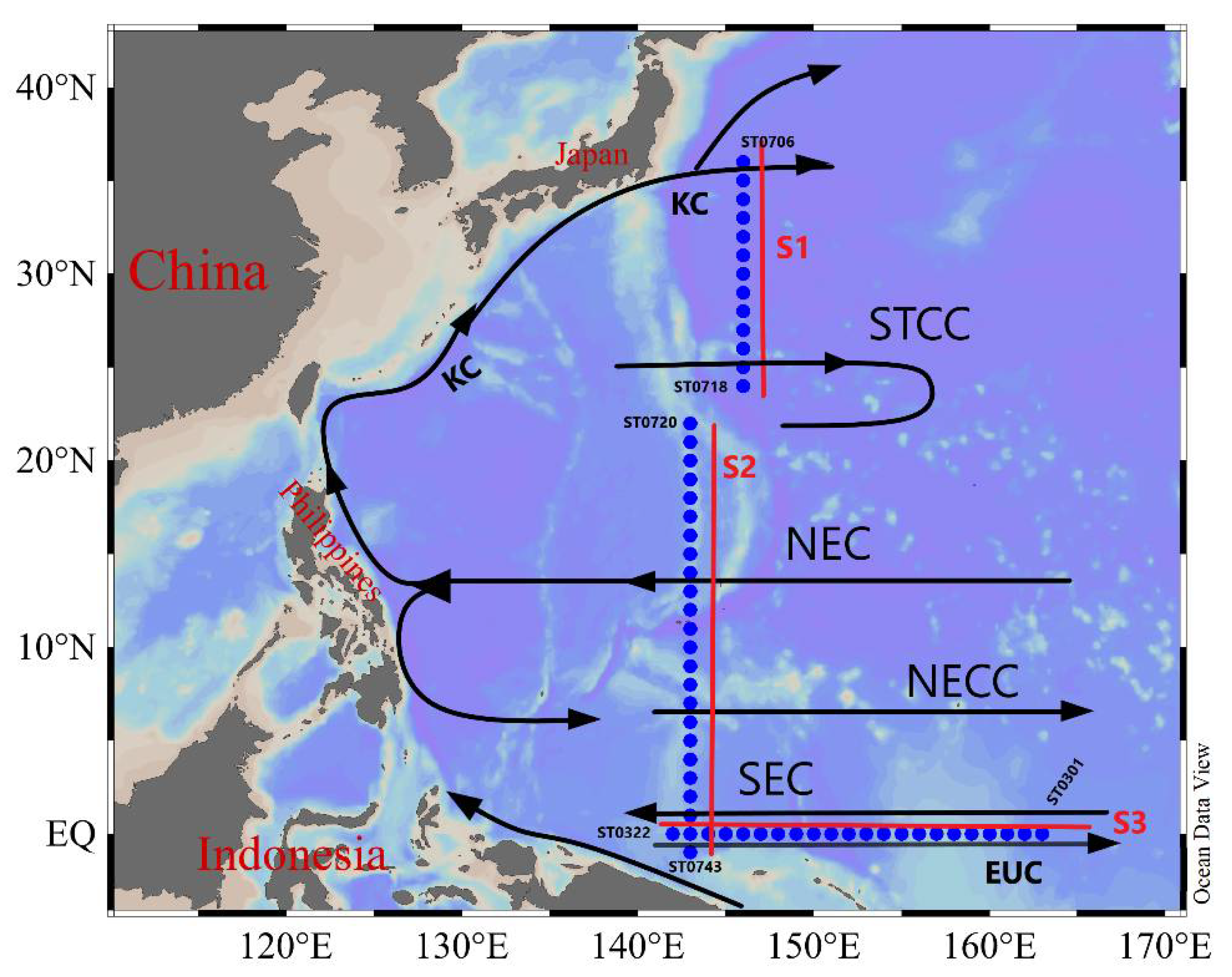
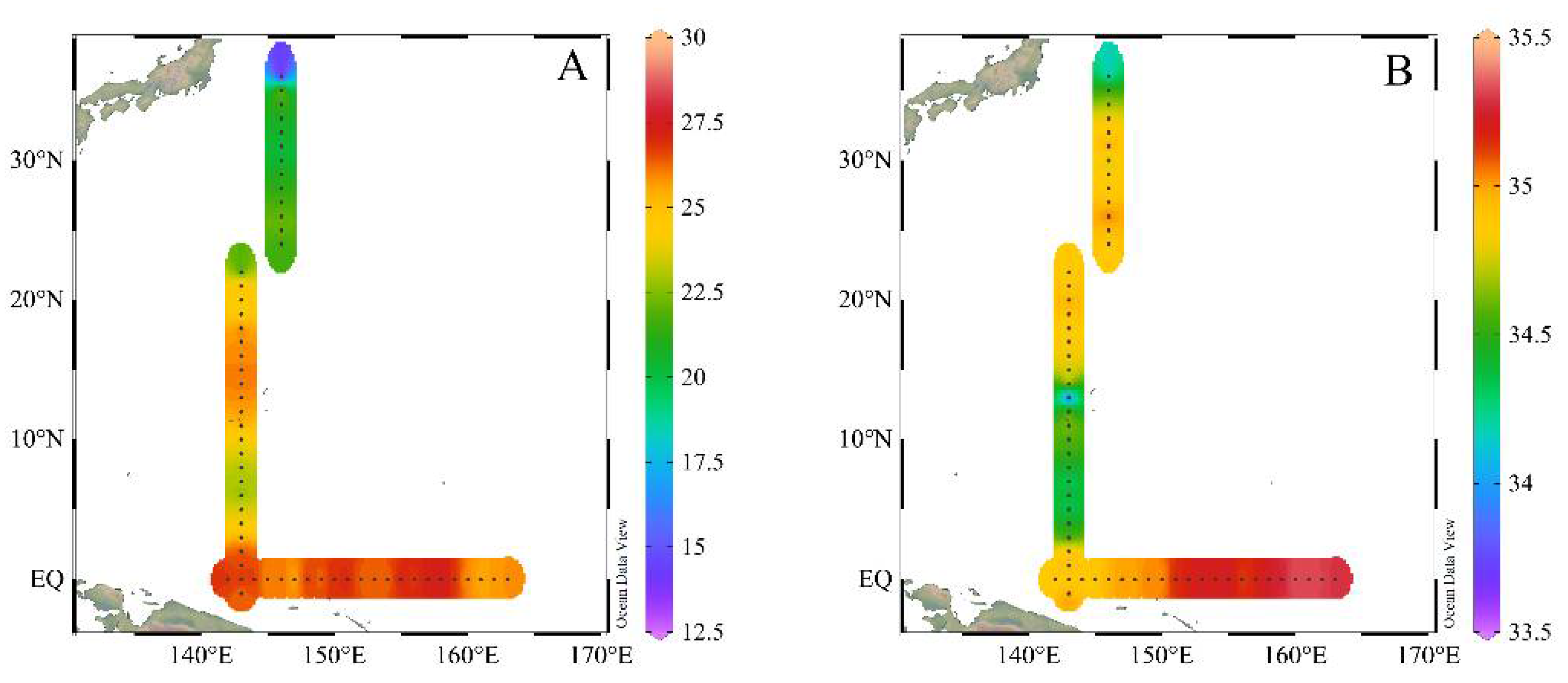
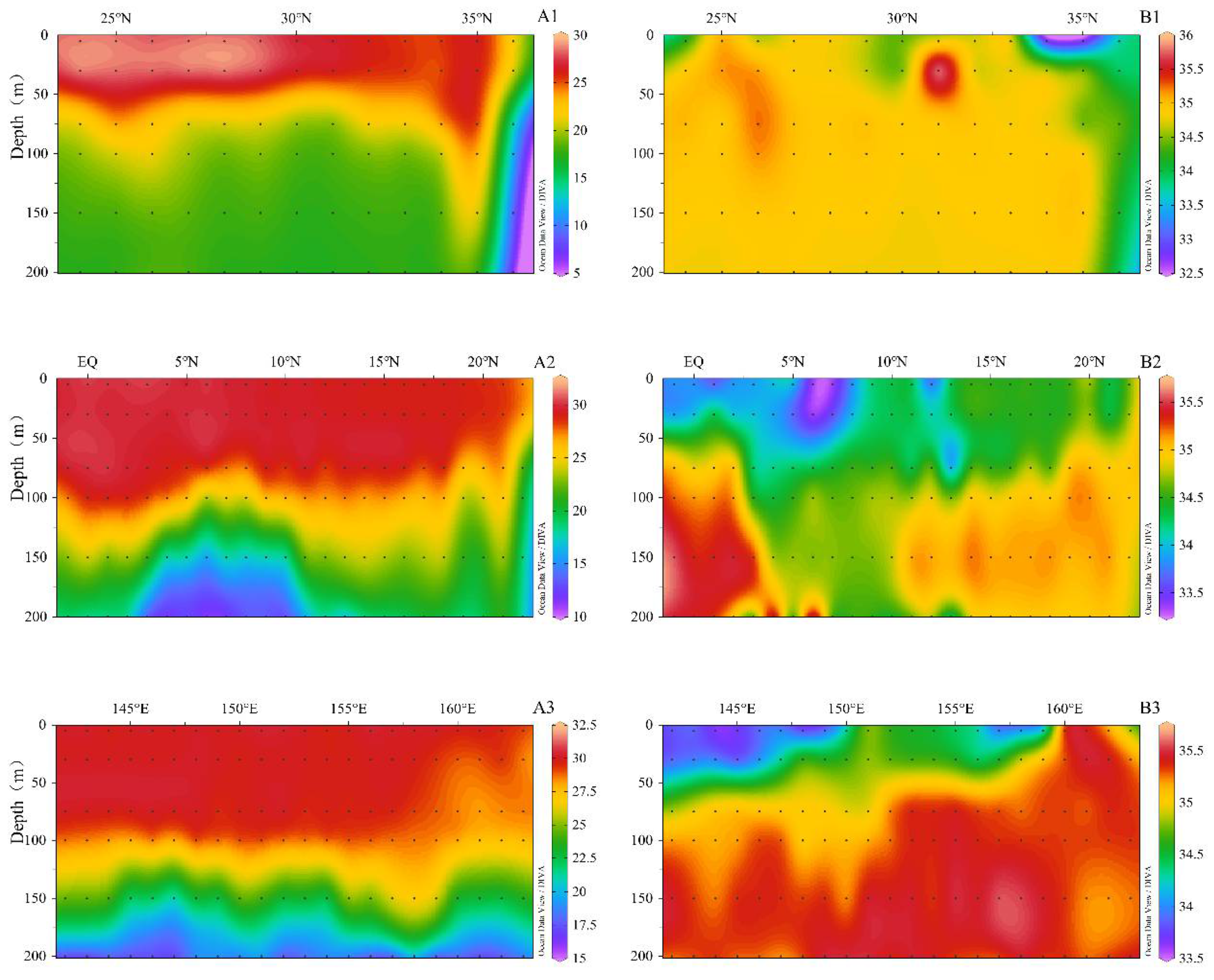
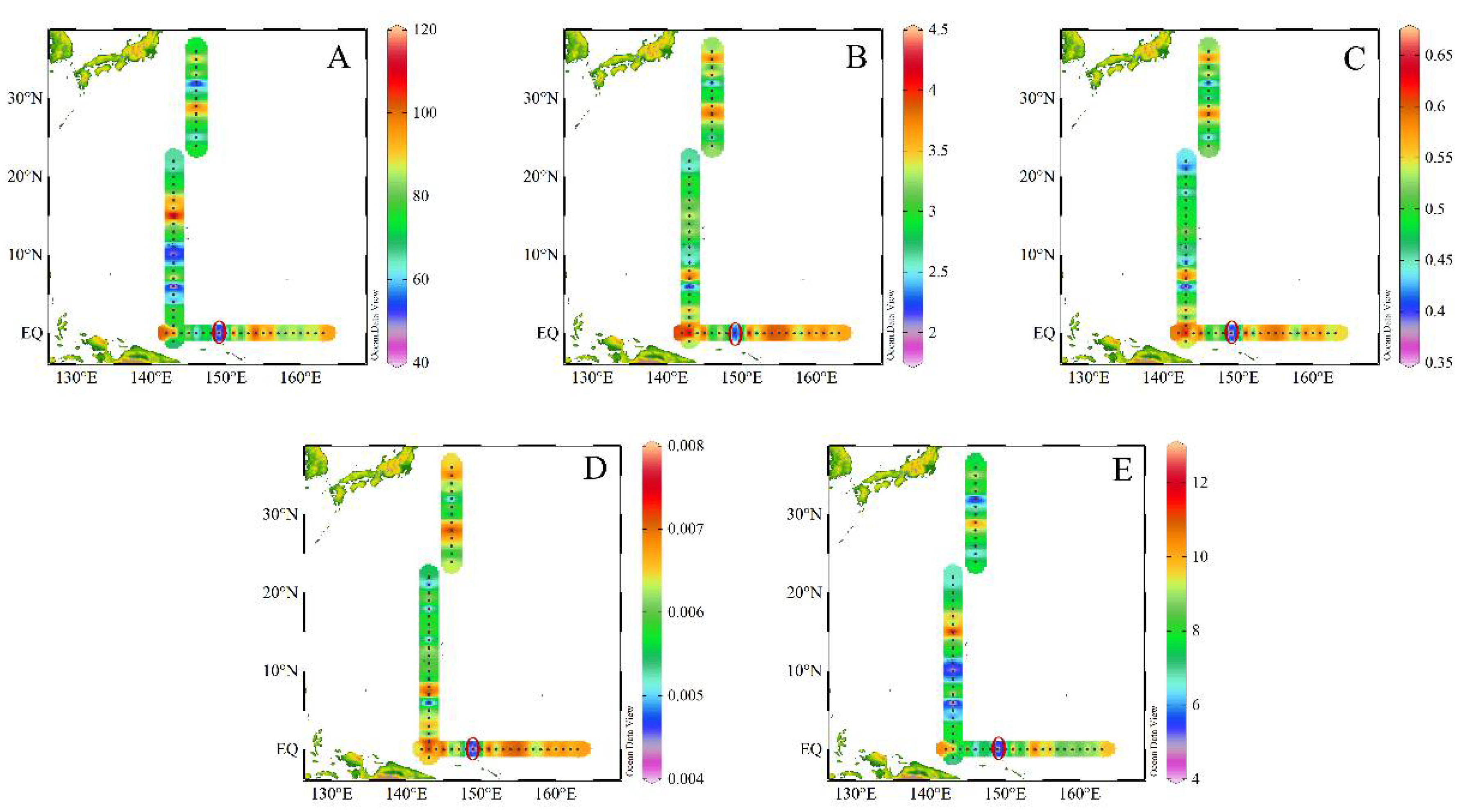
3.1. Hydrography of the Study Area

The ocean circulation pattern in the study area is drawn according to the previous literature [25,26] and represented in Figure 1. The water column was integrated with the temperature and salinity at the upper 200 m layer in the survey area, and the results are shown in Figure 2. Under the influence of the warm pool in the Western Pacific Ocean, the temperature of the seawater at the equator is mostly greater than 27.5 °C [27], and the temperature of the seawater decreases with the increase in latitude. In contrast, the waters with little variation in salinity and relatively low salinity were at 5–12° N and west of the equatorial section. The whole study area was divided into three main transects (Figure 3). Section 1 (S1) is mainly located east of Japan (146° E). There is an obvious trend of decreasing seawater temperature at the surface of this section with increasing latitude. This section is affected by the Oyashio Undercurrent and the Kuroshio Current, which resulted in a significant temperature and salinity change at ST0706 and ST0707. The temperature and salinity in this area were lower than at the other stations (Figure 3).
Section 2 (S2) was assigned to the longitude of 143° E, which mainly passes through the ocean circulation, including the North Equatorial Current, the North Equatorial Countercurrent, and the South Equatorial Current (Figure 1). It can be seen from the S2 cross-sectional temperature and salinity profiles that there was an upward current between 3° and 10° N. This also explains why the temperature and salinity of the sea area around 5–10° N in horizontal distribution (Figure 2) are lower than those of the surrounding stations (Figure 3).
The S3 section was assigned along the equator and was mainly influenced by the equatorial undertow and the southern equatorial current. The seawater temperature was above 27 °C from the surface to 75 m (Figure 3). With increasing depth, the temperature gradually decreases from about 30 °C at the surface to about 15 °C in the 200 m water layer, and vertical stratification was found below 100 m. Above the 50-m layer, the salinity was low in the west and high in the east, and spreads eastward along the depth, probably due to the influence of high-temperature low-salinity water in the Western Pacific warm pool [28] and the upwelling of high-salinity water in the subsurface layer by the south equatorial current in the east [29].

3.2. Zooplankton Species Composition

A total of 384 species of zooplankton and 21 groups of zooplankton larvae were identified in this survey. The zooplankton adults included 28 species of Protozoa, 18 species of Coelenterata, 6 species of Annelida, 16 species of Mollusca, 265 species of Arthropoda, 21 species of Chaetognatha, and 31 species of Chordata. Among the zooplankton adults, copepods contributed 217 species, accounting for 56.51% of the total number of species in the surveyed area and 81.89% of the total number of arthropod species. On average, 78 ± 16 number of species were identified per station, with the highest number of species (118) at station ST0727. Copepods had the highest numbers of species in the equatorial section with 56 + 12, followed by the S1 section with 52 + 13; the lowest number of species was in the S3 section with 48 + 11.

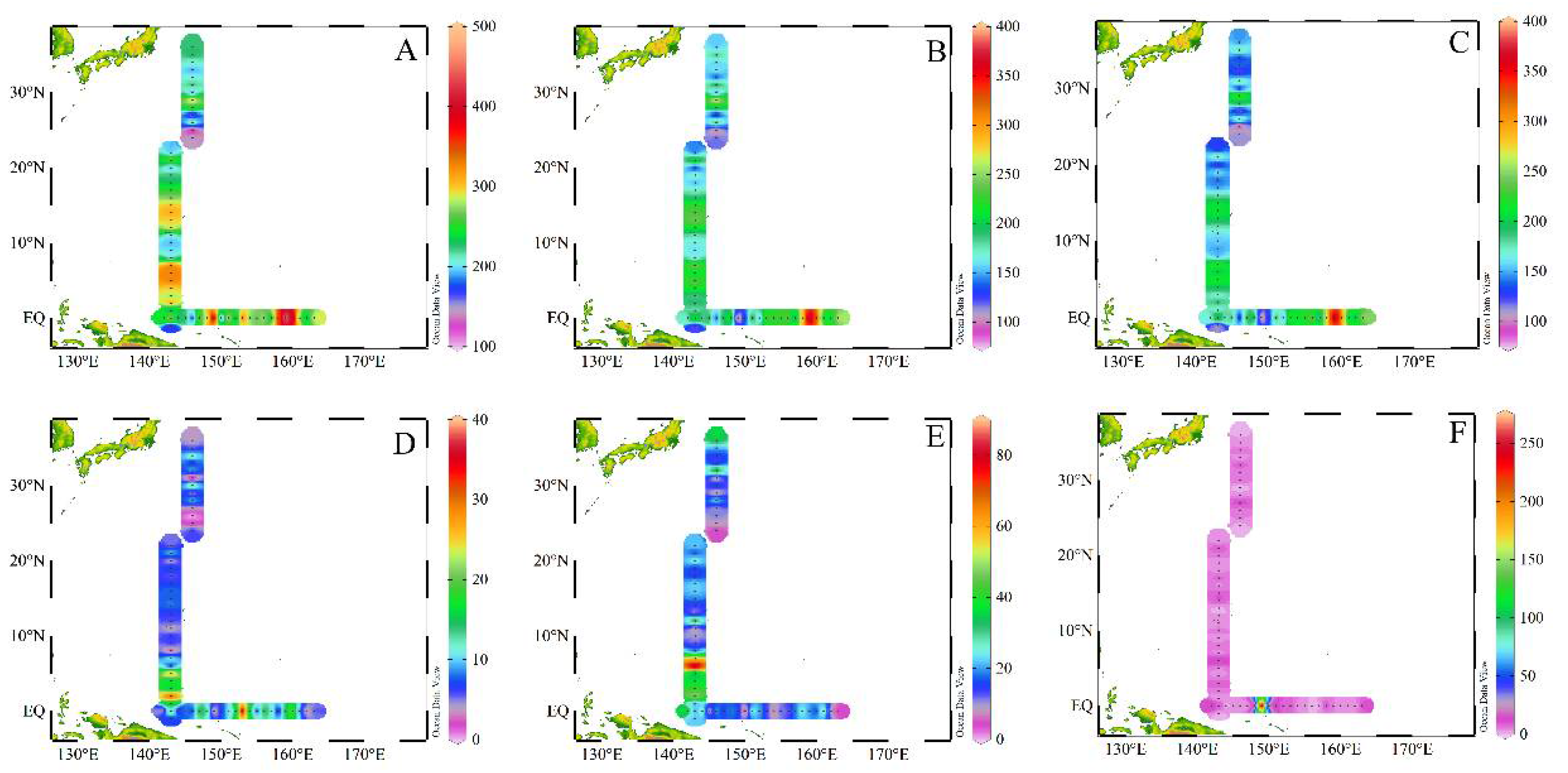
3.3. Zooplankton Abundance Distribution

The density of zooplankton in the surveyed area ranged from 118.3 to 452.2 ind./m3, with an average density of 253.3 ± 65.0 ind./m3. The abundance of zooplankton is shown in Figure 4. High abundance values are mainly observed in the NECC region and the eastern equatorial region, while low abundance values are found in the STCC region, which is similar to the findings of Yang et al [18]. Among the zooplankton, the density of copepods ranged from 88.7 to 383.8 ind./m3, with an average density of 180.2 ± 53.3 ind./m3, accounting for 71.1% of the total abundance of zooplankton. Therefore, the distribution of zooplankton was mainly determined by the copepods [17].
Among the three sections, only 310 species of zooplankton were identified on the S1 section, with an average abundance of 204.9 ± 45.7 ind./m3. A total of 364 species of zooplankton were identified on the S2 section, with an average abundance of 258.9 ± 52.6 ind./m3, and 346 species of zooplankton were identified on the S3 section, with an average abundance of 275.3 ± 52.6 ind./m3. The S2 section had the highest number of species, while the S3 section had the highest average abundance. The top ten dominant species for each cross-section are shown in Table 1. The three cross-sectional common dominant species were Acrocalanus gibber, Paracalanus aculeatus, Oncaea venusta, Canthocalanus pauper, and Oithona similis.

3.4. Diversity Indices of the Zooplankton Community

Different indices of biodiversity can express the diversity of a zooplankton community or assemblage in different ways, but the best way to evaluate the diversity of a community is to use these indices in combination [24]. In general, from the five selected diversity indices, the species richness has the same trend as the Margalef index, providing an initial indication of the diversity of communities in the surveyed sea area. On the other hand, the values of diversity index (H′) and Pielou’s Evenness Index (J) showed similar distribution. For instance, as shown in Figure 5, at stations ST0734 and ST0735, the values of S and Dm are modest and in the middle of the range, whereas H’, J, D, and abundance were higher. On the contrary, although the species density was high at ST0315 (Figure 5), all five parameters showed low diversity indices (circled in Figure 5), which was caused by the large enrichment of zooplankton larvae (especially copepod larvae) at this site. H′ and J reached maxima (4.40 and 0.65, respectively) at ST0742 in the eastern part of the equatorial section, indicating the stability of the ecosystem. However, there was no clear trend in the latitudinal distribution of zooplankton communities due to the complexity of the Western Pacific Gyre, especially the multiple and complex circulations that may be related to the oceanic environment in which they live. Overall, the community diversity at the equatorial section of the surveyed area was higher than the latitudinal sections.

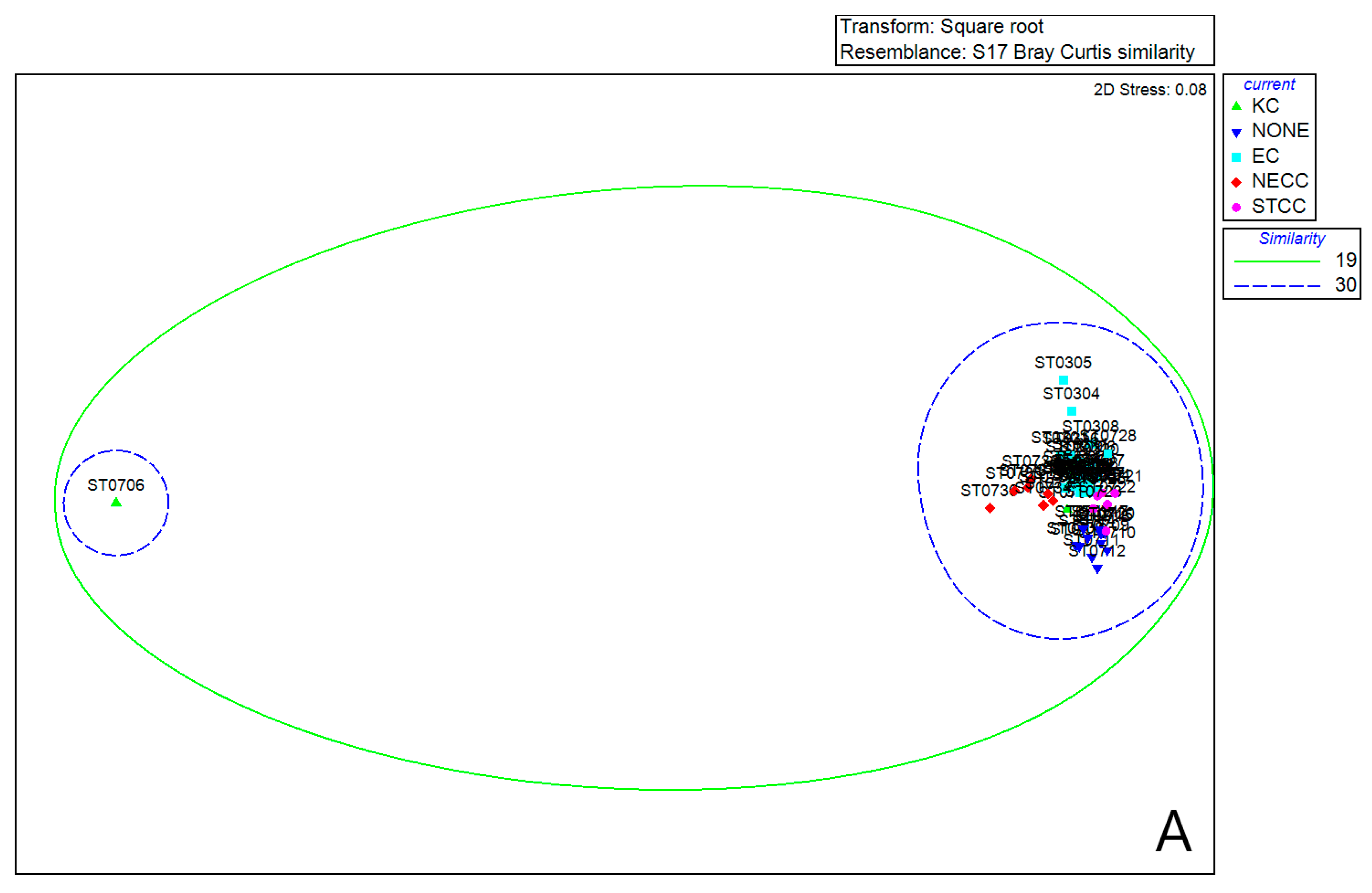
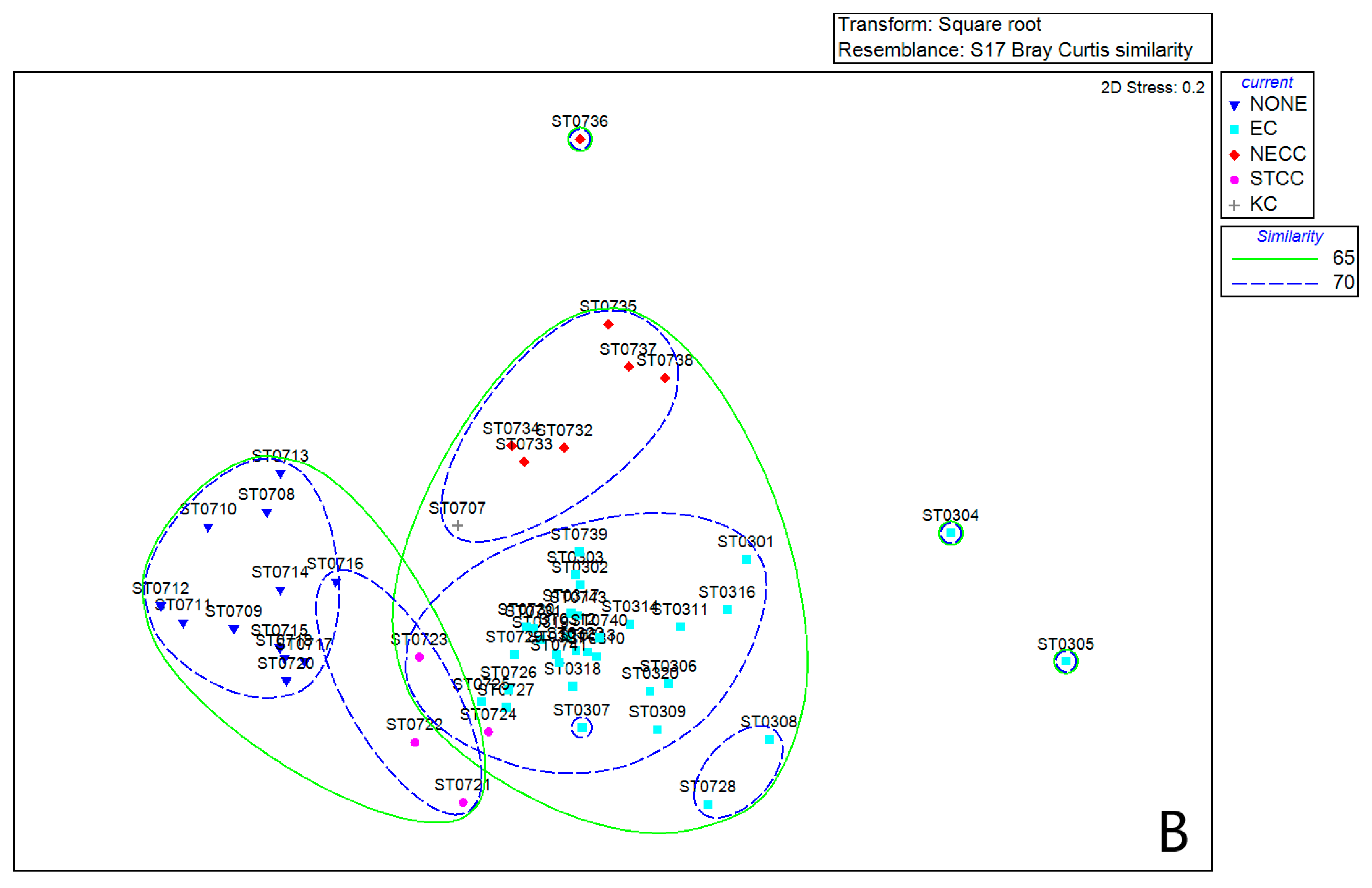
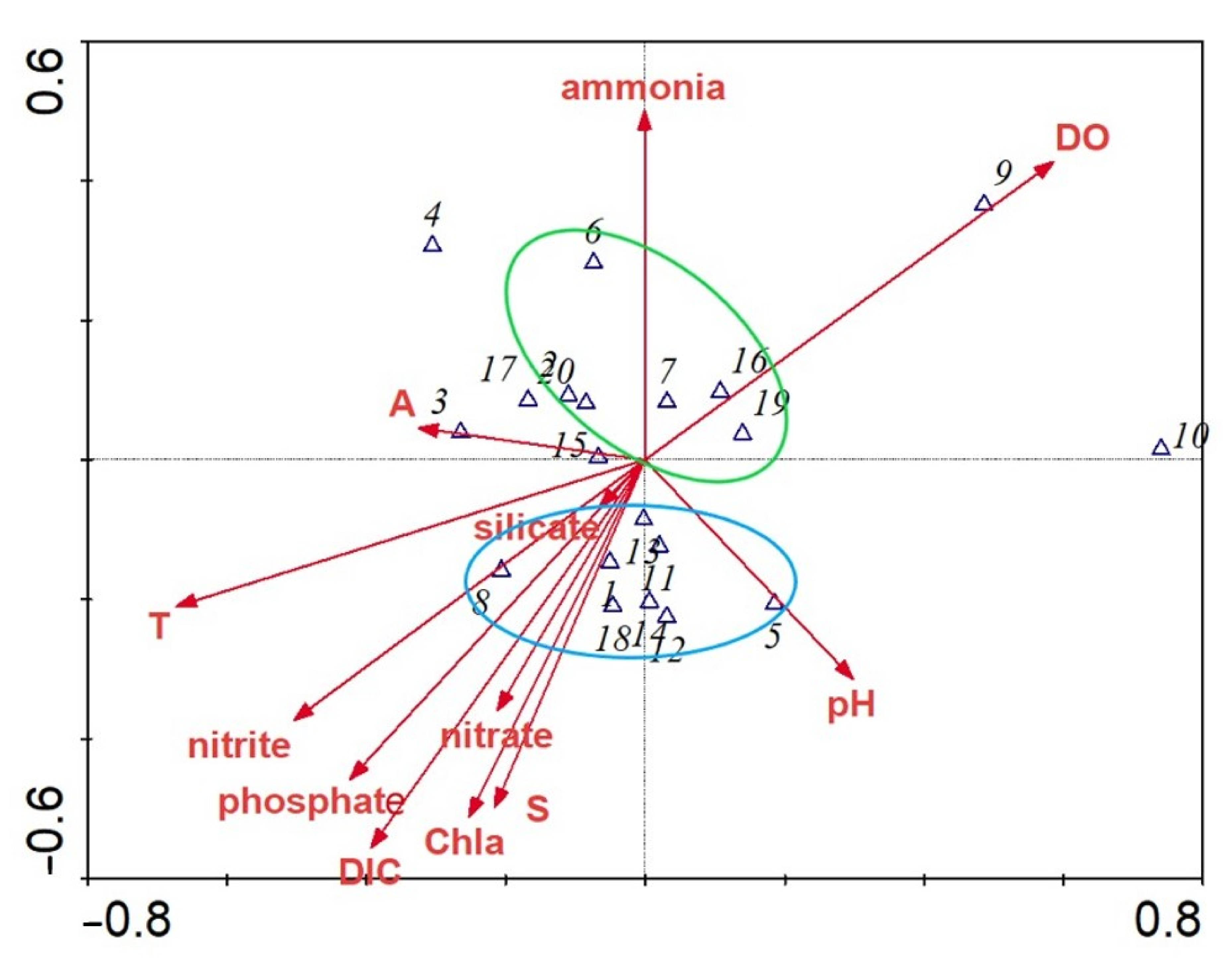
3.5. The Relationship between Zooplankton and the Environment

The results of the MDS analysis for all 59 samples are shown in Figure 6, in which station ST0706, affected by the KC, can be distinguished from the other stations according to a 30% similarity (Figure 6A). With the exception of station ST0706, the other stations were subjected to further MDS analysis, as shown in Figure 6B. Spatially, the zooplankton community group is more clearly influenced by the different circulations in the equatorial flow system when the similarity reaches 70%. The NECC group is clearly separate from the other groups, indicating that the zooplankton community structure of the NECC is significantly different from that of the other circulations. The STCC group is partially intersected with the EC group because both EC and STCC are flow systems with high transparency and STCC activity is reduced in the autumn [30]. The division of these groups indicates a strong link between zooplankton community structure and the circulation.
A comparative analysis of the organisms and the environment allows us to identify the key factors that influence zooplankton growth, which is vital for a healthy and stable ecosystem [31]. The CCA method was used to analyze the relationship between environmental parameters and dominant species, and the results are shown in Figure 7. The zooplankton community in this area can be roughly divided into two types, one associated with ammonium and dissolved oxygen (DO) (green circles) and the other with nutrients, chlorophyll a, and environmental factors. In addition, the growth of zooplankton can be closely related to nutrient. From Table 2 we can also see that zooplankton distribution was significantly correlated with nitrite and food (p < 0.05), while the total distribution of copepods was also significantly correlated with dissolved oxygen (DO) (p < 0.01). However, copepods differ according to environmental factors. For example, Clausocalanus arcuicornis is more biased toward high nitrite, and Lucicutia flavicornis is more biased toward high-dissolved-oxygen environments.

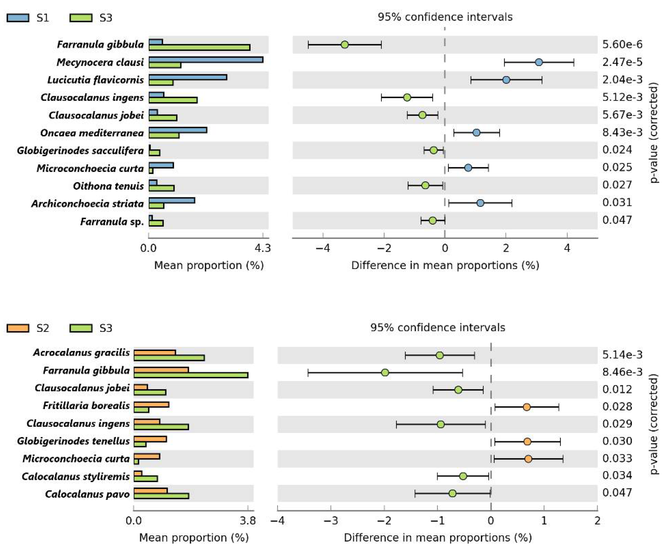
3.6. Comparison of Equatorial Zooplankton Communities with S1 and S2

In terms of total abundance, the zooplankton abundance in S3 is higher than that in S2, and the lowest abundance is in S1. However, this does not reveal the difference in zooplankton community structure between the equatorial and latitudinal segments well. Therefore, we selected the species with more than 30% occurrence between 59 stations to compare the abundance between the two groups (S3 and S1, S3 and S2). A total of 11 species of zooplankton were significantly different in abundance when comparing S3 with S1, while nine species were significantly different when comparing S3 with S2. The results of the significant (p < 0.05) differences in abundance between the two groups are shown in Figure 8. In both sets of comparisons, there were significant differences in abundance between the four species: Farranula gibbula, Clausocalanus ingens, Clausocalanus jobei, and Microconchoecia curta. Of these, Farranula gibbula had the greatest difference in abundance in both comparisons, with much greater abundance in S3 than in the other two transects.

4. Discussion

4.1. Comparison with Historical Data

Zooplankton diversity study in the Western Pacific Ocean is scarce and mostly concentrated in the South China Sea and around the Philippine Sea, while the open ocean and equatorial waters are less well studied [6]. The zooplankton abundance found in this research is within the range of values in the tropical and subtropical oceans [17,22,32]. Consistent with previous observations in tropical and subtropical regions, copepods, especially small copepods, make up the largest proportion of the zooplankton community [33]. This is also in line with observations in many other sea areas. This is due to the fact that small copepods have higher growth rates and have a large effect on the nutritional coupling between the upper and lower trophic levels [32,34]. They are better suited than large zooplankton to live in oligotrophic regions [35]. In contrast to previous studies, the area surveyed also includes the equatorial sea section. This may be one of the reasons why the number of species in the present study is somewhat higher than in the study of Dai et al. Similar to the findings of Dai et al. [17] and Yang et al. [18], copepods and Chaetognaths are the dominant taxa in the Western Pacific. However, as shown in Table 3, the zooplankton abundance in this survey was more consistent with the results of Yang et al. [18] and Sun et al. [19] and much higher than the results of Dai et al. [17]. This may be related to the different methods used in the survey [36,37]. In addition, as there is no absolute relationship between the diversity indices [31], the reasons for the high enrichment of zooplankton larvae (especially copepod larvae) in ST0315 need further study. Overall, compared to the studies of phytoplankton in the Western Pacific, the information on zooplankton in the Western Pacific is relatively scarce. Therefore, more survey material is needed to gain a full understanding of the biodiversity of the area.

4.2. Relationship between Ocean Current Factors and Zooplankton

Among the three transects surveyed in the study, S1 had the lowest mean zooplankton abundance and the lowest number of species. S2 had the highest number of species, but its abundance was lower than the S3 transect’s. In tropical and subtropical waters such as the eastern Indian Ocean, there have also been instances of high abundance of three cross-sectional co-dominant species, such as Paracalanus aculeatus, Oncaea venusta, Canthocalanus pauper, and Cosmocalanus darwinii [38,39].
From the temperature and nutrient distribution (Chen et al., unpublished), it was evident that mixed alternating water masses of Kuroshio edge and tide-friendly subduction occurred at 35° N to 36° N (Figure 2). In mixed surface waters, zooplankton abundance is likely to be greater due to advection of zooplankton into the region [40]. But since the northern end of the S1 section is located at the edge of a mixed water mass, the Kuroshio edge and Kuril cold subduction had less impact on zooplankton abundance in this area and did not play a significant role in promoting zooplankton growth. As seen in Figure 8, the zooplankton community structure at station ST0706 was less similar to the community structure at other stations. So, we suggest that the edge of the mixed water column affects the composition of the zooplankton community structure. The southern end of the S1 section is affected by the STCC region. Although the STCC vorticity is cyclical [41], the vorticity is weaker in October. However, zooplankton abundance was affected and was the lowest in the entire survey area, similar to the results of previous studies [18]. Section S2 straddles the equatorial flow system in the Western Pacific Ocean, with the northern end in the STCC region, which, together with the southern end of S1, forms the area of lowest zooplankton abundance in the entire area surveyed. There is a strong thermal leap in the lower NEC that limits the upwelling of nutrient-rich water below the leap, resulting in low salt levels in the upper leap [42]. It was the nutrient limitation that led to the low zooplankton abundance in the NEC region of the survey [43]. Zooplankton abundance was high around 3–10 °N (NECC region) and where considerable upwelling was observed (Figure 3). Peterson et al. demonstrated by a two-cell zonal circulation pattern according to which zooplankton abundance is highest where upwelling is strongest [44]. This survey is in line with these observations as the zooplankton abundance in the NECC region reaches its highest levels at the station with strong upwelling (6° to 7° N latitude). Furthermore, the influence of the upwelling probably affects the entire NECC region as the zooplankton community structure here differs from that in other circulating regions (Figure 6). For S1 and S2, zooplankton abundance was the highest in the NECC region and lowest in the STCC region, in agreement with the results of Yang et al. [18]. However, this is not consistent with the findings of Sun et al. [19] that community abundance generally increases with increasing latitude [19]. However, a decreasing value of zooplankton abundance between 20° N and 30° N can also be seen in the graphs in their study.

4.3. Relationship between Other Factors and Zooplankton

Changes in zooplankton community structure and abundance reflect the dynamics of the entire marine ecosystem. In particular, key species of zooplankton play a critical role in controlling the overall condition of the marine ecosystem [7]. The distribution of zooplankton communities is inextricably linked to environmental factors (abiotic factors) [45]. In this study, S3 was mainly distributed in the WPWP, and its mean temperature (26.5 °C) was higher than the other two cross-sections (S1: 20.7 °C and S2: 25.0 °C). Several copepod key species show a clear pattern linking temperature with their horizontal distribution. For example, as seen in Table 2, there is a significant positive correlation between F. gibbula and temperature (p < 0.01). That means that F. gibbula prefers a high-temperature marine environment. Therefore, the abundance of F. gibbula in the S3 section was significantly greater than in S1 and S2 (Figure 8); the same was true for C. ingens and C. jobei. This indicates that temperature is one of the important factors affecting the horizontal distribution of zooplankton [46]. In addition to temperature, nutrient salts also have an effect on the structure of the zooplankton community. Wen-Tseng et al. have also shown that L. flavicornis has a high abundance in high-nutrient waters close to KC [47]. In contrast, in the present investigation, Table 2 shows that L. flavicornis is significantly associated with phosphate, ammonium, and DIC, while in Figure 8 the abundance of L. flavicornis is significantly higher in S1 than in S3. This is most likely due to the influence of high-nutrient saline water at the northern station of the S1 section, brought about by KC.
As an intermediate part of the food chain [48], the distribution of zooplankton is also affected by competition, predation, and the abundance of prey [45,49]. Dagg [50] confirmed through model studies in the Gulf of Mexico that phytoplankton mortality due to grazing is always high and that more than 95% of grazing is caused by microzooplankton communities. White et al. [51] found a strong relationship between zooplankton biomass and phytoplankton growth rate. In our survey the high average abundance of the S3 section was largely dependent on high zooplankton abundance in the vicinity of station ST0305. Also, in this sea survey, the phytoplankton density was highest at station ST0305 [52]. In addition, although some species belong to the same genus, it is also possible that, as a result of differences in body size and other morphologies (e.g., mouthparts) between species, selection for the environment may vary, thus exhibiting different ecological taxa [53]. As shown in Figure 6 with the example of the genus Clausocalanus, C. furcatus is dominant in very oligotrophic waters, while C. acrcuicornis prefers salinity, which is consistent with the findings of Peralba et al. [53]. Thus, although they are both tropical species in the broad sense, they are indeed separate in terms of the population core [53], which confirms that they have different environmental preferences.
However, the distribution of zooplankton communities is closely linked not only to temperature and nutrients, but also to water masses and ocean circulation [54,55]. In comparison, our study is deficient in some relevant physical data. So, in future studies, physical data such as circulation and eddies should be included and reconciled to gain a more complete understanding of the zooplankton community distribution in this area.

5. Conclusions

The zooplankton community of three transects in the Western Pacific Ocean was investigated. The distribution of zooplankton differed significantly with the water currents. A total of 384 species of zooplankton adults were identified in this survey. The highest abundance of zooplankton was found in the NECC and equatorial regions, followed by the NEC region; the lowest abundance was in the STCC region. It was also found that the difference in the abundance of the species F. gibbula, C. ingens, and C. jobei between S3 and the other two cross-sections was mainly due to differences in temperature. Therefore, temperature influences the structure of the zooplankton community. In addition, nutrient concentrations, dissolved oxygen, and chlorophyll can influence the distribution of dominant species. Especially in the oligotrophic sea, small changes in nutrient concentrations can promote the proliferation of the zooplankton community. In this survey, we found that not only temperature and nutrient salinity, but also ocean currents and the movement of water masses influence the distribution of zooplankton communities in the Western Pacific.
Although this research provides baseline data and information, Western Pacific zooplankton still remain a mystery to us, especially the distribution of zooplankton throughout the water column and eddies. Therefore, more community-based and long-term studies are needed to further explore the role of zooplankton in marine biogeochemistry in the Western Pacific Ocean.

Author Contributions

Conceptualization, J.S.; Data curation, Y.L.; Formal analysis, Y.L.; Funding acquisition, J.S.; Investigation, Y.L. and D.C.; Resources, D.C., S.W., H.Y., H.C., and M.W.; Supervision, J.S.; Writing—original draft, Y.L.; Writing—review and editing, M.A.N. and J.S. All authors have read and agreed to the published version of the manuscript.

Funding

This research was supported by the National Key Research and Development Project of China (2019YFC1407805), the National Natural Science Foundation of China (41876134, 41676112, and 41276124), the Tianjin 131 Innovation Team Program (20180314), and the Changjiang Scholar Program of Chinese Ministry of Education (T2014253) to Jun Sun.

Institutional Review Board Statement

Not applicable.

Informed Consent Statement

Not applicable

Data Availability Statement

All data are available from the authors upon request.

Acknowledgments

We thank all the members of Dongfanghong 2 for supporting and securing our scientific investigation on this cruise. In addition, this work was supported by the National Key Research and Development Project of China (2019YFC1407805), the National Natural Science Foundation of China (41876134, 41676112 and 41276124), the Tianjin 131 Innovation Team Program (20180314), and the Changjiang Scholar Program of Chinese Ministry of Education (T2014253) to Jun Sun.

Conflicts of Interest

The authors declare no conflict of interest.

References

  1. Allain, V.; Fernandez, E.; Hoyle, S.D.; Caillot, S.; Juradomolina, J.; Andrefouet, S.; Nicol, S.J. Interaction between coastal and oceanic ecosystems of the Western and Central Pacific Ocean through predator-prey relationship studies. PLoS ONE 2012, 7, 1–9. [Google Scholar] [CrossRef] [PubMed] [Green Version]
  2. Morato, T.; Hoyle, S.D.; Allain, V.; Nicol, S.J. Seamounts are hotspots of pelagic biodiversity in the open ocean. Proc. Natl. Acad. Sci. USA 2010, 107, 9707–9711. [Google Scholar] [CrossRef] [PubMed] [Green Version]
  3. Longhurst, A.R. Chapter 11—The pacific ocean. In Ecological Geography of the Sea, 2nd ed.; Longhurst, A.R., Ed.; Academic Press: Burlington, MA, USA, 2007; pp. 327–441. [Google Scholar]
  4. Hu, S.; Hu, D. Review on western pacific warm pool study. Stud. Mar. Sin. 2016, 51, 37–48. (In Chinese) [Google Scholar]
  5. Grenier, M.; Cravatte, S.; Blanke, B.; Menkes, C.E.; Kochlarrouy, A.; Durand, F.; Melet, A.; Jeandel, C. From the western boundary currents to the Pacific Equatorial Undercurrent: Modeled pathways and water mass evolutions. J. Geophys. Res. 2011, 116, C12044. [Google Scholar] [CrossRef] [Green Version]
  6. Lin, M.; Wang, C.; Wang, Y.; Xiang, P.; Wang, Y.; Lian, G.; Chen, R.; Chen, X.; Ye, Y.; Dai, Y.; et al. Zooplanktonic diversity in the western Pacific. Biodivers. Sci. 2011, 19, 646–654. (In Chinese) [Google Scholar]
  7. Tittensor, D.P.; Mora, C.; Jetz, W.; Lotze, H.K.; Ricard, D.; Berghe, E.V.; Worm, B. Global patterns and predictors of marine biodiversity across taxa. Nature 2010, 466, 1098–1101. [Google Scholar] [CrossRef]
  8. Allen, G.R. Conservation hotspots of biodiversity and endemism for Indo—Pacific coral reef fishes. Aquat. Conserv. Mar. Freshwat. Ecosyst. 2008, 18, 541–556. [Google Scholar] [CrossRef]
  9. Briggs, J.C. The marine East Indies: Diversity and speciation. J. Biogeogr. 2005, 32, 1517–1522. [Google Scholar] [CrossRef]
  10. Karl, D.M. A sea of change: Biogeochemical variability in the North Pacific Subtropical Gyre. Ecosystems 1999, 2, 181–214. [Google Scholar] [CrossRef]
  11. Taniguchi, A. Phytoplankton-Zooplankton relationships in the western Pacific Ocean and adjacent seas. Mar. Biol. 1973, 21, 115–121. [Google Scholar] [CrossRef]
  12. Sun, J.; Liu, D.; Wang, Z.; Zhu, M. The effects of zooplankton grazing on the development of red tides. Acta Ecol. Sin. 2004, 24, 1514–1522. [Google Scholar]
  13. Calbet, A.; Landry, M.R. Phytoplankton growth, microzooplankton grazing, and carbon cycling in marine systems. Limnol. Oceanogr. 2004, 49, 51–57. [Google Scholar] [CrossRef] [Green Version]
  14. Sun, J.; Li, X.; Chen, J.; Guo, S. Progress in oceanic biological pump. Acta Oceanol. Sin. 2016, 38, 1–21. [Google Scholar] [CrossRef]
  15. Menkes, C.E.; Allain, V.; Rodier, M.; Gallois, F.; Lebourges-Dhaussy, A.; Hunt, B.P.V.; Smeti, H.; Pagano, M.; Josse, E.; Daroux, A.; et al. Seasonal oceanography from physics to micronekton in the south-west Pacific. Deep Sea Res. II 2015, 113, 125–144. [Google Scholar] [CrossRef] [Green Version]
  16. Houssem, S.; Marc, P.; Christophe, M.; Anne, L.-D.; Hunt, B.P.V.; Valerie, A.; Martine, R.; de Boissieu, F.; Elodie, K.; Cherif, S. Spatial and temporal variability of zooplankton off New Caledonia (Southwestern Pacific) from acoustics and net measurements. J. Geophys. Res. Ocean. 2015, 120, 2676–2700. [Google Scholar]
  17. Dai, L.; Li, C.; Sun, X.; Ji, P.; Zhang, W. Abundance and biomass of zooplankton in Philippine Sea in winter 2012. Oceanol. Limnol. Sin. 2014, 45, 1225–1233. (In Chinese) [Google Scholar]
  18. Yang, G.; Li, C.; Wang, Y.; Wang, X.; Dai, L.; Tao, Z.; Ji, P. Spatial variation of the zooplankton community in the western tropical Pacific Ocean during the summer of 2014. Cont. Shelf Res. 2017, 135, 14–22. [Google Scholar] [CrossRef]
  19. Sun, D.; Wang, C. Latitudinal distribution of zooplankton communities in the Western Pacific along 160° E during summer 2014. J. Mar. Syst. 2017, 169, 52–60. [Google Scholar] [CrossRef]
  20. Le Borgne, R.; Rodier, M. Net zooplankton and the biological pump: A comparison between the oligotrophic and mesotrophic equatorial Pacific. Deep Sea Res. II 1997, 44, 2003–2023. [Google Scholar]
  21. Roman, M.R.; Dam, H.G.; Gauzens, A.L.; Urban-Rich, J.; Foley, D.G.; Dickey, T.D. Zooplankton variability on the equator at 140° W during the JGOFS EqPac study. Deep Sea Res. II 1995, 42, 673–693. [Google Scholar] [CrossRef]
  22. Ishizaka, J.; Harada, K.; Ishikawa, K.; Kiyosawa, H.; Furusawa, H.; Watanabe, Y.; Ishida, H.; Suzuki, K.; Handa, N.; Takahashi, M. Size and taxonomic plankton community structure and carbon flow at the equator, 175‡E during 1990–1994. Deep Sea Res. II 1997, 44, 1927–1949. [Google Scholar] [CrossRef]
  23. Hu, D.; Wu, L.; Cai, W.; Gupta, A.S.; Ganachaud, A.; Qiu, B.; Gordon, A.L.; Lin, X.; Chen, Z.; Hu, S.; et al. Pacific western boundary currents and their roles in climate. Nature 2015, 522, 299–308. [Google Scholar] [CrossRef] [PubMed]
  24. Grasshoff, K.; Kremling, K.; Ehrhardt, M. Methods of Seawater Analysis, 3rd ed.; Wiley: Hoboken, NJ, USA, 1999. [Google Scholar]
  25. Sun, J.; Liu, D. The application of diversity indices in marine phytoplankton studies. Acta Oceanol. Sin. 2004, 26, 62–75. (In Chinese) [Google Scholar]
  26. Ma, C.; Wang, Z.; Zhou, E. Characteristics of currents in the west Pacific Ocean. Adv. Mar. Sci. 1983, 1, 24–36. [Google Scholar]
  27. Ganachaud, A.; Cravatte, S.; Melet, A.; Schiller, A.; Holbrook, N.J.; Sloyan, B.M.; Widlansky, M.J.; Bowen, M.; Verron, J.; Wiles, P.; et al. The Southwest Pacific Ocean circulation and climate experiment (SPICE). J. Geophys. Res. 2014, 119, 7660–7686. [Google Scholar] [CrossRef]
  28. Graham, N.E.; Barnett, T.P. Sea surface temperature, surface wind divergence, and convection over tropical oceans. Science 1987, 238, 657–659. [Google Scholar] [CrossRef] [PubMed]
  29. Bai, X.; Yang, F.; Dong, M.; Wu, Y.; Chen, H. The vertical distribution of nutrients in the upper water of the equatorial western Pacific Ocean in autumn. Period. Ocean Univ. China 2019, 49, 64–71. (In Chinese) [Google Scholar]
  30. Lan, S. Summery basic characteristics of temperature and salinity at 155° E section. Stud. Mar. Sin. 1999, 00, 1–11. [Google Scholar]
  31. Kobashi, F.; Kawamura, H. Seasonal variation and instability nature of the North Pacific Subtropical Countercurrent and the Hawaiian Lee Countercurrent. J. Geophys. Res. Ocean. 2002, 107, 6-1–6-18. [Google Scholar] [CrossRef]
  32. Liu, H.; Huang, Y.; Zhai, W.; Guo, S.; Jin, H.; Sun, J. Phytoplankton communities and its controlling factors in summer and autumn in the southern Yellow Sea, China. Acta Oceanol. Sin. 2015, 34, 114–123. [Google Scholar] [CrossRef]
  33. Neumann-Leitão, S.; Sant’anna, E.M.E.; Gusmão, L.M.D.O.; Do Nascimento-Vieira, D.A.; Paranaguá, M.N.; Schwamborn, R. Diversity and distribution of the mesozooplankton in the tropical Southwestern Atlantic. J. Plankton Res. 2008, 30, 795–805. [Google Scholar] [CrossRef]
  34. Chiba, S.; Batten, S.D.; Yoshiki, T.; Sasaki, Y.; Sasaoka, K.; Sugisaki, H.; Ichikawa, T. Temperature and zooplankton size structure: Climate control and basin-scale comparison in the North Pacific. Ecol. Evol. 2015, 5, 968–978. [Google Scholar] [CrossRef] [PubMed]
  35. Pielou, E.C. Mathematical Ecology, 2nd ed.; Wiley & Sons: New York, NY, USA, 1977; p. 47. [Google Scholar]
  36. Zervoudaki, S.; Christou, E.D.; Nielsen, T.G.; Siokoufrangou, I.; Assimakopoulou, G.; Giannakourou, A.; Maar, M.; Pagou, K.; Krasakopoulou, E.; Christaki, U. The importance of small-sized copepods in a frontal area of the Aegean Sea. J. Plankton Res. 2007, 29, 317–338. [Google Scholar]
  37. Hernroth, L. Sampling and filtration efficiency of two commonly used plankton nets. A comparative study of the Nansen net and the Unesco WP 2 net. J. Plankton Res. 1987, 9, 719–728. [Google Scholar] [CrossRef]
  38. Evans, M.S.; Sell, D.W. Mesh size and collection characteristics of 50-cm diameter conical plankton nets. Hydrobiologia 1985, 122, 97–104. [Google Scholar] [CrossRef]
  39. Wen-Tseng, L.; Chang-Tai, S.; Jiang-Shiou, H. Diel vertical migration of the planktonic copepods at an upwelling station north of Taiwan, western North Pacific. J. Plankton Res. 2004, 26, 89–97. [Google Scholar]
  40. Li, K.; Yin, J.; Huang, L.; Tan, Y.; Lin, Q. A comparison of the zooplankton community in the Bay of Bengal and South China Sea during April–May, 2010. J. Ocean Univ. China 2017, 16, 1206–1212. [Google Scholar] [CrossRef]
  41. Sabatini, M.; Reta, R.; Matano, R. Circulation and zooplankton biomass distribution over the southern Patagonian shelf during late summer. Cont. Shelf Res. 2004, 24, 1359–1373. [Google Scholar] [CrossRef]
  42. Qiu, B. Seasonal Eddy Field Modulation of the North Pacific Subtropical Countercurrent: TOPEX/Poseidon Observations and Theory. J. Phys. Oceanogr. 1999, 29, 2471–2486. [Google Scholar] [CrossRef]
  43. Feng, S.; Li, F.; Li, S. Introduction to Ocean Science; Higher Education Press: Beijing, China, 1999; pp. 167–172. [Google Scholar]
  44. Hidaka, K.; Kawaguchi, K.; Tanabe, T.; Takahashi, M.; Kubodera, T. Biomass and taxonomic composition of micronekton in the western tropical-subtropical Pacific. Fish. Oceanogr. 2010, 12, 112–125. [Google Scholar] [CrossRef]
  45. Peterson, W.T.; Miller, C.B.; Hutchinson, A. Zonation and maintenance of copepod populations in the Oregon upwelling zone. Deep Sea Res. Part A Oceanogr. Res. Pap. 1979, 26, 467–494. [Google Scholar] [CrossRef]
  46. Sommer, U. Plankton ecology: Succession in plankton communities. In Brock/Springer Series in Contemporary Bioscience; Springer: Berlin/Heidelberg, Germany, 1989. [Google Scholar]
  47. Zheng, Z. Introduction to Planktonology; Science Press: Beijing, China, 1964; pp. 78–81. [Google Scholar]
  48. Lo, W.-T.; Dahms, H.-U.; Hwang, J.-S. Water mass transport through the northern Bashi Channel in the northeastern South China Sea affects copepod assemblages of the Luzon Strait. Zool. Stud. 2014, 53, 66. [Google Scholar] [CrossRef]
  49. Banse, K. Zooplankton: Pivotal role in the control of ocean production: I. Biomass and production. ICES J. Mar. Sci. 1995, 52, 265–277. [Google Scholar] [CrossRef]
  50. Quintana, X.D.; Arim, M.; Badosa, A.; Blanco, J.M.; Boix, D.; Brucet, S.; Compte, J.; Egozcue, J.J.; de Eyto, E.; Gaedke, U.; et al. Predation and competition effects on the size diversity of aquatic communities. Aquat. Sci. 2015, 77, 45–57. [Google Scholar] [CrossRef]
  51. Dagg, M. Ingestion of phytoplankton by the micro- and mesozooplankton communities in a productive subtropical estuary. J. Plankton Res. 1995, 17, 845–857. [Google Scholar] [CrossRef]
  52. White, J.R.; Zhang, X.; Welling, L.A.; Roman, M.R.; Dam, H.G. Latitudinal gradients in zooplankton biomass in the tropical Pacific at 140° W during the JGOFS EqPac study: Effects of El Niño. Deep Sea Res. Part II 1995, 42, 715–733. [Google Scholar] [CrossRef]
  53. Chen, Z.; Sun, J. Effects of ocean currents in the western Pacific Ocean on net-phytoplankton. manuscript in preparation.
  54. Peralba, U.; Mazzocchi, M.G.; Harris, R.P. Niche separation and reproduction of Clausocalanus species (Copepoda, Calanoida) in the Atlantic Ocean. Prog. Oceanogr. 2017, 158, 185–202. [Google Scholar] [CrossRef]
  55. Huang, B.; Wu, J.; Tang, J.; Hu, J.; Wang, J. The study on the correlation between zooplankton community and water mass in the Hangzhou Bay. Acta Oceanol. Sin. 2010, 32, 170–175. (In Chinese) [Google Scholar]
Figure 1. Sampling stations of the 2017 Western Pacific Cruise; the appropriate locations of the different currents are described according to Hu et al. and categorized into S1, S2, and S3 transects based on the shadow environment of the station circulation. Surface currents include the Kuroshio Current (KC), Subtropical Countercurrent (STCC), Northern Equatorial Current (NEC), North Equatorial Countercurrent (NECC), and Equatorial Undercurrent (EUC).
Diversity 13 00058 g001
Figure 2. Integral distribution of the water column for temperature and salinity. (A) Temperature (°C); (B) salinity.
Diversity 13 00058 g002
Figure 3. The transection distribution of temperature (°C) and salinity. (A1A3) represents the temperature of S1, S2, and S3 and (B1B3) represents the salinity of S1, S2, and S3.
Diversity 13 00058 g003
Figure 4. The horizontal surface distribution of zooplanktons in the survey area (ind./m3). (AF) Species abundance, Arthropoda, Copepods, Chaetognaths, Chordata, and Larvae.
Diversity 13 00058 g004
Figure 5. The horizontal distribution of zooplankton species diversity indices. (AE) Species richness (S), Shannon–Wiener diversity index (H′), Pielou’s evenness index (J), Simpson’s diversity index (D), and Margalef’s diversity index (Dm). The circled station stands for ST0315.
Diversity 13 00058 g005
Figure 6. The results of a multidimensional scale analysis (MDS) of samples. (A) All 59 samples; (B) 58 samples—all but station ST0706.
Diversity 13 00058 g006aDiversity 13 00058 g006b
Figure 7. A canonical analysis of biotic and abiotic variables in the survey area. T represents temperature; S represents salinity; A represents total alkalinity; 1–20 are as follows: 1—Acartia negligens, 2—Canthocalanus pauper, 3—Cosmocalanus darwinii, 4—Nannocalanus minor, 5Calocalanus pavo, 6—Clausocalanus furcatus, 7—Clausocalanus farrani, 8—Clausocalanus arcuicornis, 9—Lucicutia flavicornis, 10—Mecynocera clausi, 11—Acrocalanus gibber, 12—Acrocalanus gracilis, 13—Paracalanus aculeatus, 14—Paracalanus gracilis, 15—Paracalanus parvus, 16—Parvocalanus crassirostris, 17—Parvocalanus elegans, 18—Oithona plumifera, 19—Oithona setigera, and 20—Oithona similis.
Diversity 13 00058 g007
Figure 8. Analysis of species abundance differences between equatorial sections (S3) and two latitudinal sections (S1 and S2).
Diversity 13 00058 g008
Table 1. Temperature, salinity, and dominant species in the S1, S2, and S3 cross-sections.
Section
S1S2S3
Location146° E, 24–36° N143° E, –1°–22° N0° N, 142–163° E
Temperature (°C)13.24–23.2013.24–23.2013.24–23.20
Salinity34.12–35.0633.65–35.0034.88–35.34
The top 10
dominant
species
(order of dominance from greatest to least)
Acrocalanus gibberAcrocalanus gibberAcrocalanus gracilis
Paracalanus aculeatusCanthocalanus pauperParacalanus aculeatus
Mecynocera clausiOithona similisFarranula gibbula
Oncaea venustaParacalanus aculeatusCanthocalanus pauper
Canthocalanus pauperOncaea venustaOncaea venusta
Oithona similisNannocalanus minorOithona similis
Lucicutia flavicornisClausocalanus furcatusAcrocalanus gibber
Oncaea mediterraneaFarranula concinnaAcartia negligens
Parvocalanus crassirostrisCosmocalanus darwiniiCosmocalanus darwinii
Acrocalanus graciliFarranula rostrataOithona plumifera
Table 2. The Pearson correlation coefficients between biotic and abiotic variables in the survey area.
SpeciesDOpHSilicatePhosphateNitriteNitrateAmmoniaDICTemperatureChl. a
H’−0.1980.245−0.0180.1140.280 *0.062−0.1950.0500.2220.314 *
J−0.2520.2220.0280.1780.260 *0.131−0.1800.1040.2000.319 *
Copepods−0.348 **0.057−0.0010.2490.495 **0.127−0.0580.2170.325 *0.528 **
Canthocalanus pauper−0.246−0.1480.0470.1680.2330.1190.0530.1320.2380.244
Cosmocalanus darwinii−0.200−0.0400.0530.1850.2320.118−0.0590.1470.2100.314 *
Calocalanus pavo−0.1180.269 *−0.0700.0930.0750.057−0.1770.0920.1050.230
Clausocalanus arcuicornis−0.274 *0.0940.0000.2130.418 **0.101−0.0210.285 *0.2210.420 **
Lucicutia flavicornis0.285 *0.088−0.145−0.289 *−0.070−0.2220.331 *−0.263 *−0.254−0.075
Acrocalanus gibber−0.337 **−0.0110.1090.309 *0.427 **0.246−0.0640.319 *0.1330.486
Paracalanus aculeatus−0.275 *0.1430.0550.263 *0.369 **0.188−0.0830.332 *0.1640.427
Oithona similis−0.130−0.0690.0430.1310.413 **0.0680.0410.0840.1690.295
Farranula gibbula−0.34**0.065−0.0780.2010.2860.08 *−0.1430.2070.487 **0.249
Clausocalanus ingens−0.364**0.077−0.0140.02520.465**0.162−0.0440.268 *0.298 *0.465 **
Clausocalanus jobei−0.316*0.0480.0780.02420.349**0.159−0.170.278 *0.289 *0.27 *
Note: * and ** represent significance at p < 0.05 and p < 0.01, respectively.
Table 3. The comparison of zooplankton with the historical data.
TimeResearch AreaReferences Method and Nesh SizeDepthNumber of Species and LarvaeAbundance
(ind./m3)
Reference
Nov.–Dec. 2012120–130° E,
0–20° N
ZooScan
500 um
0–200 m-11–116Dai et al. [17]
Aug.–Oct. 2014120°–135° E,
0–20°N
Microscope
200 um
0–300 m259Subregional average: 86.09–311.98Yang et al. [18]
June–July
2014
160° E
4°S–46° N
Microscope
200 um
0–200 m49845.11–439.84Sun et al. [19]
Oct.–Dec. 2017142–164° E,
–1–36° N
Microscope
200 um
0–200 m405118.33–452.22this study
Publisher’s Note: MDPI stays neutral with regard to jurisdictional claims in published maps and institutional affiliations.

