
Seasonal Shift of a Phytoplankton (>5 µm) Community in Bohai Sea and the Adjacent Yellow Sea


1
Research Centre for Indian Ocean Ecosystem, Tianjin University of Science and Technology, Tianjin 300457, China
2
College of Marine Science and Technology, China University of Geosciences (Wuhan), Wuhan 430074, China
3
Institute of Marine Science and Technology, Shandong University, 72 Binhai Road, Qingdao 266200, China
4
College of Biotechnology, Tianjin University of Science and Technology, Tianjin 300457, China
*
Author to whom correspondence should be addressed.
Diversity 2021, 13(2), 65; https://0-doi-org.brum.beds.ac.uk/10.3390/d13020065
Submission received: 22 October 2020
/
Revised: 29 January 2021
/
Accepted: 2 February 2021
/
Published: 5 February 2021
(This article belongs to the Special Issue Linking Plankton Diversity with Ecosystem Functioning and Services)
Abstract
:In order to better understand the seasonal variations in the phytoplankton community structure in the Bohai Sea (BS) and the North Yellow Sea (NYS), we carried out three cruises during 12 to 24 April 2019, 8 to 18 June 2019, and 12 to 22 October 2019. A total of 212 taxa (75 genera and three phyla) were identified, among which 83 taxa in 40 genera, 96 taxa in 43 genera, and 151 taxa in 62 genera were found in spring, summer, and autumn, respectively. Diatoms including Paralia sulcata and Coscinodiscus granii were the most dominant phytoplankton group during the three seasons, while several species of dinoflagellates, e.g., Scrippsiella troichoidea, Tripos massiliensis f. armatus, Gyrodinium spirale, and Prorocentrum minimum were found in warmer, saltier, and nutrient-poor waters. The diversity index of phytoplankton community was highest in autumn and lowest in summer. Based on cluster and multidimensional scaling analyses, the phytoplankton community of the BS and the NYS was divided into three ecological provinces: the BS, the coastal area, and the NYS. These three ecological provinces differed in physicochemical properties induced by the complicated water masses and circulations. Due to the influence of nutrient concentration, the phytoplankton diversity had the highest value in autumn, followed by spring, and the smallest in summer.
1. Introduction
The response of phytoplankton species composition to physical forcing may explain the ecological characteristics in the marine environment [1]. Marine phytoplankton are the primary producers, accounting for approximately 50% of the global net primary production [2,3]. They can influence the abundance and diversity of marine organisms and can also drive and reflect ecological functions [4]. Furthermore, phytoplankton can rapidly respond to environmental changes, and can be used as indicators of changes in marine environmental conditions [5]. One study [6] demonstrated that the dominant phytoplankton species composition in the East China Sea has changed in response to the variation in environmental conditions of coastal ecosystem among seasons, with most dinoflagellate species decreasing during autumn and winter compared to spring and summer.
Ecological provinces are regions with similar physical characteristics including water depth, temperature, salinity, and biological features [7,8]. Longhurst divided the global ocean into several regions based on ecological conditions for the first time [9,10]. Based on the sea surface temperature (SST) and Chl-a concentration obtained through satellite observations, Platt et al. [7] divided the Northwest Atlantic Ocean into multiple provinces to illustrate the influence of physical factors on phytoplankton species composition. Devred et al. [8] explained how to develop the relationship between biological activity and gas exchange using the method of ecological provinces based on temperature and fluorometry in northwest Atlantic. Taylor et al. [11] defined the bio-optical provinces using a cluster algorithm in the eastern Atlantic Ocean and pointed out the necessity for dynamic methods to reach consensus with established provinces. Although it has become a widely accepted tool for analyzing phytoplankton species composition and related biogeochemistry, the establishment of an ecological province has rarely been used to study the Bohai Sea (BS) and Yellow Sea (YS).
The BS and YS are semi-enclosed shelf seas located in northern China. Annually, complex oceanic circulations of water masses generate in the BS and YS, such as the Bohai Sea Mixed Water (BSMW), the Bohai Sea Southern Coastal Water (BSSCW), the Yellow Sea Cold Water Mass (YSCWM), the Yellow Sea Warm Current (YSWC), and the Yellow Sea Coastal Water (YSCW) [12,13]. Due to the changes in circulations, complex hydrographic conditions emerge in this area [14,15]. In the BS, the diversity of the phytoplankton community is low and uneven, and mainly concentrates to the BS strait [16]. Since the early 1950s, a series of phytoplankton taxonomy and ecology studies have been conducted in BS and YS [17]. Many studies have been carried on the relationship among nutrient dynamics, phytoplankton species composition, seasonal variation and cell abundance [18,19,20,21,22]. Despite the extensive study of the phytoplankton species composition in BS and YS, ecological provinces in phytoplankton species composition have not yet been defined.
Although numerous studies regarding the relationship between the environment and phytoplankton community have been carried out for several decades, there are few investigations on how the environment factors in different seasons influence the phytoplankton communities and their distributions [23]. In order to better understand the changes of phytoplankton communities and distributions in different areas and seasons, we studied the phytoplankton community (abundance, composition, and spatial distribution) in the BS and the North Yellow Sea (NYS) in three seasons: spring, summer, and autumn. Furthermore, we explored how different environmental parameters were associated with the seasonal changes of the phytoplankton community.
2. Materials and methods
2.1. Sampling Area
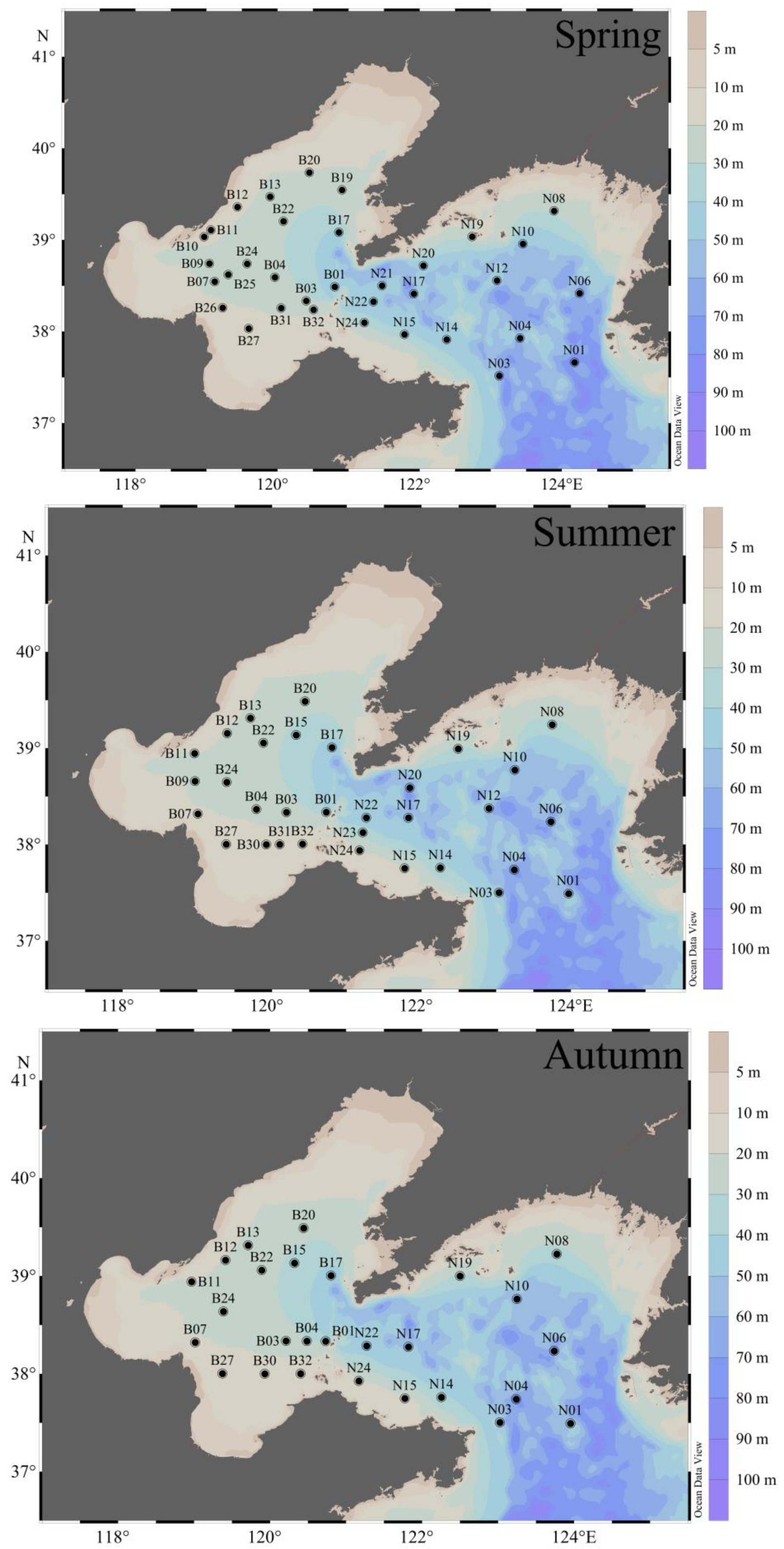
During 2019, we conducted three cruises in the BS and the NYS (37°–39.5° N, 118.5°–124.5° E) (Figure 1) and the BS and NYS were semi-enclosed shelf seas located in northern China: 12 to 24 April 2019, 8 to 18 June 2019, and 12 to 22 October 2019, representing spring, summer, and autumn, respectively. During these cruises, a total of 279 water samples in surface, bottom and bottom layers at 93 sampling stations were investigated.
2.2. Sampling and Analysis Methods
Water samples were collected with 12 Go-Flo bottles equipped with a SeaBird CTD (SBE 9/11 plus) and temperature, salinity, and pressure were recorded at the same time. The depth of the water samples is shown in Table 1 and defined as surface, middle, and bottom layers. The water samples for phytoplankton analysis were taken into 250 mL polyethylene (PE) bottles and quickly fixed with buffered formalin (1% of final concentration) and then stored in darkness. After returning to the laboratory, water samples were concentrated with 100 mL settlement columns for 24 to 48 h. Phytoplankton cells (cell size > 5 µm) were identified and counted under an inverted microscope (Motic BA300) at 400× (or 200×) magnification on the basis of the methodology described by Utermöhl [24]. We identified the phytoplankton taxonomy according to the methods of Jin et al. [25], Yamaji [26], and Sun [18].
The water samples for nutrient analysis were filtered through 0.45 µm cellulose acetate membrane filters and stored for further analysis in PE bottles, which had been cleaned by hydrochloric acid solution with volume ratio of 1:5 (HCl:H2O), and then refrigerated −20 °C for nutrient concentrations (NO3−-N, NO2−-N, PO43−-P, NH4+ and SiO32−-Si) were determined by a nutrient analyzer AA3 Auto-Analyzer (Bran + Luebbe) according to the colorimetric methods [27].
2.3. Data analysis and Statistical Methods
Phytoplankton community diversity was calculated according to the Shannon–Wiener (S–W) diversity index (H’) [28,29]:
where Pi represents the relative cell abundance of a species, i represents the numbers of the species, S represents the number of total species of phytoplankton in the samples collected. The evenness index (J) [30] was calculated by H’ [29] as follows:
The phytoplankton dominance index (Yi) was calculated by the following formula [31]:
where N is the total number of individuals in the collected samples, ni is the cell number of species i, fi is the frequency of occurrence of species i in each sample. The Jaccard similarity index (P) was calculated using the following formula [32]:
where a and b are the numbers of species in the BS and NYS, respectively, in two different seasons, and c is the number of the common species in the two different seasons.
The abundance of phytoplankton cells in water column was calculated through the trapezoidal integral method [33]:
where P’ is the average value of phytoplankton abundance in water column, Pi is the abundance value of phytoplankton in layer i, i + 1 is the layer i + 1, Dn is the maximum sampling depth, Di is the depth of layer i, and n is the sampling level.
Multidimensional scaling (MDS) and cluster analysis were performed using PRIMER 6.0 to reveal spatial patterns in the community composition [34]. In order to avoid the impact of rare species on the community, species with a dominance index (Y) < 0.09% were strictly excluded in MDS and cluster analysis. Canonical Correspondence Analysis (CCA) was performed using MVSP software (v 3.1.3), and was applied on log(x + 1) converted phytoplankton abundance and environmental data to determine the relationship between environmental parameters and the community composition [35]. The Ocean data view (4.6.7) and Grapher 10 were used to construct a graph depicting the sea surface and vertical distribution of phytoplankton abundance.
3. Results
3.1. Hydrographic Conditions
The water temperature and salinity from surface layer to bottom layer in the BS and NYS are shown in Figure 2. In spring, water temperature ranged from 5.1 to 13.1 °C (mean = 9.2 ± 1.7 °C), and the salinity ranged from 28.7 to 32.4 (mean = 31.8 ± 0.8). In summer, the sea surface temperature reached its maximum, among which the average temperature was 22.7 ± 3.8 °C (range 17.8–29.4 °C) and the average salinity was 31.6 ± 0.9 in the BS. In NYS, lower temperature and higher salinity were found, water temperature ranged from 6.8 to 27.4 °C (mean = 17.4 ± 7.0 °C) and salinity values (mean = 31.9 ± 0.4) varied between 30.7 and 32.6. In autumn, water temperature values (mean = 17.4 ± 3.0 °C) varied between 10.1 °C and 20.8 °C and small-scale salinity differences was observed in the NYS. No obvious difference in temperature was found in the BS, but the sea surface salinity values (mean = 31.4 ± 0.7) ranged from 29.9 to 32.1.
3.2. Species Composition
A total of 212 phytoplankton taxa were identified during the three cruises in the BS and NYS, belonging to three phyla and 75 genera, and the number of phytoplankton was highest in autumn. Among them, 83 species of 40 genera were identified in spring, 96 species belonging to 43 genera were identified in summer, and 151 species of 62 genera were identified in autumn, all these species belonged to three phyla involving Bacillariophyta, Pyrrhophyta, and Chrysophyta. Bacillariophyta were the most diverse group, and 108 diatom species were identified, Pyrrophyta was the second most diverse group (101 species) and species in Chrysophyta were recorded more sporadically, including three species in one genus. We obtained the top 15 dominant species of the phytoplankton community in each season by calculating the dominance index (Table 2 and Figure 3).
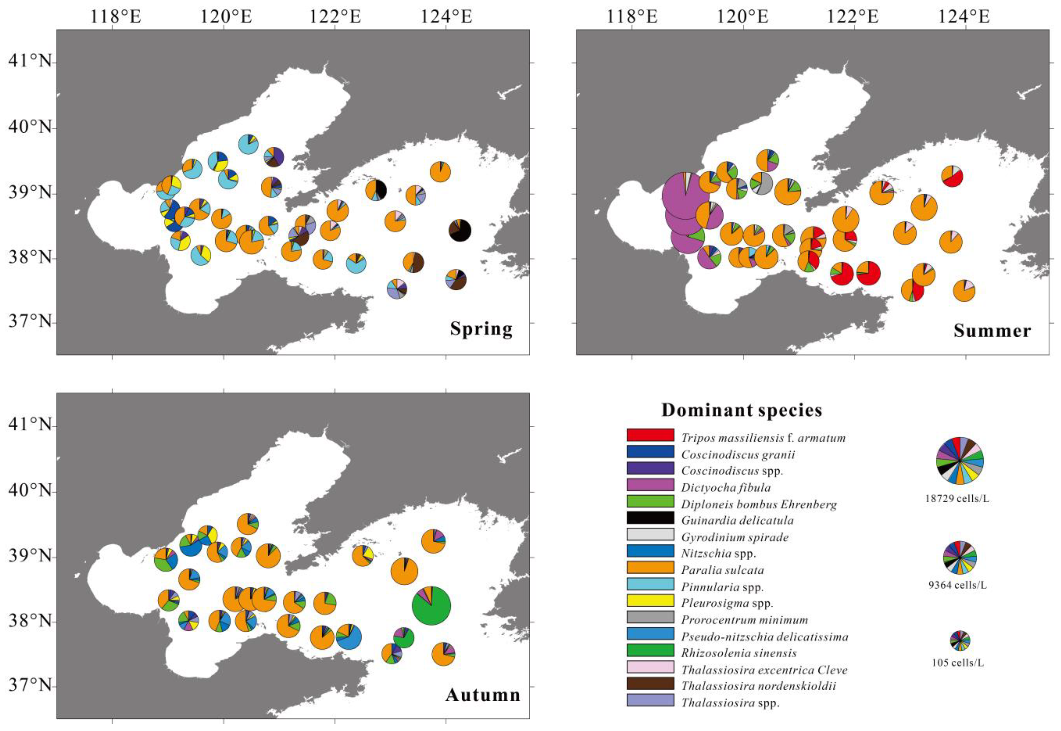
In spring, the dominant taxa belonged to diatoms and dinoflagellates in the BS and NYS. Dinoflagellates occurred in low numbers, representing 4.60% of the total cell abundance. Diatoms, chrysophytas, and dinoflagellates were the dominant groups in summer, the most abundant diatom species was Paralia sulcata. Other species such as Dictyocha fibula and Tripos massiliensis f. armatus, and Gyrodinium spirale were also relatively abundant. In autumn, no dinoflagellate was among the 15 most abundant species and the diatoms account for 95.85% of total phytoplankton abundance in autumn. The dominant species in the BS and NYS were diatoms, with Paralia sulcata, Coscinodiscus granii and Thalassiosira spp. being the common dominant species in the three seasons (Table 1). In addition, Dictyocha fibula decreased in autumn compared to summer.
There were 44–56 species among the three seasons in three cruises in all study area. The Jaccard similarity index values ranged between 0.29 and 0.34 (Table 3), with the highest level detected between spring and summer. This indicates that there were obvious seasonal variations in the phytoplankton community structure. The diversity index and evenness index of phytoplankton community was highest in autumn and lowest in summer (Table 4).
3.3. Sea Surface Distribution of Phytoplankton
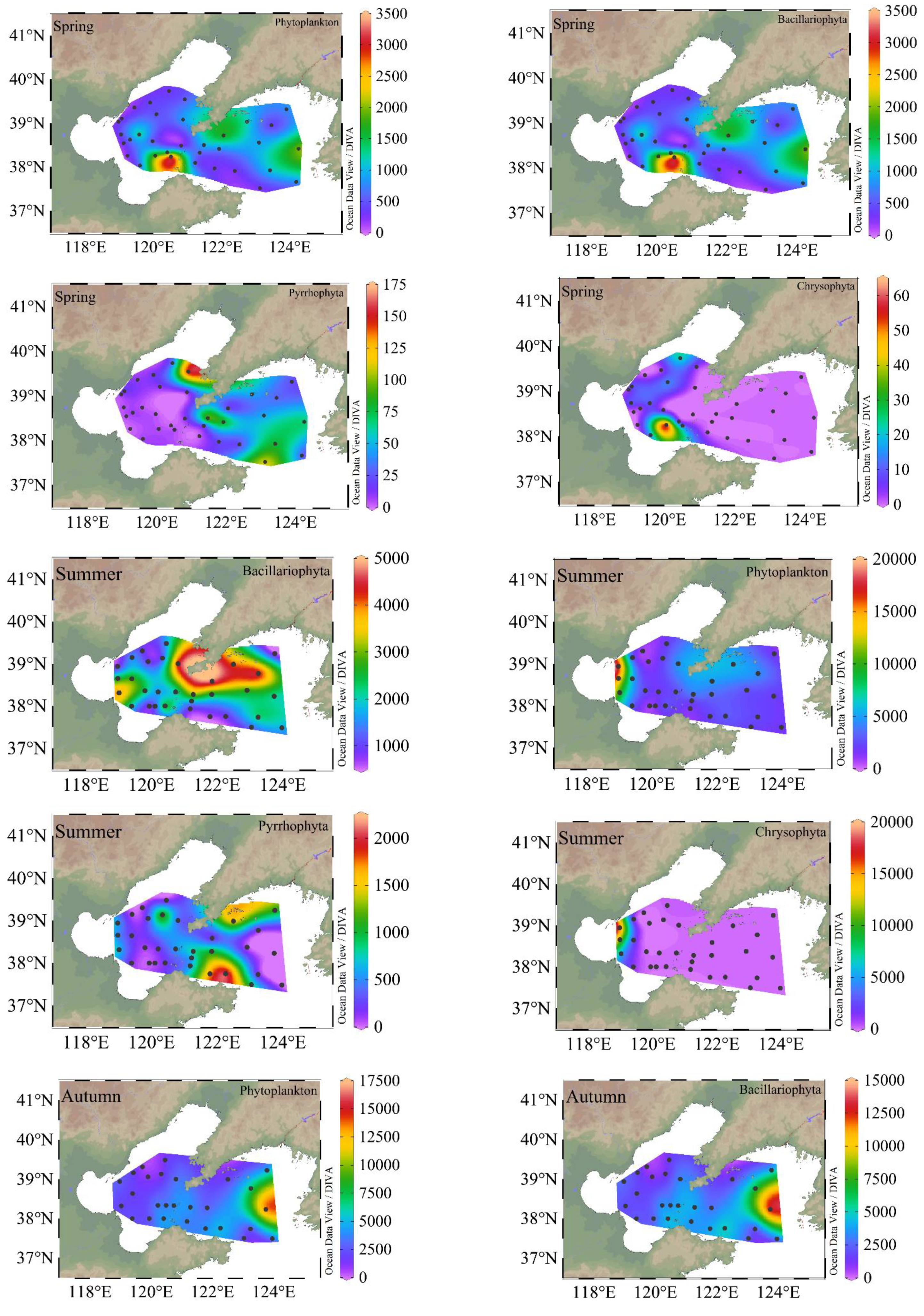
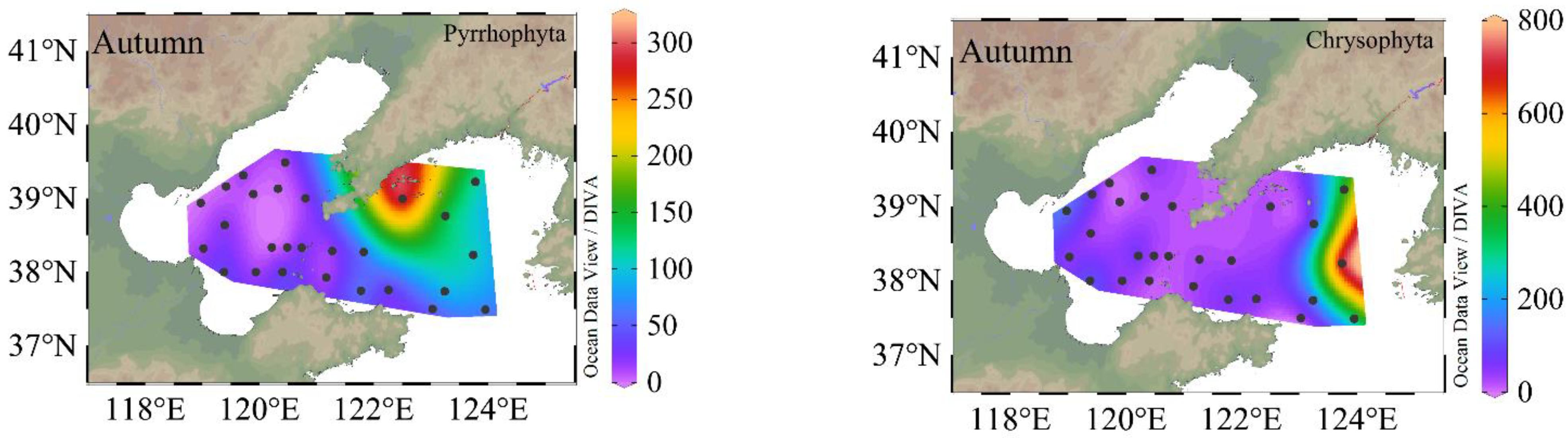
The sea surface distribution of phytoplankton, diatoms, dinoflagellates, and chrysophytas are shown in Figure 4. In the BS and NYS, the phytoplankton abundances ranged from 20 to 4.04 × 10³ cells·L−1, and the diatoms accounted for 95% of the total phytoplankton abundance. The relative abundance of dinoflagellates was usually low, accounting for 4.5% of the total cell abundance. In summer, the phytoplankton abundance was highest, ranging from 20 to 7.70 × 10⁴ cells·L−1, and consisted mainly of diatoms, dinoflagellates and chrysophytes. In autumn, the abundance of phytoplankton decreased ranging 20–2.91 × 10⁴ cells·L−1. In autumn, similar to spring, the phytoplankton abundance was mainly dominated by diatoms. The highest abundance of phytoplankton was found in the NYS.
3.4. Phytoplankton Assemblages Analysis and MDS
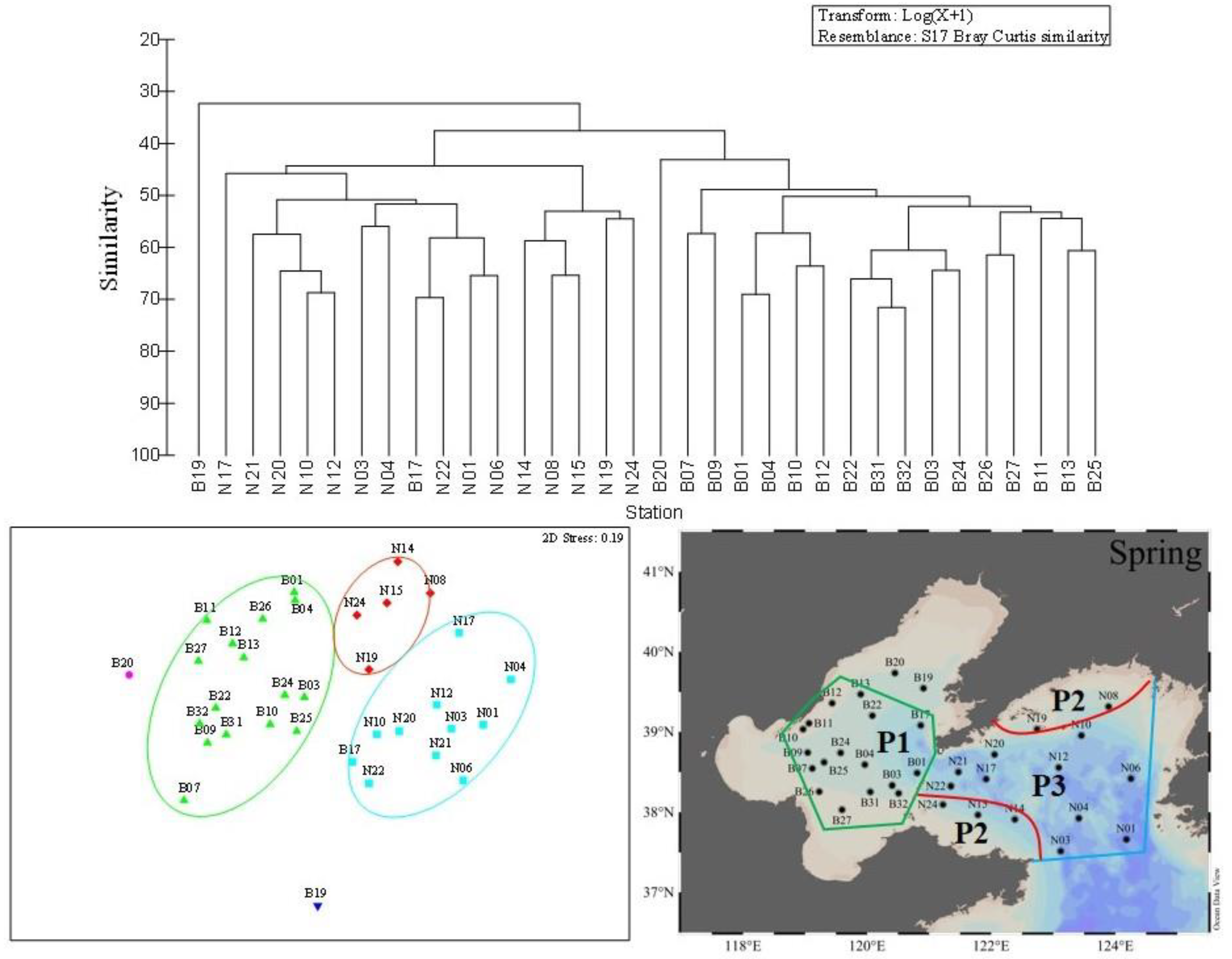
The dominance of phytoplankton taxa per season in the BS and NYS is presented in in Table 2. According to the abundance of the phytoplankton community as biological factors, the phytoplankton community could be classified into 3 ecological provinces based on MDS and cluster analysis (similarity 50%) in each season.
In spring, the first province consisted of 17 stations (Figure 5) which were mainly located in the BS (Figure 5). The average value of temperature and salinity were 10.2 ± 1.3 °C and 31.5 ± 1.0, respectively. The total phytoplankton abundance varied between 20 and 4 × 10³ cells·L−1, with an average value of 7.03 × 10² cells·L−1. The second province occurred at six stations (Figure 5). These stations mainly distributed in the coastal areas of NYS (Figure 5), and the average values of temperature and salinity were 8.9 ± 1.8 °C and 31.8 ± 0.1, respectively. The total phytoplankton abundance ranged from 80–1.81 × 10³ cells·L−1, with an average value of 5.63 × 10² cells·L−1. The third province was found at ten offshore stations in NYS (Figure 5). The mean values of temperature and salinity were 8.1 ± 1.6 °C and 31.8 ± 0.1, respectively. The general phytoplankton abundance varied from 30–3.15 × 10³ cells·L−1, and the mean value was 8.47 × 10² cells·L−1. In these three ecological provinces, diatoms dominated throughout the BS and NYS, and accounted for 98.9%, 93.0%, and 92.6% of the total phytoplankton abundance in each assemblage.
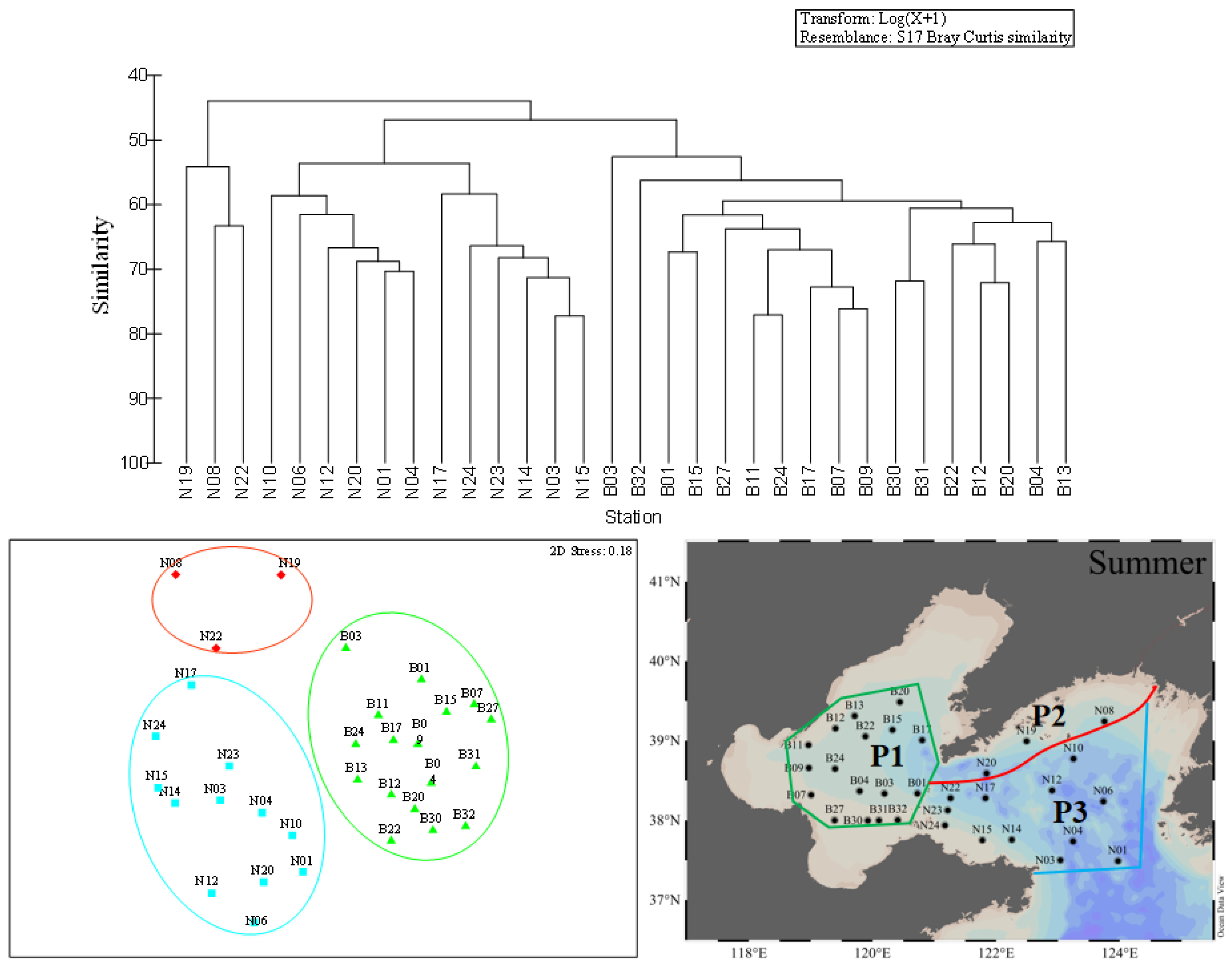
In summer, the first province was the same as the first province in spring and consisted by all stations in BS (Figure 6). The temperature and salinity were recorded with the mean values of 22.7 ± 3.8 °C and 31.3 ± 1.2, respectively. The general phytoplankton abundance was higher than other areas and varied from 1.40 × 10² to 7.70 × 10⁴ cells·L−1, with an average value of 5.3 × 10³ cells·L−1. Diatoms and chrysophytas accounted for 34.7% and 58.2% of the total phytoplankton abundance, respectively. The dominant species were mainly composed of P. sulcata, D. fibula, and Diploneis bombus. The second province had three stations (N08, N19, N22), as shown in Figure 6, similar to the second province in spring, and was scattered among the costal of the NYS (Figure 6). A total of 47 taxa of three phyla, involving 18 taxa of diatoms, 28 taxa of dinoflagellate, one taxon of Chrysophyta were observed. The mean values of temperature and salinity were 17.9 ± 6.1 °C and 31.6 ± 0.5, respectively. The total phytoplankton abundance ranged from 1.60 × 10² to 1.15 × 10⁴ cells·L−1 and the mean value was 3.76 × 10³ cells·L−1. Diatoms occupied about 73.0% of the total phytoplankton abundance and were dominated by P. sulcata, Pseudonitzschia delicatissima, Meuniera membranacea, Diploneis bombus, etc. The third province consisted of 12 stations in the NYS as shown in Figure 6. The temperature showed a drastic difference and varied from 6.9 °C to 27.4 °C. The mean values of salinity (32.0 ± 0.3) were relatively higher than other ecological provinces in summer. The total phytoplankton abundance ranged between 20 and 1.35 × 10⁴ cells·L−1, with an average value of 2.59 × 10³ cells·L−1. Diatoms accounted for 80.62% of the total phytoplankton abundance and were dominated by P. sulcata, Thalassiosira eccentrica, Tripos massiliensis f. armatus.
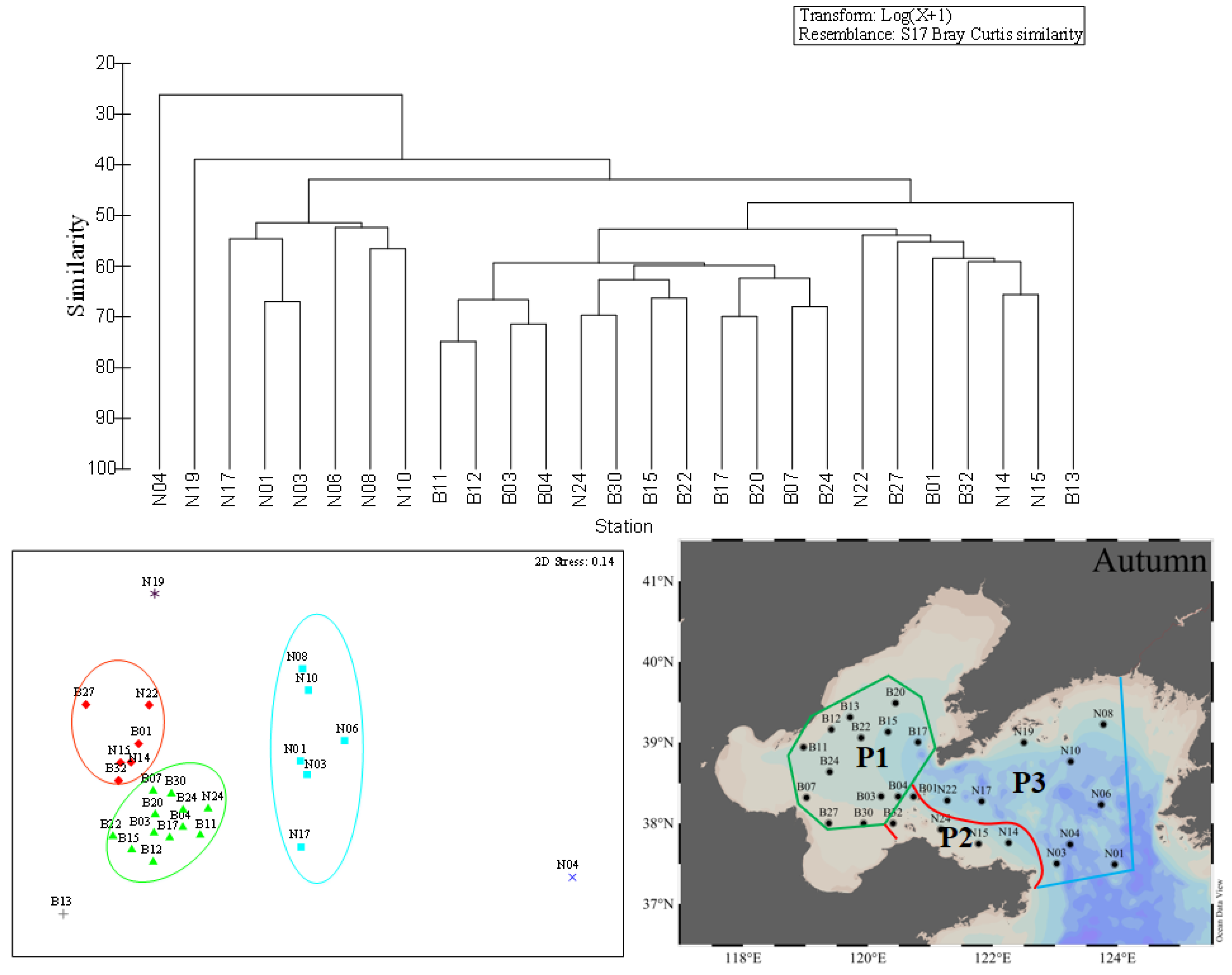
In autumn, the first province consisted of 12 stations, covering all stations in the BS and one station in the NYS just as shown in Figure 7. The mean values of temperature and salinity were 18.7 ± 0.6 °C and 31.5 ± 0.5, respectively. The total phytoplankton abundance ranged between 5.71 × 10³ and 6.40 × 10³ cells·L−1, with the mean value of 2.39 × 10³ cells·L−1. The second province was composed of six stations and these stations distributed in the coastal area of the NYS. The mean values of temperature and salinity were 18.8 ± 0.4 °C and 31.3 ± 0.6, respectively. The total phytoplankton abundance ranged between 5.71 × 10³ and 6.40 × 10³ cells·L−1, with an average value of 2.39 × 10³ cells·L−1. The third province had six stations locating in the NYS, as shown in Figure 5. The temperature ranged from 10.1 to 20.8 °C, with an average of 16.7 ± 3.6 °C. The average value of salinity was 31.9 ± 0.2. Diatoms were the most dominant phytoplankton group in these three provinces, and accounted for 97.8%, 97.6%, 94.2% of the total phytoplankton abundance, respectively. P. sulcata and D. bombus were the dominant species in these three provinces. In addition, B13, N4, and N19 could not be divided into any of the three provinces due to the composition of the top 15 species in these stations having an obvious difference.
The phytoplankton community in the BS and NYS were divided into three ecological provinces in each season (Figure 5, Figure 6 and Figure 7) and the phytoplankton abundance and environmental parameters in the different ecological provinces during the three cruises were shown in Table 5. In summary, we defined the first provinces in three seasons as a province based on the distribution (in the BS) and defined it as P1. We defined the second province in three seasons as a province based on the distribution (in the coastal waters of the NYS) and called it P2. The third provinces (in the NYS) in three seasons were defined as a single province and we called it P3.
3.5. Vertical Distribution of Phytoplankton Abundance
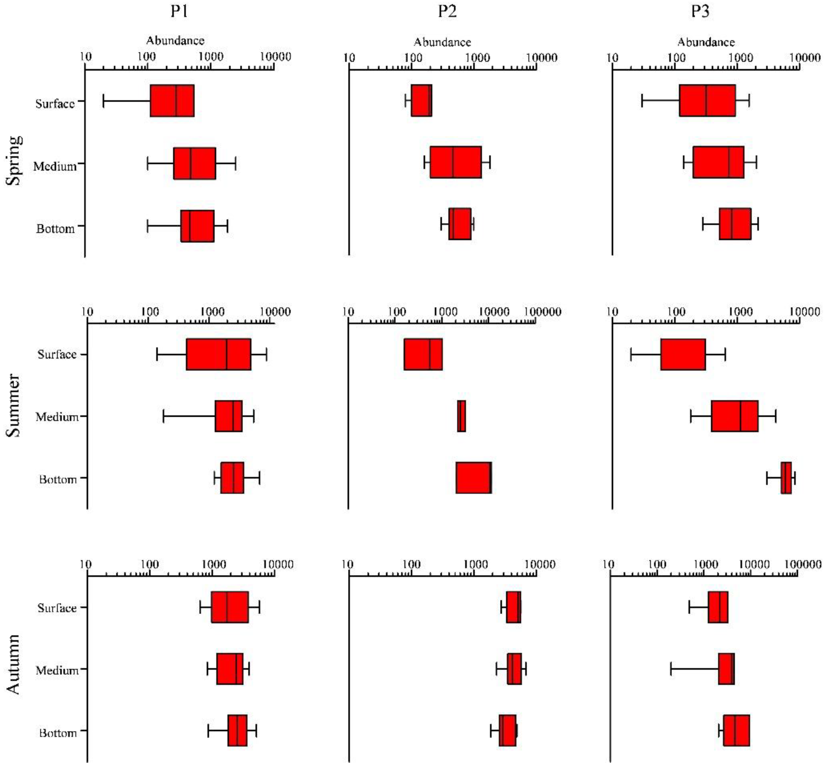
The vertical distribution of total phytoplankton abundance presented an obvious stratification. According to cluster analysis and MDS, we divided the phytoplankton community of the BS and NYS into P1, P2, and P3, and made corresponding box-shaped diagrams (Figure 8). For P1, in spring, the phytoplankton abundance was relatively lower in the surface layer, but the abundance in the middle and the bottom layers was the same and higher compared to the surface layer. In summer, the phytoplankton abundance reached its maximum and the phytoplankton community almost distributed in the surface layer. The phytoplankton abundance in the middle layer was almost the same as that in bottom layer. In autumn, phytoplankton abundance did not differ among surface, middle and bottom layers. For P2, in spring, the phytoplankton abundance was lowest in surface layer and highest in the middle layer. The phytoplankton abundance in the bottom layer was lower than in the middle layer but higher than in the surface layer. In summer, the total phytoplankton abundance increased with depth. In autumn, the phytoplankton were mainly distributed in the surface and middle layers, and the phytoplankton abundance in the bottom layer was relatively low. For P3, in spring, the phytoplankton abundance increased gradually from surface layer to bottom layer. In summer, the phytoplankton abundance gradually increased with depth and was highest in the bottom layer. Additionally, P. sulcata was the dominant specie in the bottom. In autumn, the phytoplankton abundance was same in the surface, middle, and bottom layers.
3.6. Phytoplankton Abundance in Relation to Environment
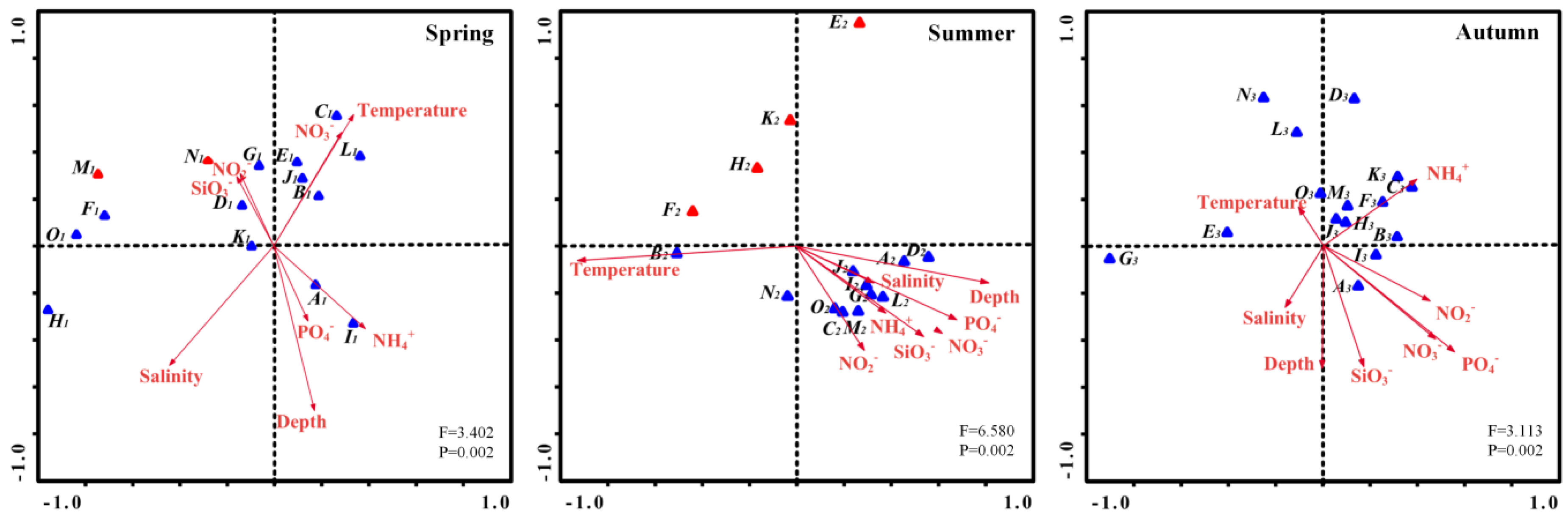
In order to study the association between environmental parameters and phytoplankton community composition, we did a Canonical Correspondence Analysis (CCA) based on the top 15 dominant species in each season and eight environmental variables (temperature, salinity, depth, nitrate, nitrite, phosphate, ammonia, and silicate). The ordination diagram of CCA exhibits phytoplankton community and environmental variables (arrows) during summer, spring and autumn in the BS and NYS (Figure 9). Nutrients, depth, temperature, and salinity were the main variables associated with variation in phytoplankton community.
In spring, the abundances of most dominant diatom species were positively correlated with temperature, silicate, nitrate and nitrite concentrations (Figure 9), while was negatively correlated with depth. However, the abundance of the diatom Guinardia delicatula was not correlate with any environmental parameters. Dinoflagellates showed positive correlations with temperature and nitrite concentrations. In summer, the abundance of D. fibula had a strong positive correlation with temperature. Among the 15 dominant species, all diatoms were positively correlated with salinity, depth, and nutrient concentrations and most dinoflagellates correlated positively with the temperature. In autumn, the majority of diatoms showed positive correlations with temperature, depth, and ammonia concentration, whereas a few showed positively correlated with nitrate, nitrite, and phosphate concentrations.
4. Discussion
4.1. Phytoplankton Community in Different Seasons
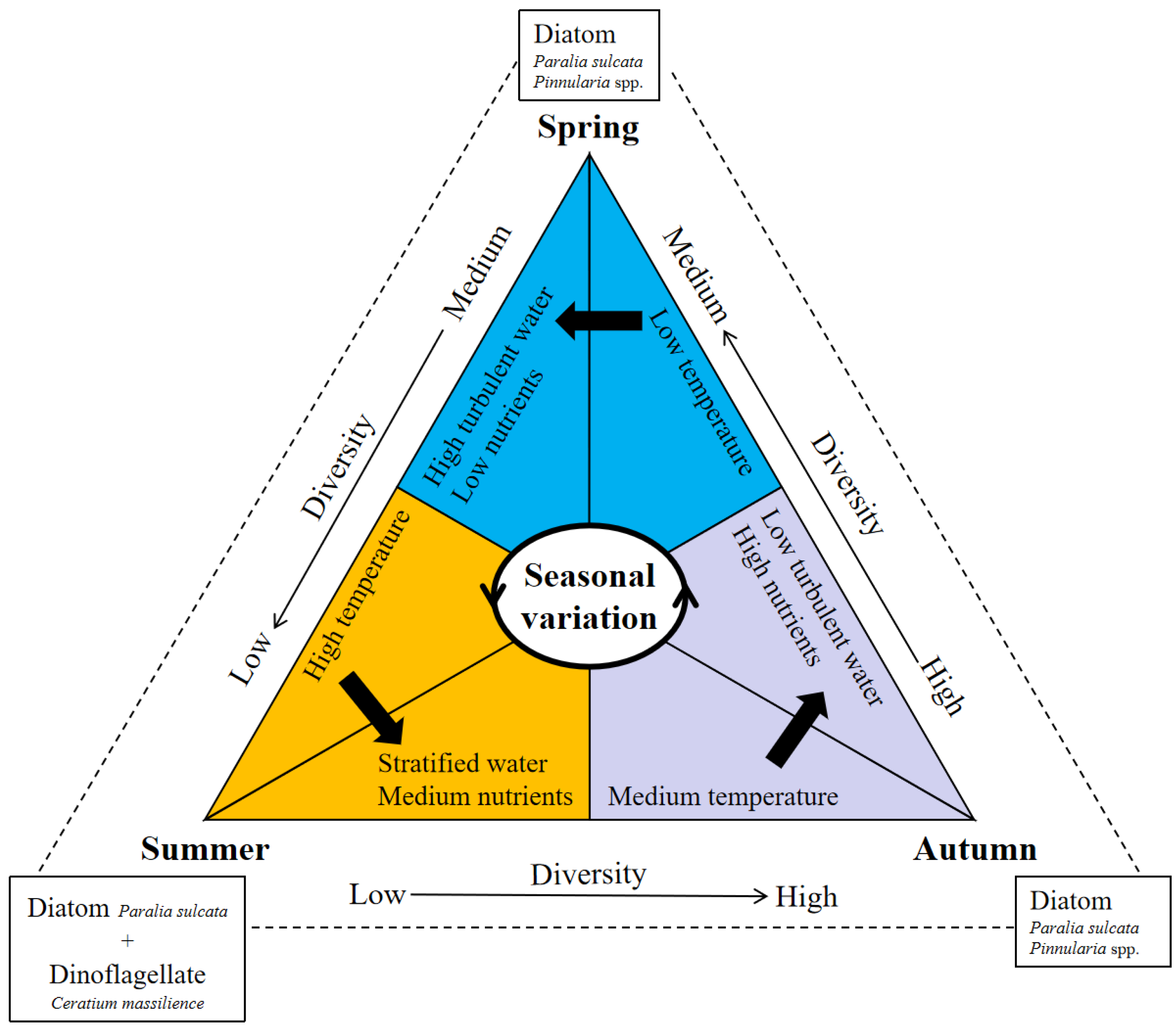
Phytoplankton communities in the BS and NYS are mainly dominated by diatoms, dinoflagellates, and chrysophytas, with diatoms dominating throughout the three seasons and dinoflagellates only dominating in spring and summer (Table 2). In addition, dinoflagellates show a lower occurrence frequency in spring than in summer and autumn. This finding is consistent with previous studies [36,37,38] that diatoms are the dominant phytoplankton group in almost all sampling stations, especially in spring and autumn. Several studies have shown that the combined effects of several environment parameters including nutrients, salinity, temperature, and depth, control the abundance and composition of the phytoplankton in different seasons (Figure 9) [39,40,41]. A simple scenario for seasonal succession patterns of the phytoplankton community in the BS and NYS is proposed here (Figure 10). Research data have revealed that nutrients show a strong seasonal variation due to the differences of terrestrial inputs, phytoplankton uptake, turbulent mixing, transformation and release from organic matter decomposition in BS in different seasons [42]. In spring, seawater mixes evenly due to the low temperature throughout the research area. Besides, the low nutrient concentrations especially the N-compounds caused by uptake are not suitable for the growth and reproduction of all kinds of algae, thus the species diversity is low (Table 4). The temperature rises in the summer and the seawater stratification become obvious, causing growth and reproduction of dinoflagellates. Although the overall cell abundance of phytoplankton increases, the diversity of the community does not increase, and is lower than that in spring (Table 4). In autumn, the concentrations of nutrients increase owing to the disturbance and organic matter decomposition and the temperature begins to decrease [42]. High nutrient levels and a suitable temperature allowed diatoms to grow and reproduce, and the diversity of the community increased significantly. In conclusion, the nutrients levels in different degrees of stratified seawater caused by different temperature in different seasons are the main controlling factor for the phytoplankton communities in the BS and NYS.
According to our CCA analysis, the abundance of dominant diatoms correlates positively with nutrient concentrations and temperature. This indicates that low nutrient level is a significant limiting factor for the growth of diatoms in spring (Figure 9). Concurrently, with yearly increases of nutrients and temperature, the annual bloom of diatoms frequently occurs in the spring. When phosphate is deficient and nitrate is sufficient, the dominants of phytoplankton community will change from diatoms to dinoflagellates [43]. The half-saturation coefficient Ks of phytoplankton species for nutrients is usually used as an indicator for nutrient affinity, and the higher the Ks is, the lower the affinity is [44]. We found a Ks of 1.96 µmol·L−1, which has been reported for P. minimum [44]. In the spring and summer, the average DIP concentration in the BS and NYS is much lower than the Ks of Prorocentrum species (Table 6). In order to adapt to low phosphate concentrations, dinoflagellates such as P. minimum may utilize dissolved organic phosphate (DOP) to survive. Some previous studies have shown that dinoflagellates have the polyculture capabilities including the direct engulfment of prey, pallium feeding, and peduncle feeding [44]. Andersen indicated [45] that the addition of an external nutrient supply, high in N and P but low in Si, influenced algal community structure and function. Yin et al. [46] reported a phenomenon that phosphorus limitation favored the dominance of dinoflagellates in the Pearl River estuary. Stoecker [47] found that phosphorus limitation was a common factor that stimulated the uptake of particulate nutrients by dinoflagellates in field experiments, which might be another reason for the dominance of dinoflagellates in phosphorus- limited conditions. From these viewpoints, we conclude that the phosphate concentration is the significant limiting factor for diatoms and dinoflagellates growth. When the phosphate concentration is less than 0.2 µmol·L−1, it is close to the ecological threshold essential for diatoms growth [48,49]. The phosphate concentration is deficient in the BS and NYS in the spring and summer (Table 5). Therefore, phosphate tends to be the control factor for the surface distribution of diatoms and dinoflagellates abundance in spring and summer.
4.2. Environmental Parameters in Three Provinces
The phosphate concentration is lower in the BS and NYS during the spring (Table 6). Thus, this is the key limitation factor for phytoplankton growth. The levels of DIN (nitrate + ammonia) and DSi in the BS are much higher than those in NYS in three seasons, because the enhanced Yellow River diluted water brings more nutrients to the BS. The DSi level in coastal area is lower than that in the NYS, which is apparently caused by the consumption by phytoplankton blooms and Kuroshio intrusion. Justić et al. [50] have demonstrated that DSi at coastal areas decreases rapidly after diatom blooms in spring. Thereafter, the heterotrophic dinoflagellates increase after the peak of diatom blooms with maximum growth rates [51]. Thus, the diatom abundance in P2 is lower than in P3 during spring. The number of dinoflagellates increases quickly in summer (Table 5). Additionally, the DIP exhibits high levels around NYS in autumn. Consequently, a high phytoplankton abundance occurs in P2 (with the mean value of 4.12 × 10³ cells·L−1) and P3 (with the mean value of 5.85 × 10³ cells·L−1). Furthermore, according to the CCA, the majority of diatoms have negative correlations with the depth, thus, depth plays an important role in controlling algal density. Compared to P2 and P3, the phytoplankton abundance in P1 is relatively low despite of high nutrient levels in autumn. Overall, our study confirms that the distribution of ecological assemblages is mainly related to the physicochemical properties (for example: nutrients, depth, and temperature).
Phytoplankton in the BS and NYS has changing compositions and distributions across the seasons (Figure 11). More details should be considered based on different water types when studying phytoplankton in the BS and NYS. Additionally, P1 represents most parts of the BS and is influenced by the BSMW and BSSCW in spring [52]. The phosphate and nitrate concentrations increase significantly (Table 6), due to the sediment resuspension and organic matter decomposition in autumn [16]. Accordingly, the low abundance of phytoplankton in P1 in spring is likely caused by inhibiting effects of nutrient limitation. Jiang et al. [12] have proposed that the Yellow Sea is mainly controlled by the YSWC, YSCWM and coastal run-off. The YSCWM begins to form in spring every year, and reaches its peak in summer, and then gradually weakens in autumn, and disappears entirely in winter [53]. P3 is characterized by low-temperature and high-salinity and is located in NYS. It is primarily controlled by the YSCWM. In autumn, the internal concentration of nutrient is at a high level and the phytoplankton abundance reaches its maximum. The dominant species are diatoms, which agrees with previous field investigation [54]. The YSCWM has a significant influence on the temporal and spatial distribution of the phytoplankton community structures during its development, prevalence and decline: in the prevailing period, the temperature is low, and the salinity is high (Figure 2), and the structure of the phytoplankton community also presents the obvious vertical discrepancy (Figure 8). Generally, we confirm that the various composition and vertical discrepancy of phytoplankton in three ecological provinces are mainly affected by the physicochemical properties caused by water masses and circulations.
Author Contributions
J.S. designed this study. Y.W., Z.L., Y.X., Y.G. and T.G. performed the experiments and analysis. X.F. wrote the manuscript and prepared the tables and figures. All authors edited the manuscript. All authors have read and agreed to the published version of the manuscript.
Funding
This study was financially supported by the National Key Research and Development Project of China (2019YFC1407805), the National Natural Science Foundation of China (41876134, 41676112 and 41276124), the Tianjin 131 Innovation Team Program (20180314), and the Changjiang Scholar Program of Chinese Ministry of Education (T2014253) to J.S. CTD Data and water samples were collected onboard of R/V “Beidou” implementing the open research cruise NORC2019-01 supported by NSFC Shiptime Sharing Project (project number: 41849901).
Institutional Review Board Statement
Not applicable.
Informed Consent Statement
Not applicable.
Data Availability Statement
Not applicable.
Conflicts of Interest
The authors declare no conflict of interest.
References
- Barton, A.D.; Lozier, M.S.; Williams, R.G. Physical controls of variability in North Atlantic phytoplankton communities. Limnol. Oceanogr. 2015, 60, 181–197. [Google Scholar] [CrossRef] [Green Version]
- Field, C.B.; Behrenfeld, M.J.; Randerson, J.T.; Falkowski, P.G. Primary production of the biosphere: Integrating terrestrial and oceanic components. Science 1998, 281, 237–240. [Google Scholar] [CrossRef] [Green Version]
- Falkowski, P.G.; Barber, R.T.; Smetacek, V. Biogeochemical controls and feedbacks onocean primary production. Science 1998, 281, 200–206. [Google Scholar] [CrossRef] [PubMed] [Green Version]
- Boyce, D.G.; Lewis, M.R.; Worm, B. Global phytoplankton decline over the past century. Nature 2010, 466, 591–596. [Google Scholar] [CrossRef] [PubMed]
- Paerl, H.W.; Rossignol, K.L.; Hall, S.N.; Peierls, B.L.; Wetz, M.S. Phytoplankton community indicators of short- and long-term ecological change in the anthropogenically and climatically impacted Neuse River Estuary, North Carolina, USA. Estuar. Coast. 2010, 33, 485–497. [Google Scholar] [CrossRef]
- Guo, S.; Feng, Y.; Wang, L.; Dai, M.; Liu, Z.; Bai, Y.; Sun, J. Seasonal variation in the phytoplankton community of a continental-shelf sea: The East China Sea. Mar. Ecol. Prog. Ser. 2014, 516, 103–126. [Google Scholar] [CrossRef] [Green Version]
- Platt, T.; Sathyendranath, S. Spatial structure of pelagic ecosystem processes in the global ocean. Ecosystems 1999, 2, 384–394. [Google Scholar] [CrossRef]
- Devred, E.; Sathyendranath, S.; Platt, T. Delineation of ecological provinces using ocean colour radiometry. Mar. Ecol. Prog. Ser. 2007, 346, 1–13. [Google Scholar] [CrossRef]
- Longhurst, A.R. Ecological Geography of the Sea; Academic Press: London, UK, 1998; pp. 1–527. [Google Scholar]
- Longhurst, A.; Sathyendranath, S.; Platt, T.; Caverhill, C. An estimate of global primary production in the ocean from satellite radiometer data. J. Plankton Res. 1995, 17, 1245–1271. [Google Scholar] [CrossRef] [Green Version]
- Taylor, B.B.; Torrecilla, E.; Bernhardt, A.; Taylor, M.H.; Peeken, I.; Rottgers, R.; Piera, J.; Bracher, A. Biooptical provinces in the eastern Atlantic Ocean and their biogeographical relevance. Biogeosciences 2011, 8, 7165–7219. [Google Scholar] [CrossRef] [Green Version]
- Jiang, Z.; Chen, J.; Zhou, F.; Shou, L.; Chen, Q.; Tao, B.; Wang, K. Controlling factors of summer phytoplankton community in the Changjiang (Yangtze River) Estuary and adjacent East China Sea shelf. Cont. Shelf Res. 2015, 101, 71–84. [Google Scholar] [CrossRef]
- Su, Y.S.; Weng, X.C. Water masses in China seas. In Oceanology of China Seas; Springer: Dordrecht, The Netherlands, 1994; pp. 3–16. [Google Scholar] [CrossRef]
- Shi, Q. Spatio-temporal modes and circulation variation on the interannual variation of seasonal mean wind-driven current field in the Bohai Sea and Yellow Sea in winter and summer. J. Appl. Oceanogr. 2019, 38, 93–108. (In Chinese) [Google Scholar]
- Naimie, C.E.; Blain, C.A.; Lynch, D.R. Seasonal mean circulation in the Yellow Sea—a model-generated climatology. Cont. Shelf Res. 2001, 21, 667–695. [Google Scholar] [CrossRef]
- Luan, Q.S.; Kang, Y.D.; Wang, J. Long-term changes on phytoplankton community in the Bohai Sea (1959~2015). Prog. Fish. Sci. 2018, 39, 09–18. (In Chinese) [Google Scholar] [CrossRef]
- Lin, C.; Ning, X.; Su, J.; Lin, Y.; Xu, B. Environmental changes and the responses of the ecosystems of the Yellow Sea during 1976–2000. J. Mar. Syst. 2004, 55, 223–234. [Google Scholar] [CrossRef]
- Sun, J.; Liu, D.Y. The preliminary notion on nomenclature of common phytoplankton in China Seas waters. Oceanol. Limnol. Sin. 2002, 03, 271–286. (In Chinese) [Google Scholar] [CrossRef]
- Sun, J.; Liu, D.Y.; Yang, S.M.; Guo, J.; Qian, S.B. The Preliminary Study on Phytoplankton Community Structure in the Central Bohai Sea and the Bohai Strait and Its Adjacent Area. Oceanol. Limnol. 2002, 5, 461–471. (In Chinese) [Google Scholar] [CrossRef]
- Jin, J.; Liu, S.M.; Ren, J.L.; Liu, C.G.; Zhang, J.; Zhang, G.L.; Huang, D.J. Nutrient dynamics and coupling with phytoplankton species composition during the spring blooms in the Yellow Sea. Deep. Sea Res. Part. II Top. Stud. Oceanogr. 2013, 97, 16–32. [Google Scholar] [CrossRef]
- Liu, H.J.; Huang, Y.J.; Zhai, W.D.; Jin, H.; Sun, J. Phytoplankton communities and its controlling factors in summer and autumn in the southern Yellow Sea, China. Acta Oceanol. Sin. 2015, 34, 114–123. (In Chinese) [Google Scholar] [CrossRef]
- Liu, X.; Chiang, K.P.; Liu, S.M.; Wei, H.; Zhao, Y.; Huang, B.Q. Influence of the Yellow Sea Warm Current on phytoplankton community in the central Yellow Sea. Deep Sea Res. Part I Oceanogr. Res. Pap. 2015, 106, 17–29. [Google Scholar] [CrossRef]
- Zhang, P.R.Y.; Li, D.L.; Dai, Y.Y.; Gao, Y.; Zhang, J.W.; Yang, W.Y.; Liu, K.F.; Liu, X.B. The characteristic of phytoplankton community structure in the coastal area of Tianjin. Trans. Oceanol. Limnol. 2016, 53–59. (In Chinese) [Google Scholar] [CrossRef]
- Utermöhl, V.H. Neue Wege in der quantitativen Erfassung des Planktons. (Mit besonderer Berücksichtigung des Ultraplanktons.). SIL Proc. 1931, 5, 567–596. [Google Scholar] [CrossRef]
- Dexiang, J. Chinese Marine Planktonic Diatoms; Shanghai Scientific and Technical Publishers: Shanghai, China, 1965. (In Chinese) [Google Scholar]
- Yamaji, I. Illustrations of the Marine Plankton of Japan; Hoikusha Publishing Co. Ltd.: Osaka, Japan, 1966; pp. 1–538. (In Japanese) [Google Scholar]
- Liu, S.M.; Li, R.H.; Zhang, G.L.; Wang, D.R.; Du, J.Z.; Herbeck, L.S.; Zhang, J.; Ren, J.L. The impact of anthropogenic activities on nutrient dynamics in the tropical Wenchanghe and Wenjiaohe Estuary and Lagoon system in East Hainan, China. Mar. Chem. 2005, 125, 49–68. [Google Scholar] [CrossRef]
- Shannon, C.E. A mathematical theory of communication. Bell Syst. Tech. J. 1951, 27, 379–423. [Google Scholar] [CrossRef] [Green Version]
- Sun, J.; Liu, D.Y. The application of diversity indices in marine phytoplankton studies. Acta Oceanol. Sin. 2004, 26, 62–75. (In Chinese) [Google Scholar] [CrossRef]
- Hall, H.B. The Interpretation of Ecological Data: A primer on classification and ordination. For. Ecol. Manag. 1984, 1–230. [Google Scholar] [CrossRef]
- Sun, J.; Liu, D.Y.; Ning, X.R.; Liu, C.G. Phytoplankton in the Prydz Bay and the adjacent Indian sector of the Southern Ocean during the austral summer 2001/2002. Oceanol. Limnol. Sin. 2003, 34, 519–532. (In Chinese) [Google Scholar] [CrossRef]
- Jaccard, P. Nouvelles recherches surla distribution florale. Bulletin de la Société Vaudense des Sciences Naturelles 1908, 44, 223–270. [Google Scholar] [CrossRef]
- Zhu, J.; Zheng, Q.N.; Hu, J.Y.; Lin, H.Y.; Chen, D.W.; Chen, Z.Z.; Sun, Z.Y.; Li, L.Y.; Kong, H. Classification and 3-D distribution of upper layer water masses in the northern South China Sea. Acta Oceanol. Sin. 2019, 38, 126–135. [Google Scholar] [CrossRef]
- Clarke, K.R.; Gorley, R.N. PRIMER v5: User Manual/Tutorial; Primer-E Limited: Auckland, New Zealand, 2001. [Google Scholar]
- Sun, J.; Gu, X.Y.; Feng, Y.Y.; Jin, S.F.; Jiang, W.S.; Jin, H.Y.; Chen, J.F. Summer and winter living coccolithophores in the Yellow Sea and the East China Sea. Biogeosciences 2014, 11, 779–806. [Google Scholar] [CrossRef] [Green Version]
- Sun, J.; Liu, D.Y.; Wang, W.; Chen, K.B.; Qin, Y.T. The netz-phytoplankton community of the central Bohai Sea and its adjacent waters in autumn, 1998. Acta Ecol. Sin. 2004, 24, 1643–1655. (In Chinese) [Google Scholar] [CrossRef]
- Sun, J.; Liu, D.Y. Net phytoplankton community of the Bohai Sea in the autumn of 2000. Acta Pharmacol. Sin. 2005, 27, 124–132. (In Chinese) [Google Scholar] [CrossRef]
- Li, X.Q.; Feng, Y.Y.; Leng, X.Y.; Liu, H.J.; Sun, J. Phytoplankton Species Composition of Four Ecological Provinces in Yellow Sea, China. J. Ocean Univ. China 2017, 16, 1115–1125. (In Chinese) [Google Scholar] [CrossRef]
- Struyf, E.; Smis, A.; Damme, S.V.; Meire, P.; Conley, D.J. The global biogeochemical silicon cycle. Silicon 2009, 1, 207–213. [Google Scholar] [CrossRef]
- Koçum, E. Autotrophic nanoplankton dynamics is significant on the spatio-temporal variation of phytoplankton biomass size structure along a coastal trophic gradient. Reg. Stud. Mar. Sci. 2020, 33, 100920. [Google Scholar] [CrossRef]
- Luan, Q.S.; Sun, J.; Shen, Z.L.; Song, S.Q.; Wang, M. Phytoplankton assemblage of Yangtze River Estuary and the adjacent East China Sea in summer, 2004. J. Ocean Univ. China 2006, 2, 123–131. (In Chinese) [Google Scholar] [CrossRef]
- Zhang, H.B.; Liu, K.; Wang, L.S.; Shi, X.Y.; Feng, L.N.; Wang, X. Seasonal variation of nutrients forms and its effects on nutrients pools in the center of the Bohai Sea, China. Acta Ecol. Sin. 2020, 40, 5424–5432. (In Chinese) [Google Scholar] [CrossRef]
- Richardson, K. Harmful or exceptional phytoplankton blooms in the marine ecosystem. Adv. Mar. Biol. 1997, 31, 301–385. [Google Scholar] [CrossRef]
- Smayda, T.J. Harmful algal blooms: Their ecophysiology and general relevance to phytoplankton blooms in the sea. Limnol. Oceanogr. 1997, 42, 1137–1153. [Google Scholar] [CrossRef]
- Andersen, I.M.; Williamson, T.J.; González, M.J.; Vanni, M.J. Nitrate, ammonium, and phosphorus drive seasonal nutrient limitation of chlorophytes, cyanobacteria, and diatoms in a hyper-eutrophic reservoir. Limnol. Oceanogr. 2020, 65, 962–978. [Google Scholar] [CrossRef]
- Yin, K.; Qian, P.Y.; Chen, J.C.; Hsieh, D.P.H.; Harrison, P.J. Dynamics of nutrients and phytoplankton biomass in the Pearl River estuary and adjacent waters of Hong Kong during summer: Preliminary evidence for phosphorus and silicon limitation. Mar. Ecol. Prog. Ser. 2000, 194, 295–305. [Google Scholar] [CrossRef]
- Stoecker, D.K. Mixotrophy among dinoflagellates. J. Eukaryot. Microbiol. 1999, 46, 397–401. [Google Scholar] [CrossRef]
- Zou, J.; Dong, L.; Qin, B. Preliminary analyze of seawater wealthy nutrients and red tide in the Bohai Sea. Hydrobiologia 1983, 2, 42–54. [Google Scholar] [CrossRef]
- Wang, Y.M.; Ding, J.X.; Zhang, J. Analysis of characteristics of evolution on the ecological environment and impact factors in Bohai Sea. J. Ludong Univ. Nat. Sci. Ed. 2016, 32, 66–73. (In Chinese) [Google Scholar]
- Justić, D.; Rabalais, N.N.; Turner, R.E.; Dortch, Q. Changes in nutrient structure of river-dominated coastal waters: Stoichiometric nutrient balance and its consequences. Estuar. Coast. Shelf Sci. 1995, 40, 339–356. [Google Scholar] [CrossRef]
- Tiselius, P.; Kuylenstierna, B. Growth and decline of a diatom spring bloom phytoplankton species composition, formation of marine snow and the role of heterotrophic dinoflagellates. J. Plankton Res. 1996, 18, 133–155. [Google Scholar] [CrossRef]
- Wei, Y.Q.; Liu, H.J.; Zhang, X.D.; Munir, S.; Sun, J. Physicochemical conditions in affecting the distribution of spring phytoplankton community. Chin. J. Oceanol. Limnol. 2017, 35, 1342–1361. (In Chinese) [Google Scholar] [CrossRef]
- Su, J.L.; Wang, D.J. On the current field associated with the Yellow Sea Cold Water Mass. Oceanol. Limnol. Sin. Suppl. 1995, 1–7. (In Chinese) [Google Scholar] [CrossRef]
- Yuan, M.L.; Sun, J.; Zhai, W.D. Phytoplankton Community in Bohai Sea and the North Yellow Sea in Autumn 2012. J. Tianjin Univ. Sci. Technol. 2014, 29, 56–64. (In Chinese) [Google Scholar] [CrossRef]
Figure 1.
Location of sampling stations (black dots) during three cruises in the BS and NYS. The name of the stations is defined as “Bn” at BS and “Nn” at NYS and the color bar is bathymetry.
Figure 1.
Location of sampling stations (black dots) during three cruises in the BS and NYS. The name of the stations is defined as “Bn” at BS and “Nn” at NYS and the color bar is bathymetry.

Figure 2.
Temperature-salinity (T-S) relationship of sea water during three cruises (spring, summer, autumn) in the BS and NYS. A salinity of ~31 psu characterizes the coastal water system (dashed blue line), and x-axis is salinity, y-axis is temperature, and the isobars are density. NYS is the north Yellow Sea and BS is the Bohai Sea.

Figure 3.
Pie charts of the top 15 dominant phytoplankton taxa in different seasons based on water column integration. The pie chart size is related to cell density as shown in Figure 3.
Figure 3.
Pie charts of the top 15 dominant phytoplankton taxa in different seasons based on water column integration. The pie chart size is related to cell density as shown in Figure 3.

Figure 4.
Sea surface distribution of phytoplankton, Bacillariophyta, Pyrrhophyta, and Chrysophyta (cells·L−1) in different seasons. The color bar is cell abundance.
Figure 4.
Sea surface distribution of phytoplankton, Bacillariophyta, Pyrrhophyta, and Chrysophyta (cells·L−1) in different seasons. The color bar is cell abundance.


Figure 5.
Cluster analysis (left) and MDS (right) of the top 15 dominant species at each sampling station in spring. Each symbol represents a sampling station: green triangles = first assemblage, blue squares = second assemblage; red diamonds = third assemblage.
Figure 5.
Cluster analysis (left) and MDS (right) of the top 15 dominant species at each sampling station in spring. Each symbol represents a sampling station: green triangles = first assemblage, blue squares = second assemblage; red diamonds = third assemblage.

Figure 6.
Cluster analysis (left) and MDS (right) of the top 15 dominant species at each station in summer. Each symbol represents a sampling station: green triangles = fourth assemblage; blue squares = fifth assemblage; red diamonds = sixth assemblage.
Figure 6.
Cluster analysis (left) and MDS (right) of the top 15 dominant species at each station in summer. Each symbol represents a sampling station: green triangles = fourth assemblage; blue squares = fifth assemblage; red diamonds = sixth assemblage.

Figure 7.
Cluster analysis (left) and MDS (right) of the top 15 dominant species with station in autumn. Each symbol represents a sampling station: green triangles = fourth assemblage; blue squares = fifth assemblage; red diamonds = sixth assemblage.
Figure 7.
Cluster analysis (left) and MDS (right) of the top 15 dominant species with station in autumn. Each symbol represents a sampling station: green triangles = fourth assemblage; blue squares = fifth assemblage; red diamonds = sixth assemblage.

Figure 8.
Box-Whisker plots of phytoplankton cell abundance (cells·L−1) in the BS and NYS in the three seasons. Whiskers mean minimum and maximum values; boxes display the lower and upper quartiles; and lines mean median sets. P1, P2 and P3 are the provinces grouped.
Figure 8.
Box-Whisker plots of phytoplankton cell abundance (cells·L−1) in the BS and NYS in the three seasons. Whiskers mean minimum and maximum values; boxes display the lower and upper quartiles; and lines mean median sets. P1, P2 and P3 are the provinces grouped.

Figure 9.
Ordination diagram of canonical correspondence analysis (CCA) exhibits phytoplankton community and environmental variables (arrows) during summer, spring, and autumn in the BS and NYS. A-O indicates the top 15 dominant species in each season listed in Table 2, the red triangles are Pyrrophyta and the blue triangles are Bacillariophyta.

Figure 10.
Schematic of seasonal succession of the phytoplankton community in the BS and NYS.

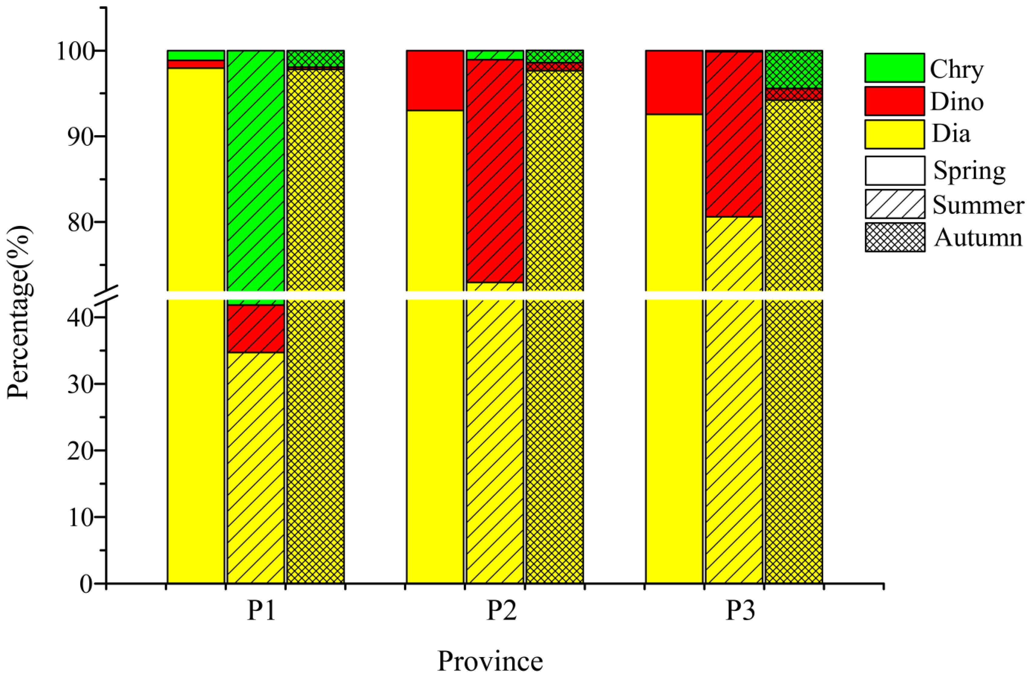
Figure 11.
Seasonal percentage of different phytoplankton taxa in different seasons.


Table 1.
The depth (m) of the water samples in the Bohai Sea (BS) and the North Yellow Sea (NYS) in three seasons.
Table 1.
The depth (m) of the water samples in the Bohai Sea (BS) and the North Yellow Sea (NYS) in three seasons.
| Spring | Summer | Autumn | |||||||||
|---|---|---|---|---|---|---|---|---|---|---|---|
| Station | Surface | Middle | Bottom | Station | Surface | Middle | Bottom | Station | Surface | Middle | Bottom |
| B01 | 4 | 13 | 24 | B01 | 3 | 12 | 25 | B01 | 4 | 14 | 24 |
| B03 | 4 | 13 | 23 | B03 | 3 | 13 | 23 | B03 | 4 | 14 | 24 |
| B04 | 4 | 12 | 21 | B04 | 3 | 13 | 23 | B04 | 4 | 13 | 23 |
| B07 | 4 | 8 | 14 | B07 | 3 | 10 | 16 | B07 | 4 | 10 | 17 |
| B09 | 4 | 11 | 20 | B09 | 3 | 12 | 21 | B11 | 4 | 11 | 19 |
| B10 | 4 | 13 | 23 | B11 | 3 | 10 | 18 | B12 | 4 | 11 | 19 |
| B11 | 4 | 10 | 18 | B12 | 3 | 10 | 18 | B13 | 4 | 13 | 22 |
| B12 | 4 | 10 | 17 | B13 | 3 | 12 | 22 | B15 | 4 | 11 | 18 |
| B13 | 4 | 11 | 20 | B15 | 3 | 11 | 19 | B17 | 4 | 18 | 32 |
| B17 | 4 | 18 | 33 | B17 | 3 | 17 | 37 | B20 | 4 | 13 | 23 |
| B19 | 4 | 14 | 25 | B20 | 3 | 13 | 23 | B22 | 4 | 12 | 20 |
| B20 | 4 | 12 | 21 | B22 | 3 | 11 | 20 | B24 | 4 | 13 | 23 |
| B22 | 4 | 11 | 13 | B24 | 3 | 13 | 23 | B27 | 4 | 9 | 15 |
| B24 | 4 | 11 | 21 | B27 | 3 | 8 | 13 | B30 | 4 | 9 | 16 |
| B25 | 4 | 11 | 19 | B30 | 3 | 8 | 15 | B32 | 4 | 9 | 15 |
| B26 | 4 | 6 | 9 | B31 | 3 | 8 | 14 | N01 | 4 | 34 | 64 |
| B27 | 4 | 7 | 13 | B32 | 3 | 8 | 15 | N03 | 4 | 26 | 48 |
| B31 | 4 | 8 | 14 | N01 | 3 | 30 | 61 | N04 | 4 | 33 | 63 |
| B32 | 4 | 8 | 14 | N03 | 3 | 20 | 64 | N06 | 4 | 32 | 61 |
| N01 | 4 | 15 | 63 | N04 | 3 | 20 | 65 | N08 | 4 | 22 | 40 |
| N03 | 4 | 22 | 42 | N06 | 3 | 20 | 65 | N10 | 4 | 28 | 51 |
| N04 | 4 | 15 | 63 | N08 | 3 | 20 | 35 | N14 | 4 | 13 | 23 |
| N06 | 4 | 15 | 63 | N10 | 3 | 15 | 48 | N15 | 4 | 11 | 17 |
| N08 | 4 | 18 | 34 | N12 | 3 | 18 | 50 | N17 | 4 | 27 | 50 |
| N10 | 4 | 15 | 53 | N14 | 3 | 10 | 22 | N19 | 4 | 19 | 35 |
| N12 | 4 | 15 | 52 | N15 | 3 | 7 | 17 | N22 | 4 | 25 | 40 |
| N14 | 4 | 13 | 24 | N17 | 3 | 18 | 36 | N24 | 4 | 11 | 18 |
| N15 | 4 | 11 | 18 | N19 | 3 | 13 | 36 | ||||
| N17 | 4 | 15 | 47 | N20 | 3 | 18 | 46 | ||||
| N19 | 4 | 19 | 36 | N22 | 3 | 18 | 39 | ||||
| N20 | 4 | 15 | 47 | N23 | 3 | 15 | 28 | ||||
| N21 | 4 | 15 | 50 | N24 | 3 | 15 | 17 | ||||
| N22 | 4 | 18 | 42 | ||||||||
| N24 | 4 | 9 | 15 | ||||||||
Table 2.
Top 15 dominant phytoplankton species during three seasons (spring, summer, and autumn) in the BS and NYS. The alphabetical order in the left column is the order of dominance from largest to smallest.
Table 2.
Top 15 dominant phytoplankton species during three seasons (spring, summer, and autumn) in the BS and NYS. The alphabetical order in the left column is the order of dominance from largest to smallest.
| Spring | Summer | Autumn |
|---|---|---|
| A Paralia sulcata b | Paralia sulcatab | Paralia sulcatab |
| B Pinnularia spp. b | Dictyocha fibulac | Diploneis bombusb |
| C Pleurosigma spp. b | Diploneis bombusb | Nitzschia spp. b |
| D Thalassiosira spp. b | Thalassiosira eccentricab | Pseudonitzschia delicatissimab |
| E Coscinodiscus granii b | Tripos massiliensis f. armatus a | Dictyocha fibulac |
| F Thalassiosira nordenskioeldii b | Gyrodinium spiralea | Pleurosigma spp. b |
| G Coscinodiscus spp. b | Coscinodiscus graniib | Rhizosolenia similisb |
| H Guinardia delicatula b | Prorocentrum minimuma | Thalassiosira spp. b |
| I Thalassiosira eccentrica b | Coscinodiscus spp. b | Coscinodiscus spp. b |
| J Coscinodiscus subtilis b | Pinnularia spp. b | Coscinodiscus graniib |
| K Nitzschia spp. b | Tripos longipesa | Coscinodiscus subtilisb |
| L Navicula spp. b | Coscinodiscus subtilisb | Meuniera membranaceab |
| M Scrippsiella troichoidea a | Pleurosigma spp. b | Navicula spp. b |
| N Prorocentrum minimum a | Nitzschia spp. b | Nitzschia lorenzianab |
| O Thalassiosira rotula b | Coscinodiscus curvatulusb | Pinnularia spp. b |
a Dinoflagellate; b diatom; c chrysophyta.
Table 3.
The Jaccard similarity index of phytoplankton community in three seasons (spring, summer, and autumn) in the BS and NYS. The number of identified species is the number of phytoplankton species we have identified in each season.
Table 3.
The Jaccard similarity index of phytoplankton community in three seasons (spring, summer, and autumn) in the BS and NYS. The number of identified species is the number of phytoplankton species we have identified in each season.
| Seasons | Spring/Summer | Summer/Autumn | Spring/Autumn |
|---|---|---|---|
| Number of identified species | 44 | 56 | 52 |
| Similarity index value | 0.34 | 0.30 | 0.29 |
Table 4.
The diversity index (H) and evenness index (J) of phytoplankton community in three seasons (spring, summer, and autumn) in the BS and NYS.
Table 4.
The diversity index (H) and evenness index (J) of phytoplankton community in three seasons (spring, summer, and autumn) in the BS and NYS.
| Season | Surface | Medium | Bottom | Average | ||||
|---|---|---|---|---|---|---|---|---|
| H | J | H | J | H | J | H | J | |
| Spring | 1.99 ± 0.55 | 0.78 ± 0.15 | 1.96 ± 0.74 | 0.67 ± 0.23 | 1.93 ± 0.72 | 0.65 ± 0.21 | 1.96 ± 0.67 | 0.70 ± 0.19 |
| Summer | 1.56 ± 0.84 | 0.62 ± 0.28 | 1.68 ± 0.74 | 0.50 ± 0.18 | 1.54 ± 0.65 | 0.43 ± 0.17 | 1.59 ± 0.74 | 0.52 ± 0.21 |
| Autumn | 2.62 ± 0.80 | 0.62 ± 0.17 | 2.62 ± 0.79 | 0.62 ± 0.19 | 2.41 ± 0.87 | 0.57± 0.18 | 2.55 ± 0.82 | 0.60 ± 0.18 |
Table 5.
Phytoplankton abundance (cells·L−1) (means, SD in parentheses) and environmental parameters in the different ecological assemblages during three cruises (spring, summer and fall) in the BS and NYS. (Phyto: phytoplankton, Dino: dinoflagellates, Chry: Chrysophyta, T: temperature, S: salinity).
| Region | Season | Phyto/Cells·L−1 | Diatom/Cells·L−1 | Dino/Cells·L−1 | Chry/Cells·L−1 | T(°C) | S | NO3--N/µmol·L−1 | PO43--P/µmol·L−1 | SiO32−-Si/µmol·L−1 | NH4+/µmol·L−1 | Depth/m |
|---|---|---|---|---|---|---|---|---|---|---|---|---|
| P1 | Spring | 703.3 (864.6) | 695.8 (866.4) | 7.5 (12.1) | 10.2 (25.3) | 10.2 (1.3) | 31.6 (1.0) | 3.1 (2.9) | 0.04 (0.1) | 1.0 (0.66) | 1.1 (0.5) | 10.6 (6.3) |
| Summer | 5270.2 (12,158.7) | 1827.8 (1684.0) | 376.3 (692.5) | 3066.1 (11,973.5) | 22.7 (3.8) | 31.3 (1.1) | 2.0 (1.6) | 0.10 (0.1) | 5.3 (2.0) | 1.6 (0.9) | 11.5 (7.9) | |
| Autumn | 2394.2 (1331.2) | 2341.7 (1307.3) | 6.4 (11.7) | 46.1 (56.5) | 18.7 (0.6) | 31.5 (0.5) | 3.9 (2.7) | 0.40 (0.1) | 4.3 (1.6) | 1.1 (0.4) | 12.1 (7.9) | |
| P2 | Spring | 563.3 (544.9) | 523.9 (571.9) | 39.4 (53.8) | 0 | 8.9 (1.8) | 31.8 (0.1) | 1.3 (1.7) | 0.03 (0.03) | 0.9 (0.5) | 1.5 (0.4) | 14.5 (10.6) |
| Summer | 3760 (4254.1) | 2743.3 (4690.4) | 976.7 (1017.4) | 40 (69.3) | 17.8 (6.1) | 31.6 (0.5) | 1.0 (0.8) | 0.12 (0.1) | 1.7 (0.9) | 1.4 (0.7) | 18.9 (14.8) | |
| Autumn | 4123.9 (1414.2) | 4026.7 (1429.0) | 38.9 (61.3) | 58.3 (52.7) | 18.9 (0.4) | 31.3 (0.6) | 3.7 (3.8) | 0.24 (0.1) | 4.0 (1.3) | 1.4 (0.6) | 13.2 (9.9) | |
| P3 | Spring | 847.7 (765.1) | 784.7 (770.1) | 63 (77.1) | 0 | 8.1 (1.6) | 32.2 (0.1) | 2.2 (0.9) | 0.1 (0.1) | 1.2 (3.4) | 1.1 (0.7) | 24.1 (21.4) |
| Summer | 2590.6 (3165.7) | 2088.3 (3128.0) | 498.9 (988.6) | 3.3 (11.2) | 17.4 (7.3) | 31.9 (0.3) | 1.9 (1.2) | 0.15 (0.1) | 2.4 (1.1) | 1.4 (0.7) | 20.9 (20.3) | |
| Autumn | 5851.7 (6591.9) | 5514.4 (6459.0) | 78.9 (85.1) | 258.3 (355.3) | 16.7 (3.6) | 31.9 (0.2) | 3.2 (3.1) | 0.25 (0.2) | 4.1 (2.0) | 0.9 (0.5) | 28.2 (21.0) |
Table 6.
Range and mean values of nutrient concentrations (µmol·L−1) in three seasons.
| Survey Area | Season | Ammonium | Phosphate | Nitrate | Silicate | |
|---|---|---|---|---|---|---|
| BS | Spring | Range | 0.37–2.22 | 0.003–0.27 | 0.01–14.76 | 0.19–3.38 |
| Mean | 1.17 ± 0.48 | 0.06 ± 0.07 | 3.24 ± 2.92 | 1.09 ± 0.78 | ||
| BS | Summer | Range | 0.60–6.05 | 0.003–0.29 | 0.31–7.93 | 1.63–9.25 |
| Mean | 1.56 ± 0.92 | 0.10 ± 0.09 | 2.01 ± 1.80 | 5.30 ± 2.03 | ||
| BS | Autumn | Range | 0.06–1.74 | 0.22–0.64 | 1.27–14.11 | 1.01–7.35 |
| Mean | 1.05 ± 0.45 | 0.38 ± 0.11 | 4.24 ± 2.89 | 4.31 ± 1.64 | ||
| NYS | Spring | Range | 0.33–3.27 | 0.003–0.25 | 0.21–18.41 | 0.16–3.60 |
| Mean | 1.27 ± 0.67 | 0.07 ± 0.07 | 1.93 ± 2.96 | 1.07 ± 0.83 | ||
| NYS | Summer | Range | 0.66–4.90 | 0.003–0.58 | 0.34–5.64 | 0.78–4.55 |
| Mean | 1.37 ± 0.72 | 0.14 ± 0.12 | 1.69 ± 1.22 | 2.31 ± 1.08 | ||
| NYS | Autumn | Range | 0.27–2.49 | 0.04–0.58 | 0.32–8.53 | 1.75–8.37 |
| Mean | 1.10 ± 0.58 | 0.25 ± 0.16 | 2.63 ± 2.64 | 3.93 ± 1.81 |
Publisher’s Note: MDPI stays neutral with regard to jurisdictional claims in published maps and institutional affiliations. |
© 2021 by the authors. Licensee MDPI, Basel, Switzerland. This article is an open access article distributed under the terms and conditions of the Creative Commons Attribution (CC BY) license (http://creativecommons.org/licenses/by/4.0/).
Share and Cite
MDPI and ACS Style
Fu, X.; Sun, J.; Wei, Y.; Liu, Z.; Xin, Y.; Guo, Y.; Gu, T. Seasonal Shift of a Phytoplankton (>5 µm) Community in Bohai Sea and the Adjacent Yellow Sea. Diversity 2021, 13, 65. https://0-doi-org.brum.beds.ac.uk/10.3390/d13020065
AMA Style
Fu X, Sun J, Wei Y, Liu Z, Xin Y, Guo Y, Gu T. Seasonal Shift of a Phytoplankton (>5 µm) Community in Bohai Sea and the Adjacent Yellow Sea. Diversity. 2021; 13(2):65. https://0-doi-org.brum.beds.ac.uk/10.3390/d13020065
Chicago/Turabian StyleFu, Xiaoting, Jun Sun, Yuqiu Wei, Zishi Liu, Yehong Xin, Yu Guo, and Ting Gu. 2021. "Seasonal Shift of a Phytoplankton (>5 µm) Community in Bohai Sea and the Adjacent Yellow Sea" Diversity 13, no. 2: 65. https://0-doi-org.brum.beds.ac.uk/10.3390/d13020065
Note that from the first issue of 2016, this journal uses article numbers instead of page numbers. See further details here.