Article

Linking Habitat and Associated Abiotic Conditions to Predict Fish Hotspots Distribution Areas within La Paz Bay: Evaluating Marine Conservation Areas

by
Francisco Javier Urcádiz-Cázares
1,2,
Víctor Hugo Cruz-Escalona
3,*,
Mark S. Peterson
4,
Rosalía Aguilar-Medrano
5,
Emigdio Marín-Enríquez
6,
Sergio Scarry González-Peláez
1,
Arturo Del Pino-Machado
3,
Arturo Bell Enríquez-García
3,
José Manuel Borges-Souza
3 and
Alfredo Ortega-Rubio
7
1
Centro de Investigaciones Biológicas del Noroeste, Ecología Pesquera, Avenida Instituto Politécnico Nacional 195, Playa Palo Sta. Rita, La Paz 23090, Baja California Sur, Mexico
2
Departamento de Ciencias Básicas, Tecnológico Nacional de México, Campus La Paz, Blvd. Forjadores de Baja California Sur 4720, Tecnológico, La Paz 23080, Baja California Sur, Mexico
3
Departamento de Pesquerías y Biología Marina, Instituto Politécnico Nacional, Centro Interdisciplinario de Ciencias Marinas, Avenida Instituto Politécnico Nacional s/n, Playa Palo de Sta. Rita, Postal Box 592, La Paz 23096, Baja California Sur, Mexico
4
Division of Coastal Sciences, School of Ocean Science and Engineering, The University of Southern Mississippi, 703 East Beach Drive, Ocean Springs, MS 39564, USA
5
Laboratorio de Taxonomía y Ecología de Peces, Departamento de Recursos del Mar, CINVESTAV Mérida, km 6 Antigua Carretera a Progreso, Mérida 97310, Yucatán, Mexico
6
Facultad de Ciencias del Mar, CONACYT-Universidad Autónoma de Sinaloa, Paseo Claussen s/n, Mazatlán 8200, Sinaloa, Mexico
7
Centro de Investigaciones Biológicas del Noroeste, Planeación Ambiental y Conservación, Avenida Instituto Politécnico Nacional 195, Playa Palo Sta. Rita, La Paz 23090, Baja California Sur, Mexico
*
Author to whom correspondence should be addressed.
Submission received: 24 March 2021 / Revised: 29 April 2021 / Accepted: 12 May 2021 / Published: 17 May 2021

Abstract

:
Hotspots are priority marine or terrestrial areas with high biodiversity where delineation is essential for conservation, but equally important is their linkage to the environmental policies of the overall region. In this study, fish diversity presences were linked to abiotic conditions and different habitat types to reveal multi-species and hotspots models predicted by ecological niche modelling methods within the Bay of La Paz, Mexico (south of Gulf of California). The abiotically suitable areas for 217 fish species were identified based on historical (1975–2020) presence data sets and a set of environmental layers related to distances from mangroves and rocky shores habitats, marine substrate, and bottom geomorphology conditions. Hotspot model distribution was delineated from a multi-species model identifying areas with ≥60 species per hectare and was compared to the marine conservation areas such Balandra Protected Natural Area (BPNA), illustrating how these models can be applied to improve the local regulatory framework. The results indicate that (1) there is a need for the BPNA to be enlarged to capture more of the delineated hotspot areas, and thus an update to the management plan will be required, (2) new conservation areas either adjacent or outside of the established BPNA should be established, or (3) Ramsar sites or other priority areas should be subject to legal recognition and a management plan decreed so that these vital habitats and fish diversity can be better protected.

1. Introduction

International efforts dedicated to the conservation of biodiversity have been focused on delimitation, valuation, and the protection of priority habitat types and areas [1,2,3] according to the laws of each country. Although a comprehensive knowledge of biodiversity is still largely unknown [4], it is recognized that anthropogenic perturbations are some of the factors that contribute to the loss of species [5,6,7]. Therefore, it is urgent to not only implement approaches that quantify the location of areas based on habitat type proximity and diversity of high biological relevance (i.e., hotspots) but of equal importance, is to link the state of knowledge of biodiversity with the governance instruments of each region, at a level of detail sufficient to implement consistent policies.
Hotspots are priority areas with extraordinary biodiversity [8] covering globally ~16% of the earth’s surface with these patterns, incorporating about 50% of the richness of vascular plants and ~77% of vertebrates [9]. These terrestrial hotspots are well-represented worldwide allowing mapping to levels of “micro and nano hotspots” [10]. In contrast, information on marine species is limited, dispersed, and typically biased for the systematic establishment of priority areas, but those that are available document richness of various taxonomic groups [11], including fishes [12,13].
The implementation of ecological niche modelling (ENM) [14] has provided an alternative way to predict the areas occupied by the species, linking occurrence data in the geographical space and their relationship with abiotic conditions as a set of environmental layers [15], including imbedded habitat types. Specifically, neritic fishes have been used as indicators of areas of importance due to their richness, productivity, and functionality within marine and coastal ecosystems, and because they are capable of occupying and fulfilling all the available ecological niches [16]. One ENM approach, maximum entropy (MaxEnt) models, has been shown to be informative for the conservation of a variety of terrestrial, freshwater, and marine taxa. Models have been constructed under conditions of small samples sizes, long-term data sets (seasonal or decadal scales), data based on open access publications, and museum specimens [17,18,19,20,21] and all were found to be supported. According to Robinson et al. [22], about a hundred investigations have been carried out using fish distribution models. However, 89% are on a regional scale and only include one or a few species, but exceptional performance based on a multi-model ensemble approach has been achieved [22,23].
For conservation purposes, the inclusion of multiple species is essential to reveal the high biodiversity areas, and above all, on a geographic scale sufficiently detailed to clarify appropriate management policies (i.e., permits and restrictions on local development projects). In this context, ENM with fishes represents an appropriate strategy for identifying priority marine areas for conservation. In La Paz Bay, Mexico, 533 species have been documented which highlights the great diversity of fish species that inhabit this ecosystem [24], and whose richness represents ~19.3% of the total Mexican ichthyofauna, ~58.3% of the ichthyological diversity of the Gulf of California, and ~24% of those of the estuarine/marine environments. This richness pattern is driven, in part, by tropical environmental conditions and multiple imbedded habitat types (mangrove biotopes, coral reef areas, and bottoms with diverse substrates), see [24,25] and citation within. However, minimal coastal marine areas like the Balandra Protected Natural Area (BPNA) have been protected [26,27]. In this study, the areas that support the greatest richness of teleost fishes (hotspots) were determined, as well as their distribution using abiotically suitable models within the Bay of La Paz, Mexico (southern Gulf of California). These models can be applied to evaluate and to improve current marine areas for conservation within a widely diverse coastal environmental framework.

2. Materials and Methods
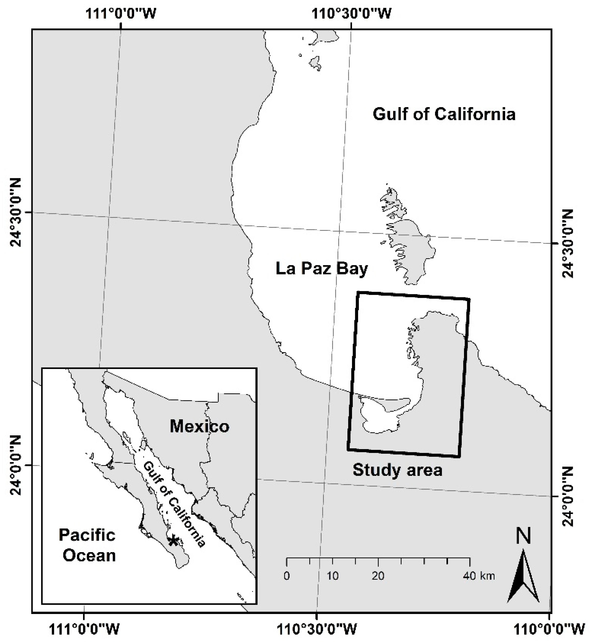
2.1. Study Area

La Paz Bay (Figure 1) consists of a mosaic of coastal habitat types; to the south of the study area is a coastal lagoon that is protected from currents by a sandbar and has areas of dunes and sandy beaches. In the interior of the lagoon, there are vast areas of tidal flats and silt-sandy beaches coupled with areas of mangroves used as nursery habitat for a diverse ichthyofauna [28]. The geomorphology of La Paz lagoon represents a depression with fine-textured sediments (silts and very fine sands) mainly of terrigenous origin and siliciclastic composition, made up of fragments of volcanic rock, quartz-feldspars, and heavy minerals of granitic rocks that come from the discharges from adjacent basins [29].
Conversely, the coastline of the northern portion presents irregular geomorphology due to volcanic rocks that rise under the tectonic conditions of the Gulf of California extension [30]. This topography fosters areas with relatively high slopes forming cliffs and some rocky shore and rocky reef areas on the seabed where coral colonies live; all these habitat types have cryptic fishes. There are also several additional inlets with sandy beaches of calcareous biogenic sedimentation, a rare condition for the eastern Pacific [31] coupled with mangrove habitats.
The seabed is dominated by unconsolidated sediments of carbonate and siliclasts-carbonates of terrigenous and biogenic origin [29,31,32]. The sediments are composed of a wide variety of textures ranging from fine silts to very coarse sands on average, with 2% to 95% percentage variation of carbonates [33]. The high carbonate sediments (>90%) are derived from the settlement of patches of benthic rhodoliths and coral colonies and these are associated with a significant concentration of biodiversity [34]. To a lesser extent, but of great relevance, is the seasonal recruitment of seaweed across the coastal zone.
Nearly 300 species of fish have been documented within the study area [25,35], including the distribution of at least 18 endemic species of fish [36]. There are 11 areas for conservation with the BPNA recognized by UNESCO as a world heritage site, two Ramsar sites (Humedal Balandra and Humedal El Mogote-Ensenada de La Paz), and two priority areas for conservation (Bird Conservation Importance Area Ensenada de La Paz and Priority Marine Region Insular Complex of Baja California Sur [33,37] (Figure S1 supplementary information). Despite these designations, the BPNA is the only one that has a marine management plan within the study area [27]. In Mexico, the decrees of protected areas represent the first step for conservation and do not guarantee full protection; however, these areas require an assessment and can be contrasted with highly important marine spaces such as hotspots.

2.2. Methods

For the marine environment, several methodologies have been developed [22] that attempt to approximate the distribution areas of species and the selection of one depends primarily on the nature of the input data: occurrences and environmental layers. Regarding the occurrences (presence and/or absence) at a given sampling point and considering the nature of fishes, it would be extremely complex to designate a true absence [15]. In this context, some algorithms work with occurrences of “presence-only” type. Within this group of methodologies, the MaxEnt algorithm introduced by Phillips et al. [38,39] is less sensitive compared to other approaches when it has small sample sizes [40,41], demonstrating an acceptable performance [42]. Regarding environmental layers, MaxEnt allows any spatial resolution, coordinate system, and type of variable (qualitative or quantitative). The software is freely accessible, and its management and interpretation of the output maps are relatively simple, and it also presents a significant advance in recent years [43] in the improvement of complementary routines that allow the analysis of a high amount of information during model calibration and evaluation [44,45].
MaxEnt quantifies a probability distribution of maximum entropy [46], constrained to the values of the scenopoetic environmental variables where the species occur [15]. Considering the abiotic conditions of the seabed in the study area and the approach proposed at the relative localized level, high-spatial resolution environmental layers were incorporated. These layers are related to the bottom geomorphology, the sediments (or substrate), and the proximity of fish occurrences from particular habitat types (mangrove and rocky shore, see Table S1 supplementary information).
The methodology consists of four stages: (A) the compilation of the fish occurrence data; (B) environmental layers and calibration area, (C) model calibrations and evaluation; and (D) the development of multi-species and hotspot models.

2.2.1. Occurrence Data

A database with the species and the location of individuals within the study area was integrated into a geographic information system (ArcGIS 10.3) from specialized literature. The main sources of fish data used were Galván-Piña et al. [25], González-Acosta et al. [28], Abitia-Cárdenas et al. [35], Zayas-Álvarez [47], Balart et al. [48], and López-Rasgado et al. [49]. Likewise, the database maintained at the Instituto Politécnico Nacional (http://coleccion.cicimar.ipn.mx/, accessed on 28 December 2019) and additional records from the Global Biodiversity Information Facility [50] were incorporated.
The following criteria were used for the selection of species: historical records between 1975 and 2020 with vouchers of adult specimens (mature) in collections, names recognized in the Integrated Taxonomic Information System (https://www.itis.gov/, accessed on 25 February 2021), and at least 25 presence-only occurrence points for each species. Under these criteria, a set of 217 species was selected from a total of 287, resulting in 8812 total occurrences. MaxEnt software [38,39] uses occurrence data and contrasts them with random points taken from the “background” defined by the total pixels within the selected study area [51]. A brief explanation of the presence–background methods has been reviewed by Sillero and Barbosa [51]. The total occurrences of each species were randomly divided into calibration data (60%) and test data (25%) for the calibration stage. Additionally, a subset of independent data (15%) was reserved (excluded from the calibration) as a complement to the validation of the models, according to Cobos et al. [45].

2.2.2. Environmental Layers and Calibration Area

Eight environmental variables (Table S1, Supplementary Materials) with a high resolution of 0.01 km2 (one-hectare pixels) modified from Urcádiz-Cázares et al. [33] were used in the modelling approach. These layers were selected because they characterize the bay’s abiotic environment with high resolution, and the type of variables have shown acceptable performance in ENM studies [22,41,52,53,54,55,56,57]. These are depth (m), slope inclination (degrees), and aspect (azimuthal degrees of bottom downslope direction), mean grain size (phi), the sediment sorting, and the percentage of calcium carbonate content (seafloor geomorphology layers), and the Euclidean distance (m) from the rocky shore and mangroves habitats. The environmental layers were grouped into three different sets (Table S2, Supplementary Materials) and all were modeled for each species. To define the calibration areas, all of the environmental layers were cut based on reference depth values of −30, −50, −75, and −250 m, according to the maximum depth recorded by the fish [58]. It is important to note that the extent of the calibration areas is geographically limited to the information available. According to Barve et al. [59] the calibration areas should ideally be associated with an accessible area for the species [52], and delimited, for example, by a biogeographic area that allows the geographic range of the species to be predicted. However, it does not intend to predict geographic ranges, but rather focuses on predicting the abiotic suitable areas restricted to the study area, where the species have access. Before calibration modelling, we evaluated environmental layers to avoid correlation and multicollinearity. The Pearson correlation coefficient and the variance inflation factor [59] between variables combinations were calculated in the four areas of calibration and three sets proposed using ENMTools [60] and Rstudio software (https://rstudio.com/, accessed on 5 March 2019). This examination resulted in environmental layers with a low correlation between them (−0.54 < r < 0.72) and an inflation factor of variance < 3.1; therefore, these were considered appropriate for modelling in accordance with Cobos et al. [45].

2.2.3. Model Calibration and Evaluation

For the calibration of the models, we used the kuenm routine [45] in Rstudio that allows the exploration of the parameters in MaxEnt and the building of several models. In this case, the combination of all available features (linear, quadratic, product, threshold, hinge) were assigned, also in combination with 14 values for the regularization multipliers (0.1, 0.2, 0.3, 0.4, 0.5, 0.7, 0.85, 1, 2, 3, 4, 6, 8, and 10) and three different sets of environmental layers (Table S2, supplementary information). This procedure yielded 1302 candidate models for each species.
To select the best species models with statistical significance and minimize possible overfitting [43,61], the candidate models were subjected to five evaluation selection criteria. First, they were subjected to a statistical significance test (p < 0.05) using the area under the curve (AUC) of partial receiver operating characteristic (partial ROC, [58]) through the test data and a bootstrapping of 35% of testing occurrences, 500 interactions, and probabilities were assessed by direct count of the proportion of bootstrap replicates for which the mean AUC ratio was ≤1.0. Partial ROC is appropriate for measuring the performance of ENM that uses only presences occurrences instead of metrics such as full AUC-ROC or TSS (true skill statistics) that are commonly used [62,63,64].
Second, candidate models must have a low omission rate according to a maximum error threshold of 5% that indicates how well the candidate models (using calibration data only) predict the data reserved for testing (as in Anderson et al. [65]) and is the default in kuenm. Third, the candidate models have minimum values of Akaike Information Criterion corrected for small samples (AICc, [44]), indicating how well the models fit the data while penalizing complexity in favor of simple models. The models were constructed using the loglog output, with a bootstrapping (40% of the test data), the jackknife analysis enabled, and 20 replicates to obtain an average model. Fourth, the models that met the above criteria were selected and again subjected to a hypothesis test with the mean AUC ratio, and partial ROC considering the rate of omission error of 0.05, but using the independent data (excluded from calibration). Fifth, the final models of each species were those that met the above criteria, in addition to a low AICc value. These models were finally evaluated with a method insensitive to prevalence with the Continuous Boyce Index (CBI [66]) based on the R routine of Di Cola et al. [67] using independent occurrence data. Only the models that met the tests described above were selected to integrate the hotspot model.

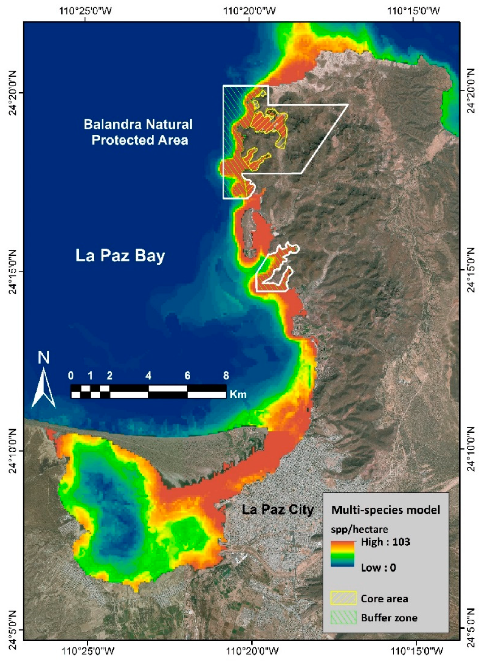
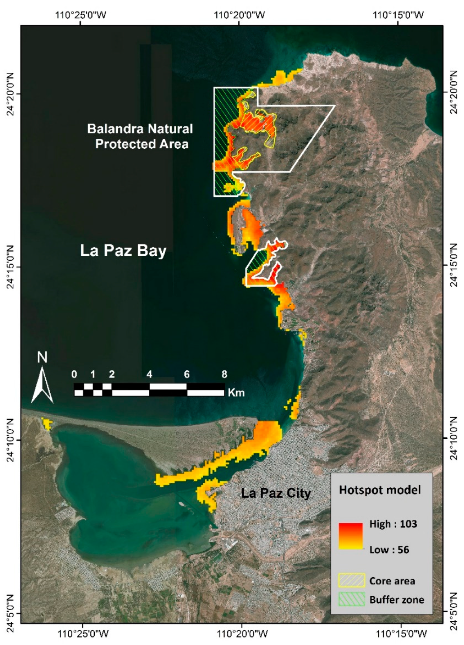
2.2.4. Multi-Species and Hotspot Models

The MaxEnt output showed continuous values from 0 to 1 for each pixel distributed in the geographic space. Final average models were transformed to binary maps [51] assuming a threshold value above that which is suitable for the presence of the species (pixel = 1). The criterion to determine the threshold was the first quartile (Q1) of the set of predicted values at the sites of the presence of the calibration data for each species [15]. The higher the threshold value, the more suitable the values above the threshold in binary maps are.
The transformation to binary maps using GIS allowed the addition of the historically suitable areas of the species to obtain a multi-species map model that indicates the number of endemic fish per pixel (species hectare−1) that can potentially occupy the same habitat space. Considering the univariate distribution of the multi-species map pixels, the values above the 90th percentile were considered here as a hotspot, which contains the geographic area with the highest values of number of species per hectare (species hectare−1). Finally, the hotspot model was contrasted with the geography of the marine conservation areas, specifically with BNPA and its management plan in relation to the limits of its polygons.

3. Results

In total 2.8 × 10⁵ candidate models were generated but only 0.4% were selected with the performance criteria (statistically significant p < 0.05, low omission rate with 0.05 error threshold, and minimum values of AIC). Of these models, 108 were selected for meeting all of the above criteria and having a low CBI value (<0.6), and their performance metrics are shown in Table S2 of the Supplementary Materials. In general, these results indicate that the environmental layers used in this study have a significant capacity to predict abiotically suitable habitats for fish. The environmental layers with the greatest contribution to the prediction of distribution areas were the Euclidean distance from the mangroves habitats with 48.7% and from the rocky shore habitats with 18.5% on average. Likewise, the average grain size and the carbonate content contributed 9.5% and 7.4%, respectively (Figure 2).
By transforming the 108 final models into binary maps and integrating them into the GIS, the multi-species model was constructed (Figure 3). This model indicates the spatial distribution of suitable sites with values from 0 species per hectare to exceptional values of 103 species per hectare.
Using the 90th percentile criterion in the multi-species model (≥60 species per hectare), the hotspot distributions model was established, with the overall area reduced to only 17.8 km2 (Figure 4). The percentage of the distribution of these areas that support the abiotically suitable habitat conditions for high biodiversity within the marine conservation areas is found in Table 1.
More than 68.5% of the hotspot area located within the Humedal El Mogote-Ensenada de La Paz Ramsar Site, the Baja California Sur Insular Complex Priority Marine Area, and the Area of Importance for Bird Conservation does not have an official decree or management plan. Regarding the zoning of the BPNA, 17% of the hotspot is within the “core area” and 23% within the “buffer zone”. The BPNA has had a management plan since 2015 and an official federal decree since 2012. In this area, fish diversity is weakly represented, but the zoning shows high protection of marine organisms exclusively for the core area.

4. Discussion

4.1. Hotspot vs. Marine Conservation Areas

The hotspot model reveals abiotically suitable areas for large numbers of fish (≥60 species per hectare) that should be a priority for conservation policies. Although the Ramsar sites, areas of importance for bird conservation, and the priority marine area (Table 1) cover a large part of the hotspots, these areas remain as “initiatives or proposals” and lack an official decree or management plan that allows protection under a solid regulatory framework. In contrast, the BPNA remains the only instrument with a legal protection framework for marine species. According to BNPA polygons, 60% of the area established as a hotspot (≥60 species per hectare) is outside this area, leaving it vulnerable to infrastructure development and fishing activities in the locality. Within the BPNA, the hotspots occupy 408 hectares (23%) of the buffer zone where the management plan [27] allows activities such as artisanal fishing and infrastructure development with prior authorization by the federal government in legal terms of environmental impact. This implies that the area is potentially vulnerable, even though it is within the protected area. In the same framework, 309 hectares (17%) of the fish hotspot’s area contains the highest level of protection, since it is located in the core area of the BPNA. Protection includes the total conservation of the abiotic environment and biological communities [27]. The management plan no species extraction is allowed in core area, and the development of infrastructure is not allowed.
Delimitation of hotspots or areas featuring exceptional biodiversity is a promising approach to designated areas of priority conservation [8,68]. It has been shown that among large carnivorous species, which constantly move, the conservation requires a combined strategy incorporating the conservation of hotspots or core habitat areas, the linkages between them, and mitigation of human–wildlife conflict [69]. While species conservation requires a holistic approach, it is important to note that the loss of species and habitats is occurring faster than the more modest conservation strategies are being implemented. In this way, the delimitation of the hotspots can be considered as a basic and achievable starting point for species conservation. This delimitation should be followed or if possible accompanied by ecological analyses of the species in order to determine, understand and protect the links between hotspots, the areas that function as nurseries for the hotspot biodiversity, as well as determine and mitigate the areas of human–wildlife conflict.
Our results contribute to the recognition of high fish biodiversity within the BPNA but the current management plan only lists 56 fish species. This work establishes the spatial distribution for 108 species of the 217 documented in the larger study region, with 18 endemic species of the Mexican marine territory [36]. Since the existing legal framework of conservation rigorously protects only 17% of the hotspot area, we suggest a few options to protect these valuable resources. First, expansion of the BPNA to incorporate the documented hotspots and increase the core area that contributes to overall conservation potential; second, create new areas (by municipal, state, or federal orders) for the protection of these hotspots where a high richness of marine species converges; and third, decree a management plan for Ramsar sites, for the area of importance for bird conservation, or for the priority marine area where the proposed hotspot is explicitly included.
This information can be used to guide local economic development patterns spatially based on enhanced environmental impact policies that includes economically-viable ecotourism activities (i.e., scuba diving, snorkeling, photography, the viewing of marine fauna, monitoring, etc.). We suggest incorporation of these important areas into the current management plan or into future conservation plans and policies, as incorporation and protection of these species-rich areas will attract sustainable economic income for the region.

4.2. What Do the Models Indicate?

The interpretation of ecological niche models is rooted in the biological and ecological context of both spatio–temporal scales. It is recognized that fish are dynamic and that the different stages in their biological cycles exhibit different behavioral responses and distribution patterns relative to habitat type and abiotic conditions. For example, in the adult stage many fish species move to different areas to feed, reproduce, and find spawning or refuge areas [28]. The proposed models were constructed using only adult specimens without considering the ontogenetic–ecological roles or functions; therefore, the modeled areas are not specific for a particular role/function but a general occurrence that includes all the possibilities of the mature stage.
In our study, interpreting our models requires an understanding that their construction comes only from historically acquired data (1975–2020) collected in different seasons and by different authors. MaxEnt has been used to develop such distribution models for a number of taxa [13,18,19,20] with input data from a variety of sources (e.g., museum records, open access publications, and long-term data sets). However, in some cases, these distribution maps may not represent approximations of the current distribution. This historical data implies that the models do not document seasonal or decadal changes in the distribution, richness, or abundance of the species across the period studied or potential distribution changes due to over-exploitation or environmental impacts, but rather incorporates all the available information into a single distribution map and calculations of areas outside the currently protected area. In this way, the historical occurrences of the fish will show those habitats associated with abiotically suitable areas that are with greater probability occupied compared to other areas, leaving aside these important dynamics.
Moreover, it must be clear that no ENM faithfully represents the occupied area (current or real) of a species. MaxEnt’s output represents suitable sites based on abiotic information alone. However, the resolution of the study area is small enough to consider it as an accessible area for all species; that is, the abiotically ideal area is within the accessible area [15]. In this way, we interpret the modeled area as an abiotically suitable area nested within adjacent and larger occupied areas.
Geographically demonstrating multi-species biological interactions is a widespread problem in ENM [15]. Therefore, the models are limited to predicting the abiotically suitable areas (as an underestimated part of the occupied area) for the general and historical occurrence of adult fishes. The information generated in our multi-species and hotspot models is extremely useful; locating and prioritizing these hotspot areas where the ideal sites for the species exist is vital for conservation purposes.
One of the most important limitations in this study is that the calibration areas are limited to a geographic extension available in this important area of ichthyofaunal diversity. Barve et al. [59] suggest that the calibration areas should consider a hypothetical accessible area for the species that ideally considers an extension similar to the possible geographic range of the species, but this is valid when looking to predict the geographic range. In this study, we seek to evaluate conservation areas with sufficient detail in spatial resolution that allows reaching conclusions exclusive to the extension and not beyond them. Despite this limitation, our rigorously evaluated models indicate about 48% of the initially documented species presented acceptable performance.

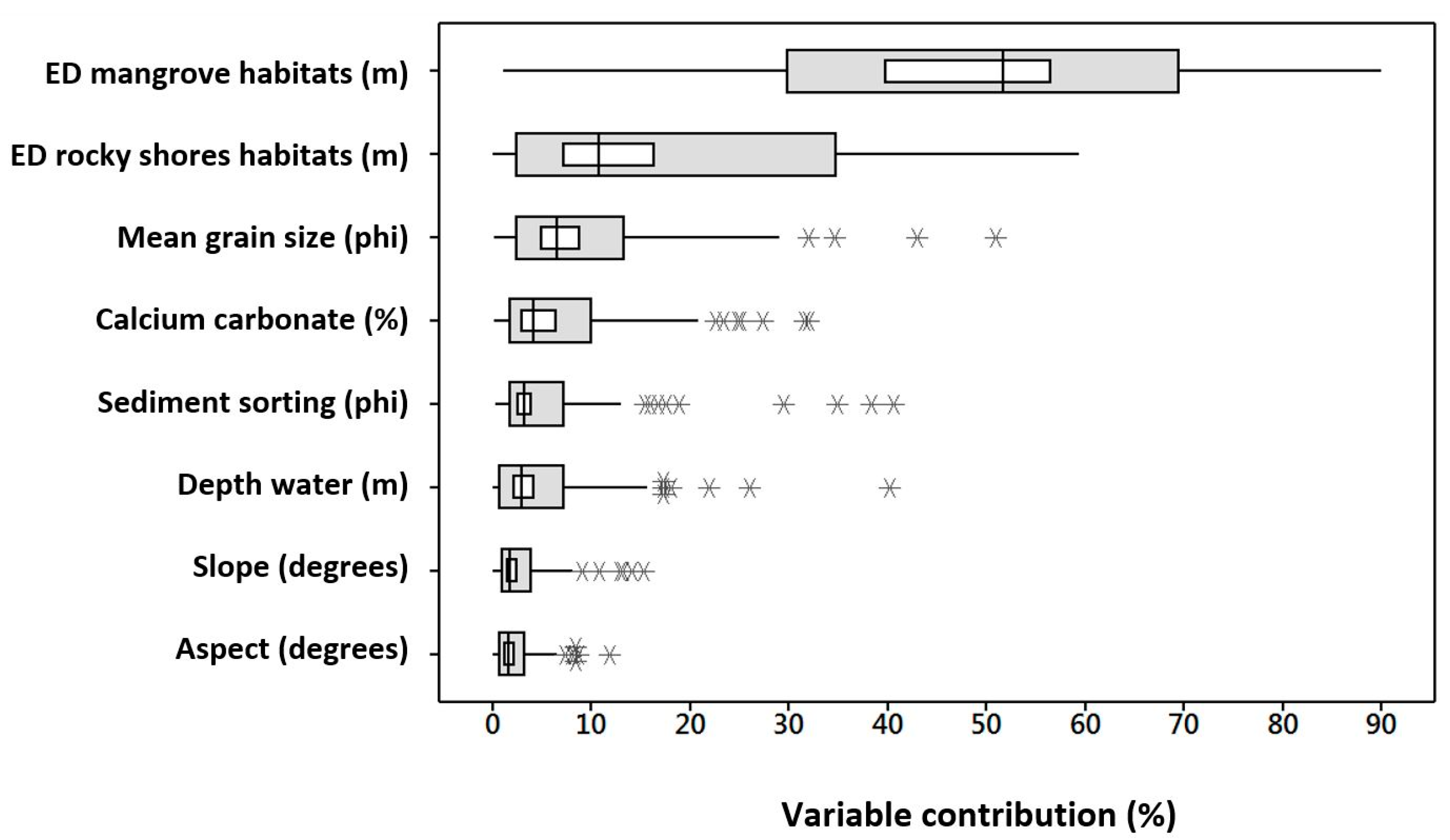
4.3. Variables and Scales

We recognize that variables such as sea surface temperature and chlorophyll concentration are relevant for the distribution of fish species [70] in neritic and pelagic environments [71]. These variables are a direct type since they have a relationship with the physiological tolerance of organisms to abiotic factors [15,67], and particularly chlorophyll, with areas of productivity. These types of variables are useful for studies with a wide geographic range, with regional or global extensions [22] since the pixel resolution of remote sensors has dimensions, e.g., of 1.0 km2 with global availability. For approximations of local extensions such as this study, a higher spatial resolution is required, and these variables are often not available at this scale. This study has implemented indirect high-resolution abiotic variables [22,52] to associate the presence of fish with abiotic conditions related to the geomorphology of the bottom and the substrate, as well as the distance from the mangrove and rocky shore habitats, conditions that characterize this particular coastal zone and models support acceptable performances.

4.4. Impact and Applications

The identification of the areas with the highest ichthyofaunal biodiversity is essential for the establishment and evaluation of marine areas for conservation. In a recent review, Robinson et al. [22] noted that only 63 studies of marine fishes have used ENM approaches between 1950 and 2016, of which 89% are on a regional scale and only 22% involve conservation issues. Obviously, studies based on regional or global scales tend to be oriented to a clearer understanding of the geographic range of the species or their possible changes in distribution derived from global warming scenarios.
In contrast, high-resolution layers in a local framework allow the association of areas of importance with conservation priorities, which generally do not occur on a regional scale. In this sense, there are three studies that highlight high resolution conservation maps. First, Schmiing et al. [52] determined the richness of 20 fish species in the Azores Archipelago and delineated the most important areas in the coastal zone. Second, Leathwick et al. [72] predicted fish distribution in New Zealand and reported maximum richness at 24 fish/pixel. Finally, Moore et al. [73] proposed a solid approach for the management of their fishery based on a detailed distribution of three commercial fish species.
This study establishes the unprecedented distribution of hotspots for the southern Gulf of California. The abiotically suitable areas of fish species were linked to the abiotic conditions, and finally to the current legal framework established for the protection and conservation of the marine environment. Additionally, it is highlighted that the methodological scheme was low cost and is transferable to other groups of marine species; therefore, it could be very useful for coastal zone management professionals, especially for conservation purposes.

Supplementary Materials

The following are available online at https://0-www-mdpi-com.brum.beds.ac.uk/article/10.3390/d13050212/s1, Figure S1: Marine conservation areas within study area, Table S1: Linking habitat and abiotic conditions to fish presence in ecological niche modelling and examples [74,75,76,77,78,79,80], Table S2: Environmental layers (variables) used for calibration. ED = Euclidean distances from specific habitat types, Table S3: Species and their final model evaluation performed with test occurrences and independent data. M AUC r = Mean AUC ratio, p ROC = Partial ROC, OR = omission rate, AICc = Akaike Information Criteria corrected, CBI = continuous Boyce Index. Discarded models**.

Author Contributions

Conceptualization, F.J.U.-C., V.H.C.-E., and A.O.-R.; methodology, F.J.U.-C., E.M.-E., A.B.E.-G., J.M.B.-S., and A.D.P.-M.; validation, F.J.U.-C., E.M.-E., A.D.P.-M., and A.B.E.-G.; formal analysis, F.J.U.-C. and S.S.G.-P.; investigation, F.J.U.-C., V.H.C.-E., J.M.B.-S., and A.O.-R.; resources, F.J.U.-C., V.H.C.-E., S.S.G.-P., and A.O.-R.; data curation, F.J.U.-C.; writing—original draft preparation, F.J.U.-C., V.H.C.-E., R.A.-M., and M.S.P.; writing—review and editing, F.J.U.-C., V.H.C.-E., R.A.-M., M.S.P., and S.S.G.-P.; supervision, F.J.U.-C., V.H.C.-E., and A.O.-R.; funding acquisition, F.J.U.-C. and A.O.-R. All authors have read and agreed to the published version of the manuscript.

Funding

F.J. Urcádiz-Cazares is fellow recipient of CONACyT grant “Estancias posdoctorales por México”. This study was accomplished with the support of the projects IPN-SIP/202110127, Thematic Networks 293368 and Basic Sciences 251919 of CONACyT. V.H. Cruz-Escalona is grateful for the support from Estímulos al Desempeño de los Investigadores (EDI) and Comisión de Operación y Fomento de Actividades Académicas (COFAA) IPN. V. H. Cruz-Escalona, R. Aguilar-Medrano, E. Marín-Enríquez, and A. Ortega-Rubio are fellow recipients of the Sistema Nacional de Investigadores (CONACyT-SNI) México.

Institutional Review Board Statement

Not applicable.

Informed Consent Statement

Not applicable.

Data Availability Statement

Not applicable.

Acknowledgments

We appreciate the comments and support from Maximiliano Cristaldi and Arely Ornelas Vargas to develop this work.

Conflicts of Interest

The authors declare that they have no conflict of interest.

References

  1. Girardello, M.; Santangeli, A.; Mori, E.; Chapman, A.; Fattorini, S.; Naidoo, R.; Bertolino, S.; Svenning, J.-C. Global synergies and trade-off between multiple dimensions of biodiversity and ecosystem services. Sci. Rep. 2019, 9, 5636. [Google Scholar] [CrossRef]
  2. Brooks, T.M.; Mittermeier, R.A.; da Fonseca, G.A.; Gerlach, J.; Hoffmann, M.; Lamoreux, J.F.; Mittermeier, C.G.; Pilgrim, J.D.; Rodrigues, A.S. Global biodiversity conservation priorities. Science 2006, 313, 58–61. [Google Scholar] [CrossRef] [Green Version]
  3. Selig, E.R.; Turner, W.R.; Troeng, S.; Wallace, B.P.; Halpern, B.S.; Kaschner, K.; Lascelles, B.G.; Carpenter, K.E.; Mitter-meir, R.A. Global priorities for marine biodiversity conservation. PLoS ONE 2014, 9, e82898. [Google Scholar] [CrossRef]
  4. Mora, C.; Titensor, D.P.; Adl, S.; Simspn, A.G.B.; Worm, B. How many species are there on Earth and in the ocean? PLoS Biol. 2011, 9, 1–8. [Google Scholar] [CrossRef] [PubMed] [Green Version]
  5. Worm, B.; Barbier, E.B.; Beaumont, N.; Duffy, J.E.; Folke, C.; Halpern, B.S.; Jackson, J.B.C.; Lotze, H.K.; Micheli, F.; Pa-Lumbi, S.R.; et al. Impacts of biodiversity loss on ocean ecosystem services. Science 2006, 314, 787–790. [Google Scholar] [CrossRef] [PubMed] [Green Version]
  6. Hoegh-Guldberg, O.; Bruno, J.F. The impact of climate change on the world’s marine ecosystems. Science 2010, 328, 1523–1528. [Google Scholar] [CrossRef] [PubMed]
  7. Kano, Y.; Dudgeon, D.; Nam, S.; Samejima, H.; Watanabe, K.; Grudpan, C.; Magtoon, W.; Musikasinthorn, P.; Thanh Nguyen, P.; Praxaysonbath, B.; et al. Impacts of dams and global warming on fish biodiversity in the Indo-Burma hotspot. PLoS ONE 2016, 11, e0160151. [Google Scholar] [CrossRef] [Green Version]
  8. Myers, N.; Mittermeier, R.A.; Mittermeier, C.G.; da Fonseca, G.A.; Kent, J. Biodiversity hotspots for conservation priorities. Nature 2000, 403, 853–858. [Google Scholar] [CrossRef]
  9. Mittermeier, R.A.; Turner, W.R.; Larsen, F.W.; Brooks, T.M.; Gascon, C. Global biodiversity conservation: The critical role of hotspots. In Biodiversity Hotspots; Zachos, F.E., Habel, J.C., Eds.; Springer Publishers: London, UK, 2011; pp. 3–22. [Google Scholar]
  10. Cañadas, E.M.; Fenu, G.; Peñas, J.; Lorite, J.; Mattana, E.; Bacchetta, G. Hotspots within hotspots: Endemic plant richness, environmental drivers, and implications for conservation. Biol. Conserv. 2014, 170, 282–291. [Google Scholar] [CrossRef]
  11. Tittensor, D.P.; Mora, C.; Walter, J.; Lotze, W.; Ricard, D.; Berghe, E.V.; Worm, B. Global patterns and predictors of marine biodiversity across taxa. Nature 2010, 466, 1098–1101. [Google Scholar] [CrossRef] [PubMed]
  12. Stuart-Smith, R.D.; Bates, A.E.; Lefcheck, J.S.; Duffy, J.E.; Baker, S.C.; Thomson, R.J.; Stuart-Smith, J.F.; Hill, N.A.; Kinin-month, S.J.; Airoldi, L.; et al. Integrating abundance and functional traits reveals new global hotspots of fish diversity. Nature 2013, 501, 539–542. [Google Scholar] [CrossRef]
  13. McMahan, D.; Fuentes-Montejo, C.E.; Ginger, L.; Carrasco, J.C.; Chakrabarty, P.; Matamoros, W.A. Climate change models predict decreases in the range of a microendemic freshwater fish in Honduras. Sci. Rep. 2020, 10, 12693. [Google Scholar] [CrossRef]
  14. Jetz, W.; McPherson, J.M.; Guralnick, R.P. Integrating biodiversity distribution knowledge: Toward a global map of life. Trends Ecol. Evol. 2012, 27, 151–159. [Google Scholar] [CrossRef]
  15. Peterson, A.T.; Soberón, J.; Pearson, R.G.; Anderson, R.P.; Martínez-Meyer, E.; Nakamura, M.; Bastos Araújo, M. Ecological Niche and Geographic Distribution; Princeton University Press: Princeton, NJ, USA, 2011; 316 p. [Google Scholar]
  16. Teixeira, H.; Berg, T.; Uusitalo, L.; Fürhaupter, K.; Heiskanen, A.-S.; Mazik, K.; Lynam, C.P.; Neville, S.; Rodriguez, J.G.; Papadopolou, N.; et al. A catalogue of marine biodiversity indicators. Front. Mar. Sci. 2016, 207, 1–16. [Google Scholar] [CrossRef] [Green Version]
  17. Newbold, T.; Reader, T.; El-Gabbas, A.; Berg, W.; Shohdi, W.M.; Zalat, S.; Baha El Din, S.; Gilbert, F. Testing the accuracy of species distribution models using species records from a new field survey. Oikos 2010, 119, 1326–1334. [Google Scholar] [CrossRef]
  18. Baltensperger, A.P.; Huettmann, F. Predictive spatial niche and biodiversity hotspot models for small mammal communities in Alaska: Applying machine-learning to conservation planning. Landsc. Ecol. 2015, 30, 681–697. [Google Scholar] [CrossRef]
  19. Cooper-Bohannon, R.; Rebelo, H.; Jones, G.; Cotterill, F.; Monadjem, A.; Schoeman, M.C.; Taylor, P.; Park, K. Predicting bat distributions and diversity hotspots in southern Africa. Hystrix Ital. J. Mamm. 2016, 27, e11722. [Google Scholar] [CrossRef]
  20. Smith, J.N.; Kelly, N.; Renner, I.W. Validation of presence-only models for conservation planning and the application to whales in a multiple-use marine park. Ecol. Appl. 2020, 31, e02214. [Google Scholar] [CrossRef]
  21. Zhang, H.; Zhao, H. Study on rare and endangered plants under climate: Maxent modeling for identifying hot spots in northwest China. CERNE 2021, 27, e-102667. [Google Scholar] [CrossRef]
  22. Robinson, N.M.; Nelson, W.A.; Cosello, M.; Sutherland, J.; Lundquist, C. A systematic review of marine-based species distribution models (SDMs) with recommendations for best practice. Front. Mar. Sci. 2017, 421, 1–11. [Google Scholar] [CrossRef] [Green Version]
  23. Ahmed, S.E.; McInerny, G.; O’Hara, K.; Harper, R.; Salido, L.; Emmott, S.; Joppa, L.N. Scientists and software–surveying the species distribution modelling community. Divers. Distrib. 2015, 21, 258–267. [Google Scholar] [CrossRef]
  24. González-Acosta, A.F.; Balart, E.F.; Ruiz-Campos, G.; Espinosa Pérez, H.; Cruz-Escalona, V.H.; Hernández-López, A. Diversidad y conservación de los peces de la bahía de La Paz, Baja California Sur, México. Rev. Mex. Biodiver. 2018, 89, 705–740. [Google Scholar] [CrossRef]
  25. Galván-Piña, V.H.; Galván-Magaña, F.; Abitia-Cárdenas, L.A.; Gutiérrez-Sánchez, F.J.; Rodríguez-Romero, J. Seasonal structure of fish assemblages in rocky and sandy habitats in Bahía de La Paz, Mexico. Bull. Mar. Sci. 2003, 72, 19–35. [Google Scholar]
  26. Diario Oficial de la Federación. Decreto por el que se Declara Área Natural Protegida, con el Carácter de Área de Protección de Flora y Fauna, la Región Conocida como Balandra, Localizada en el Municipio de La Paz, en el Estado de Baja California Sur; Secretaría de Medio Ambiente y Recursos Naturales: Ciudad de México, Mexico, 2012. [Google Scholar]
  27. Diario Oficial de la Federación. Resumen del Programa de Manejo del Área de Protección de Flora y Fauna Balandra; Secretaría de Medio Ambiente y Recursos Naturales: Ciudad de Mexico, Mexico, 2015. [Google Scholar]
  28. González-Acosta, A.F.; De-la-Cruz-Agüero, G.; De-la-Cruz-Agüero, J.; Ruiz-Campos, G. Ictiofauna asociada al manglar del estero El Conchalito, Ensenada de La Paz, B.C.S., México. CICIMAR Oceán. 1999, 14, 121–131. [Google Scholar]
  29. Choumiline, K.; Godínez-Orta, L.; Nikolaeva, A.; Derkachev, A.; Shumilin, E. Evaluation of contribution sources for the sediments of the La Paz Lagoon based on statistical treatment of the mineralogy of their heavy fraction and surrounding rock and drainage basin characteristics. Bol. Soc. Geol. Mex. 2009, 61, 97–109. [Google Scholar] [CrossRef]
  30. Nava-Sánchez, E.H.; Gorsline, D.S.; Molina-Cruz, A. The Baja California peninsula borderland: Structural and sedimentological characteristics. Sediment. Geol. 2001, 144, 63–82. [Google Scholar] [CrossRef]
  31. Halfar, J.; Ingle, J., Jr.; Godínez-Orta, L. Modern non-tropical mixed carbonate-siliciclastic sediments and environments of the southwestern Gulf of California, Mexico. Sediment. Geol. 2004, 165, 93–115. [Google Scholar] [CrossRef]
  32. Silverberg, N.; Aguirre-Bahena, F.; Mucci, A. Time-series measurements of settling particulate matter in Alfonso Basin, La Paz Bay, southwestern Gulf of California. Cont. Shelf Res. 2014, 84, 169–187. [Google Scholar] [CrossRef]
  33. Urcádiz-Cázares, F.J.; Cruz-Escalona, V.H.; Nava-Sánchez, E.; Ortega-Rubio, A. Clasificación de unidades del fondo marino a partir de la distribución espacial de los sedimentos superficiales de la Bahía de La Paz, Golfo de California. Hidrobiológica 2017, 27, 399–409. [Google Scholar] [CrossRef]
  34. Steller, D.L.; Riosmena-Rodríguez, R.; Foster, M.S.; Roberts, C.A. Rhodolith bed diversity in the Gulf of California: The importance of rhodoliths structure and consequences of disturbance. Aquat. Conserv. 2003, 13, 5–20. [Google Scholar] [CrossRef]
  35. Abitia-Cárdenas, L.A.; Rodríguez-Romero, J.; Galván-Magaña, F.; De-la-Cruz-Agüero, J.; Chávez-Ramos, H. Lista sistemática de la ictiofauna de Bahía de La Paz, Baja California Sur, México. Cienc. Mar. 1994, 20, 159–181. [Google Scholar] [CrossRef] [Green Version]
  36. Urcádiz-Cázares, F.J.; Cruz-Escalona, V.H.; Peterson, M.; Marín-Enríquez, M.; González-Acosta, A.F.; Martínez-Flores, G.; Hernández-Carmona, G.H.; Aguilar Medrano, R.; Del Pino-Machado, A.; Ortega-Rubio, A. Ecological niche modelling of endemic fish within La Paz Bay: Implications for conservation. J. Nat. Conserv. 2021, 60, 125981. [Google Scholar] [CrossRef]
  37. Arriaga Cabrera, L.; Aguilar, V.; Espinoza, J.M. Regiones Prioritarias y Planeación para la Conservación de la Biodiversidad. In: Capital Natural de México. Vol. II: Estado de Conservación y Tendencias de Cambio; CONABIO: Ciudad de México, Mexico, 2009; pp. 433–457. [Google Scholar]
  38. Phillips, S.J.; Anderson, R.P.; Schapire, R.E. Maximum entropy modelling of species geographic distributions. Ecol. Model. 2006, 190, 231–259. [Google Scholar] [CrossRef] [Green Version]
  39. Phillips, S.J.; Anderson, R.P.; Dudík, M.; Schapire, R.E.; Blair, M.R. Opening the black box: An open-source release of Maxent. Ecography 2017, 40, 887–893. [Google Scholar] [CrossRef]
  40. Pearson, G.R.; Raxworthy, C.J.; Nakamura, M.; Peterson, T.A. Predicting species distributions from small numbers of occurrence records: A test case using cryptic geckos in Madagascar. J. Biogeogr. 2007, 34, 102–117. [Google Scholar] [CrossRef]
  41. Monk, J.; Ierodiaconou, D.; Versace, V.L.; Bellgrove, A.; Harvey, E.; Rattray, A.; Laurenson, L.; Quinn, G.P. Habitat suit-ability for marine fishes using presence-only modelling and multibeam sonar. Mar. Ecol. Prog. Ser. 2010, 420, 157–174. [Google Scholar] [CrossRef] [Green Version]
  42. Wisz, M.S.; Hijmans, R.J.; Peterson, A.T.; Graham, C.H.; Guisan, A. Effect of sample size on the performance of species distribution models. Divers. Distrib. 2008, 14, 763–773. [Google Scholar] [CrossRef]
  43. Morales, N.S.; Fernández, I.C.; Baca-González, V. MaxEnt’s parameter configuration and small samples: Are we paying attention to recommendations? A systematic review. PeerJ 2017, 5, e3093. [Google Scholar] [CrossRef]
  44. Warren, D.L.; Seifert, S.N. Ecological niche modeling in Maxent: The importance of model complexity and the performance of model selection criteria. Ecol. Appl. 2011, 21, 335–342. [Google Scholar] [CrossRef] [Green Version]
  45. Cobos, M.E.; Peterson, A.T.; Barve, N.; Osorio-Olvera, L. kuenm: An R package for detailed development of ecological niche models using Maxent. PeerJ 2019, 7, e6281. [Google Scholar] [CrossRef] [PubMed] [Green Version]
  46. Elith, J.; Phillips, S.J.; Hastie, T.; Dudík, M.; Chee, Y.E.; Yates, C.J. A statistical explanation of Maxent for ecologist. Divers. Distrib. 2011, 17, 43–57. [Google Scholar] [CrossRef]
  47. Zayas-Álvarez, J.A. Análisis Temporal de la Estructura Comunitaria de los Peces Crípticos Asociados A un Arrecife Artificial en Punta Diablo, Bahía de La Paz, B.C.S., México. Master’s Thesis, Centro de Investigaciones Biológicas del Noroeste S.C., La Paz, Mexico, 2015. [Google Scholar]
  48. Balart, E.F.; González-Cabello, A.; Romero-Ponce, C.; Zayas-Alvarez, A.; Calderón-Parra, M.; Campos-Dávila, L.; Find-Ley, L.T. Length-weight relationships of cryptic reef fishes from the southwestern Gulf of California, México. J. Appl. Ichthyol. 2006, 22, 316–318. [Google Scholar] [CrossRef]
  49. López-Rasgado, F.J.; Herzka, S.Z.; Del-Monte-Luna, P.; Serviere-Zaragoza, E.; Balart, E.F.; Lluch-Cota, S.E. Fish assemblages in three arid mangrove systems of the Gulf of California: Comparing observations from 1980 and 2010. Bull. Mar. Sci. 2012, 88, 919–945. [Google Scholar] [CrossRef]
  50. GBIF.org. GBIF Occurrence. Available online: https://10.15468/dl.k5mc7e (accessed on 25 February 2021).
  51. Sillero, N.; Barbosa, M. Common mistakes in ecological niche models. Int. J. Geogr. Inf. Syst. 2021, 35, 213–226. [Google Scholar] [CrossRef]
  52. Franklin, J. Mapping Species Distributions: Spatial Inference and Prediction (Ecology, Biodiversity and Conservation); Cambridge University Press: Cambridge, UK, 2009. [Google Scholar]
  53. Schmiing, M.; Diogo, H.; Serrão Santos, R.; Alfonso, P. Assessing hotspots within hotspots to conserve biodiversity and support fisheries management. Mar. Ecol. Prog. Ser. 2014, 513, 187–199. [Google Scholar] [CrossRef]
  54. Austin, M.P.L. Spatial prediction of species distribution: An interface between ecological theory and statistical modelling. Ecol. Model. 2002, 157, 101–118. [Google Scholar] [CrossRef] [Green Version]
  55. Pittman, S.; Brow, K.A. Multi-scale approach for predicting fish species distributions across coral reef seascapes. PLoS ONE 2011, 6, e20583. [Google Scholar] [CrossRef] [PubMed]
  56. Ŝiaulys, A. Empirical Modelling of Macrozoobenthos Species Distribution and Benthic Habitat Quality Assessment. Ph.D. Thesis, Coastal Research and Planning Institute, Klaipèda University, Klaipèda, Lithuania, 2013. [Google Scholar]
  57. Snickarsa, M.; Sundblad, G.; Sandström, A.; Ljunggren, L.; Bergström, U.; Johansson, G.; Mattila, J. Habitat selectivity of a substrate spawning fish: Modelling requirements for the Eurasian perch Perca fluviatilis. Mar. Ecol. Prog. Ser. 2010, 398, 235–243. [Google Scholar] [CrossRef] [Green Version]
  58. Froese, R.; Pauly, D. (Eds.) FishBase. World Wide Web Electronic Publication. 2020. Available online: www.fishbase.org (accessed on 15 January 2020).
  59. Barve, N.; Barve, V.; Jiménez-Valverde, A.; Lira-Noriega, A.; Maher, S.A.; Peterson, A.T.; Soberon, J.; Villalobos, F. The crucial role of the accessible area in ecological niche modeling and species distribution modeling. Ecol. Model. 2011, 222, 1810–1819. [Google Scholar] [CrossRef]
  60. Peterson, A.T.; Pepes, M.; Soberón, J. Rethinking receiver operating characteristic analysis applications in ecological niche modelling. Ecol. Model. 2008, 213, 63–72. [Google Scholar] [CrossRef]
  61. O’Brien, R.M. A caution regarding rules of thumb for variance inflation factors. Qual. Quant. 2007, 41, 673–690. [Google Scholar] [CrossRef]
  62. Warren, D.L.; Matzke, N.; Cardillo, M.; Baumgartner, J.; Beaumont, L.; Huron, N.; Simões, M.; Iglesias, T.L.; Dinnage, R. ENMTools (Software Package). 2019. Available online: https://github.com/danlwarren/ENMTools (accessed on 8 March 2020).
  63. Merow, C.; Smith, M.J.; Silander, J.A. A practical guide to MaxEnt for modeling species’ distributions: What it does, and why input settings matter. Ecography 2013, 36, 1058–1069. [Google Scholar] [CrossRef]
  64. Lobo, J.M.; Jiménez-Valverde, A.; Real, R. AUC: A misleading measure of the performance of predictive distribution models. Glob. Ecol. Biogeogr. 2007, 17, 145–151. [Google Scholar] [CrossRef]
  65. Jiménez-Valverde, A. Insights into the area under the receiver operating characteristic curve (AUC) as a discrimination measure in species distribution modelling. Glob. Ecol. Biogeogr. 2012, 21, 498–507. [Google Scholar] [CrossRef]
  66. Leroy, B.; Delsol, R.; Hugueny, B.; Meynard, C.N.; Barhoumi, C.; Barbet-Massin, M.; Bellard, C. Witho ut quality pres-ence–absence data, discrimination metrics such as TSS can be misleading measures of model performance. J. Biogeogr. 2018, 45, 1–9. [Google Scholar] [CrossRef]
  67. Anderson, R.P.; Lew, D.; Peterson, A.T. Evaluating predictive models of species’ distributions: Criteria for selecting optimal models. Ecol. Model. 2003, 162, 211–232. [Google Scholar] [CrossRef]
  68. Hirzel, A.H.; Le Lay, G.; Helfer, V.; Randin, C.; Guisan, A. Evaluating the ability of habitat suitability models to predict species presence. Ecol. Model. 2006, 199, 142–152. [Google Scholar] [CrossRef]
  69. Di Cola, V.; Broennimann, O.; Petitpierre, B.; Breiner, F.T.; D’Amen, M.; Randin, C.; Engler, R.; Pottier, J.; Pio, D.; Dubuis, A.; et al. ecospat: An R package to support spatial analyses and modeling of species niches and distributions. Ecography 2017, 40, 774–787. [Google Scholar] [CrossRef]
  70. Myers, N. Threatened biotas: ‘Hotspots’ in tropical forests. Environmentalist 1988, 8, 187–208. [Google Scholar] [CrossRef]
  71. Cushman, S.A.; Elliot, N.B.; Bauer, D.; Kesch, K.; Bahaa-el-din, L.; Bothwell, H.; Flyman, M.; Mtare, G.; Macdonald, D.W.; Loveridge, A.J. Prioritizing core areas, corridors and conflict hotspots for lion conservation in southern Africa. PLoS ONE 2018, 13, e0196213. [Google Scholar] [CrossRef]
  72. Trujillo, A.P.; Thurman, H.V. Essentials of Oceanography, 12th ed.; Pearson Education, Inc.: Boston, MA, USA, 2016. [Google Scholar]
  73. Wang, L.; Kerr, L.A.; Record, N.R.; Bridger, E.; Tupper, B.; Mills, K.E.; Armstrong, E.M.; Pershing, A.J. Modeling marine pelagic fish species spatiotemporal distributions utilizing a maximum entropy approach. Fish. Oceanogr. 2018, 27, 571–586. [Google Scholar] [CrossRef]
  74. Leathwick, J.R.; Elith, J.; Francis, M.P.; Hastie, T.; Taylor, P. Variation in demersal fish species richness in the oceans surrounding New Zealand: An analysis using boosted regression trees. Mar. Ecol. Prog. Ser. 2006, 321, 267–281. [Google Scholar] [CrossRef] [Green Version]
  75. Moore, C.; Drazen, J.C.; Radford, B.T.; Kelley, C.; Newman, S.J. Improving essential fish habitat designation to support sustainable ecosystem-based fisheries management. Mar. Policy 2016, 69, 32–41. [Google Scholar] [CrossRef]
  76. Hogarth, P.J. The Biology of Mangroves and Seagrasses; Oxford University Press: Oxford, UK, 2015; p. 389. [Google Scholar]
  77. Little, C.; Williams, G.A.; Trowbridge, C.D. The Biology of Rocky Shores; Oxford University Press: Oxford, UK, 2009; p. 356. [Google Scholar]
  78. Verfaillie, E.; Van-Lancker, V.; Van-Meirvenne, M. Multivariate geostatistics for the predictive modelling of the surficial sand distribution in shelf seas. Cont. Shelf Res. 2006, 26, 2454–2468. [Google Scholar] [CrossRef]
  79. Haris, K.; Chakraborthy, B.; Ingole, B.; Menezes, A.; Srivastava, R. Seabed habitat mapping employing single and multi-beam backscatter data: A case study from the western continental shelf of India. Cont. Shelf Res. 2012, 48, 40–49. [Google Scholar] [CrossRef]
  80. Mora, C. Ecology of Fishes on Coral Reef; Cambridge University Press: Cambridge, UK, 2015. [Google Scholar]
Figure 1. Study area location within La Paz Bay (southern Gulf of California).
Diversity 13 00212 g001
Figure 2. Relative contribution (%) of the environmental layers (variables) to MaxEnt models based on the 108 species. ED = Euclidean distance from specific habitats. ED mangrove and rocky shores habitats are the main variables for abiotically suitable areas predictions.
Diversity 13 00212 g002
Figure 3. Multi-species distribution model. Color scale shows abiotically suitable sites for fish (species per hectare). The white polygon shows Balandra Protected Natural Area.
Diversity 13 00212 g003
Figure 4. Hotspot distribution model. Fish hotspot (≥60 species per hectare) is about 1778 Ha. Only 17% of the hotspot is within the core area of the Balandra Natural Protected Area (yellow polygon). The green polygon corresponds to the buffer zone.
Diversity 13 00212 g004
Table 1. Hotspot area within marine conservation areas and their conservation policy legal status. * Only with international registration. BNPA(BZ): Balandra Natural Protected Area (buffer zone); BNPA(CA): Balandra Natural Protected Area (core area); HBRS: Humedal Balandra Ramsar Site; HEM-ELP-RS: Humedal El Mogote-Ensenada de La Paz Ramsar Site; BCIAELP: Bird Conservation Importance Area Ensenada de La Paz; PMRICBCS: Priority Marine Region Insular Complex of Baja California Sur.
Marine Conservation AreasOfficial DecreeManagement PlanHotspot (Hectares)
BNPA(BZ)YesYes408
BNPA(CA)YesYes309
HBRSNo *No402
HEM-ELP-RSNo *No1249
BCIAELPNoNo1219
PMRICBCSNoNo1778
Publisher’s Note: MDPI stays neutral with regard to jurisdictional claims in published maps and institutional affiliations.

