Article

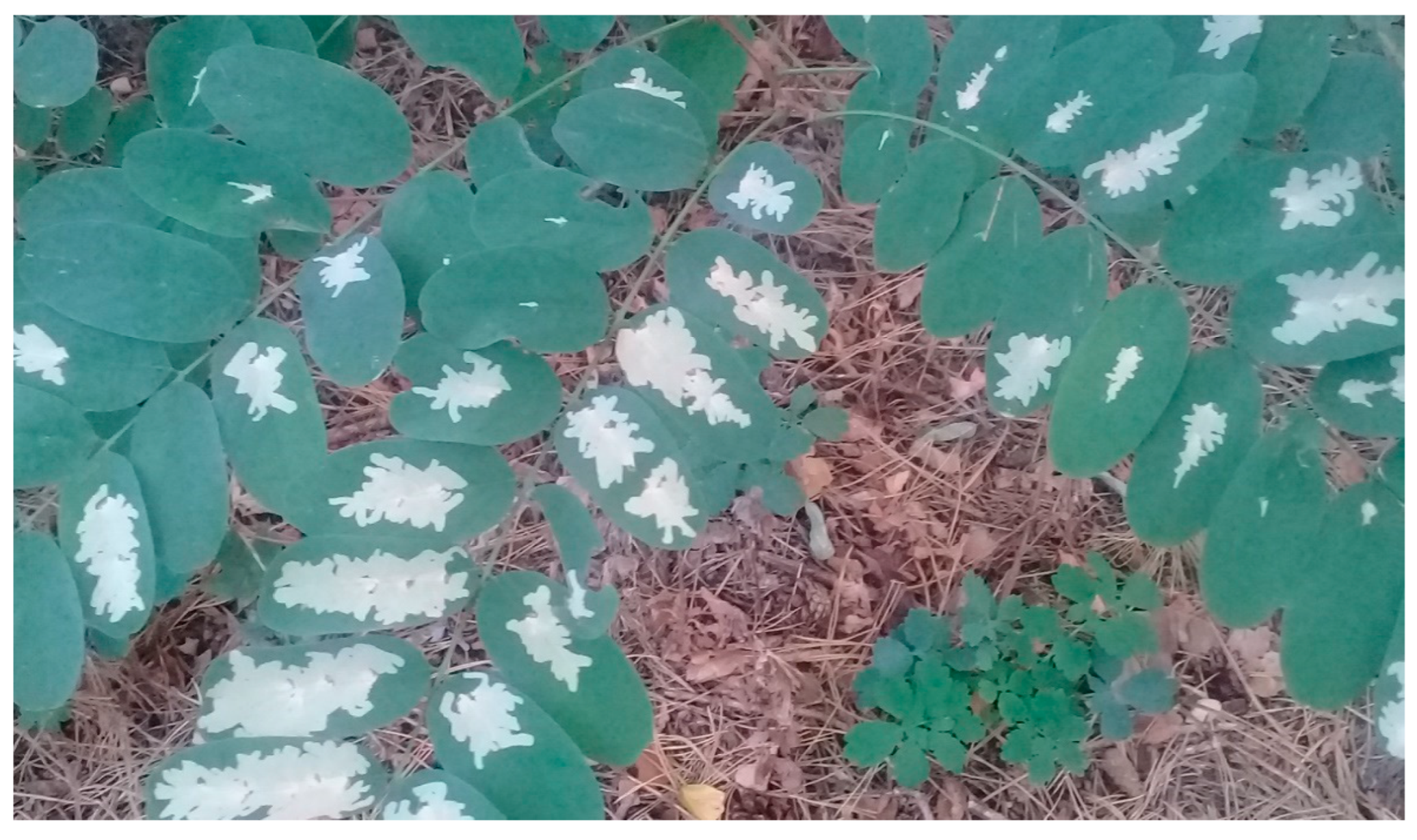
The Spread of the Invasive Locust Digitate Leafminer Parectopa robiniella Clemens, 1863 (Lepidoptera: Gracillariidae) in Europe, with Special Reference to Ukraine

1
I.I. Schmalhausen Institute of Zoology, National Academy of Sciences of Ukraine, 01030 Kyiv, Ukraine
2
Department of Ecology, Institute of Life Sciences and Technologies, Daugavpils University, LV5400 Daugavpils, Latvia
*
Author to whom correspondence should be addressed.
Submission received: 3 July 2022 / Revised: 25 July 2022 / Accepted: 26 July 2022 / Published: 28 July 2022

Abstract

:
The spread and outbreaks of phytophagous pests are often associated with global warming. In addition to economic interest, these species may be of interest in terms of biological indication of climate changes. In this context, we considered the locust digitate leafminer Parectopa robiniella Clemens, 1863 (Lepidoptera: Gracillariidae). This phytophage was first discovered in Europe in 1970 near Milano in Italy. Since then, it has been spreading across the continent. In Ukraine, it was recorded for the first time in 2003. In 2020–2021, we found areas of massive leaf damage caused by the black locust (Robinia pseudoacacia) in locations on Trukhaniv Island in Kyiv and some places in the Kyiv administrative region. Using 1041 georeferenced records of P. robiniella across Europe and a Bayesian additive regression trees algorithm (BART), we modeled the distribution of the moth. Predictors of current climate (WorldClim v.2, CliMond v.1.2 and ENVIREM) and a black locust habitat suitability raster were employed. Sets of SDMs built for P. robiniella with and without the habitat suitability raster for the host tree performed equally well. Amongst the factors that determine the niche of the locust digitate leafminer, most important are temperature-related conditions assumed to facilitate the spread and naturalization of the pest. In Ukraine, the appearance of the moth has coincided with increasing mean annual temperatures. Particularly favorable for the species are areas in the west and south-west of the country, and Transcarpathia. In the near future, the moth could reach locations in Nordic countries, Estonia, the British Isles, Black Sea coastal areas in Turkey, further into Russia, etc.

1. Introduction

Earth’s temperature has risen by 0.08 °C per decade since 1880, and the rate of warming over the past 40 years has been more than twice that: 0.18 °C per decade since 1981 [1]. Numerous studies provide evidence for biological responses to recent climate change [2], and in particular, focused on changes in the distribution and range shifts of species [3,4,5]. For pest insects, it is expected that climate warming will affect both incidence and the geographical extent and intensity of population outbreaks, with potentially severe economic and ecological consequences [6]. In this context, we considered the locust digitate leafminer Parectopa robiniella Clemens, 1863 (Lepidoptera: Gracillariidae), which has been suggested as a model species indicating climate change. It is native to North America, but was accidentally introduced to Italy, where it was first found in Milano in 1970 [7]. The moth has now been recorded in a number of European countries, ranging from Spain to Latvia [8,9,10,11,12,13,14,15,16,17,18,19,20,21]. On average, the spread of the pest occurs at a speed of about 100 km per year [22]. The moth is associated with the black locust (Robinia pseudoacacia L.), a tree introduced to Europe from North America at the beginning of the XVII century for decorative reasons, and to Ukraine it was brought at the end of the XVIII century [19]. In some countries, such as Romania and Hungary, it has become an essential landscape element [23,24]. In Ukraine too, particularly in the south, the tree has been widely cultivated for variety of purposes. R. pseudoacacia is considered an excellent plant for growing in highly disturbed areas as an erosion control plant [25], and the black locust is also a major honey-producing plant [26].
In Ukraine, the species was recorded for the first time in Kyiv and Chernivtsi (a regional capital in the south-west of the country) in 2003 [27]. In 2020, we discovered an extensive outbreak of the pest on Trukhaniv Island, a floodplain island located within the city boundaries of Kyiv. In 2021 a second outbreaj was found in Obukhiv District, some 50 km south of the capital city. P. robiniella larvae develop in chambers (“mines”) inside the leaves, causing “finger-like” excavations all around the margins of the central blotch of the mine [28] (Figure 1). Strong damage to the leaves leads to reduction of the black locust’s flowering period and a decrease in nectar production, which adversely affects the honey harvest [29].
Although P. robiniella is now widely prevalent in Europe, there are heterogeneities in the pest’s distribution that are likely linked to environmental parameters. In this respect, species distribution models (SDMs) have proven to be useful tools for predicting pest distribution and elucidating the importance of a wide range of environmental covariates that are considered to affect pest species occurrence [30]. Using SDMs, our objective was to: (1) identify areas of habitat suitability for the moth; (2) identify conditions that constrain the geographic distribution of P. robiniella in Europe, particularly in Ukraine; (3) against the background of the appearance of P. robiniella in Kyiv, verify the assumption that positive dynamics of the average annual temperature in the city could act as one of the possible factors promoting the invasion of this species.

2. Materials and Methods

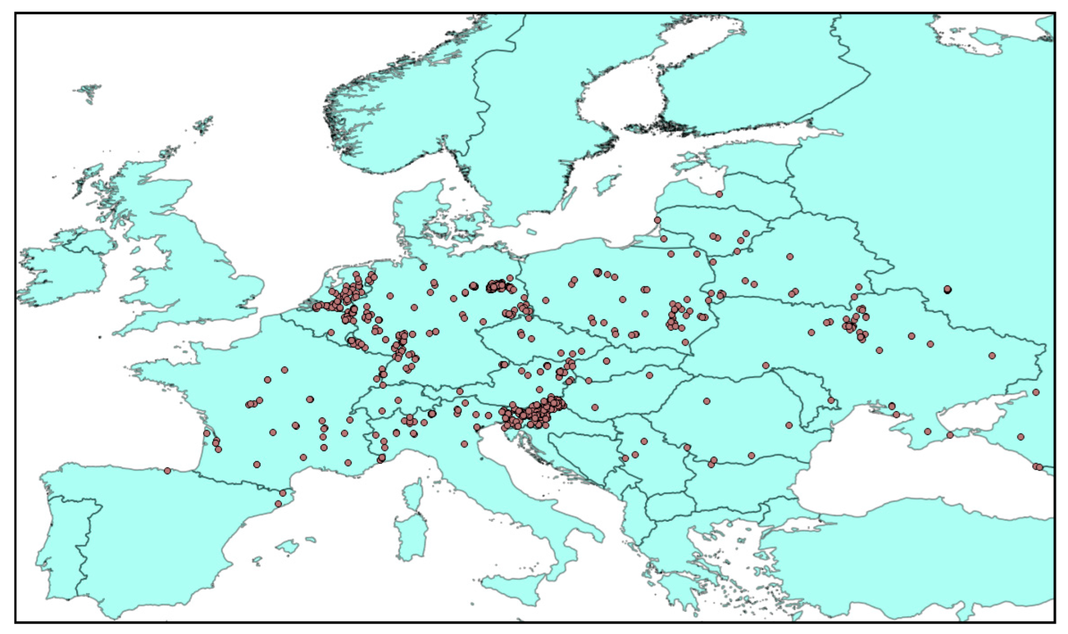
2.1. Occurrence Records and Environmental Variables

As input, SDMs require georeferenced biodiversity observations. Localities for P. robiniella were gathered from GBIF [31,32], records found in the literature (see https://dabasdati.lv/en/ [13,14,15,16,17,18,19,20,21]), and our personal field surveys. As many uncertainties are associated with SDM projections, particularly when it comes to building a SDM for a species expanding its home range in a new area [33], we used for the analysis only records of European localities. In its introduced range, black locust grows successfully in climatic conditions that are quite different from those of its native range [34]. This was for us an additional reason to focus on the invasive range of the pest, which is tightly associated with the tree host. SDMs commonly utilize associations between environmental variables and known species occurrence records to identify environmental conditions within which populations can be maintained. SDMs extrapolate in situ habitats in both space and time to obtain spatially explicit and continuous surfaces indicating the probability of species occurrence [35]. SDMs are primarily climate-driven, meaning that the variables used to develop them typically portray climatic factors [36]. This makes sense because climate is a chief driver of environmental suitability [30,36,37].
Information on the bioclimatic parameters was collected as raster layers from three climatic data bases and used separately for building the anticipated SDMs and checking their performances for both the moth and host tree.
From the WorldClim website (http://www.worldclim.com/version2 (accessed on 21 January 2022)), 19 bioclimatic variables, indicating general trends in precipitation and temperature, including extremes and the seasonality of temperature [38], were downloaded at 2.5′ resolution; however, we excluded four variables (Bio 8, Bio 9, Bio 18, and Bio 19) owing to their known spatial artifacts, following the protocol implemented in previous similar studies [39,40]. Other “Quarter” variables were removed too, because they are correlated a lot with monthly values and carry large amounts of redundant information.
CliMond v.1.2 datasets were downloaded from https://www.climond.org/ at 10′ resolution. These included the core set of 19 bioclimatic variables (temperature and precipitation) and an extended set of 16 additional variables (solar radiation and soil moisture) [41]. As in the previous case, quarterly variables were discarded.
In this study, we used for modelling purposes a set of 16 climatic and 2 topographic variables (the ENVIREM dataset, downloaded from http://envirem.github.io (accessed on 21 January 2022) in a 2.5′ resolution), which were found by recently reconsidering biological significance; many of them are likely to have direct relevance to ecological or physiological processes determining species distributions [42,43]. These variables are worth consideration in species distribution modeling applications, especially as many of the variables (in particular, potential evapotranspiration) have direct links to processes that are important for species ecology. The included topographic variables are potentially important too, because they can modify the effects of the climate descriptors.
Although environmental conditions may predict a species’ potential geographic distribution broadly, climatic factors typically used to represent those conditions are questionable surrogates for factors such as host availability [30]. Therefore, we included in each set of the used environmental predictors a raster reflecting the habitat suitability of the black locust in Europe. For this purpose, occurrences were extracted from the GBIF database [44].
Following M. A. Nuñez and K. A. Medley [45], we measured the spatial autocorrelation of occurrences by calculating Moran’s I for multiple distance classes using the SAM v4.0 software [46]; values < 0.3 were considered acceptable for building meaningful SDMs [47]. The extent used during the niche modeling process has a profound influence on the outcome of the model [36]. In other words, if the extent under consideration is too limited to be accessible to the species area via dispersal, the importance of coarse-resolution factors such as climate in delimiting species’ distributions may be underestimated [47].

2.2. Modelling Procedure
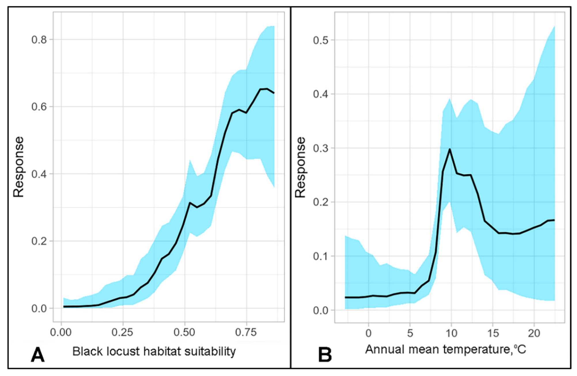
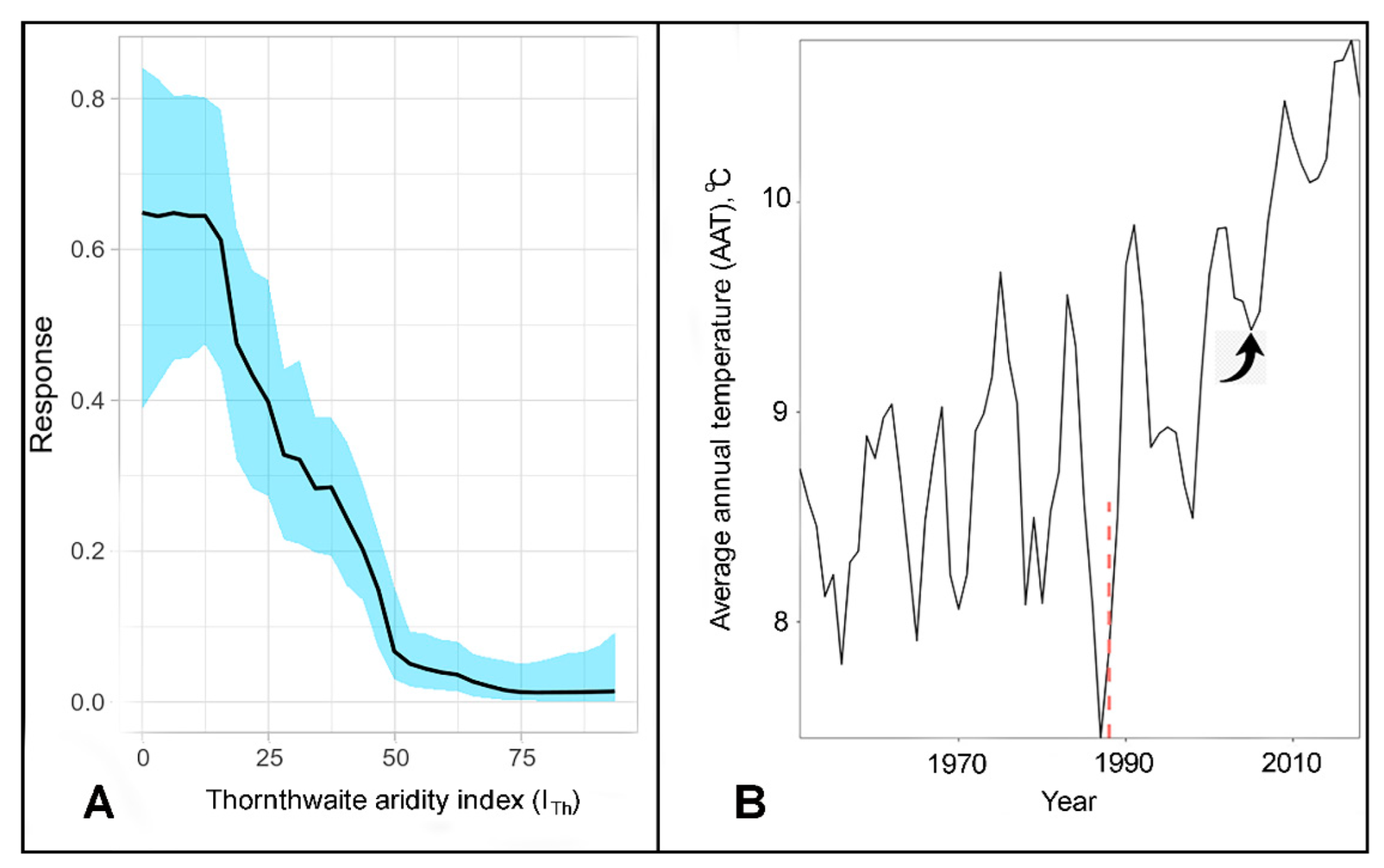
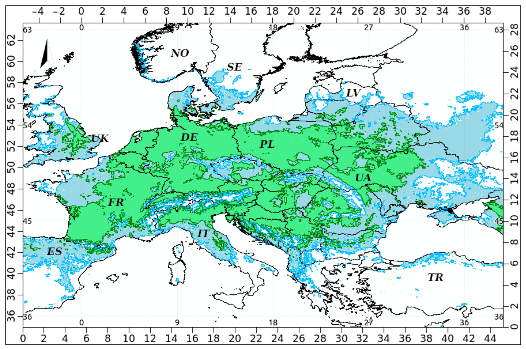
The extent used during the niche modeling process has a profound influence on the outcome of the model [35]. In other words, if the extent under consideration is too limited to represent accessible to the species area via dispersal, the importance of coarse-resolution factors such as climate in delimiting species’ distributions may be underestimated [48]. To represent this area, in SAGA GIS [49] a bounding box was drawn around European point records of the leafminer and buffered to accommodate areas where the black locust is found in Europe. In this way, areas accessible to the species could stretch from Spain and Britain in the west and portions of Nordic countries, to the Caucuses–Caspian region in the east and south to the Mediterranean area and Turkey. Subsequently, environmental raster layers were clipped to this extent.
Climate variables often show high collinearity, and most SDM approaches require the selection of one among strongly correlated variables [50]. In order to carry out such selection, the “removeCollinearity” function in the “virtualspecies” R package was employed [51]. This function analyses the correlation among variables of the provided stack of environmental variables and returns a vector containing names of variables that are not collinear, and also groups variables according to their degrees of collinearity. As climate variables are commonly skewed or have outliers (e.g., when working with precipitation variables), the Spearman correlation method has been used.
SDMs were generated by employing Bayesian additive regression trees (BART), a powerful machine learning approach. Running SDMs with BARTs has recently been substantially facilitated by the development of an R package, “embarcadero” [52], which is highly effective at identifying informative subsets of predictors. Additionally, the package includes methods for generating and plotting partial dependence curves, illustrating the effects of selected variables on habitat suitability. The algorithm computes habitat suitability values ranging from 0, for fully non-suitable habitat, to 1, for fully suitable habitat.
Model performance was assessed using a measure based on the threshold-independent receiver operating characteristic (ROC) approach, where the calculated area under the ROC curve (AUC) is considered as a measure of prediction success [53]. The ROC curve is a graphical method that represents the relationship between the false-positive fraction (one minus the specificity) and the sensitivity for a range of thresholds. It has a range of 0–1: a value greater than 0.5 indicates a better-than-random performance event. A rough classification guide is the traditional academic point system: poor (0.5–0.6), fair (0.6–0.7), good (0.7–0.8), very good (0.8–0.9), and excellent (0.9–1.0).
Maps of habitat suitability in the GeoTIFF format were processed and visualized in SAGA GIS.
Against the background of the appearance of P. robiniella in Kyiv, positive dynamics of the average annual temperature in the city were hypothesized to act as one of the possible factors promoting the invasion of this species; data from the E-OBS (European Observations) website [54] were used for this purpose. Time series data were processed in R [55,56].

3. Results

In total, 1041 records of P. robiniella were collected from European localities. The GBIF database gave above 137,000 records for R. pseudacacia in Europe. For computational reasons, this number of records was reduced to 2447 using the “point thinning” module in SAGA GIS.
Figure 2, Figure 3 and Figure 4 show groups of variables from the three considered databases of environmental predictors according to their degrees of collinearity; names of selected variables that are not collinear are presented in the captions, together with those that have been discarded (Figure 2, Figure 3 and Figure 4).
Ecological niche models are sensitive to sample bias and spatial autocorrelation, which would produce models of lower rather than higher quality [57]; therefore, initial sets or records, for both the moth and black locust, were filtered out using the corresponding module in the “embarcadero” package. Due to the grid resolution issue, the total numbers of records for the moth and tree species were reduced to 832 and 2444, respectively, when predictors were used from the WorldClim v.2 and ENVIREM datasets, and to corresponding 318 and 1940 records, when employing the CliMond v.1.2 set of predictors. In all cases, Moran’s I is <0.3 (p < 0.05).
In Table 1, measures of accuracy are shown for each of the built SDMs: for the moth and host tree using bioclimatic predictors alone; and the other also incorporated the habitat suitability raster for the black locust, assumed to account for biotic interactions.
One of the most crucial in SDM operations is identifying the key environmental variables that determine the niche of the species in question. Usually, SDMs are calibrated only with abiotic variables as predictors, assuming that biotic interactions are indirectly represented by abiotic variables because they strongly correlate [58]. For instance, the presence of the host plant (stonecrop, Sedum L. species) for the caterpillars of the butterfly Parnassius apollo Linnaeus, 1758 is critical; separate SDMs built just upon the use of bioclimatic parameters for the phytophage and host plant strongly correlate (R2 = 0.725, p < 0.05), meaning much of the biotic interaction has been captured [59]. Commonly, it is understood that the addition of biotic interactions usually improves the predictive performance of SDMs [60].
Despite the presumption that climatic factors typically used to represent habitat conditions are rarely adequate surrogates for factors such as host availability [30,61], the AUC measure of accuracy showed that in all three cases, each of the two SDMs built for the moth (one using the corresponding bioclimatic predictors alone, and the other also incorporated the habitat suitability raster for the black locust) performed excellently (AUC values ranging from 0.935 to 0.944, and from 0.926 to 0.943, respectively). Differences between the corresponding AUC values are statistically insignificant (p > 0.05). Additionally, both models in all three cases are highly correlated (p < 0.05): R2 = 96.18%, using the WorldClim v.2 predictors, R2 = 94.21%, using the CliMond v1.2 set, and R2 = 94.06%, using the ENVIREM set of variables.
The variable selection procedure in R package “embarcadero” identified informative subsets of variables, explaining in sum > 60% of variance in the corresponding SDMs (Table 2).
Of these seven predictors ranked in order of their importance, host habitat suitability is represented in each case (Table 2). Perhaps most sharply, this relationship is exemplified in the ENVIREM case, where habitat suitability for the moth rapidly increases with rising habitat suitability for the host tree (Figure 5A). In other words, “better for the host-better for the pest”—said, of course, in terms of the bioclimate. Most likely, the cause of the poorer performance of the SDM being obtained for the black locust itself was that other features essential for the tree (for example, soil) were not considered in the modelling, as the emphasis in this study was on the bioclimate. Nonetheless, at least in terms of the AUC, the SDM performed acceptably (0.740), and showed strong dependence on temperature variables, such as the annual temperature range and the minimum temperature of the coldest month. Similarly, strong dependence on temperature variables has been shown for the black locust in another study employing a maximum entropy model [62].
Interestingly, cold season conditions turned out to be less influential for establishing the moth niche. Such parameters as the maximum temperature of the coldest month (ENVIREM set) and precipitation of driest month (WorldClim v.2 set) have been selected by the BART algorithm; however, they are low ranking in terms of variable importance. Probably, this is because the moths successfully pass the winter at the pupal stage under the reliable protection of leaf litter [19,27].

4. Discussion

Plots of partial dependence curves of identified informative bioclimatic predictors manifesting the model for P. robiniella are presented in Figure 5B and Figure 6A. In Figure 5B, the curve demonstrates the dependence of the well-being of the moth on annual mean temperature (exemplified by the CliMond v.1.2 set). From below the level of 5%, habitat suitability reaches a maximum (approximately 30%) at around an annual mean temperature of 10 °C, and further gradually drops to a more or less stabilized level close to 15% (Figure 5B). Figure 6 represents the response curve for the Thornthwaite aridity index (from the ENVIREM set), based on the relationship between precipitation and potential evapotranspiration, and describes the interplay among rainfall, temperature, and evaporation [63]. On a global scale, the index has been used to categorize the world into nine moisture zones ranging from arid to perhumid [64,65]. From the graph, it can be seen that the highest habitat suitability values for the moth are in the range of 0 < ITh < 20, which relate to a moist subhumid climate (type C2) (Figure 6A).
For building a summarizing model of the potential distribution of P. robiniella in Europe under the current climate, we employed variables explaining in sum > 60% of variance in each of the SDMs built for a separate environmental dataset (Table 2). These are raster images representing black locust habitat suitability, annual mean temperature, annual temperature range, temperature seasonality, growing degree days with mean temperature greater than 0 °C, Thornthwaite aridity index (ITh), and annual precipitation.
Using the SDM and the 10th percentile threshold [65], locations can be found in Europe that are assumed under current climatic conditions to support the spread and naturalization of the moth. In Figure 7, these areas are colored in green and cover a vast range in Western and Central Europe, much of Italy, and the Balkans, reaching as far as the eastern Black Sea region and the Caucasus (Figure 7 and Figure 8). In Ukraine, which is particularly favorable for the pest, there are areas in the west and south-west of the country, and Transcarpathia, bordering the Pannonian Plain. Favorable areas for the moth are predicted in the United Kingdom; however, there have been no records of the moth. As P. robiniella is obviously expanding its home range and is not yet in equilibrium with its environment, we used the 1st percentile threshold as a less conservative threshold to discern between suitable and unsuitable environments. Perhaps in the near future, these areas (colored in blue in Figure 7) will be more widely invaded by the moth, reaching locations in Nordic countries and Estonia, the British Isles, Black Sea coastal areas in Turkey, more of Russia, etc. (Figure 7).
For linking the appearance of P. robiniella in Kyiv with climatic dynamics, average annual temperature records in the city for 1950–2017 were downloaded from the E-OBS database. According to the E-OBS, the average annual temperature in Milano in the 1970s, where P. robiniella was first detected, was 12.99 °C, which assumes that local conditions were favorable for its naturalization, which in fact happened. At that time, the average annual temperature in Kyiv was 8.73 °C, and the difference from Milano was then 4.26 °C. Since 1988, there has been a significant (p < 0.05, 1000 bootstrap) trend of increasing average annual temperature in Kyiv (Figure 6B), and now the difference in temperature between itself and Milano is 64% less than what it was in the 1970s: precisely 2.73 °C. In the 2000s, when P. robiniella was already detected in Kyiv, the average annual temperature was increasingly favorable for the species, −9.70 °C, and in the past decade it has risen to 10.26 °C. In light of our modelling exercises, we consider steeply rising average annual temperatures (perhaps more exactly, temperatures rising on average in the summer, when the moths are active in their development) are involved in setting the scene for the spread and naturalization of the pest, although in a recent study [66] a negative correlation was found between temperature and spread.

5. Conclusions

SDMs seeking to identify features that characterize a species’ known distribution are likely to provide basic quantitative information about the species’ apparent habitat preferences [67,68] and potential distribution. In our study, the extraction of such information was accomplished by the use of the SDM response curves for a number of environmental covariates identified as an informative subset of predictors. Emphasis was put on warmth conditions facilitating the spread and naturalization of the considered pest.
Contrary to the common understanding that the addition of biotic interactions usually improves the predictive performance of SDMs, in our study both sets of SDMs built for P. robiniella (with and without the habitat suitability raster for the host tree) performed equally well.

Author Contributions

Conceptualization, O.N., M.P. and V.T.; data curation, O.N., M.P., A.Č., A.S. and I.K.; formal analysis, O.N., V.T. and O.M.; funding acquisition, M.P. and A.S.; investigation, O.N., M.P., O.M. and I.K.; methodology, O.N. and V.T.; project administration, A.S., A.Č., O.N. and M.P.; resources, O.N. and M.P.; software, O.N. and V.T.; supervision, O.N., V.T. and M.P.; validation, O.N., V.T. and M.P.; Visualization, O.N., V.T. and M.P.; writing—original draft and writing—review and editing, O.N., V.T., M.P., O.M., A.S., A.Č. and I.K. All authors have read and agreed to the published version of the manuscript.

Funding

This study was partly supported by the project “Ecological and socioeconomic thresholds as a basis for defining adaptive management triggers in Latvian pond aquaculture” (lzp-2021/1-0247) and the project “Modern risks of degradation of ecosystems of Ukraine on the example of model zoocenoses: analysis of factors in terms of biological safety” (project #0122U000708).

Institutional Review Board Statement

Not applicable.

Informed Consent Statement

Not applicable.

Data Availability Statement

The data presented in this study are openly available in [Parectopa robiniella. GBIF.org. GBIF Occurrence Download. Available online: https://0-doi-org.brum.beds.ac.uk/10.15468/dl.dp8wtr (accessed on 19 October 2020) and Robinia pseudoacacia. GBIF.org. GBIF Occurrence Download. Available online: https://0-doi-org.brum.beds.ac.uk/10.15468/dl.8f4mb4 (accessed on 5 February 2022)].

Acknowledgments

We are thankful for the help with the project “The mobile complex of Daugavpils University pond aquaculture scientific laboratories” (#16-00-F02201-000002) in the form of providing the mobile complex of scientific laboratories for our research purposes.

Conflicts of Interest

The authors declare no conflict of interest. The funders had no role in the design of the study; in the collection, analyses, or interpretation of data; in the writing of the manuscript, or in the decision to publish the results.

References

  1. State of the Climate Report. 2021. Available online: https://www.ncdc.noaa.gov/sotc/ (accessed on 31 January 2022).
  2. Parmesan, C. Ecological and evolutionary responses to recent climate change. Annu. Rev. Ecol. Evol. Syst. 2006, 37, 637–669. [Google Scholar] [CrossRef] [Green Version]
  3. Root, T.L.; Price, J.T.; Hal, K.R.; Schneider, S.H.; Rosenzweig, C.; Pounds, J.A. Fingerprints of global warming on wild animals and plants. Nature 2003, 421, 57–60. [Google Scholar] [CrossRef] [PubMed]
  4. Nekrasova, O.; Tytar, V.; Pupins, M.; Čeirāns, A.; Marushchak, O.; Skute, A. A GIS Modeling Study of the Distribution of Viviparous Invasive Alien Fish Species in Eastern Europe in Terms of Global Climate Change, as Exemplified by Poecilia reticulata Peters, 1859 and Gambusia holbrooki Girarg, 1859. Diversity 2021, 13, 385. [Google Scholar] [CrossRef]
  5. Nekrasova, O.; Marushchak, O.; Pupins, M.; Skute, A.; Tytar, V.; Čeirāns, A. Distribution and Potential Limiting Factors of the European Pond Turtle (Emys orbicularis) in Eastern Europe. Diversity 2021, 13, 280. [Google Scholar] [CrossRef]
  6. Jepsen, J.U.; Hagen, S.B.; Ims, R.A.; Yoccoz, N.G. Climate change and outbreaks of the geometrids Operophtera brumata and Epirrita autumnata in subarctic birch forest: Evidence of a recent outbreak range expansion. J. Anim. Ecol. 2008, 77, 257–264. [Google Scholar] [CrossRef]
  7. Vidano, C. Foglioline di Robinia pseudoacacia con mine di un microlepidopttero nuotore per l’Italia. L’Apicoltore Mod. 1970, 61, 1–11. [Google Scholar]
  8. Csóka, G.; Pénzes, Z.; Hirka, A.; Mikó, I.; Matošević, D. Parasitoid assemblages of two invading black locust leaf miners, Phyllonorycter robiniella and Parectopa robiniella in Hungary. Period. Biol. 2009, 111, 405–411. [Google Scholar]
  9. EPPO. EPPO Global Database. In EPPO Global Database; EPPO: Paris, France, 2021; Available online: https://gd.eppo.int/ (accessed on 31 January 2022).
  10. Gninenko, Y.I.; Kostukov, V.V.; Kosheleva, O.V. New invasive insects in the forests and greenery of the Krasnodar krai. Zashchita Karantin Rasteniĭ 2011, 4, 49–50. Available online: https://cyberleninka.ru/article/n/novye-invazivnye-nasekomye-v-lesah-i-ozelenitelnyh-posadkah-krasnodarskogo-kraya (accessed on 26 July 2022). (In Russian).
  11. Hrubík, P. Alien insect pests on introduced woody plants in Slovakia. Acta Entomol. Serbica 2007, 12, 81–85. [Google Scholar]
  12. Kollár, J. The harmful entomofauna of woody plants in Slovakia. Acta Entomol. Serbica 2007, 12, 67–79. [Google Scholar]
  13. Ivinskis, P.; Rimšaitė, J. Records of Phyllonorycter robiniella (Clemens, 1859) and Parectopa robiniella Clemens, 1863 (Lepidoptera, Gracillariidae) in Lithuania. Acta Zool. Litu. 2008, 8, 130–133. [Google Scholar] [CrossRef]
  14. Melika, G. Two invading black locust leaf miners, Parectopa robiniella and Phyllonorycter robiniella and their native parasitoid assemblages in Hungary. Biotic damage in forests. In Proceedings of the IUFRO (WP 7.03.10) Symposium, Mátrafüred, Hungary, 12–16 September 2004. [Google Scholar]
  15. Baugnée, J.-Y. Parectopa robiniella (Lepidoptera: Gracillariidae), a leafminer of black locust Robinia pseudoacacia new to the Belgian fauna. Phegea 2014, 42, 55–57. [Google Scholar]
  16. Holoborodko, K.K.; Rusynov, V.I.; Seliutina, O.V. Addition to analysis of morphological parameters of mines on two invasive leaf-mining Lepidoptera species (Parectopa robiniella Clemens, 1863 and Phyllonorycter robiniella Clemens, 1859) on black locust. Issues of bioindication and ecology 2018, 23, 134–141. [Google Scholar] [CrossRef]
  17. Revilla, T.; Gastón, F.J. Nuevas aportaciones a la fauna de Microlepidoptera de España y otras citas de interés (Insecta: Lepidoptera). SHILAP Rev. Lepidopterol. 2019, 47, 57–64. [Google Scholar]
  18. Matsiakh, I.; Kramarets, V. Invasive phyllophagous insects in Ukraine. Sci. Proc. For. Acad. Sci. Ukr. 2020, 20, 11–25. (In Ukrainian) [Google Scholar] [CrossRef]
  19. Shvydenko, I.M.; Stankevych, S.V.; Goroshko, V.V.; Bulat, A.G.; Cherkis, T.M.; Zabrodina, I.V.; Lezhenina, I.P.; Baidyk, H.V. Adventitious leafminer Parectopa robiniella Clemens, 1863 and Phyllonorycter robiniella Clemens, 1859 on a black locust tree in the Kharkiv region. Ukr. J. Ecol. 2021, 11, 22–32. [Google Scholar]
  20. Sautkin, F.V. Arthropod phytophages—Pests of Robinia (Robinia S. L.) in the conditions of Belarus. In Forestry, Nature Management and Processing. Renewable Resources.; Issue 1, BSTU: Minsk, Belarus, 2021; pp. 138–148. [Google Scholar] [CrossRef]
  21. Aarvik, L.; Bengt, A.; Hallvard, E.; Ivinskis, P.; Karsholt, O.; Mutanen, M.; Savenkov, N. Additions and corrections to the Nordic-Baltic Checklist of Lepidoptera. Nor. J. Entomol. 2021, 68, 1–14. [Google Scholar]
  22. Neţoiu, C.; Tomescu, R. Moliile miniere ale salcâmului (Parectopa robiniella Clemens, 1863 şi Phyllonorycter robiniella Clemens, 1859, Lepidoptera, Gracillariidae). An. ICAS 2006, 49, 119–131. [Google Scholar]
  23. Csiha, I.; Keserű, Z.; Rásó, J.; Rédei, K. Black locust (Robinia pseudoacacia L.) selection programmes in Hungary: A short review. Int. J. Hortic. Sci. 2016, 22, 31–34. [Google Scholar] [CrossRef] [Green Version]
  24. Rice, S.K.; Westerman, B.; Federici, R. Impacts of the exotic, nitrogen-fixing black locust (Robinia pseudoacacia) on nitrogen-cycling in a pine-oak ecosystem. Plant Ecol. 2004, 174, 97–107. [Google Scholar] [CrossRef]
  25. Rédei, K.; Keserű, Z.; Csiha, I.; Rásó, J.; Bakti, B.; Takács, M. Improvement of black locust (Robinia pseudoacacia L.) growing under marginal site conditions in Hungary: Case studies. Acta Agrar. Debr. 2018, 74, 129–133. [Google Scholar] [CrossRef]
  26. Stashenko, V.; Politshuk, V. Characteristics of black locust (Robinia pseudoacacia) as a honey plant in the middle Dnepr Region (Ukraine). Am. Bee J. 1998, 138, 665–668. [Google Scholar]
  27. Gninenko, Y.I.; Rakov, A.G. The Locust Digitate Leafminer Parectopa robiniella Cl.—New Invasive Phytophage. Pushkino VNIILM VPRS MOBB 2011, 1–14. Available online: http://www.vniilm.ru/docs/pdf/izdaniya/Edition-Beloakatcievaia-parektopa-robiniella-cl.pdf (accessed on 26 July 2022). (In Russian).
  28. Gubin, A.I.; Martynov, V.V. The first record of the locust digitate leafminer Parectopa robiniella (Clemens, 1863) (Lepidoptera: Gracillariidae) from Georgia. Euroasian Entomol. J. 2017, 16, 304–305. [Google Scholar]
  29. Retevoi, R. Ecological research on the Parectopa robiniella population. Curr. Trends Nat. Sci. 2018, 7, 269–273. [Google Scholar]
  30. Koch, F.H. Considerations regarding species distribution models for forest insects. Agric. For. Entomol. 2021, 23, 393–399. [Google Scholar] [CrossRef]
  31. Parectopa robiniella Clemens. 1863. Available online: https://0-doi-org.brum.beds.ac.uk/10.15468/dl.mqg95f (accessed on 10 June 2022).
  32. Vasyliuk, O.; Prylutskyi, O.; Marushchak, O.; Kuzemko, A.; Kutsokon, I.; Nekrasova, O.; Raes, N.; Rusin, M. An extended dataset of occurrences of species listed in Resolution 6 of the Bern Convention from Ukraine. Biodivers. Data J. 2022, 10, e84002. [Google Scholar] [CrossRef]
  33. Beale, C.M.; Lennon, J.J. Incorporating uncertainty in predictive species distribution modelling. Philos Trans. R. Soc. Lond. B Biol. Sci. 2012, 367, 247–258. [Google Scholar] [CrossRef]
  34. Huntley, J.C. Robinia pseudacacia L. (black locust). In Silvics of North America; Burns, R.M., Honkala, B.H., Eds.; Hardwoods Agricultural Handbook 654: Washington, DC, USA, 1990; Volume 2, pp. 755–761. [Google Scholar] [CrossRef] [Green Version]
  35. Franklin, J. Mapping Species Distributions, Spatial Inference and Prediction; Cambridge University Press: Cambridge, UK, 2009. [Google Scholar] [CrossRef]
  36. Kriticos, D.J. Regional climate-matching to estimate current and future sources of biosecurity threats. Biol. Invasions 2012, 14, 1533–1544. [Google Scholar] [CrossRef]
  37. Venette, R.C. Climate analyses to assess risks from invasive forest insects: Simple matching to advanced models. Curr. For. Rep. 2017, 3, 255–268. [Google Scholar] [CrossRef]
  38. Fick, S.E.; Hijmans, R.J. WorldClim 2: New 1-km spatial resolution climate surfaces for global land areas. Int. J. Climatol. 2017, 37, 4302–4315. [Google Scholar] [CrossRef]
  39. Escobar, L.E.; Lira-Noriega, A.; Medina-Vogel, G.; Peterson, A.T. Potential for spread of the white-nose fungus (Pseudogymnoascus destructans) in the Americas: Use of Maxent and NicheA to assure strict model transference. Geospat. Health 2014, 9, 221–229. [Google Scholar] [CrossRef]
  40. Datta, A.; Schweiger, O.; Kühn, I. Origin of climatic data can determine the transferability of species distribution models. NeoBiota 2020, 59, 61–76. [Google Scholar] [CrossRef]
  41. Kriticos, D.J.; Jarošik, V.; Ota, N. Extending the suite of Bioclim variables: A proposed registry system and case study using principal components analysis. Methods Ecol. Evol. 2014, 5, 956–960. [Google Scholar] [CrossRef]
  42. Title, P.O.; Bemmels, J.B. ENVIREM: An expanded set of bioclimatic and topographic variables increases flexibility and improves performance of ecological niche modeling. Ecography 2018, 41, 291–307. [Google Scholar] [CrossRef] [Green Version]
  43. Tytar, V.M.; Baidashnikov, O. Associations between habitat quality and body size in the Carpathian land snail Vestia turgida: Species distribution model selection and assessment of performance. Zoodiversity 2021, 55, 25–40. [Google Scholar] [CrossRef]
  44. Robinia pseudoacacia L. Available online: https://0-doi-org.brum.beds.ac.uk/10.15468/dl.8f4mb4 (accessed on 5 February 2022).
  45. Nuñez, M.A.; Medley, K.A. Pine invasions: Climate predicts invasion success; something else predictsfailure. Divers. Distrib. 2011, 17, 703–713. [Google Scholar] [CrossRef]
  46. Rangel, T.F.; Diniz-Filho, J.A.F.; Bini, L.M. Towards an integrated computational tool for spatial analysis in macroecology and biogeography. Glob. Ecol. Biogeogr. 2006, 15, 321–327. [Google Scholar] [CrossRef]
  47. Lichstein, J.W.; Simons, T.R.; Shriner, S.A.; Franzreb, K.E. Spatial autocorrelation and autoregressive models in ecology. Ecol. Monogr. 2002, 72, 445–463. [Google Scholar] [CrossRef]
  48. Barve, N.; Barve, V.; Jiménez-Valverde, A.; Lira-Noriega, A.; Maher, S.; Peterson, A.; Soberón, J.; Villalobos, F. The crucial role of the accessible area in ecological niche modeling and species distribution modeling. Ecol. Model. 2011, 222, 1810–1819. [Google Scholar] [CrossRef]
  49. Conrad, O.; Bechtel, B.; Bock, M.; Dietrich, H.; Fischer, E.; Gerlitz, L.; Wehberg, J.; Wichmann, V.; Böhner, J. System for automated geoscientific analyses (SAGA) v. 2.1.4. Geosci. Model Dev. Discuss. 2015, 8, 2271–2312. [Google Scholar] [CrossRef] [Green Version]
  50. Braunisch, V.; Coppes, J.; Arlettaz, R.; Suchant, R.; Schmid, H.; Bollmann, K. Selecting from correlated climate variables: A major source of uncertainty for predicting species distributions under climate change. Ecography 2013, 36, 971–983. [Google Scholar] [CrossRef]
  51. Leroy, B.; Meynard, C.N.; Bellard, C.; Courchamp, F. ‘virtualspecies’: An R package to generate virtual species distributions. Ecography 2016, 39, 599–607. [Google Scholar] [CrossRef]
  52. Carlson, C.J. ‘embarcadero’: Species distribution modelling with Bayesian additive regression trees in R. Methods Ecol. Evol. 2020, 11, 850–858. [Google Scholar] [CrossRef]
  53. Radosavljevic, A.; Anderson, R.P. Making better Maxent models of species distributions: Complexity, overfitting and evaluation. J. Biogeogr. 2014, 41, 629–643. [Google Scholar] [CrossRef]
  54. Moreno, A.; Hasenauer, H. Spatial downscaling of European climate data. Int. J. Climatol. 2016, 36, 1444–1458. [Google Scholar] [CrossRef]
  55. Rumsey, D.J. Statistics for Dummies, 2nd ed.; John Wiley & Sons Inc.: New York, NY, USA, 2016. [Google Scholar]
  56. Mastitskiy, S.E. Analysis of Times Series with R.—Ebook; 2020; Available online: https://ranalytics.github.io/tsa-with-r (accessed on 26 July 2022). (In Russian)
  57. Beck, J.; Ballesteros-Mejia, L.; Nagel, P.; Kitching, I.J. Online solutions and the “Wallacean shortfall”: What does GBIF contribute to our knowledge of species’ ranges? Divers. Distrib. 2013, 19, 1043–1050. [Google Scholar] [CrossRef]
  58. Soberón, J.; Nakamura, M. Niches and distributional areas: Concepts, methods and assumptions. Proc. Natl. Acad. Sci. USA 2009, 106, 19644–19650. [Google Scholar] [CrossRef] [Green Version]
  59. Tytar, V.M. Analysis of home ranges in species: An approach based on modeling the ecological niche. Vestn. Zool. 2011, 25, 96. (In Ukrainian) [Google Scholar]
  60. Araújo, M.B.; Luoto, M. The importance of biotic interactions for modelling species distributions under climate change. Glob. Ecol. Biogeogr. 2007, 16, 743–753. [Google Scholar] [CrossRef]
  61. Lee-Yaw, A.; McCune, J.; Pironon, S.; Sheth, S.N. Species distribution models rarely predict the biology of real populations. Ecography 2022, 2022, e05877. [Google Scholar] [CrossRef]
  62. Li, G.; Xu, G.; Guo, K.; Du, S. Mapping the global potential geographical distribution of Black Locust (Robinia pseudoacacia L.) using herbarium data and a Maximum Entropy Model. Forests 2014, 5, 2773–2792. [Google Scholar] [CrossRef] [Green Version]
  63. Thornthwaite, C.W. An approach toward a rational classification of climate. Geog. Rev. 1948, 38, 55–94. [Google Scholar] [CrossRef]
  64. Feddema, J.J. A revised Thornthwaite-type global climate classification. Phys. Geogr. 2005, 26, 442–466. [Google Scholar] [CrossRef]
  65. Dragot, C.-S.; Popovici, A.; Kucsicsa, G.; Grigorescu, I.; Dumitrascu, S. Land use and crop dynamics related to climate change signals during the post-communist period in the south Oltenia, Romania. Proc. Rom. Acad. Ser. B 2013, 15, 265–278. [Google Scholar]
  66. Mally, R.; Ward, S.F.; Trombik, J.; Buszko, J.; Medzihorsky, V.; Liebhold, A.M. Non-native plant drives the spatial dynamics of its herbivores: The case of black locust (Robinia pseudoacacia) in Europe. NeoBiota 2021, 69, 155–175. [Google Scholar] [CrossRef]
  67. Phillips, S.J.; Dudik, M. Modeling of species distributions with MaxEnt: New extensions and a comprehensive evaluation. Ecography 2008, 31, 161–175. [Google Scholar] [CrossRef]
  68. Nakazato, T.; Warren, D.L.; Moyle, L.C. Ecological and geographic modes of species divergence in wild tomatoes. Am. J. Bot. 2010, 97, 680–693. [Google Scholar] [CrossRef]
Figure 1. Locust digitate leafminer’s (P. robiniella) mines on black locust’s (R. pseudoacacia) leaves, Trukhaniv Island, June 2020.
Diversity 14 00605 g001
Figure 2. Groups of intercorrelated variables from the WorldClim v.2 dataset at cutoff 0.7; the y-axis represents distances between groups (1-Spearman’s r). Variables (var): var1—annual mean temperature, var2—annual precipitation, var4—precipitation driest month, var5—precipitation seasonality, var9—max. temperature of the warmest month, var11—temperature annual range. Discarded variables: var3—precipitation of wettest month, var6—mean diurnal range, var7—isothermality, var8—temperature seasonality, var10—min. temperature of the coldest month.
Diversity 14 00605 g002
Figure 3. Groups of intercorrelated variables from the CliMond v.1.2 dataset at cutoff 0.7; y-axis as in Figure 1. Variables (var): var1—annual mean temperature, var2—mean diurnal temperature range, var4—temperature seasonality, var10—precipitation of driest week, var11—precipitation seasonality, var13—highest weekly radiation, var15 -radiation seasonality, var16—annual mean moisture index, var17—highest weekly moisture index. Discarded variables: var3—isothermality, var5—max. temperature of warmest week, var6—min. temperature of coldest week, var7—temperature annual range, var8—annual precipitation, var9—precipitation of wettest week, var12—annual mean radiation, var14—lowest weekly radiation, var18—lowest weekly moisture index, var19—moisture index seasonality.
Diversity 14 00605 g003
Figure 4. Groups of intercorrelated variables from the ENVIREM dataset to cutoff 0.7; y-axis as in Figure 2. Variables (var): var2—Thornthwaite aridity index (ITh), var4—continentality, var6—growing degree days with mean temperature greater than 0 °C (gdd0), var8—maximum temperature of the coldest month, var13—monthly variability in potential evapotranspiration (PET), var15—mean monthly PET of the warmest quarter, var18—topographic wetness index. Discarded variables: var1—annual PET, var3—climatic moisture index, var5—Emberger’s pluviothermic quotient, var7—growing degree days with mean temperature greater than 5 °C (gdd5), var9—minimum temp. of the warmest month, var10—count of the number of months with mean temp greater than 10 °C, var11—mean monthly PET of coldest quarter, var12—mean monthly PET of driest quarter, var14—mean monthly PET of warmest quarter, var16—thermicity index, var17—terrain roughness index.
Diversity 14 00605 g004
Figure 5. (A) Partial dependence plot for predictor: black locust habitat suitability. Response = predicted moth habitat suitability; blue area = 95% confidence interval; (B) partial dependence plot for predictor: annual mean temperature, °C.
Diversity 14 00605 g005
Figure 6. (A) Partial dependence plot for predictor: Thornthwaite aridity index (ITh); dimensionless. (B) Dynamics of the average annual temperature (AAT) in Kyiv for 1950–2017; x-axis—years, y-axis—AAT (°C); the red dotted line indicates 1988 (‘breakpoint’), after which there is a steady tendency to rising AAT; the arrow marks the time of the first appearance of P. robiniella in Kyiv (2003).
Diversity 14 00605 g006
Figure 7. Map of the potential distribution P. robiniella in Europe. Areas within the 10th percentile threshold are colored in green; areas within the 1st percentile threshold are colored in blue; country codes: France (FR), Germany (DE), Italy (IT), Latvia (LV), Norway (NO), Poland (PL), Spain (ES), Sweden (SE), Turkey (TR), United Kingdom (UK), Ukraine (UA).
Diversity 14 00605 g007
Figure 8. Map of the actual records (non-duplicable) of P. robiniella in Europe [13,14,15,16,17,18,19,20,21,31,32].
Diversity 14 00605 g008
Table 1. Measures of accuracy of produced SDMs. *—SDMs built for P. robiniella (P), R. pseudoacacia (R) and P. robiniella incorporating the habitat suitability raster for R. pseudoacacia (P+R).
WorldClim v.2CliMond v1.2ENVIREM
SDMs *PRP+RPRP+RPRP+R
AUC0.9350.7700.9360.9360.7720.9260.9440.7720.943
±SE0.0090.0100.0090.0120.0110.0120.0090.0100.008
Table 2. Variables explaining in sum > 60% of variance in the SDM (ranked in order of variable importance).
WorldClim v.2CliMond v.1.2ENVIREM
1. Annual mean temperature
2. Host habitat suitability
3. Temperature annual range
4. Annual mean precipitation
1. Temperature seasonality
2. Annual mean temperature
3. Host habitat suitability
1. Host habitat suitability
2. Thornthwaite aridity index (ITh)
3. gdd0
Publisher’s Note: MDPI stays neutral with regard to jurisdictional claims in published maps and institutional affiliations.

