
Robust Decentralized Nonlinear Control for a Twin Rotor MIMO System

 ,
,  and
and
Abstract
:
1. Introduction
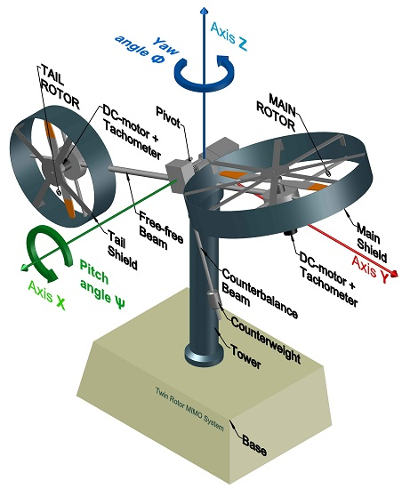
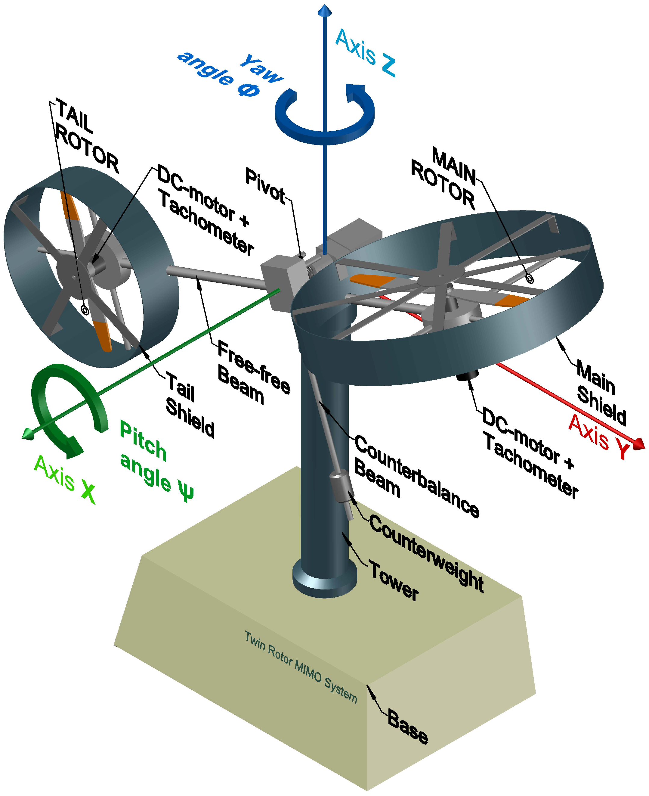
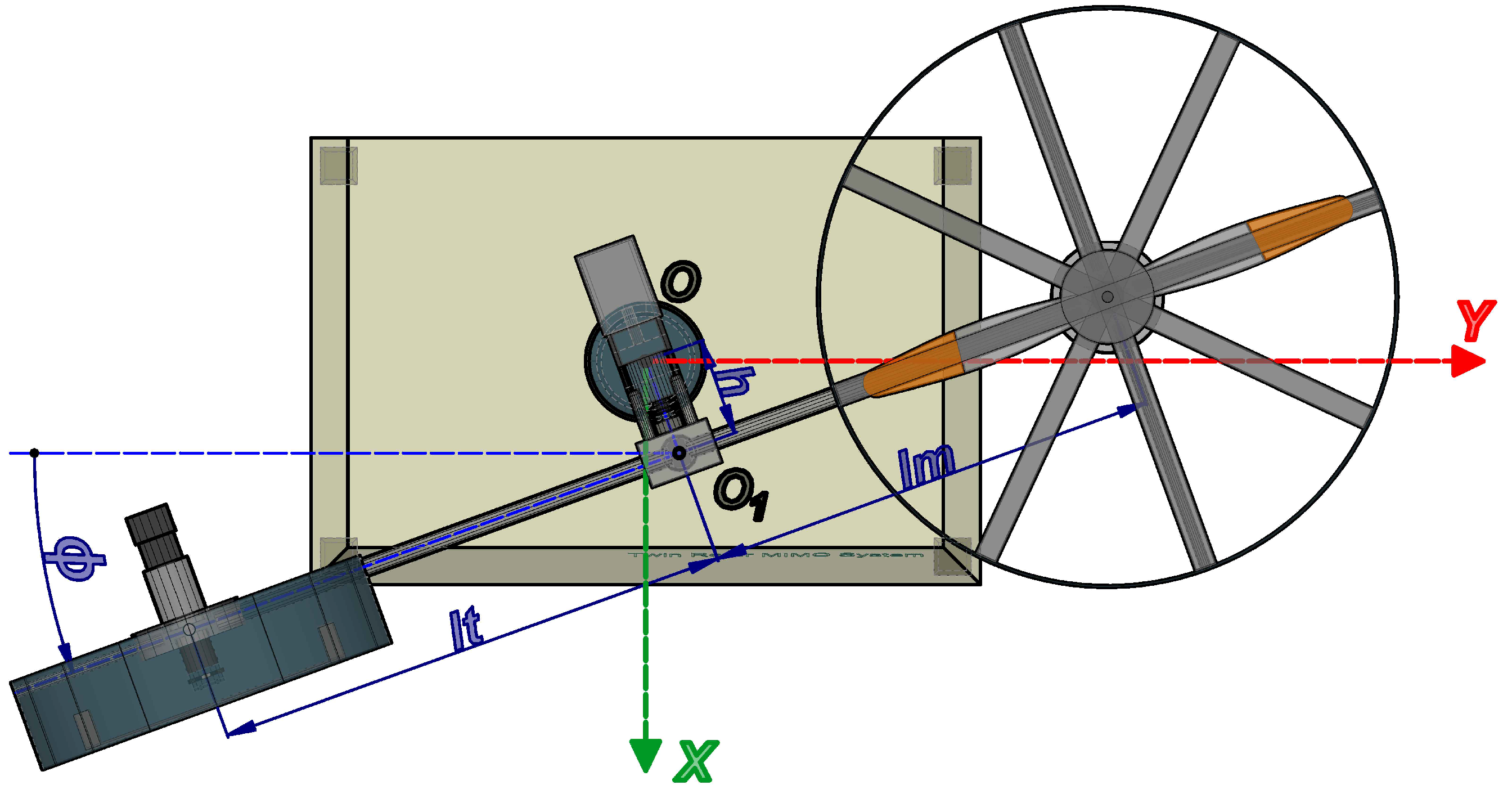
2. Dynamic Model
2.1. Dynamics of the Electrical Part
- Main rotor:
- Tail rotor:
2.2. Dynamics of the Mechanical Part
2.2.1. Evaluation of the Kinetic Energy
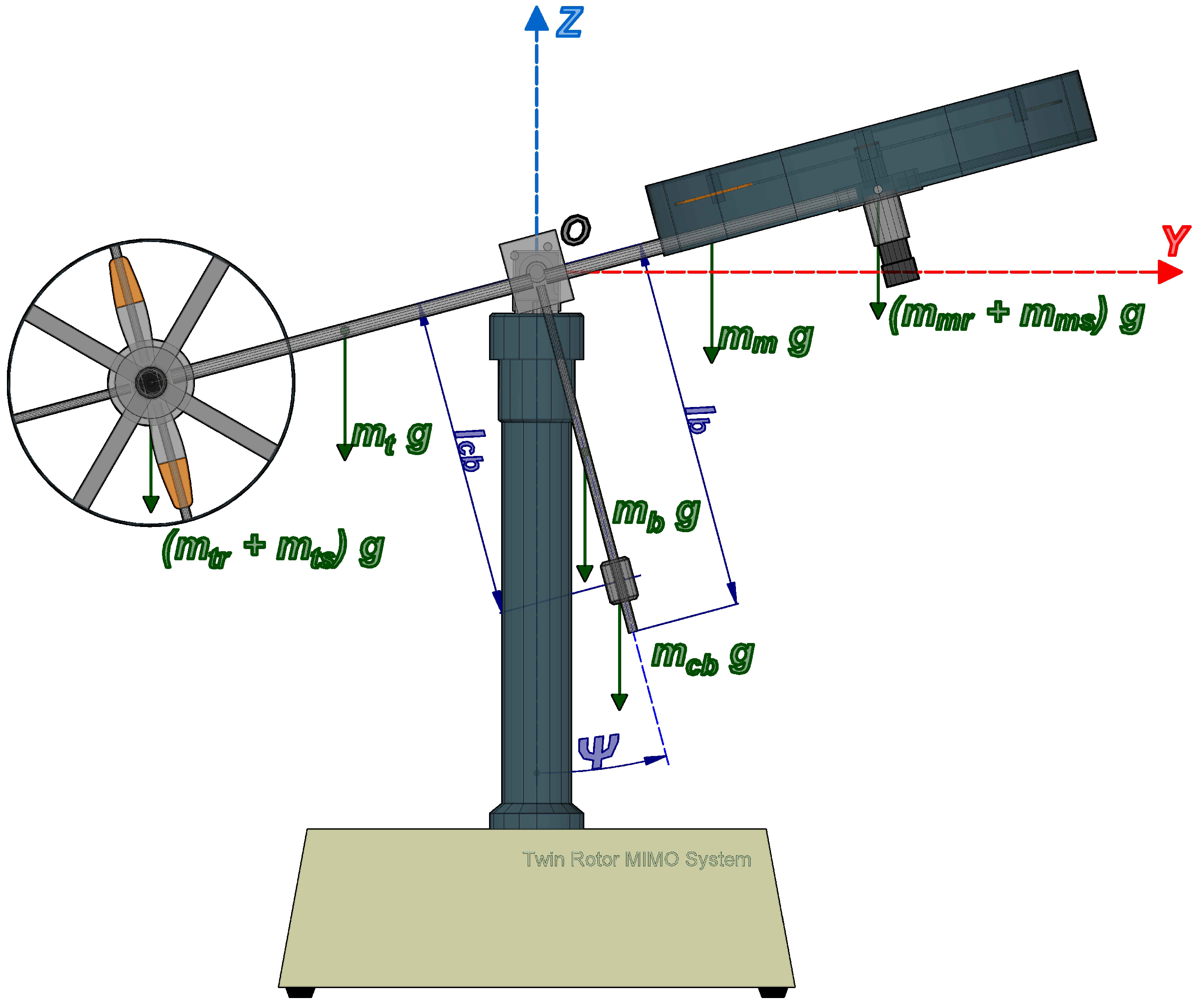
2.2.2. Evaluation of the Potential Energy
2.2.3. Lagrangian
2.2.4. Generalized Forces
2.2.5. Equations of Motion
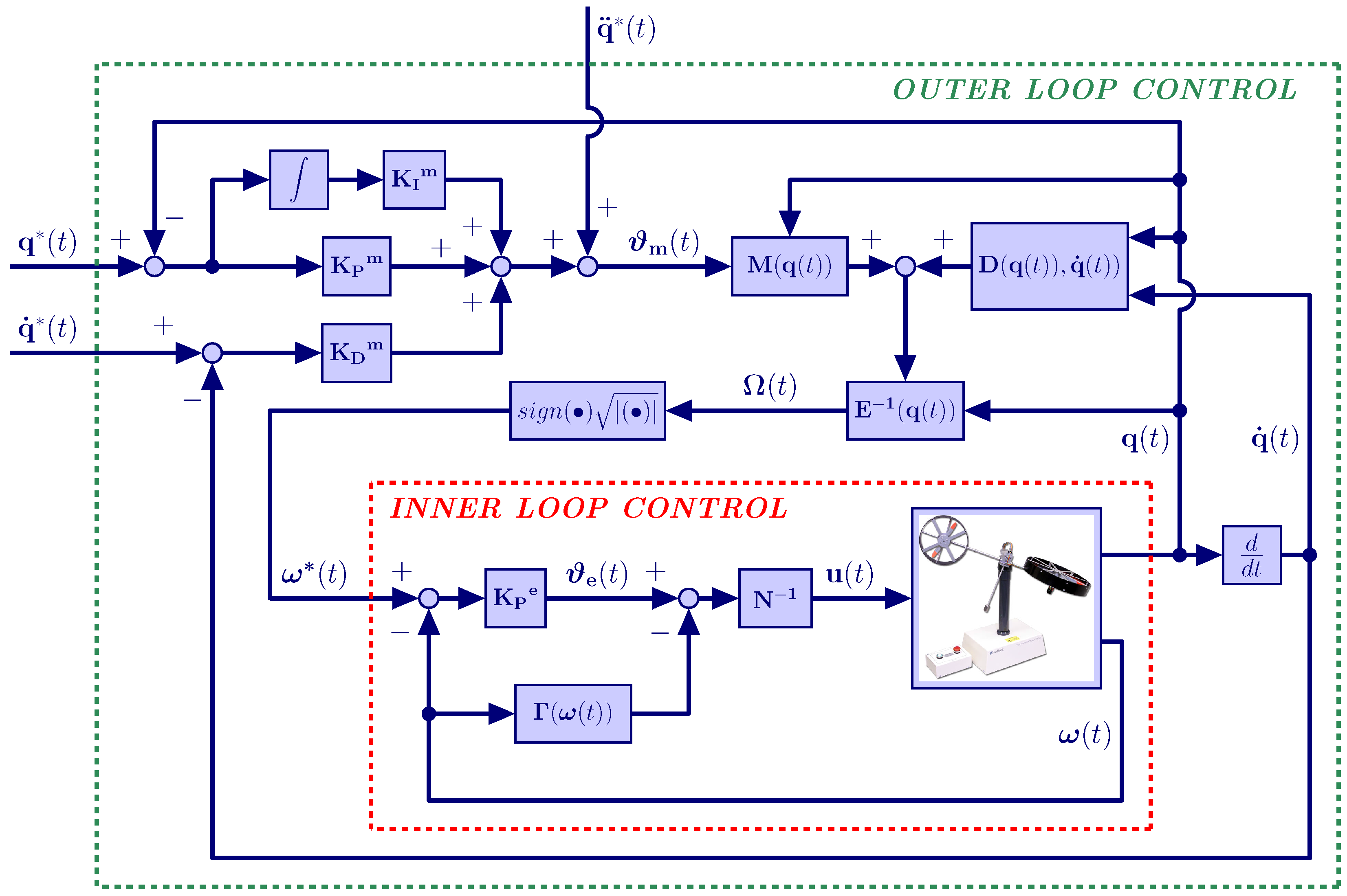
3. Design of the Control System
3.1. Inner Loop Control
3.2. Outer Loop Control
4. Experimental Section
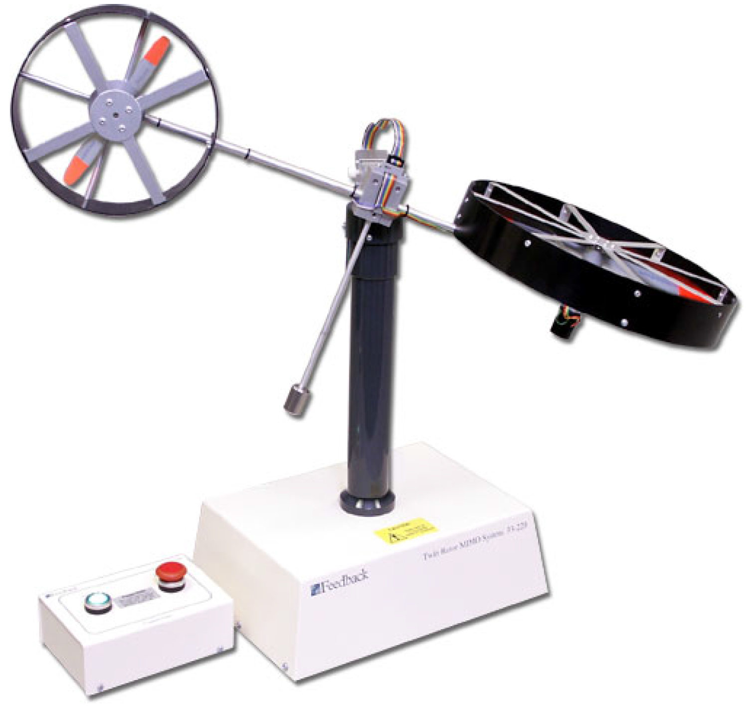
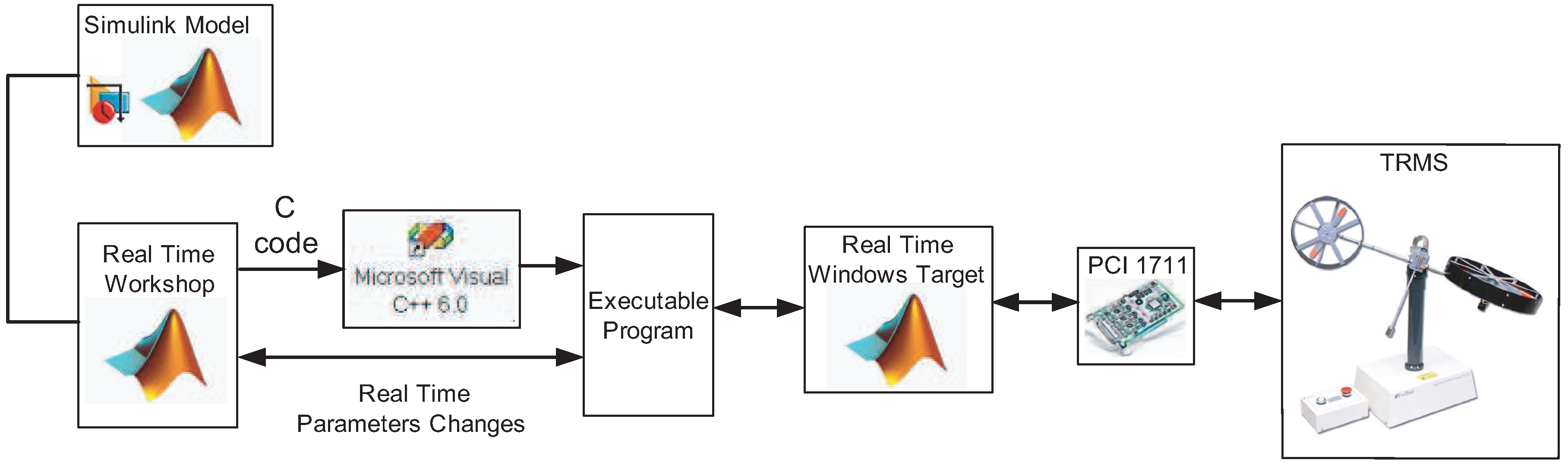
4.1. Experimental Setup
- A PC operating in a Windows® environment using software tools from MathWorks® Inc (MATLAB®, Simulink, Control Toolbox, Real Time Workshop® (RTW), Real Time Windows Target® (RTWT)) and Visual Professional®.
- The real TRMS is connected to the computer by means of an Advantech® PCI1711 card, which is accessible in the MATLAB/Simulink® environment through the Real-Time Toolbox®.
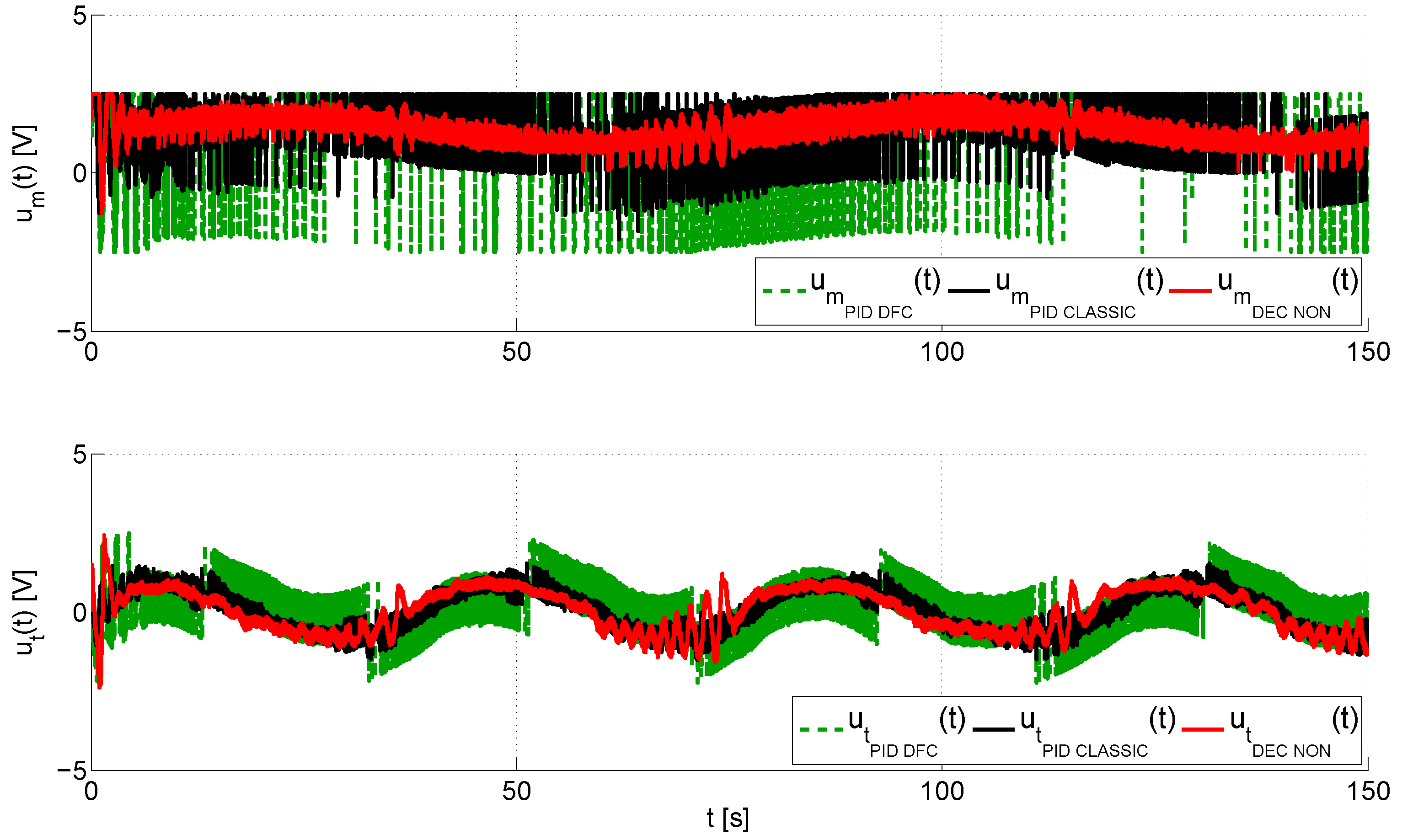
- The control signals in the MATLAB/Simulink® environment consist of two input voltages (in the range V) for the two DC motors A-max 26 provided by Maxon Motor®.
- The vector of generalized coordinates, , are measured by using two HCTL 2016 digital encoders provided by Agilent Technologies®, and the angular velocity vector is measured by using two DC-Tacho DCT 22 provided by Maxon Motor®.
- The sampling rate for the controlled system is s.
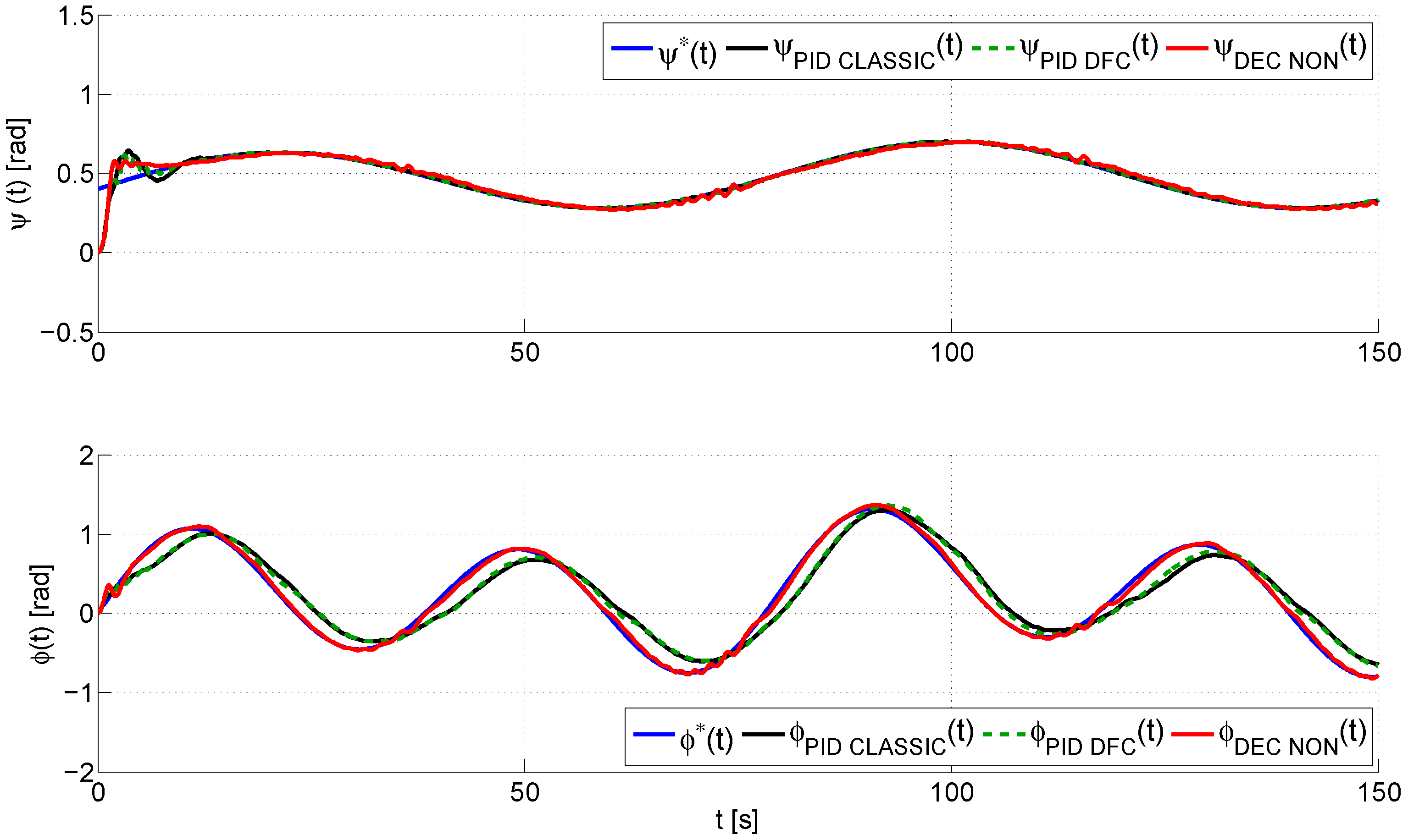
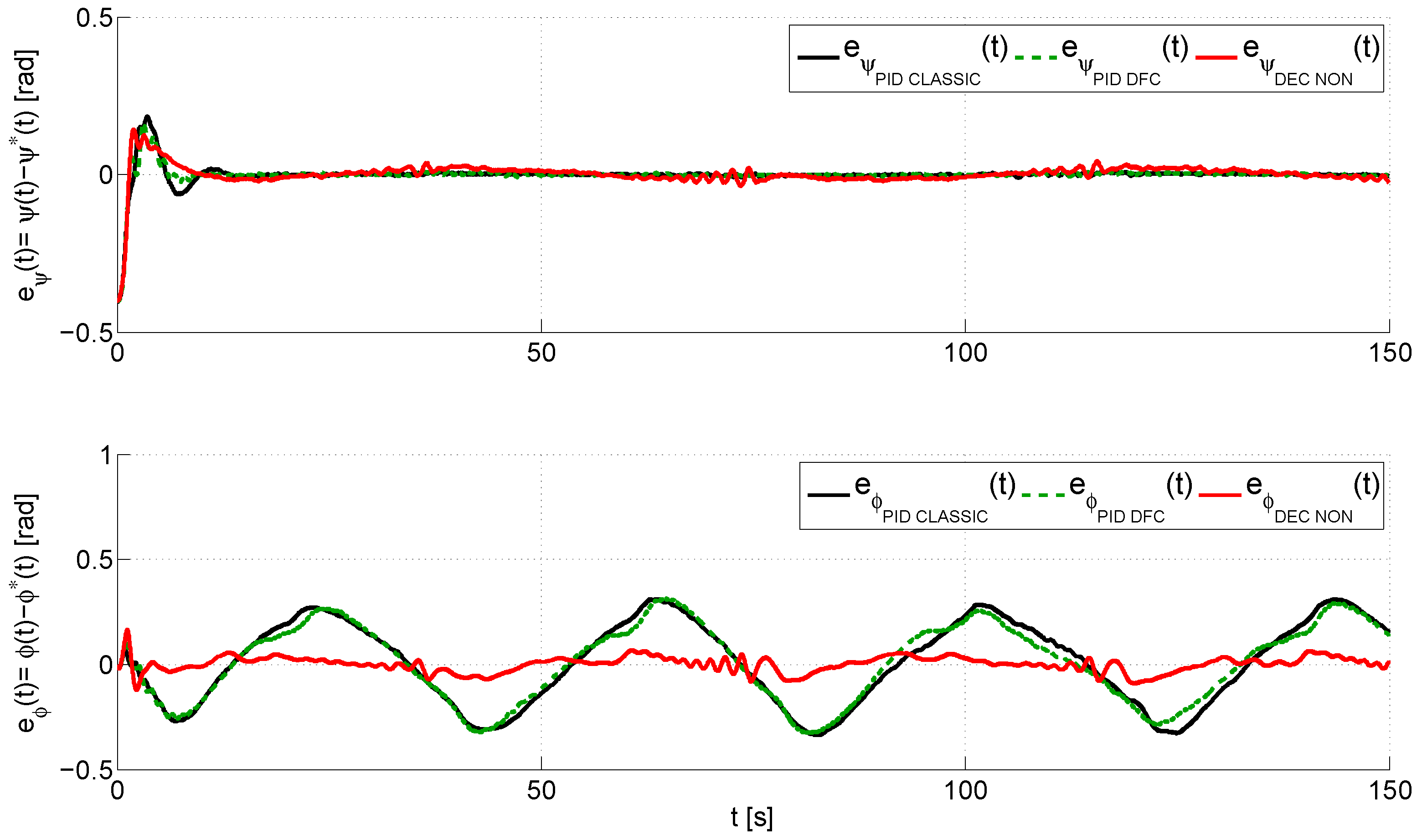
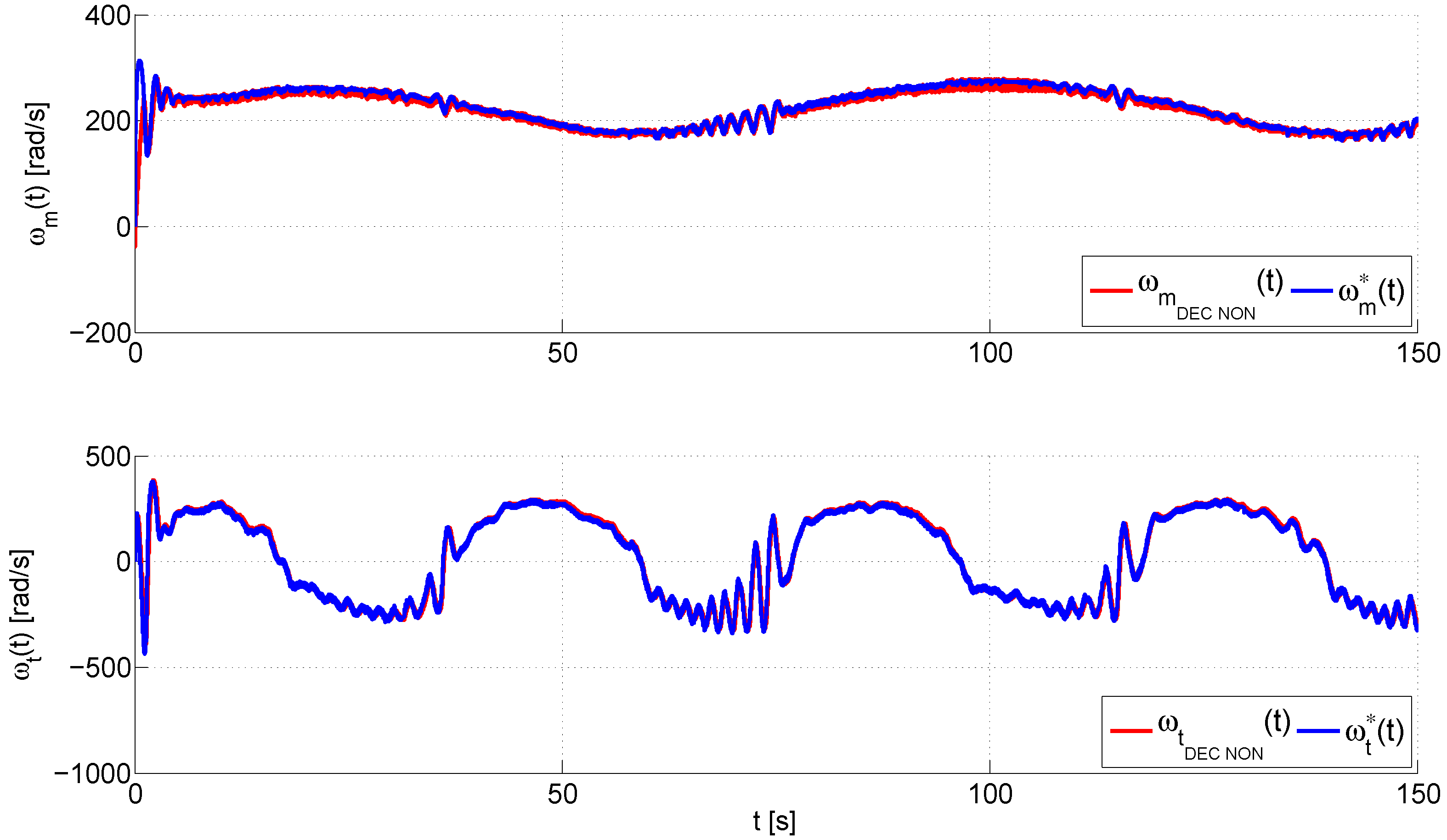
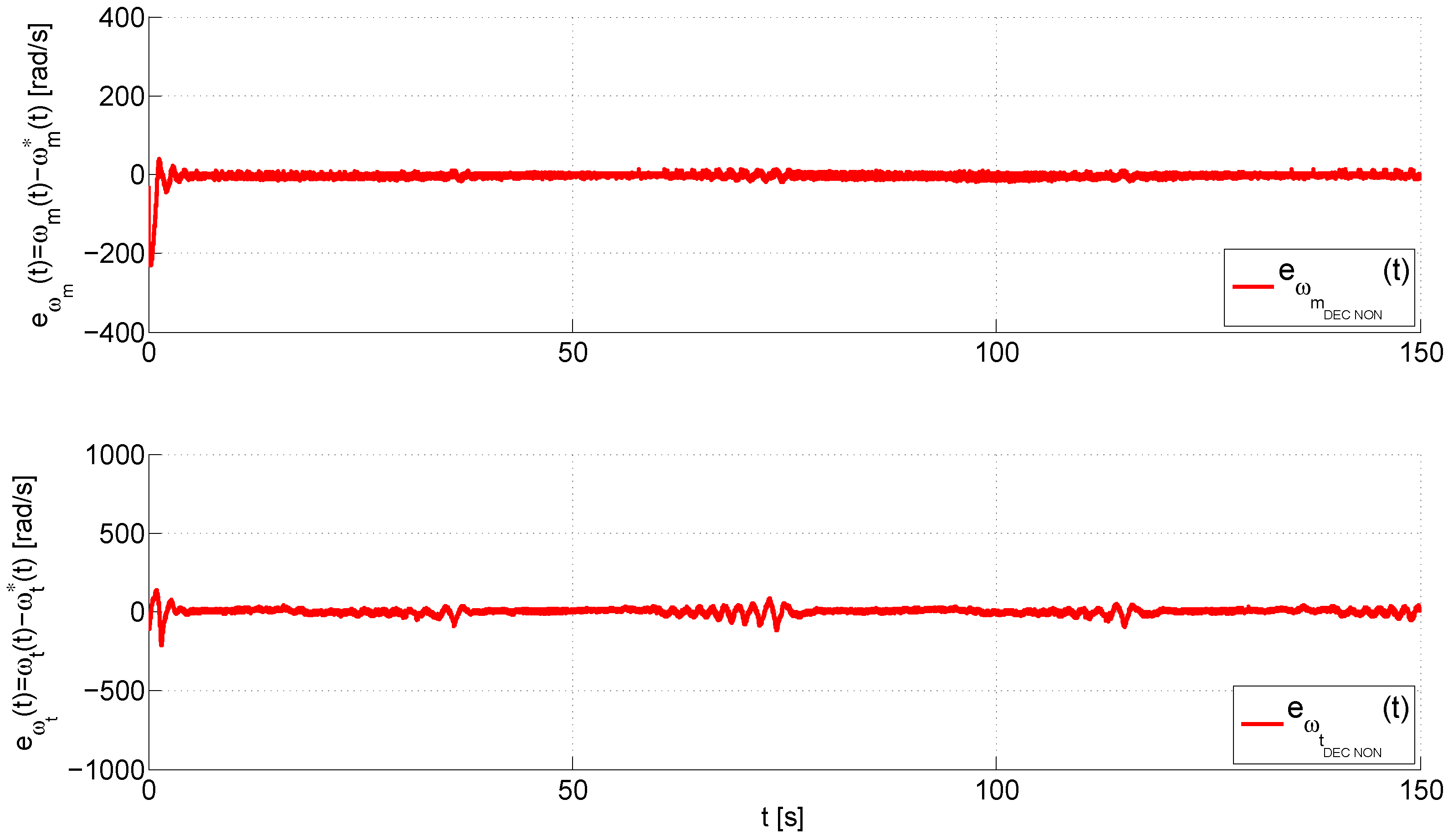
4.2. Experimental Results
5. Conclusions
Acknowledgments
Author Contributions
Conflicts of Interest
References
- Nonami, K.; Kendoul, F.; Suzuki, S.T. Autonomous Flying Robots—Unmanned Aerial Vehicles and Micro Aerial Vehicles; Springer: Heidelberg, Germany, 2010. [Google Scholar]
- Espizona, T.; Dzul, A.; Llama, M. Linear and Nonlinear Controllers Applied to Fixed-Wing UAV. Int. J. Adv. Robot. Syst. 2013, 10, 33. [Google Scholar] [CrossRef]
- Fernández-Caballero, A.; Belmonte, L.M.; Morales, R.; Somolinos, J.A. Generalized Proportional Integral Control for an Unmanned Quadrotor System. Int. J. Adv. Robot. Syst. 2015, 12, 85. [Google Scholar] [CrossRef]
- Alvarenga, J.; Vitzilaios, N.I.; Valavanis, K.P.; Rutherford, M.J. Survey of Unmanned Helicopter Model-Based Navigation and Control Techniques. J. Intell. Robot. Syst. 2015, 80, 87–138. [Google Scholar] [CrossRef]
- Ali, Z.A.; Wang, D.; Aamir, M. Fuzzy-Based Hybrid Control Algorithm for the Stabilization of a Tri-Rotor UAV. Sensors 2016, 16, 652. [Google Scholar] [CrossRef] [PubMed]
- Cabecinhas, D.; Naldi, R.; Silvestre, C.; Cunha, R.; Marconi, L. Robust Landing and Sliding Maneuver Hybrid Controller for a Quadrotor Vehicle. IEEE Trans. Control Syst. Technol. 2016, 4, 400–412. [Google Scholar] [CrossRef]
- Chen, F.; Wu, Q.; Jiang, B.; Tao, G. A Reconfiguration Scheme for Quadrotor Helicopter via Simple Adaptive Control and Quantum Logic. IEEE Trans. Ind. Electron. 2015, 62, 4328–4335. [Google Scholar] [CrossRef]
- Zheng, B.; Zhong, Y. Robust Attitude Regulation of a 3-DOF Helicopter Benchmark: Theory and Experiments. IEEE Trans. Ind. Electron. 2011, 58, 660–670. [Google Scholar] [CrossRef]
- Feedback Co. Twin Rotor MIMO System 33-220 User Manual; Feedback Co.: Crowborough, UK, 1998. [Google Scholar]
- Rahideh, A.; Shaheed, M.H.; Huigberts, H.J.C. Dynamic Modelling of a TRMS Using Analytical and Empirical Approaches. Control Eng. Pract. 2008, 16, 241–259. [Google Scholar] [CrossRef]
- Toha, S.F.; Latiff, I.A.; Mohamad, M.; Tokhi, M.O. Parametric modelling of a TRMS using dynamic spread factor particle swarm optimisation. In Proceedings of the UKSim 2009: 11th International Conference on Computer Modelling and Simulation, Cambridge, UK, 25–27 March 2009; pp. 95–100.
- Tanaka, H.; Ohta, Y.; Okimura, Y. A local approach to LPV-identification of a Twin Rotor MIMO System. IFAC Proc. Vol. 2011, 44, 7749–7754. [Google Scholar] [CrossRef]
- Tastemirov, A.; Lecchini-Visintini, A.; Morales, R.M. Complete Dynamic Model of the TWIN Rotor MIMO System (TRMS) with Experimental Validation. In Proceedings of the 39th European Rotorcraft Forum 2013 (ERF 2013), Moscow, Russia, 3–6 September 2013.
- Chalupa, P.; Prikryl, J.; Novák, J. Modelling of Twin Rotor MIMO System. Procedia Eng. 2015, 100, 249–258. [Google Scholar] [CrossRef]
- Juang, J.-G.; Lin, R.-W.; Liu, W.-K. Comparison of classical control and intelligent control for a MIMO system. Appl. Math. Comput. 2008, 25, 778–791. [Google Scholar] [CrossRef]
- Wen, P.; Lu, T.W. Decoupling control of a twin rotor mimo system using robust deadbeat control technique. IET Control Theory Appl. 2008, 2, 999–1007. [Google Scholar] [CrossRef]
- Rahideh, A.; Shaheed, M.H. Constrained output feedback model predictive control for nonlinear systems. Control Eng. Pract. 2012, 20, 431–443. [Google Scholar] [CrossRef]
- Jahed, M.; Farrokhi, M. Robust adaptive fuzzy control of twin rotor MIMO system. Soft Comput. 2013, 17, 1847–1860. [Google Scholar] [CrossRef]
- Kumar-Pandey, S.; Laxmi, V. Control of Twin Rotor MIMO System using PID controller with derivative filter coefficient. In Proceedings of the 2014 IEEE Students’ Conference on Electrical, Electronics and Computer Science, Bhopal, India, 1–2 March 2014.
- Belmonte, L.M.; Morales, R.; Fernández-Caballero, A.; Somolinos, J.A. A Tandem Active Disturbance Rejection Control for a Laboratory Helicopter with Variable Speed Rotors. IEEE Trans. Ind. Electron. 2016. [Google Scholar] [CrossRef]
- Alagoz, B.B.; Ates, A.; Yeroglu, C. Auto-tuning of PID controller according to fractional-order reference model approximation for DC rotor control. Mechatronics 2013, 23, 789–797. [Google Scholar] [CrossRef]
- Mullhaupt, P.; Srinivasan, B.; Levine, J.; Bonvin, D. Control of the Toycopter Using a Flat Approximation. IEEE Trans. Control Syst. Technol. 2008, 16, 882–896. [Google Scholar] [CrossRef] [Green Version]
- Morales, R.; Feliu, V.; Jaramillo, V. Position control of very lightweight single-link flexible arms with large payload variations by using disturbance observers. Robot. Auton. Syst. 2012, 60, 532–547. [Google Scholar] [CrossRef]
- Son, Y.I.; Kim, I.H.; Choi, D.S.; Shim, D. Robust Cascade Control of Electric Motor Drives Using Dual Reduced-Order PI Observers. IEEE Trans. Ind. Electron. 2015, 62, 3672–3682. [Google Scholar] [CrossRef]
- Marlin, T.E. Process Control, Designing Processes and Control Systems for Dynamic Performance, 2nd ed.; McGraw-Hill: New York, NY, USA, 2000. [Google Scholar]
- Arrieta, O.; Vilanova, R.; Balaguer, P. Procedure for cascade control systems design: Choice of suitable PID tunings. Int. J. Comput. Commun. Control 2008, 3, 235–248. [Google Scholar] [CrossRef]
- Alfaro, V.M.; Vilanova, R.; Arrieta, O. Robust tuning of Two-Degree-of-Freedom (2-DoF) PI/PID based cascade control systems. J. Process Control 2009, 19, 1658–1670. [Google Scholar] [CrossRef]
- Veronesi, M.; Visioli, A. Simultaneous closed-loop automatic tuning method for cascade controllers. IET Control Theory Appl. 2011, 5, 263–270. [Google Scholar] [CrossRef]
- Feedback Co. Twin rotor MIMO system. Control Experiments; Manual 33-949S Ed01; Feedback Co.: Crowborough, UK, 2008. [Google Scholar]


| Symbol | Parameter | Value | Units |
|---|---|---|---|
| Parameters of the Main Rotor | |||
| Motor velocity constant | |||
| Motor armature resistance | 8 | Ω | |
| Motor armature inductance | H | ||
| Electromagnetic constant torque motor | |||
| Coefficient linear relationship interface circuit | − | ||
| Load factor () | |||
| Load factor () | |||
| Viscous friction coefficient | |||
| Moment of inertia about the axis of rotation | |||
| Electrical time constant () | s | ||
| Mechanical time constant () | s | ||
| Parameters of the Tail Rotor | |||
| Motor velocity constant | |||
| Motor armature resistance | 8 | Ω | |
| Motor armature inductance | H | ||
| Electromagnetic constant torque motor | |||
| Coefficient linear relationship interface circuit | − | ||
| Load factor | |||
| Viscous friction coefficient | |||
| Moment of inertia about the axis of rotation | |||
| Electrical time constant () | s | ||
| Mechanical time constant () | s | ||
| Symbol | Parameter | Value | Units |
|---|---|---|---|
| Length of the tail part of the free-free beam | m | ||
| Length of the main part of the free-free beam | m | ||
| Length of the counterbalance beam | m | ||
| Distance between the counterweight and the joint | m | ||
| Radius of the main shield | m | ||
| Radius of the tail shield | m | ||
| h | Length of the pivoted beam | m | |
| Mass of the tail DC motor and tail rotor | kg | ||
| Mass of the main DC motor and main rotor | kg | ||
| Mass of the counterweight | kg | ||
| Mass of the tail part of the free-free beam | kg | ||
| Mass of the main part of the free-free beam | kg | ||
| Mass of the counterbalance beam | kg | ||
| Mass of the tail shield | kg | ||
| Mass of the main shield | kg | ||
| Mass of the pivoted beam | kg |
| Symbol | Parameter | Value | Units |
|---|---|---|---|
| Parameters of the Pitch movement | |||
| Thrust torque coefficient of the main rotor () | |||
| Thrust torque coefficient of the main rotor () | |||
| Load torque coefficient of the tail rotor | |||
| Viscous friction coefficient | |||
| Coulomb friction coefficient | |||
| Coefficient of the inertial counter torque due to change in | |||
| Parameters of the Yaw movement | |||
| Thrust torque coefficient of the tail rotor () | |||
| Thrust torque coefficient of the tail rotor () | |||
| Load torque coefficient of the main rotor () | |||
| Load torque coefficient of the main rotor () | |||
| Viscous friction coefficient | |||
| Coulomb friction coefficient | |||
| Coefficient of the elastic force torque created by the cable | |||
| Constant for the calculation of the torque of the cable | 0 | ||
| Coefficient of the inertial counter torque due to change in | |||
| Control Method | ISE | IAE | ITAE |
|---|---|---|---|
| Robust Decentralized Nonlinear Control (DEC NON) | |||
| Standard PID control (PID CLASSIC) | |||
| PID control with the derivative filter coefficient (PID DFC) |
© 2016 by the authors; licensee MDPI, Basel, Switzerland. This article is an open access article distributed under the terms and conditions of the Creative Commons Attribution (CC-BY) license (http://creativecommons.org/licenses/by/4.0/).
Share and Cite
Belmonte, L.M.; Morales, R.; Fernández-Caballero, A.; Somolinos, J.A. Robust Decentralized Nonlinear Control for a Twin Rotor MIMO System. Sensors 2016, 16, 1160. https://0-doi-org.brum.beds.ac.uk/10.3390/s16081160
Belmonte LM, Morales R, Fernández-Caballero A, Somolinos JA. Robust Decentralized Nonlinear Control for a Twin Rotor MIMO System. Sensors. 2016; 16(8):1160. https://0-doi-org.brum.beds.ac.uk/10.3390/s16081160
Chicago/Turabian StyleBelmonte, Lidia María, Rafael Morales, Antonio Fernández-Caballero, and José Andrés Somolinos. 2016. "Robust Decentralized Nonlinear Control for a Twin Rotor MIMO System" Sensors 16, no. 8: 1160. https://0-doi-org.brum.beds.ac.uk/10.3390/s16081160